Abstract
This paper proposes a method for forecasting surface solar irradiance (SSI), the most critical factor in solar photovoltaic (PV) power generation. The proposed method uses 16-channel data obtained by the GEO-KOMPSAT-2A (GK2A) satellite of South Korea as the main data for SSI forecasting. To determine feature variables related to SSI from the 16-channel data, the differences and ratios between the channels were utilized. Additionally, to consider the fundamental characteristics of SSI originating from the sun, solar geometry parameters, such as solar declination (SD), solar elevation angle (SEA), and extraterrestrial solar radiation (ESR), were used. Deep learning-based feature selection (Deep-FS) was employed to select appropriate feature variables that affect SSI from various feature variables extracted from the 16-channel data. Lastly, spatio-temporal deep learning models, such as convolutional neural network–long short-term memory (CNN-LSTM) and CNN–gated recurrent unit (CNN-GRU), which can simultaneously reflect temporal and spatial characteristics, were used to forecast SSI. Experiments conducted to verify the proposed method against conventional methods confirmed that the proposed method delivers superior SSI forecasting performance.
1. Introduction
1.1. Motivation
Renewable energy is defined as environmentally friendly and clean energy with low CO2 generation. Energy obtained from non-depletable energy sources, such as the sun and wind, can be indefinitely renewable. Therefore, renewable energy as a countermeasure against climate change and its adverse effects, such as energy competition and global warming due to fossil fuel depletion, is becoming increasingly important. Among the various power generation technologies using renewable energy, solar photovoltaic (PV) power generation, which uses solar cells to convert solar energy into electricity, has been growing rapidly in recent years due to its ease of installation and policy supports. Because of advances in solar PV power generation, its energy efficiency has improved, and costs are gradually decreasing. Thus, solar energy is being recognized as a more economical and sustainable option. Consequently, electricity production using solar PV power generation and, thereby, dependence on this avenue of energy production are increasing rapidly worldwide. This global trend of solar PV power generation emphasizes its importance in modern society. In the future, solar PV power generation is expected to become the core of the energy industry. Moreover, research and technological innovation in solar PV power generation have the potential to emerge as highly important endeavors.
1.2. Problem Statement
Solar PV power generation fluctuates depending on weather conditions. This volatility adversely affects the operation stability of the power system. Such instability can cause blackouts and an increase in power prices. Therefore, technology to forecast the amount of solar PV power generation is required to alleviate the aforementioned problems and establish a stable power supply and demand plan. Because solar PV power generation converts solar energy into electrical energy, there is a high correlation between the amount of power generation and solar irradiance. Therefore, elements related to solar irradiance, such as global horizontal irradiance (GHI), diffuse horizontal irradiance (DHI), and direct normal irradiance (DNI), have been used in many studies on forecasting the amount of solar PV power generation [1,2,3,4]. Factors affecting solar irradiance reaching the surface, such as sky condition, clearness index, visibility, cloud cover, and date, have also been investigated [5,6,7]. Furthermore, studies focusing on forecasting the amount of solar PV power generation are preceded by solar irradiance forecasting [8,9]. In this context, it can be inferred that solar irradiance is the most critical factor in forecasting the amount of solar PV power generation. Therefore, research on solar irradiance forecasting needs to be pursued as a precedent.
1.3. Related Works
In the past, research on solar irradiance forecasting was mainly based on statistical methods such as autoregressive moving average (ARMA), autoregressive integrated moving average (ARIMA), and seasonal autoregressive integrated moving average (SARIMA) [10,11,12,13]. Statistical methods work by identifying patterns and trends observed in time series data to make forecasting. However, statistical methods have limitations in that they rely on linear relationships in the data, making it challenging to model non-linear relationships, and they traditionally rely only on historical data, which can limit forecasting. To overcome the limitations mentioned above, recent efforts have been made to utilize traditional machine learning methods such as random forest (RF), support vector regression (SVR), or deep learning methods such as an artificial neural network (ANN), long short-term memory (LSTM), gated recurrent unit (GRU), and convolutional neural network (CNN) [14,15,16,17,18,19,20]. Approaches using machine learning and deep learning can easily model non-linear relationships and flexibly handle a variety of data to provide more accurate forecasting. In particular, deep learning can learn complex patterns and trends, making them adaptable to environmental changes or new data. For this reason, solar irradiance forecasting using machine learning and deep learning has been a growing area of research in recent years.
The following are studies that apply machine learning to solar irradiance forecasting: Urraca et al. [14] used RF and SVR to forecast 1 h–ahead GHI. The authors applied parameter optimization utilizing cross-validation, feature selection based on genetic algorithm (GA), and model optimization using parsimonious model selection to differentiate from conventional methods. Additionally, the authors compared the performance with and without the differentiated methods and selected the best-performing model. They used various performance metrics, such as mean absolute error (MAE), root mean square error (RMSE), mean bias error (MBE), normalized mean absolute error (NMAE), normalized root mean square error (NRMSE), and forecast skill for performance evaluation. They compared performance with a persistence model and found that both SVR and RF outperformed the persistence model, while both models were effectively simplified and reduced the number of features as input variables. Yang et al. [15] conducted a study for easy and efficient hourly global solar radiation prediction. The authors considered three machine-learning models for global solar radiation prediction: back propagation network (BP), SVR, and light gradient boosting machine (LightGBM). Additionally, they utilized various meteorological factors and extra-terrestrial solar radiation (ESR) derived from solar geometry. Then, they used a Shapley additive explanation (SHAP) model to select appropriate factors affecting global solar radiation from the available factors. As a result, they selected seven input variables based on feature importance: ESR, cloud cover, air temperature, relative humidity, date, and hour. They also compared the model’s performance with and without the weather type variable, representing 18 different weather types, and found that the model performed better with the weather-type variable. Finally, they compared the prediction performance of the three machine learning methods and found that LightGBM performed the best.
In the studies on solar irradiance forecasting using machine learning, studies were compared with and without the proposed unique techniques, or the performance was verified by comparing the performance with traditional methods. Since there are many parameters that determine machine learning models compared to statistical models, various methods for model optimization have been proposed, and it is confirmed that efforts have been made to select appropriate variables that influence solar irradiance.
The following are studies that apply deep learning to solar irradiance forecasting: Brahma et al. [16] forecasted daily solar irradiance after 1, 4, and 10 d using multi-regional data and a deep learning model specialized for time-series data forecasting. They used LSTM, GRU, CNN, bi-directional LSTM (Bi-LSTM), and attraction LSTM to forecast solar irradiance and employed Pearson correlation, Spearman correlation, and extreme gradient boosting to select surrounding areas that are highly related to solar irradiance in the target area. They also used autocorrelation to determine the appropriate number of days of historical data and rolling window evaluation to assess the model in terms of accuracy, robustness, and reliability. Meanwhile, Huang et al. [17] forecasted solar irradiance after 1 h using a hybrid deep learning model combining wavelet packet decomposition (WPD) and various deep learning models. They subsequently compared and analyzed the forecasting performance of different combinations of hybrid deep learning models. Consequently, they concluded that the highest solar irradiance forecasting performance is obtained using WPD-CNN-LSTM-MLP, which combines WPD, CNN, LSTM, and multi-layer perceptron (MLP). Their input variables in training their model included temperature, relative humidity, wind speed, and solar irradiance over the last 24 h. Meanwhile, Rajagukguk et al. [18] forecasted solar irradiance using sky images captured through a sky camera. First, they used the red–blue ratio method and Otsu threshold to derive cloud cover, which affects solar irradiance, from the sky images. Then, they employed LSTM to forecast cloud cover and used a physical model based on forecasted cloud cover to forecast solar irradiance. Nielsen et al. [19] forecasted effective cloud albedo (CAL) based on convolutional–LSTM (ConvLSTM) using satellite data to forecast solar irradiance, considering the effect of clouds on solar irradiance. They designed a model with an autoencoder structure based on ConvLSTM, a spatio-temporal deep learning model, which used CAL, a solar elevation map, latitude, longitude, hour, day, and month as input variables. Because satellite data are 2D, whereas hour, day, and month data are 1D, the research team converted the 1D data into two dimensions through data replication. They forecasted CAL for the next 4 h based on historical data of the past 2 h and future solar irradiance based on the forecasted CAL. Meanwhile, Niu et al. [20] forecasted solar irradiance after 1 to 3 h using the Conv1D-BiGRU-SAM model, which combines a one-dimensional convolution layer (Conv1D), a bi-directional GRU (Bi-GRU), and self-attention mechanism (SAM). They also used transfer learning to account for newly established PV power plants that lacked sufficient data and performed feature selection based on RReliefF to improve predictive performance. Their input variables for their forecasting model included the past GHI.
To consider temporal factors, research studies on solar irradiance forecasting using deep learning have used mainly LSTM [21] and GRU [22], which are deep learning models specialized for time-series prediction. However, to consider spatial factors, they have used either a convolution layer in combination or a convolution operation method [23,24]. Variables related to the direct effect of clouds on solar irradiance, such as cloud cover and clearness index, were used mainly in forecasting solar irradiance. Temporal elements such as year, month, day, and hour and geographical elements such as latitude, longitude, and altitude were frequently employed. The filter method [25] using the Pearson correlation coefficient (PCC) and Spearman correlation coefficient (SCC) was used mainly to select features for input variables. The wrapper method [26], which adds or removes features according to the amount of performance change, and the embedded method [27,28], which selects optimal features using internal performance indicators of the model, have also been employed.
Table 1 summarizes the models, their inputs and outputs, and their performance (RMSE) in previous studies on solar irradiance forecasting. From related works, we have seen that many different factors are used to forecast solar irradiance, including meteorological and geographical factors. We also found that solar irradiance forecasting research using traditional machine learning methods and deep learning methods is actively being conducted, and in particular, deep learning methods have recently shown higher forecasting performance than statistical methods and traditional machine learning methods. In addition, studies on solar irradiance forecasting using deep learning have shown that various feature selection strategies and data processing techniques are applied to improve performance.

Table 1.
Summary of previous studies on solar irradiance forecasting.
1.4. Contributions of Study
Because the accuracy of forecasting surface solar irradiance (SSI) is directly related to the accuracy of forecasting the amount of solar PV power generation, this paper proposes an SSI forecasting method that uses various techniques for a more accurate SSI forecasting. To verify the performance of the proposed method effectively in this study, we targeted SSI after a short time interval of 1 h. This is the temporal gap at which the reliability and accuracy of the SSI forecasting model can be easily verified, and the comparison between the forecasted and actual SSI can be used to evaluate the model’s performance objectively. The proposed method uses 16-channel data obtained by the GEO-KOMPSAT-2A (GK2A) satellite of South Korea as main data. SSI data obtained by the automated synoptic observing system (ASOS) at the ground ASOS station operated by the Korea Meteorological Administration (KMA) were used for deep learning-based feature selection (Deep-FS) and to evaluate the proposed method. Considering the temporal and spatial characteristics of SSI, we used a spatio-temporal deep learning model for SSI forecasting. Moreover, we improved performance through feature extraction considering the characteristics of GK2A satellite data, feature engineering based on solar geometry, and deep learning-based feature selection. To verify the proposed method, we performed comparative experiments against conventional methods, RMSE, relative root mean square error (RRMSE), coefficient of determination (R2), MAE as performance indicators. The formulas for each performance indicator are provided in Appendix A.The experimental results showed that the proposed method performed better than the conventional methods. The contributions of this study can be summarized as follows:
- Use of GK2A satellite data
- This dataset is relatively free from locational constraints within the observation area of GK2A. It can be used flexibly and usefully, especially in areas without weather observation sensors or far from a weather station.
- Feature variables affecting SSI can be effectively searched/extracted/utilized from GK2A satellite data.
- Feature engineering based on solar geometry
- It is possible to generate solar geometry parameters that effectively reflect the fundamental characteristics and periodicity of SSI for a target location.
- Solar geometry parameters help clarify the influence of each feature variable on SSI attenuated by the atmosphere.
- Solar geometry parameters effectively improve SSI forecasting performance.
- Deep learning-based feature selection
- Based on both the linear and non-linear relationships between SSI and feature variables considered simultaneously, feature variables suitable for forecasting SSI can be selected.
- Feature variables can be selected by considering not only the one-to-one relationships between the feature variables and SSI but also the many-to-one relationships.
- SSI forecasting using a spatio-temporal deep learning model
- SSI forecasting performance can be improved using a spatio-temporal deep learning model that combines a CNN model, which can reflect spatial characteristics, and an LSTM or GRU model specialized in time-series prediction.
This paper is organized as follows: Section 2 presents a detailed description of the proposed method. Section 3 presents the results of experiments performed to verify the proposed method and explains the interpretation of the experiment results. Finally, Section 4 concludes this study and presents limitations and directions for future work.
2. Proposed Method
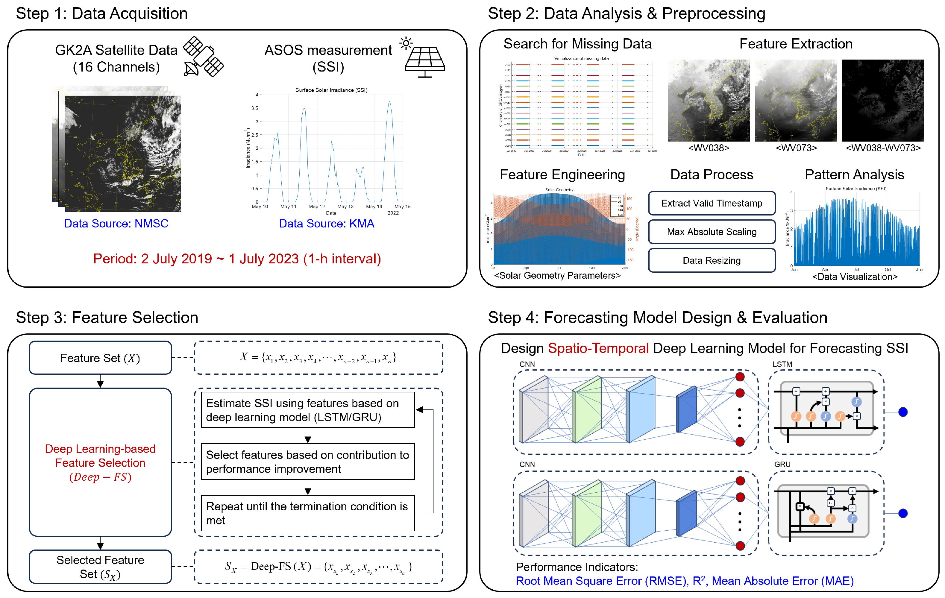
This section presents a step-by-step description of the proposed method for forecasting SSI. Figure 1 shows an overview of the step-by-step procedure of the proposed method, which consists of four steps: data acquisition, data analysis and preprocessing, feature selection, and forecasting model design and evaluation. In the data acquisition step, 16-channel data from the GK2A satellite and SSI data from the ASOS station on the ground are acquired. In the data analysis and preprocessing step, the data are prepared for feature selection and the SSI forecasting model. The data characteristics and patterns are analyzed and subjected to feature extraction and engineering. Additionally, data preprocessing, such as extraction for valid timestamp and region of interest (ROI), normalization, and resizing, is performed. In the feature selection step, feature variables appropriate for SSI forecasting are selected. Deep-FS is applied to the feature variables prepared in the second step to select the feature variables that affect SSI. Finally, in the forecasting model design and evaluation step, the spatio-temporal model for SSI forecasting is designed using the selected feature variables and evaluated. The details of each step are explained individually in separate sections.
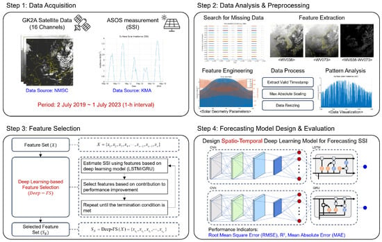
Figure 1.
Overview of the step-by-step procedure of the proposed method consists of four steps: data acquisition, data analysis and preprocessing, feature selection, and forecasting model design and evaluation.
2.1. Data Acquisition
2.1.1. GEO-KOMPSAT-2A (GK2A)
GK2A is a geostationary meteorological satellite of South Korea performing meteorological and space weather observation missions since its launch on 5 December 2018. It is equipped with an advanced meteorological imager (AMI), enabling accurate observation. GK2A utilizes AMI to observe the weather of Earth through 16 channels with different wavelengths: VIS004, VIS005, VIS006, VIS008, NIR013, NIR016, SWIR038, WV063, WV069, WV073, IR087, IR096, IR105, IR112, IR123, and IR133. The 16-channel data for the observations by GK2A are provided after several preprocessing procedures at the National Meteorological Satellite Center (NMSC) in South Korea. Table 2 shows the specifications for the 16 channels of GK2A provided by NMSC. Each of the 16 channels has three observation areas: Full Disk (FD), East Asia (EA), and Korea (KO). The FD area is observed every 10 min, whereas the other areas are observed every 2 min and have high spatial resolutions of 0.5/1.0/2.0 km, depending on the channel [29]. In this study, we used 16-channel data obtained every hour on the hour for the KO area. The period of the acquired data was 2 July 2019, 00:00:00 to 1 July 2023, 00:00:00, based on Korea Standard Time (KST) (hereinafter, these data are referred to as the GK2A dataset).

Table 2.
Data specifications of 16 channels used for observation by AMI mounted on GK2A.
2.1.2. Automated Synoptic Observing System (ASOS)
Synoptic weather observation refers to ground observation conducted simultaneously at all weather stations to determine atmospheric conditions at a given time. Synoptic weather observation automatically observes atmospheric conditions using ASOS, excluding some visual observations such as visibility, cloud forms, and weather phenomena. KMA operates 96 ASOS stations (as of 1 April 2020) and provides various meteorological data such as temperature, precipitation, pressure, and humidity observed on the ground. SSI observation data are provided through the hourly aggregation of SSI measured every minute using pyranometers at ASOS stations. In this study, SSI observation data provided hourly intervals every hour on the hour were collected from the ASOS station (latitude: 35.10468°, longitude: 129.03203°) located in Busan, South Korea. The SSI data were collected from 2 July 2019, 00:00:00 to 1 July 2023, 00:00:00, based on KST (hereinafter, these data are referred to as the SSI dataset).
2.2. Data Analysis & Preprocessing
2.2.1. Search for Missing Values
If an observation or event results in missing data, either the data will not be stored, or meaningless values will be stored. Therefore, a missing value search must be performed before the data are used. For the GK2A dataset, the primary cause of missing data is periodic inspections such as satellite attitude correction. Because missing data are not stored in the GK2A dataset, the missing points can easily be searched by checking the data memory or sorting the data in chronological order. Furthermore, in the SSI dataset, missing data can be due to non-detection of solar irradiance and the occurrence of sensor errors. Because missing data are stored as Not a Number (NaN) in the SSI dataset, points of error/missing values can be found through data exploration. Table 3 shows the results of searching for missing values in the acquired GK2A and SSI datasets. In the GK2A dataset, in most cases, data for each channel are missing owing to satellite maintenance, and the low missing rate is approximately 1.7%. Meanwhile, the SSI dataset appears to have many missing values because the non-detection of solar irradiance after sunset is regarded as missing data. However, considering the number of data corresponding to sunrise to sunset times (16,004), it can be inferred that most of the missing data are not due to sensor errors but, rather, due to unobserved SSI. Although missing values may be interpolated, they are likely to have errors owing to the nature of interpolation. Therefore, this study excluded missing values entirely instead of accepting the errors that are likely to result from interpolating missing values.

Table 3.
Results of searching for missing values in GK2A and SSI datasets.
2.2.2. Analysis of Data Characteristics
The 16 channels in the GK2A dataset are divided into 5 categories: visible channel, near-infrared channel, shortwave infrared channel, water vapor channel, and infrared channel. Each category has common characteristics, and simultaneously, each channel has unique characteristics corresponding to different wavelengths. Therefore, the objects that can be observed are different for each channel. Table 4 shows the characteristics of the 16 channels by category and the observation targets for each channel.

Table 4.
Characteristics of 16 channels by category and observation targets by channel.
The visible channel can be observed only during the day when there is sunlight, and the observed value represents the intensity of sunlight reflected from clouds and the ground surface. Moreover, in the visible channel, the reflected light is proportional to the observed value because the stronger the reflected sunlight, the greater its brightness. The near-infrared channel has a wavelength range in the infrared region with relatively low interference from water vapor. Similar to the visible channel, it is observable only during the day. The shortwave infrared channel can observe solar radiation and earth radiation simultaneously. It is used mainly at night because the reflected solar radiation is stronger than the reflected earth radiation during the day. The water vapor channel is an infrared channel with a wavelength that absorbs water vapor and reacts sensitively to water vapor even in a cloudless atmosphere. Unlike the visible channel, the infrared channel allows observation at night and observes mainly the intensity of energy emitted by the surface of Earth and by objects. The intensity of the emitted energy is determined by temperature, and the object temperature estimated from the infrared channel is called the brightness temperature (BT).
Because the SSI dataset provided by KMA is based on observations through the Solar System by the ASOS station on the ground, it is directly affected by the geometric properties of the sun, such as its position and altitude angle. It is also affected by factors that cause reflection and scattering as sunlight travels to the surface of the atmosphere, such as cloud cover, water vapor, and fog. Therefore, feature variables representing the geometry of the sun and the atmospheric conditions of Earth are needed to forecast SSI. In this context, satellite data of observations of Earth’s weather from outside the Earth are very suitable for SSI forecasting. However, indiscriminate use of data can increase model complexity and result in performance degradation, and thus, it is necessary to subject the data to appropriate data preprocessing, feature extraction, and selection processes. Therefore, we extracted features corresponding to the ROI from the GK2A dataset and performed feature engineering based on solar geometry to consider the geometric properties of the sun. In addition, we used Deep-FS to select feature variables suitable for forecasting SSI.
2.2.3. ROI Extraction and Calibration
The collected SSI dataset comprises 1D data obtained by the ASOS station installed in Busan, South Korea, and thus, the ROI must be extracted from the 2D GK2A dataset for the Korean Peninsula area. We set a rectangular area of 18 km × 18 km as the ROI based on the latitude and longitude coordinates of the ASOS station in Busan and extracted data corresponding to the ROI using the 2D latitude map and 2D longitude map of the GK2A dataset. Because the GK2A dataset is obtained after it is converted to lightweight values for data storage efficiency, it must be converted to physical values for use. Therefore, the visible and near-infrared channel data were calibrated with albedo, whereas the other channel data were calibrated with BT.
2.2.4. Feature Extraction
NMSC generates various meteorological outputs such as clouds, yellow dust, convective clouds, and total cloud cover based on 16-channel data provided by GK2A. Research studies on each output primarily used the channels (Ch07 to Ch16) in the infrared wavelength range, because of which observations could be made even at night. Moreover, apart from the raw data of each channel, the maximum, minimum, average, median, standard deviation and the difference between the maximum and minimum values of the data, etc., within a specific space or time interval were used to generate meteorological outputs. In particular, considering the unique characteristics of each channel, the BT differences between infrared channels were employed as main key feature variables [30]. Therefore, for this study, we extracted all BT differences and ratios between the infrared channels (Ch07 to Ch16) as feature variables. Consequently, we could extract 106 feature variables, including raw data from 16 channels. Table 5 shows each of the 106 feature variables.

Table 5.
Information about 106 feature variables extracted from GK2A dataset.
2.2.5. Feature Engineering
SSI is directly related to the geometric properties of the sun, such as its position and altitude and, therefore, these parameters are essential factors in forecasting SSI. Accordingly, we used solar declination (SD), solar elevation angle (SEA), and ESR among the solar geometry parameters. SD refers to the angle indicating how far the sun is from the declination of Earth (celestial equator), whereas the SEA refers to the height of the sun expressed in degrees relative to the horizon. Meanwhile, ESR refers to the amount of solar irradiance before scattering or absorption by dust or water vapor in the atmosphere. SD, SEA, and ESR were derived using solar geometry formulas [31,32] based on the latitude and longitude of the ASOS station in Busan.
The descriptions of the variables used in the formulas are as follows:
- : Julian Day.
- n: Number of days from J2000.0 (=Julian Day for 1 January 2000 at 12:00 noon).
- L: Mean longitude of the sun corrected for aberration in degrees.
- g: Mean anomaly in degrees.
- : Ecliptic longitude in degrees.
- : Obliquity of the ecliptic in degrees.
- : Declination angle of the sun in degrees.
- : Right ascension in degrees.
- : Equation of time in minute.
- : Time in Coordinated Universal Time (UTC).
- : Longitude of the subsolar point at which the sun is perceived to be directly overhead (at the zenith) in degrees.
- : Latitude in degrees.
- : Longitude in degrees.
- : Solar elevation angle or altitude angle in degrees.
- : Hour angle at sunrise in degrees.
- : Hour angle at sunset in degrees.
- : Day of year (sequential day number starting with day 1 on 1 January).
- : Solar constant (=1367 W/m2).
- : Extraterrestrial solar radiation incident on the plane normal to the radiation on the in W/m2.
- : Hour angle in degrees.
- : Extraterrestrial solar radiation incident on a horizontal plane outside of the atmosphere at in W/m2.
- : Accumulated extraterrestrial solar radiation from to in MJ/m2.
We generated data on the three solar geometry parameters every hour between 2 July 2019, 00:00:00 and 1 July 2023, 00:00:00, based on KST (hereinafter, these data are referred to as the SG dataset). Table 6 shows information about the three solar geometry parameters generated through solar geometry-based feature engineering.

Table 6.
Information about the three solar geometry parameters.
2.2.6. Data Process for Deep Learning
To use a deep learning model, it is necessary to convert the data into a form that fits the input structure of the model. In addition, before training the model, invalid data must be removed and the data must be normalized to prevent the model from falling into local minima or overfitting. Considering the validity of the data, we excluded missing values and extracted data corresponding to meaningful periods based on the hour angles at sunrise () and sunset (). Furthermore, we performed data resizing to unify the data structure according to the input structure of the deep learning model. In the feature selection step, we used data from a time zone that satisfies , covering the range from 2 h after sunrise to 2 h before sunset, to exclude errors in solar geometry and due to SSI observed even after sunset. In addition, for feature selection, we averaged the ROI of the GK2A dataset to transform it into a 1D structure.
In the forecasting model design and evaluation step, we used data from a time zone that satisfies , covering sunrise to sunset. Moreover, to utilize the spatio-temporal deep learning model, we performed data resizing to enforce the same width and height for the ROI, for which we employed a method based on sliding the average window without overlapping. Then, we generated the SG dataset as a 2D structure based on the 2D latitude and longitude map of the GK2A dataset. Moreover, we converted the SD data, which do not use latitude and longitude, via data replication to a 2D structure. Lastly, when training the deep learning model, we performed data normalization to improve learning efficiency and prevent overfitting. We also applied absolute normalization instead of Z-score normalization or 0–1 normalization to maintain the relative size and direction of the data. Equation (17) is the formula used for max absolute scaling.
In this equation, refers to the normalized variable, X refers to the variable before normalization, and refers to the maximum value of the variable.
2.2.7. Data Visualization and Pattern Analysis
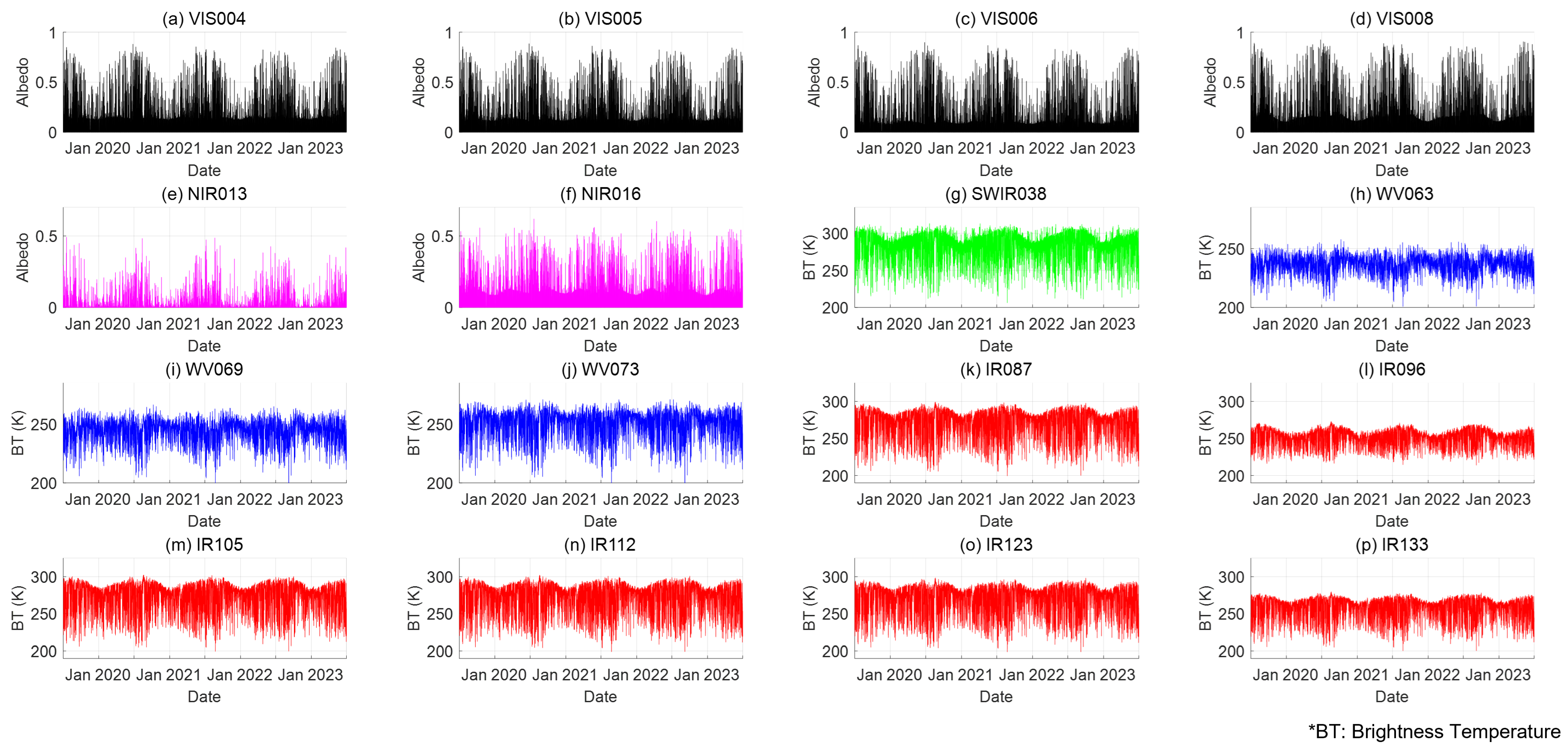
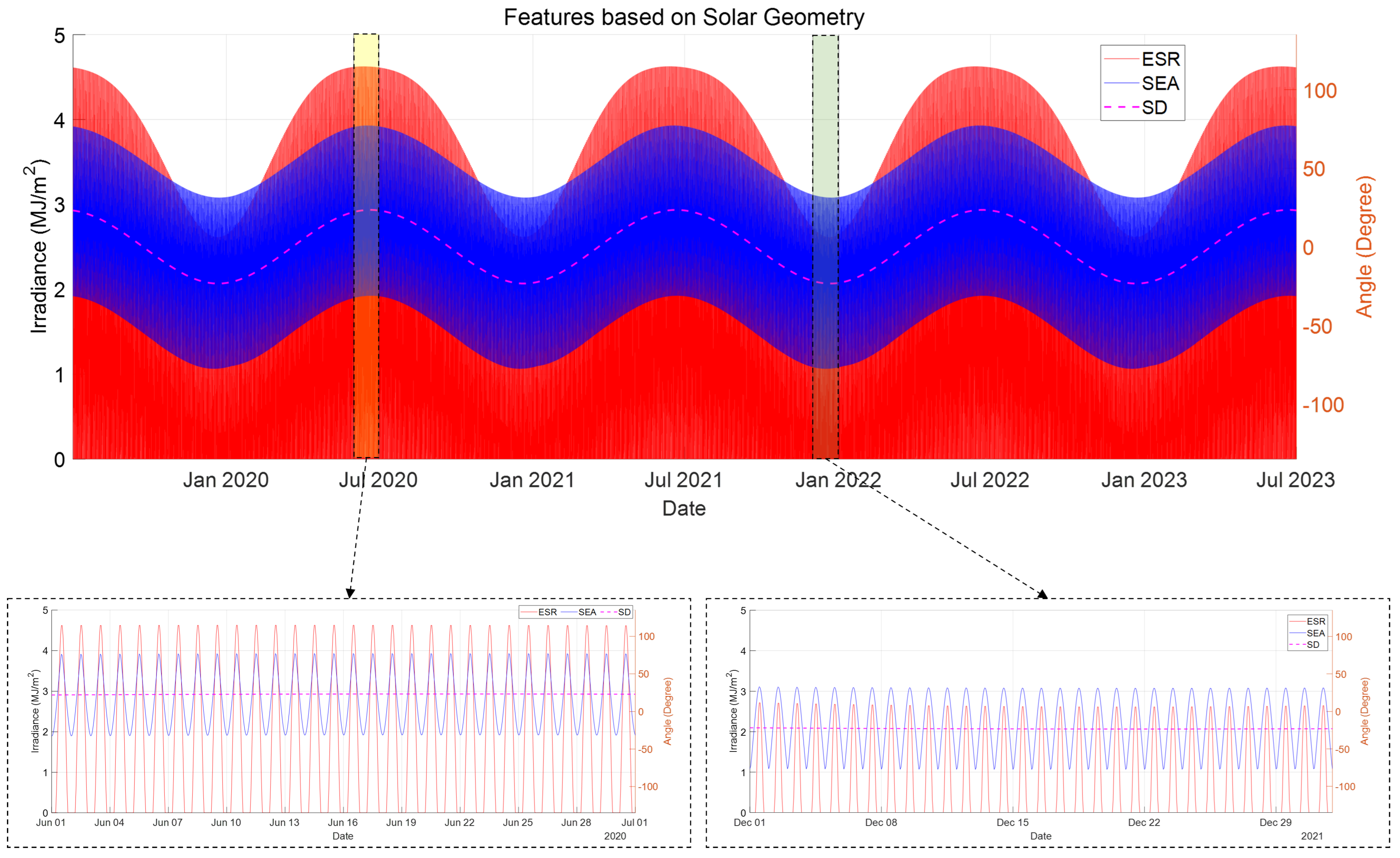
We analyzed the patterns in the acquired data via visualization. For this, we converted the GK2A dataset, which has a 2D structure, to a 1D structure by obtaining the average for the ROI. Figure 2, Figure 3 and Figure 4 show visualizations of the GK2A, SSI, and SG datasets, respectively. Figure 2 confirms that among the 16 channels that constitute the GK2A dataset, channels belonging to the same category have similar patterns, all channels repeat seasonal patterns every year, and the channels that can be observed only during the day and those that can be observed both day and night exhibit clearly different patterns. Figure 3 shows that the pattern of daily maximum SSI increasing and decreasing over a yearly cycle is repeated and that there is severe volatility depending on the time. It can be inferred that this variability is due to weather conditions, and thus, it is necessary to find appropriate features that represent the weather conditions that affect variability. Meanwhile, Figure 4 confirms that the SG dataset is consistent with the geometric properties of the sun over a yearly cycle, ESR is proportional to SEA, and the daily maximum ESR changes depending on SD.

Figure 2.
Visualization of 16-channel data belonging to GK2A dataset.
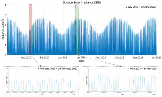
Figure 3.
Visualization of SSI dataset.

Figure 4.
Visualization of SG dataset.
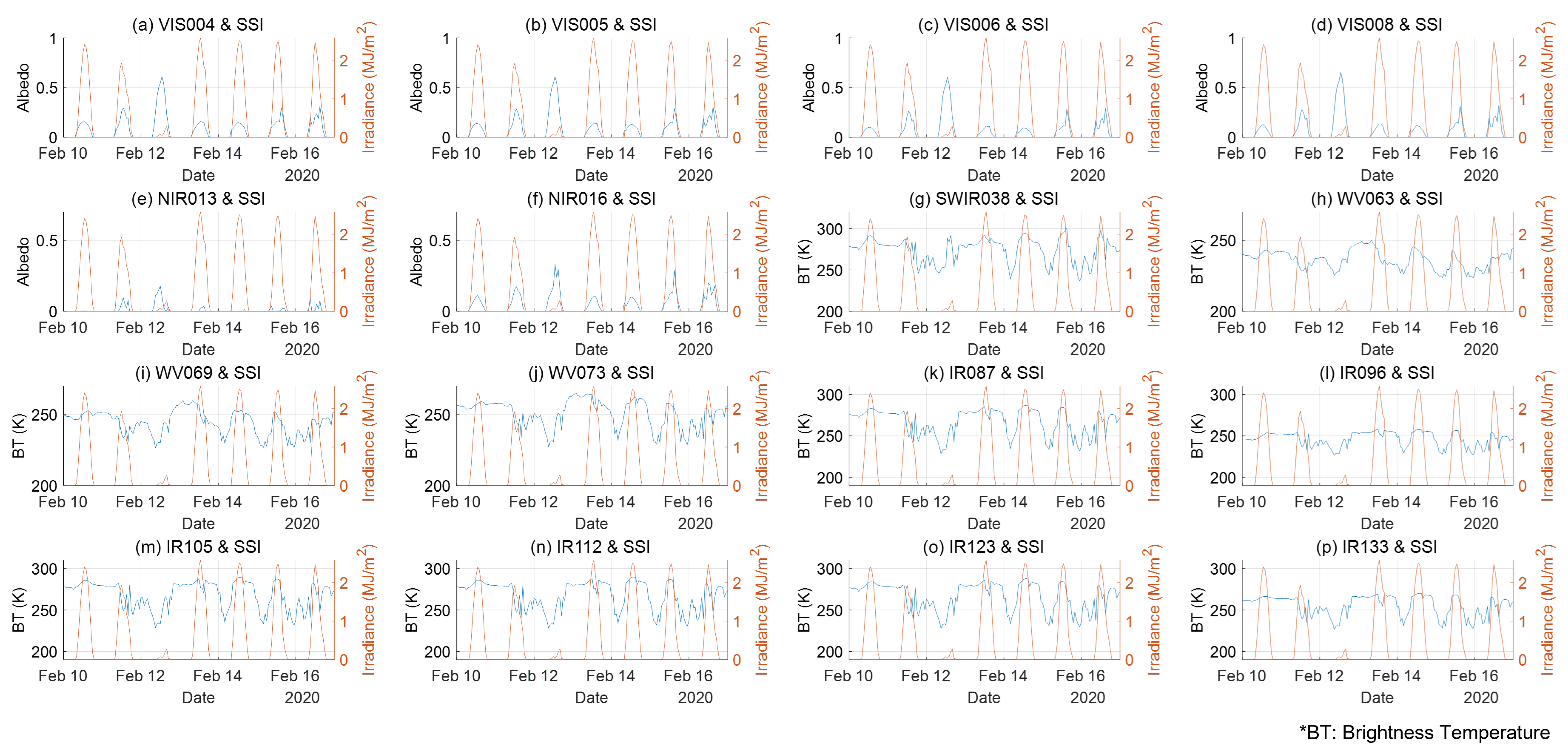
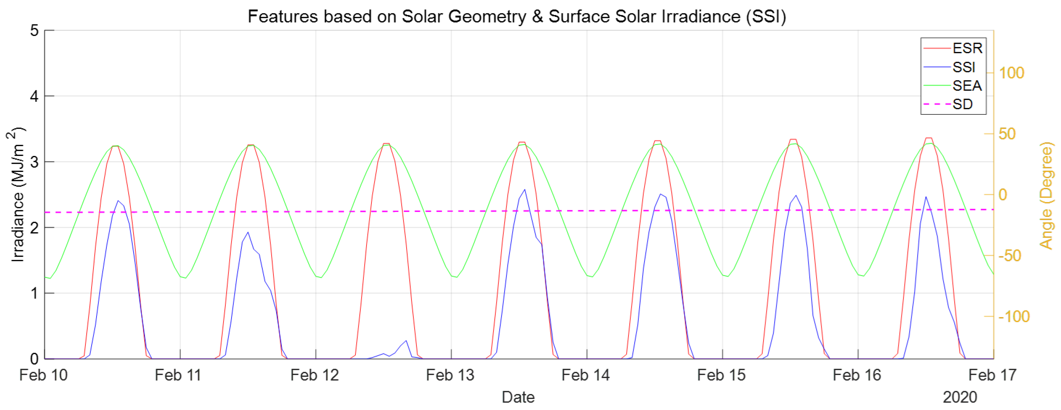
To visually analyze the relationship between the 16-channel data and solar geometry parameters on the SSI, Figure 5 and Figure 6 provide simultaneous visualizations of the data for some of the collected data periods (10 February 2020 to 16 February 2020). Figure 5 shows that although channels belonging to the same category in the GK2A dataset have similar patterns, the channels have detailed differences between them. Moreover, as mentioned earlier, it can be confirmed that the visible and near-infrared channels can be observed only during the day, whereas the other channels can be observed both during the day and at night. The visible channel and near-infrared channels also exhibit a clearly inversely proportional relationship to SSI. This is in contrast to the other channels, for which it is difficult to visually confirm any relationships with SSI. Figure 6 shows that SSI is proportional to SEA and ESR and that the degree to which SSI is attenuated by the atmosphere can be intuitively confirmed. Through data pattern analysis using data visualization, we verified that the SG dataset effectively represents the periodicity and pattern of SSI and judged it to be suitable as a feature for SSI forecasting. In addition, we determined that although some channels clearly show relationships with SSI, there are also channels where no relationships can be visually identified. Therefore, it is necessary to select appropriate features that are influential to SSI.
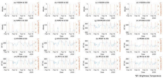
Figure 5.
Visualization overlapping SSI and GK2A datasets over a certain period (10 February 2020 to 16 February 2020).
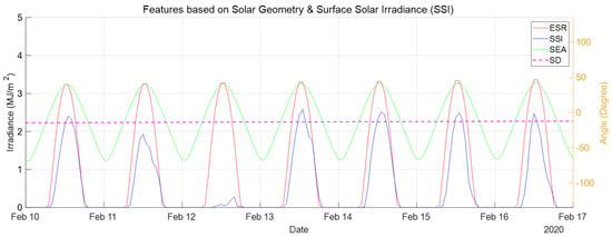
Figure 6.
Visualization overlapping SG and GK2A datasets over a certain period (10 February 2020 to 16 February 2020).
2.3. Feature Selection
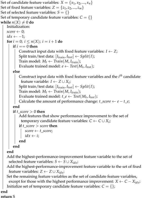
We used Deep-FS to select feature variables that effectively influence SSI among the 106 feature variables derived from the GK2A dataset. The feature selection method imitated the forward selection of the wrapper method, and we assumed a change in SSI estimation performance according to the use or absence of a feature variable with an effect on or correlation with SSI; that is, if the performance is improved using a particular feature variable, it was determined that the feature was related to SSI and could affect SSI. The reason for using Deep-FS for SSI estimation rather than SSI forecasting is to understand the influence of specific feature variables on SSI more clearly. The deep learning models used in Deep-FS are LSTM and GRU, which are specialized for time-series prediction and use an input–output structure in Sequence-to-Sequence (Seq2Seq) form. RMSE was used as the performance indicator. Algorithm 1 provides the pseudocode of Deep-FS.
Because Deep-FS has no limit to the number of variables that it can use as input, it can provide other information, such as time and location, to clarify the correlation or influence of feature variables on the target variable. Additionally, it can be used to identify any linear and non-linear relationships between two variables. Taking advantage of this, we used not only SSI at the previous point in time but also the three solar geometry parameters and feature variables corresponding to the visible channel as fixed input variables. Then, we employed Deep-FS on the remaining 102 feature variables as candidate feature variables. Moreover, when the 106 feature variables derived from the GK2A dataset were used, 2D data corresponding to the ROI were averaged and converted into 1D. Table 7 shows the information on the model structure, input variables, output variables, and input/output (I/O) time stamps used in Deep-FS.

Table 7.
Information about model structure, input variables, output variables, and I/O timestamp used in Deep-FS: N = number of input variables, S = sequence length, ssi = SSI.
The number of layers and nodes of the deep learning model used in Deep-FS was determined through repeated experiments with various values. Given that the SSI is 1-h accumulated solar irradiance, both timestamp and t were used to estimate SSI at timestamp t in the case of the SG and GK2A datasets, which comprise instantaneous values. Moreover, as mentioned earlier, to exclude errors in solar geometry and owing to SSI observed even after sunset, data from a period that satisfies , covering the range from 2 h after sunrise to 2 h before sunset, were used. Given the Seq2Seq type I/O structure, a sequence for the unbroken, continuous data section was also formed. For the performance evaluation, the training and evaluation process was repeated five times, considering the randomness of the deep learning model, and the lowest RMSE was considered the final measure of performance. Subsequently, we designed an SSI forecasting model based on the features selected through Deep-FS. Details about this model will be discussed in Section 2.4.
2.4. Forecasting Model Design & Evaluation
We used a spatio-temporal deep learning model that combines a CNN model specialized for extracting the spatial features of 2D data and an LSTM or GRU model specialized for predicting time-series data to reflect the temporal and spatial characteristics of SSI. The I/O structure of the model used the Seq2Seq format. Moreover, the input variables of the model used N feature variables (), three solar geometry parameters (), and four visible-channel feature variables () selected in the feature selection step. For all input variables, preprocessed data in a size for an 18 km × 18 km area based on the latitude and longitude coordinates of the ASOS station in Busan, where the SSI is measured, were used. Table 8 shows the structure, input variables, output variables, and I/O timestamp of the designed SSI forecasting model.

Table 8.
Structure, input variables, output variables, and I/O timestamp of designed SSI forecasting model: N = number of input variables, S = sequence length, ssi = SSI.
The structure and hyperparameters (number of layers, number of nodes, filter size, number of filters, stride, etc.) of the deep learning model used to forecast SSI were determined through repeated experiments with various values as in feature selection. To forecast the SSI after 1 h (), the visible-channel feature variables of the current time (t) and the selected feature variables were used. In the case of the SG dataset, with which we can determine the future through solar geometry, the timestamps t and were employed. To use only data from a valid section for forecasting SSI, data from a time zone that satisfies , covering the range from sunrise to sunset, were targeted. Furthermore, given the Seq2Seq type I/O structure, a sequence was formed for the unbroken, continuous data section and used for I/O. For the performance evaluation, the training and evaluation process was repeated five times, considering the randomness of the deep learning model. Then, RMSE, RRMSE, R2, and MAE were obtained based on the model with the lowest RMSE.
| Algorithm 1: Deep Learning-based Feature Selection (Deep-FS). |
 |
3. Experimental Results
We performed various comparison experiments to verify the performance of the proposed method. For the experiments using the deep learning model, the model was trained using the training options outlined in Table 9. Three years of data was used to train the model, whereas six months of data was used to validate and test the model. We applied early stopping constraints to avoid long training times and prevent overfitting of the model. Additionally, based on the loss of verification data recorded in each verification cycle, the model at the point in time with the lowest verification loss was made the final output. The performance of the proposed method was verified against those of other methods in terms of the following aspects:

Table 9.
Description of data and training options for the experiments using the deep learning model.
- Performance comparison between using feature variables selected through Deep-FS and that through conventional feature selection methods.
- Performance comparison between spatio-temporal models (CNN-LSTM, CNN-GRU) and single models (ANN, CNN, LSTM, GRU).
- Performance comparison depending on the use of the SG dataset.
First, we performed an experiment to verify that Deep-FS is superior to traditional feature selection methods. The feature selection methods included in this experiment were filter methods based on the PCC and minimum redundancy maximum relevance (mRMR). The first filter method selected the top 5%, 10%, and 15% features based on the PCC, which indicates the strength of the linear relationship, whereas the second filter method, based on the mRMR, selected the top 5%, 10%, and 15% of features based on feature importance. The case wherein all feature variables were used was also considered. Table 10 shows the feature variables selected according to the feature selection methods.

Table 10.
Feature variables selected by feature selection methods.
Table 11 shows the results of spatio-temporal deep learning model-based SSI forecasting experiment using feature variables selected by each feature selection method and solar geometry parameters as input variables. In Table 11, Deep-FS (LSTM) refers to LSTM-based Deep-FS, whereas Deep-FS (GRU) refers to GRU-based Deep-FS and the best performers for each metric are highlighted in bold blue text. As shown in Table 11, using Deep-FS leads to superior SSI forecasting performance compared to using all feature variables or conventional feature selection methods in all performance indicators. When comparing feature selection methods based on PCC, the results showed that PCC Top 15% > PCC Top 10% > PCC Top 5% in terms of higher performance, indicating that using more variables with higher Pearson correlation coefficients improved performance. Similarly, when comparing feature selection methods based on mRMR, the results showed that mRMR Top 15% > mRMR Top 10% > mRMR Top 5% in terms of higher performance, indicating that using more variables with higher feature importance improved performance. And when comparing feature selection methods based on Deep-FS, the results showed that the Deep-FS using GRU slightly outperformed.

Table 11.
Experimental results comparing the performance of SSI forecasting across different feature selection methods.
Based on experimental results, the feature selection methods could be ranked from highest to lowest performance as follows: Deep-FS (GRU) > Deep-FS (LSTM) > mRMR Top 10% > mRMR Top 5% > mRMR Top 15% > All > PCC Top 15% > PCC Top 10% > PCC Top 5%. The feature selection method based on PCC is inferred to have low performance because it not only identifies linear relationships between only 1:1 features but also fails to consider redundancy. However, when all features are used, low performance is likely to result from not only increasing the complexity of the model but also requiring sufficient data for training as the number of parameters to be trained increases exponentially. Meanwhile, mRMR can select important features by minimizing the amount of mutual information (redundancy) between features and maximizing the correlation (relevance) with target variables. However, it does not consider non-linear relationships and therefore leads to a lower performance than that of the proposed Deep-FS.
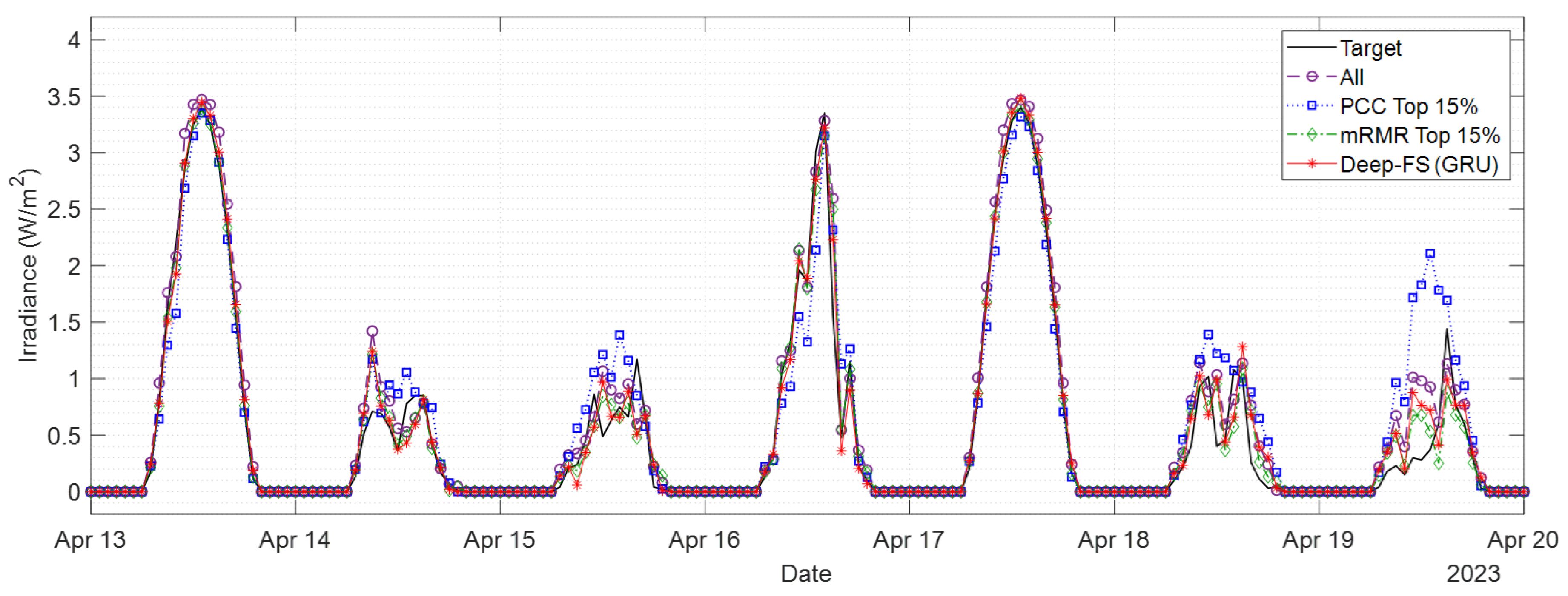
Figure 7 shows the results of forecasting SSI 1 h ahead in a certain period (13 April 2023, 00:00:00 to 20 April 2023, 00:00:00) using the CNN-LSTM-based SSI forecasting models utilized four feature selection methods (All, PCC Top 15%, mRMR Top 15%, Deep-FS (GRU)), which showed high performance in each method. From Figure 7, it can be inferred that 13 and 17 April are sunny, 6 April is partly cloudy, and the rest of 14–15 and 18–19 April are cloudy. On sunny days, the forecasting performed well overall for all models. However, on cloudy days, the difference in forecasting performance for each feature selection method is intuitively apparent. It can be seen that the model utilizing the PCC Top 15% has a larger scale of over-forecasting or under-forecasting compared to the models utilizing other feature selection methods, and it does not track the increase/decrease trends well. On the other hand, models utilizing feature selection methods except for PCC Top 15% have similar abilities to track increase/decrease trends. Still, there are slight differences in the scale of over-forecasting or under-forecasting.
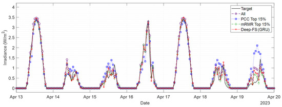
Figure 7.
Experimental results of forecasting SSI 1 h ahead in period (13 April 2023, 00:00:00 to 20 April 2023, 00:00:00) using the CNN-LSTM-based SSI forecasting models utilized four feature selection methods: All, PCC Top 15%, mRMR Top 15%, and Deep-FS (GRU).
Afterward, an experiment was conducted to compare the performance of the proposed spatio-temporal deep learning model against those of single deep learning models to verify if simultaneously accounting for both temporal and spatial elements leads to better performance. The comparison models included in this experiment were ANN, CNN, LSTM, and GRU, and the input variables were feature variables selected via Deep-FS and the solar geometry parameters. Table 12 shows experimental results comparing the performance of the deep learning models, where all the models used feature variables selected by Deep-FS. The top performers for each metric are highlighted in bold blue text. As shown in Table 12, it can be confirmed that the proposed spatio-temporal deep learning models (CNN-LSTM, CNN-GRU) performed better than the single deep learning models (ANN, CNN, LSTM, GRU).

Table 12.
Experimental results comparing the performance of SSI forecasting across different deep learning models.
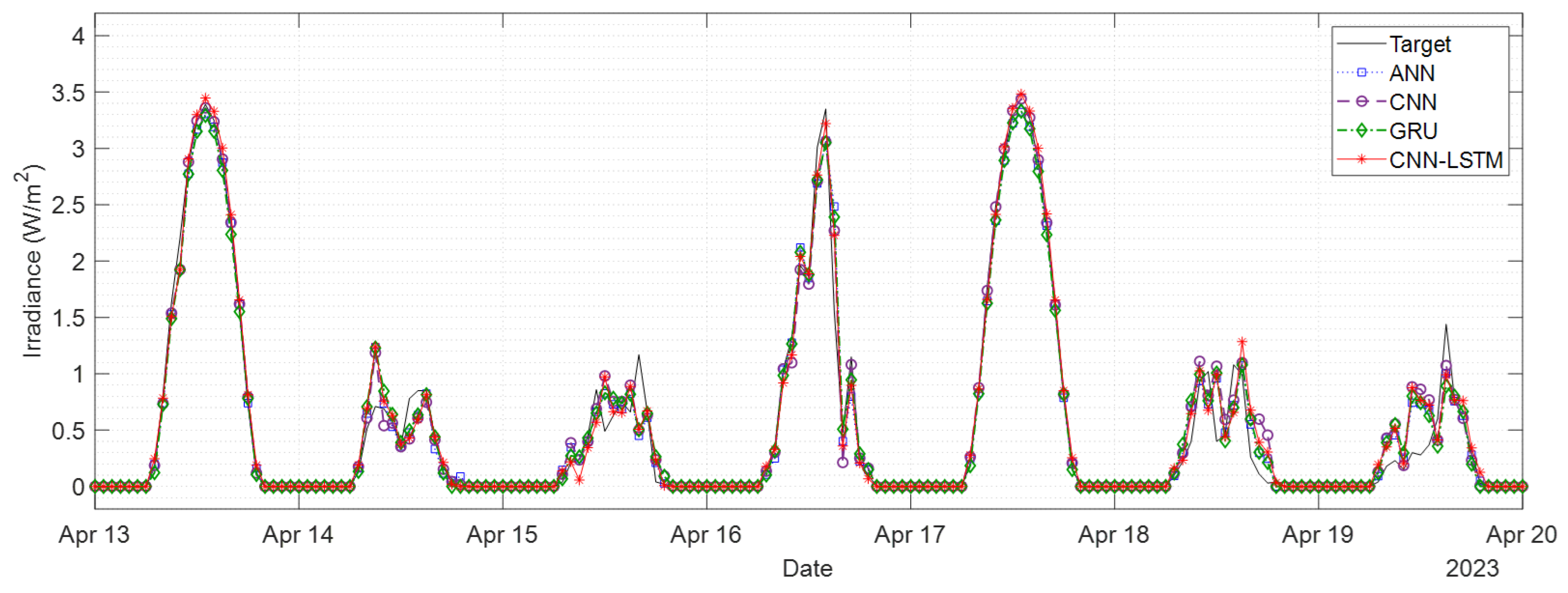
Based on experimental results, forecasting models could be ranked from highest to lowest performance as follows: CNN-LSTM > CNN-GRU > GRU > LSTM > CNN > ANN. Because SSI data are inherently time series, we found that GRU and LSTM, models that specialize in predicting time series data, performed better than CNN and ANN. In the case of the CNN model, it cannot reflect the time series characteristic in the same way as ANN, but it can reflect spatial characteristic, which is why they seem to perform better than ANN. On the other hand, spatio-temporal deep learning models (CNN-LSTM, CNN-GRU) are believed to have better performance than single deep learning models (ANN, CNN, LSTM, GRU) because they can consider temporal and spatial characteristics simultaneously. Figure 8 shows the results of forecasting SSI 1 h ahead in a certain period (13 April 2023, 00:00:00 to 20 April 2023, 00:00:00) utilized the four SSI forecasting models (ANN, CNN, GRU, CNN-LSTM) using selected feature variables based on Deep-FS (GRU) and SG parameters as input. Overall, we found that the ability to track SSI’s upward and downward trend was similar regardless of weather conditions in all models. Still, there are slight differences in the scale of over-forecasting or under-forecasting.
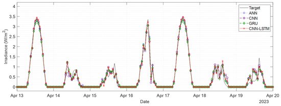
Figure 8.
Experimental results of forecasting SSI 1 h ahead in period (13 April 2023, 00:00:00 to 20 April 2023, 00:00:00) with four forecasting models (ANN, CNN, GRU, CNN-LSTM) using SG parameters and feature variables selected based on Deep-FS (GRU) as input variables.
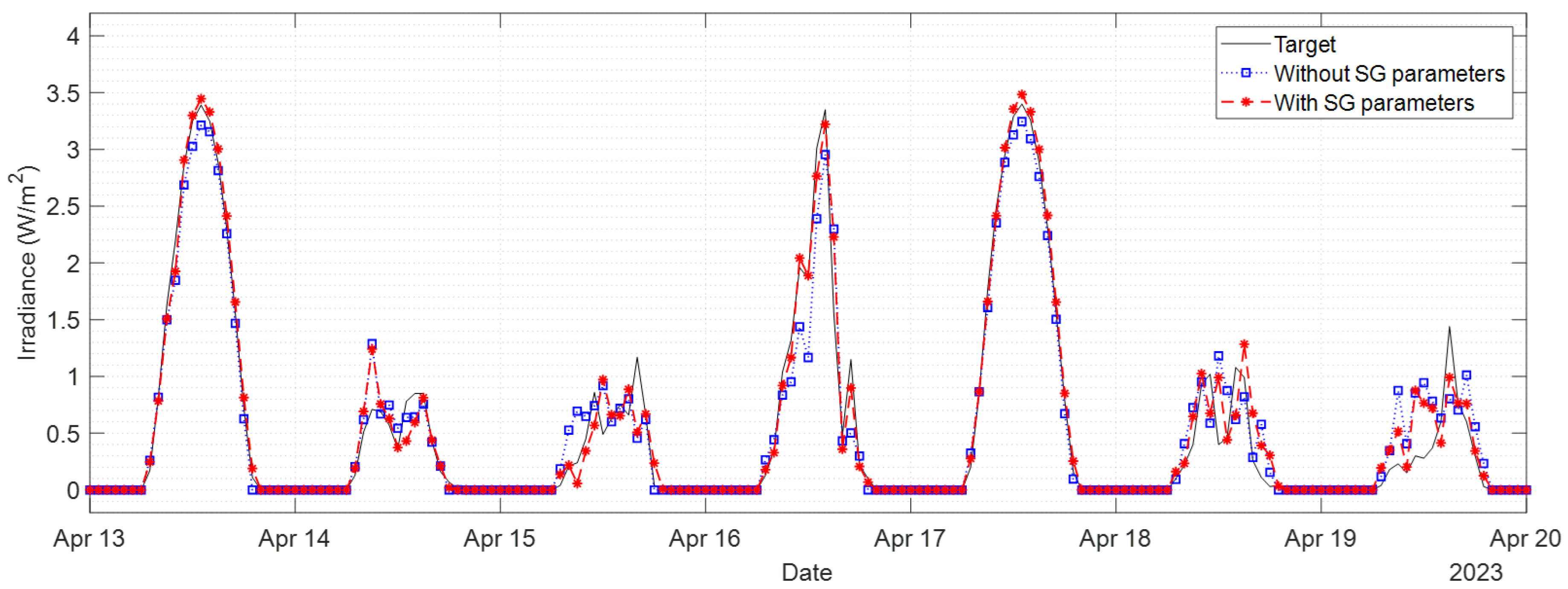
Lastly, to verify the effectiveness of the solar geometry parameters (SD, SEA, ESR), we conducted an experiment to compare model performance depending on whether these parameters were used as input variables. The forecasting models included in this experiment were ANN, CNN, LSTM, GRU, CNN-LSTM, and CNN-GRU, and the feature variables were selected using Deep-FS. Table 13 shows the results of comparative experiments between the models that used the solar geometry parameters and those that did not. The table highlights the best performers for each metric with blue and bold text. As a result, it was found that performance is significantly improved when solar geometry parameters are included among the input variables, regardless of the model used. The reason for this is believed to be that solar geometry parameters not only reflect the periodic pattern characteristics of SSI but also allow future values to be calculated in advance through solar geometry. Thus, it was confirmed that the parameters engineered based on solar geometry contributed decisively to improving SSI forecasting performance. Figure 9 shows the results of forecasting SSI 1 h ahead with and without SG parameters as input variables in a certain period (13 April 2023, 00:00:00 to 20 April 2023, 00:00:00) using the CNN-LSTM model utilized Deep-FS (GRU). While there is not much difference in following SSI’s up and down trend, it is confirmed that using the SG parameter effectively improves over-forecasting and under-forecasting regardless of the weather.

Table 13.
Experimental results comparing the performance of SSI forecasting with and without SG parameters.
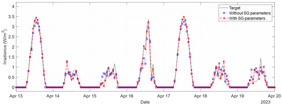
Figure 9.
Experimental results of forecasting SSI 1 h ahead with and without SG parameters as input variables in a certain period (13 April 2023, 00:00:00 to 20 April 2023, 00:00:00) using the CNN-LSTM model utilized Deep-FS (GRU).
4. Conclusions
In this study, we investigated and developed a method for forecasting SSI 1 h in advance using imageries of 16 channels observed from the GK2A satellite as the primary data. To account for fundamental factors, such as the position of the sun, that affect SSI, we used solar geometry to engineer feature variables such as SD, SEA, and ESR. Additionally, to prevent model performance degradation due to indiscriminate use of feature variables, appropriate feature variables for SSI forecasting were selected using Deep-FS. We also designed a spatio-temporal deep learning model that combines a CNN, which can extract spatial features, and an LSTM or GRU, which are specialized for forecasting time-series data. For verification, we compared the proposed method with traditional methods based on three performance indicators (RMSE, RRMSE, R2, MAE). Our experimental results show that the proposed spatio-temporal deep learning model (CNN-LSTM, CNN-GRU) delivers superior overall performance to those of ANN, CNN, LSTM, and GRU. Moreover, it was confirmed that features selected using the proposed Deep-FS lead to higher forecasting performance than that produced by features selected via the conventional method. Lastly, it was confirmed that when three solar geometry parameters (SD, SEA, ESR) are used in SSI forecasting, the performance is significantly improved regardless of the forecasting model. Therefore, it was demonstrated that the proposed method could select features appropriate for SSI forecasting and simultaneously exhibit high performance. Furthermore, because this study uses GK2A satellite data as the main data, it can be easily used for any region in the observation area of the satellite. In other words, it is free from locational constraints within the observation area of the satellite.
The limitation of this study is that because the experiment was conducted based on a single ASOS station, geographic factors such as location and topography were not evenly reflected, and there were insufficient data for training because not much time has elapsed yet since the start date of the GK2A mission. In addition, to effectively verify the performance of the proposed method, this study forecasted SSI after 1 h, which is a relatively short time. Accordingly, in future works, we plan to use data from as many ASOS stations as possible to engineer features that can reflect geographical factors. Through this, we will research SSI estimation and forecasting that can simultaneously account for temporal, spatial, and geographical factors. We will also be working on using data that has information about the future, such as weather forecasts or numerical weather prediction models, to forecast SSI over a longer time horizon.
Author Contributions
Conceptualization, J.K. and E.K.; methodology, J.K. and E.K.; software, J.K.; validation, J.K., E.K. and B.K.; formal analysis, J.K., S.J. and M.K.; investigation, J.K., S.J. and M.K.; resources, J.K., M.K. and B.K.; data curation J.K. and B.K.; writing—original draft preparation, J.K.; writing—review and editing, J.K., E.K. and S.K.; visualization, J.K. and M.K.; supervision, S.K.; project administration, S.K.; funding acquisition, S.K. All authors have read and agreed to the published version of the manuscript.
Funding
This work was supported by the Technological Innovation R&D Program (S3238625) funded by the Ministry of SMEs and Startups (MSS, Korea).
Data Availability Statement
GK2A Imagery data used in this study are available at http://datasvc.nmsc.kma.go.kr/datasvc/html/main/main.do?lang=en (accessed on 1 December 2023). In situ SSI measurements by the ASOS station operated by KMA that were used in this study are available at https://data.kma.go.kr/cmmn/main.do (accessed on 1 December 2023).
Conflicts of Interest
The authors declare no conflicts of interest.
Abbreviations
| PV | Photovoltaic |
| GHI | Global horizontal irradiance |
| DHI | Diffuse horizontal irradiance |
| DNI | Direct normal irradiance |
| ARMA | Autoregressive moving average |
| ARIMA | Autoregressive integrated moving average |
| SARIMA | Seasonal autoregressive integrated moving average |
| RF | Random forest |
| SVR | Support vector regression |
| ANN | Artificial neural network |
| LSTM | Long short-term memory |
| GRU | Gated recurrent unit |
| CNN | Convolutional neural networks |
| MAE | Mean absolute error |
| RMSE | Root mean square error |
| MBE | Mean bias error |
| NMAE | Normalized mean absolute error |
| NRMSE | Normalized root mean square error |
| BP | Back propagation network |
| LightGBM | Light gradient boosting machine |
| ESR | Extra-terrestrial solar radiation |
| SHAP | Shapley additive explanation |
| Bi-LSTM | Bi-directional LSTM |
| WPD | Wavelet packet decomposition |
| MLP | Multi-layer perceptron |
| CAL | Effective cloud albedo |
| ConvLSTM | Convolutional long short-term memory |
| ST-GCN | Spatio-temporal graph convolutional network |
| Conv1D | One-dimensional convolution layer |
| Bi-GRU | Bi-directional gated recurrent unit |
| SAM | Self-attention mechanism |
| PCC | Pearson correlation coefficient |
| SCC | Spearman correlation coefficient |
| SSI | Surface solar irradiance |
| GK2A | GEO-KOMPSAT-2A |
| ASOS | Automated synoptic observing system |
| KMA | Korea Meteorological Administration |
| Deep-FS | Deep learning-based feature selection |
| RRMSE | Relative root mean square error |
| R2 | Coefficient of determination |
| ROI | Region of interest |
| AMI | Advanced meteorological imager |
| NMSC | National Meteorological Satellite Center |
| FD | Full Disk |
| EA | East Asia |
| KO | Korea |
| KST | Korea Standard Time |
| NaN | Not a Number |
| BT | Brightness temperature |
| SD | Solar declination |
| SEA | Solar elevation angle |
| SG | Solar geometry |
| UTC | Time in Coordinated Universal Time |
| Seq2Seq | Sequence-to-Sequence |
| I/O | Input/Output |
| Adam | Adaptive moment estimation |
| mRMR | Minimum redundancy maximum relevance |
Appendix A
The formulas for the four metrics used in this paper are shown below: RMSE, RRMSE, R2, and MAE. In Formulas (A1)–(A4), n means the number of data, means the ith target data, means the ith forecasted data (or output data), and implies the average of the target data.
References
- Li, P.; Zhou, K.; Lu, X.; Yang, S. A hybrid deep learning model for short-term PV power forecasting. Appl. Energy 2020, 259, 114216. [Google Scholar] [CrossRef]
- Wang, K.; Qi, X.; Liu, H. Photovoltaic power forecasting based LSTM-Convolutional Network. Energy 2019, 189, 116225. [Google Scholar] [CrossRef]
- Mayer, M.J.; Gróf, G. Extensive comparison of physical models for photovoltaic power forecasting. Appl. Energy 2021, 283, 116239. [Google Scholar] [CrossRef]
- Wang, K.; Qi, X.; Liu, H. A comparison of day-ahead photovoltaic power forecasting models based on deep learning neural network. Appl. Energy 2019, 251, 113315. [Google Scholar] [CrossRef]
- Kim, B.; Suh, D.; Otto, M.O.; Huh, J.S. A novel hybrid spatio-temporal forecasting of multisite solar photovoltaic generation. Remote Sens. 2021, 13, 2605. [Google Scholar] [CrossRef]
- Kim, M.; Song, H.; Kim, Y. Direct short-term forecast of photovoltaic power through a comparative study between COMS and Himawari-8 meteorological satellite images in a deep neural network. Remote Sens. 2020, 12, 2357. [Google Scholar] [CrossRef]
- Chuluunsaikhan, T.; Kim, J.H.; Shin, Y.; Choi, S.; Nasridinov, A. Feasibility Study on the Influence of Data Partition Strategies on Ensemble Deep Learning: The Case of Forecasting Power Generation in South Korea. Energies 2022, 15, 7482. [Google Scholar] [CrossRef]
- Fernandez-Jimenez, L.A.; Muñoz-Jimenez, A.; Falces, A.; Mendoza-Villena, M.; Garcia-Garrido, E.; Lara-Santillan, P.M.; Zorzano-Alba, E.; Zorzano-Santamaria, P.J. Short-term power forecasting system for photovoltaic plants. Renew. Energy 2012, 44, 311–317. [Google Scholar] [CrossRef]
- Hossain, M.S.; Mahmood, H. Short-term photovoltaic power forecasting using an LSTM neural network and synthetic weather forecast. IEEE Access 2020, 8, 172524–172533. [Google Scholar] [CrossRef]
- Yang, D.; Jirutitijaroen, P.; Walsh, W.M. Hourly solar irradiance time series forecasting using cloud cover index. Sol. Energy 2012, 86, 3531–3543. [Google Scholar] [CrossRef]
- Colak, I.; Yesilbudak, M.; Genc, N.; Bayindir, R. Multi-period prediction of solar radiation using ARMA and ARIMA models. In Proceedings of the 2015 IEEE 14th International Conference on Machine Learning and Applications (ICMLA), Miami, FL, USA, 9–11 December 2015; pp. 1045–1049. [Google Scholar]
- Hussain, S.; Al Alili, A. Day ahead hourly forecast of solar irradiance for Abu Dhabi, UAE. In Proceedings of the 2016 IEEE Smart Energy Grid Engineering (SEGE), Oshawa, ON, Canada, 21–24 August 2016; pp. 68–71. [Google Scholar]
- Alharbi, F.R.; Csala, D. A Seasonal Autoregressive Integrated Moving Average with Exogenous Factors (SARIMAX) Forecasting Model-Based Time Series Approach. Inventions 2022, 7, 94. [Google Scholar] [CrossRef]
- Urraca, R.; Antonanzas, J.; Alia-Martinez, M.; Martinez-de Pison, F.; Antonanzas-Torres, F. Smart baseline models for solar irradiation forecasting. Energy Convers. Manag. 2016, 108, 539–548. [Google Scholar] [CrossRef]
- Yang, X.; Ji, Y.; Wang, X.; Niu, M.; Long, S.; Xie, J.; Sun, Y. Simplified Method for Predicting Hourly Global Solar Radiation Using Extraterrestrial Radiation and Limited Weather Forecast Parameters. Energies 2023, 16, 3215. [Google Scholar] [CrossRef]
- Brahma, B.; Wadhvani, R. Solar irradiance forecasting based on deep learning methodologies and multi-site data. Symmetry 2020, 12, 1830. [Google Scholar] [CrossRef]
- Huang, X.; Li, Q.; Tai, Y.; Chen, Z.; Zhang, J.; Shi, J.; Gao, B.; Liu, W. Hybrid deep neural model for hourly solar irradiance forecasting. Renew. Energy 2021, 171, 1041–1060. [Google Scholar] [CrossRef]
- Rajagukguk, R.A.; Kamil, R.; Lee, H.J. A deep learning model to forecast solar irradiance using a sky camera. Appl. Sci. 2021, 11, 5049. [Google Scholar] [CrossRef]
- Nielsen, A.H.; Iosifidis, A.; Karstoft, H. IrradianceNet: Spatiotemporal deep learning model for satellite-derived solar irradiance short-term forecasting. Sol. Energy 2021, 228, 659–669. [Google Scholar] [CrossRef]
- Niu, T.; Li, J.; Wei, W.; Yue, H. A hybrid deep learning framework integrating feature selection and transfer learning for multi-step global horizontal irradiation forecasting. Appl. Energy 2022, 326, 119964. [Google Scholar] [CrossRef]
- Qing, X.; Niu, Y. Hourly day-ahead solar irradiance prediction using weather forecasts by LSTM. Energy 2018, 148, 461–468. [Google Scholar] [CrossRef]
- Wojtkiewicz, J.; Hosseini, M.; Gottumukkala, R.; Chambers, T.L. Hour-ahead solar irradiance forecasting using multivariate gated recurrent units. Energies 2019, 12, 4055. [Google Scholar] [CrossRef]
- Jalali, S.M.J.; Ahmadian, S.; Kavousi-Fard, A.; Khosravi, A.; Nahavandi, S. Automated deep CNN-LSTM architecture design for solar irradiance forecasting. IEEE Trans. Syst. Man, Cybern. Syst. 2021, 52, 54–65. [Google Scholar] [CrossRef]
- Zang, H.; Liu, L.; Sun, L.; Cheng, L.; Wei, Z.; Sun, G. Short-term global horizontal irradiance forecasting based on a hybrid CNN-LSTM model with spatiotemporal correlations. Renew. Energy 2020, 160, 26–41. [Google Scholar] [CrossRef]
- Jebli, I.; Belouadha, F.Z.; Kabbaj, M.I.; Tilioua, A. Prediction of solar energy guided by pearson correlation using machine learning. Energy 2021, 224, 120109. [Google Scholar] [CrossRef]
- Husein, M.; Chung, I.Y. Day-ahead solar irradiance forecasting for microgrids using a long short-term memory recurrent neural network: A deep learning approach. Energies 2019, 12, 1856. [Google Scholar] [CrossRef]
- Yang, D.; Ye, Z.; Lim, L.H.I.; Dong, Z. Very short term irradiance forecasting using the lasso. Sol. Energy 2015, 114, 314–326. [Google Scholar] [CrossRef]
- Castangia, M.; Aliberti, A.; Bottaccioli, L.; Macii, E.; Patti, E. A compound of feature selection techniques to improve solar radiation forecasting. Expert Syst. Appl. 2021, 178, 114979. [Google Scholar] [CrossRef]
- Jang, J.C.; Sohn, E.H.; Park, K.H. Estimating hourly surface solar irradiance from GK2A/AMI data using machine learning approach around Korea. Remote Sens. 2022, 14, 1840. [Google Scholar] [CrossRef]
- Lee, S.; Choi, J. Daytime cloud detection algorithm based on a multitemporal dataset for GK-2A imagery. Remote Sens. 2021, 13, 3215. [Google Scholar] [CrossRef]
- Zhang, T.; Stackhouse, P.W., Jr.; Macpherson, B.; Mikovitz, J.C. A solar azimuth formula that renders circumstantial treatment unnecessary without compromising mathematical rigor: Mathematical setup, application and extension of a formula based on the subsolar point and atan2 function. Renew. Energy 2021, 172, 1333–1340. [Google Scholar] [CrossRef]
- Duffie, J.A.; Beckman, W.A. Solar Engineering of Thermal Processes; John Wiley & Sons: Hoboken, NJ, USA, 2013. [Google Scholar]
Disclaimer/Publisher’s Note: The statements, opinions and data contained in all publications are solely those of the individual author(s) and contributor(s) and not of MDPI and/or the editor(s). MDPI and/or the editor(s) disclaim responsibility for any injury to people or property resulting from any ideas, methods, instructions or products referred to in the content. |
© 2024 by the authors. Licensee MDPI, Basel, Switzerland. This article is an open access article distributed under the terms and conditions of the Creative Commons Attribution (CC BY) license (https://creativecommons.org/licenses/by/4.0/).

