Abstract
Fractional vegetation cover (FVC) is an essential metric for valuating ecosystem health and soil erosion. Traditional ground-measuring methods are inadequate for large-scale FVC monitoring, while remote sensing-based estimation approaches face issues such as spatial scale discrepancies between ground truth data and image pixels, as well as limited sample representativeness. This study proposes a method for FVC estimation integrating uncrewed aerial vehicle (UAV) and satellite imagery using machine learning (ML) models. First, we assess the vegetation extraction performance of three classification methods (OBIA-RF, threshold, and K-means) under UAV imagery. The optimal method is then selected for binary classification and aggregated to generate high-accuracy FVC reference data matching the spatial resolutions of different satellite images. Subsequently, we construct FVC estimation models using four ML algorithms (KNN, MLP, RF, and XGBoost) and utilize the SHapley Additive exPlanation (SHAP) method to assess the impact of spectral features and vegetation indices (VIs) on model predictions. Finally, the best model is used to map FVC in the study region. Our results indicate that the OBIA-RF method effectively extract vegetation information from UAV images, achieving an average precision and recall of 0.906 and 0.929, respectively. This method effectively generates high-accuracy FVC reference data. With the improvement in the spatial resolution of satellite images, the variability of FVC data decreases and spatial continuity increases. The RF model outperforms others in FVC estimation at 10 m and 20 m resolutions, with R2 values of 0.827 and 0.929, respectively. Conversely, the XGBoost model achieves the highest accuracy at a 30 m resolution, with an R2 of 0.847. This study also found that FVC was significantly related to a number of satellite image VIs (including red edge and near-infrared bands), and this correlation was enhanced in coarser resolution images. The method proposed in this study effectively addresses the shortcomings of conventional FVC estimation methods, improves the accuracy of FVC monitoring in soil erosion areas, and serves as a reference for large-scale ecological environment monitoring using UAV technology.
1. Introduction
Vegetation, as an integral component of terrestrial ecosystems, plays a key role in maintaining biodiversity, providing food, containing water, and sequestrating carbon [1]. Nevertheless, soil erosion has become a serious problem worldwide that poses great dangers to the growth and recovery of vegetation as well as stability and function in ecosystems [2]. Fractional vegetation cover (FVC) is an essential metric applied to characterize the vegetation condition and ecosystem change and is widely used in ecosystem monitoring, environmental assessment, and soil erosion research [3]. Therefore, accurately monitoring FVC is essential for assessing the impact of soil erosion on ecosystem stability and formulating scientific and effective measures for vegetation protection and restoration.
Traditional FVC ground-based manual measurement is time-consuming and labor-intensive, which makes it hard to meet the demand for large-scale dynamic monitoring [4]. With the persistent progress of remote sensing (RS) and image processing technology, RS has been the primary method of large-scale FVC monitoring. Satellite data based on different sensors provide the possibility of generating FVC from regional to global scales, with the medium-resolution optical satellite images, such as MODIS, Landsat, and Sentinel-2, are most widely used [1]. Although high-resolution satellite data could supply additional details on vegetation patterns, due to their high acquisition and utilization costs, they are not practical over large areas [5]. Currently, the most frequently applied RS methods in the estimation of FVC include linear mixed models and empirical models. Linear mixed models are based on vegetation indices (VIs) and estimate FVC by identifying end-element values representing bare soil and full vegetation cover and linearly interpolating the other image elements [6]. Empirical models, by comparison, utilize the regression model of the ground-truth FVC with the spectral indices of the corresponding remotely sensed image pixels. However, these methods have some limitations. Linear mixed models are susceptible to landscape heterogeneity and the absence of pure pixels, making it difficult to precisely capture the spatial distribution and intricate dynamic patterns of vegetation in low-resolution images [7]. Empirical models are usually only applicable to FVC estimation in specific areas or conditions, and it is difficult to capture the complex nonlinear relationship between remotely sensed features and ground-truth FVC [8].
In recent times, machine learning (ML) models have garnered significant interest in FVC inversion studies due to their powerful nonlinear fitting ability. Studies have shown that ML models exhibit superior performance in large-scale FVC inversion compared to traditional statistical models [9,10]. In addition, emerging vegetation metrics, such as kNDVI, have been shown to further enhance accuracy in estimating FVC [11]. Nevertheless, there are still two major obstacles in FVC estimation based on RS images: (1) there are scale differences between field observations and satellite data that cause large uncertainties in FVC estimation; (2) ML algorithms, as data-driven models, are significantly influenced by the size and representativeness of the sample dataset, both of which have a substantial impact on estimation accuracy, whereas limited by the labor cost and sampling bias [12], the collection of sufficiently representative samples is still a great challenge.
Uncrewed aerial vehicle (UAV) technology is rapidly evolving, and new photogrammetric processing advancements are opening possibilities to face the mentioned challenges. UAV images not only have a centimeter-level spatial resolution but also have a flight range that usually completely covers satellite image pixels, which can be upscaled (i.e., aggregated) to a resolution that matches the satellite data. This makes it an effective bridge between ground samples and satellite images [13]. In addition, UAVs, with their ability to acquire data efficiently and rapidly and to operate in complex terrain, can provide a large number of representative, spatially continuous “ground truth” or baseline FVC samples that can be employed for calibrate satellite-based models [14]. Presently, estimation methods based on the integration of satellite and UAV images have been widely applied to tundra vegetation, wetland reeds, and desert scrub [7,15,16]. However, limited research has been specifically focused on evaluating the effectiveness of this method in FVC monitoring in erosion areas. Due to the complex topography, sparse and uneven distribution of vegetation, and diversity of vegetation types, accurate estimation of FVC in erosion areas remains a challenge. Moreover, there is an absence of exploration of scale effects in the upscaling process of UAV-derived FVC data.
Therefore, this study presents a ML-based technique for estimating FVC by combining satellite and UAV data. This study aims to utilize UAVs to reduce intensive field surveys and destructive sampling, to obtain accurate and representative FVC samples, and to bridge the scale differences between ground survey data and satellite image elements. The specific objectives are as follows: (1) to extract vegetation information on UAV images; (2) to establish the optimal models for UAV-based FVC based on spectral features and VIs from commonly used optical satellites (Landsat 9 and Sentinel-2A) with various spatial resolution; and (3) to predict and map the FVC in the study area using the optimal FVC model. The findings of this research offer an efficient and precise novel approach for FVC monitoring in soil erosion areas while simultaneously providing a valuable reference for large-scale ecological environment monitoring integrating UAV and satellite data.
2. Materials and Methods
2.1. Study Area
The study area is located in Changting County, Longyan City, Fujian Province (25°18′40″–26°02′05″N, 115°59′48″–116°39′20″E). Changting County belongs to the subtropical maritime monsoon climate region, characterized by a mild and agreeable climate alongside abundant water resources. The average annual temperature is 18.8 °C, the average annual rainfall is 1700 mm, the average annual sunshine hours are 1792 h, and the frost-free period is 262 days. The dominant tree species in the area is Pinus massoniana Lamb., with fewer understory vegetation species, dominated by Dicranopteris linearis (Burm.) Underw. Due to the loose soil structure, weak resistance to erosion, and extensive historical deforestation, Changting County has become one of the most typical soil erosion sites in the hilly laterite region of Southern China [17]. Vegetation distribution in this region is jointly influenced by local climate, topography, soil properties, and anthropogenic disturbances, resulting in a landscape pattern with high heterogeneity. Therefore, Changting County is an ideal area to conduct research on cross-scale FVC estimation methods.
In this study, two study areas (400 m × 400 m) with different vegetation cover were selected in key townships of Changting County’s erosion zone (Figure 1). The first plot is situated adjacent to the Tingjiang National Wetland Park in Sanzhou Township, where the vegetation is dominated by shrubs and low trees, with obvious vegetation degradation, more bare ground surface, and lower productivity and vegetation cover. The second plot is located at Laiya Village, Tongfang Township, where the terrain is relatively flat, the vegetation type is dominated by trees, the vegetation diversity is rich, and there is a high degree of vegetation cover, but there are also obvious patches of soil erosion.
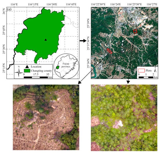
Figure 1.
Location of the study area. (a) Changting County, Longyan City, Fujian Province, China; (b) two sample plots (400 m × 400 m) on Sentinel-2A, representing different levels of vegetation cover (plots A and B); and (c,d) UAV photographs of the two plots.
2.2. Data Collection and Preprocessing
2.2.1. UAV Image Acquisition and Pre-Processing
The UAV data were acquired on 26–27 December 2022 under clear sky conditions. The data collection was conducted using a DJI Phantom 4 quadcopter (DJI Technology Co., Ltd., Shenzhen, China) and its equipped multispectral camera (blue: 450 ± 16 nm, green: 560 ± 16 nm, red: 650 ± 16 nm, red edge: 730 ± 16 nm, and near-infrared: 840 ± 26 nm) for acquisition. The camera has a resolution of million (1600 × 1300) pixels, a 1/2.3′′ CMOS sensor, a lens focal length of 20 mm (35 mm equivalent), and a field of view angle. of 94°. The camera is stabilized by a three-axis gimbal and can acquire multispectral and visible image data simultaneously. After comprehensively evaluating the cost of use, the efficiency of data processing, and ensuring the broad applicability of the study results, we decided to retain only the visible band of the multispectral lens for subsequent processing. Flight route planning was accomplished using a DJI Pro (DJI Technology Co., Ltd., Shenzhen, China), flight altitude was set to be between 90 and 160 m according to the local terrain, and the heading and sidetrack overlap rate was set to 70% to ensure that orthoimages of the slit were acquired. A total of 2442–4486 images were eventually captured. The orthomosaic image generation was conducted using DJI Terra 2.3.3 software (DJI Technology Co., Ltd., Shenzhen, China) to create UAV orthophotos with a spatial resolution of approximately 0.1 cm.
2.2.2. Satellite Image Acquisition and Pre-Processing
Sentinel-2 and Landsat 9 satellite data were selected for landscape-scale FVC mapping in this study. Compared with Landsat 8, Landsat 9 has higher radiometric resolution (14 bits) and can capture more vegetation features in shaded areas. Sentinel-2 has higher revisit frequency (5 days) and spatial resolution (10 m) compared with Landsat series, which can better monitor the dynamic changes of vegetation [7]. All satellite data were pre-processed using the Google Earth Engine (GEE) platform, which provides Sentinel-2 A/B surface reflectance products (calculated by the Sen2Cor processor) and Landsat 9 surface reflectance products (generated by the Land Surface Reflectance Code (LaSRC) generated) [18,19]. To minimize cloud contamination, a multi-temporal compositing approach was employed. Images with less than 10% cloud coverage were acquired from December 2022 to January 2023 (one month before and after the UAV sampling time). The QA60 (Sentinel-2) and QA_PIXEL bitmask bands containing cloud mask information were used to cloudy pixels, and then the raw DN values were converted to surface reflectance according to the officially provided formulas. Finally, the median synthesis approach was employed to produce a complete cloud-free image to minimize the impact of cloud cover as well as cloud shadows on this study [20]. For Sentinel-2A images, blue (B2), green (B3), red (B4), and near-infrared (NIR, (B8)) bands were selected to generate 10 m resolution images, and red edge (B5, B6, and B7) and short-wave infrared (SWIR and (B11 and B12)) bands were selected to generate 20 m resolution images in this study. For Landsat 9 OLI-2 images, the visible-NIR bands (SR2-SR7) were selected to generate 30 m resolution images in this study. The detailed sensor band information is displayed in Table 1.

Table 1.
The band attribute information for Sentinel-2 and Landsat 9.
The pre-processed satellite images were subsequently utilized for feature calculation (Table 2). In the VIs calculation process, we first selected a series of commonly used visible-NIR-based vegetation index VIs, including simple ratio (SR), normalized difference vegetation index (NDVI), enhanced vegetation index (EVI), soil-adjusted vegetation index (SVAI), modified soil-adjusted vegetation index (MSAVI), and kernel normalized difference vegetation index (kNDVI). In addition, based on the unique red-edge and SWIR bands of Sentinel-2A (20 m) and Landsat 9 OLI-2 (30 m), we calculated visible-band red-edge index (VREI), red-edge normalized difference vegetation index (RENDVI), infrared simple ratio (ISR) and the normalized difference water index (NDWI).

Table 2.
The formula of VIs features of Sentinel-2 and Landsat 9 images.
2.3. Methodology
Figure 2 provides a comprehensive overview of the study’s workflow. First, a binary classification map of vegetation and non-vegetation was generated based on drone orthophotos and aggregated into grids of different resolutions (10 m, 20 m, and 30 m) to statistically generate actual FVC. At the same time, the spectral and VIs features from the satellite images were extracted and matched with the corresponding actual FVC to construct a feature-FVC dataset. Subsequently, machine learning modeling and evaluation were performed on the dataset. Finally, the best model was applied to all pixels to achieve regional FVC mapping (predicted FVC).
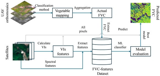
Figure 2.
Flowchart used for deriving the FVC by integrating UAV and multi-scale satellite data.
2.3.1. Binary Classification Based on UAV Images
To obtain accurate vegetation coverage samples, this study compares the performance of three classification methods in distinguishing vegetation from non-vegetation based on UAV RGB images: (1) object-oriented combined with random forests (OBIA-RF); (2) threshold method; and (3) K-means clustering. The OBIA-RF method can make full use of the geometric, spectral, and textural information of high-resolution images to improve the accuracy and efficiency of information extraction with a stronger robustness and generalization ability. It has garnered widespread adoption for the RS-classification process [29]. The threshold method classifies pixels in RS images into different vegetation classes based on specific thresholds of VIs (e.g., NDVI). This method is characterized by its simplicity and directness, eliminating the need for complex mathematical models or computational processes, and is highly adaptable and flexible in setting the thresholds according to the characteristics of specific study areas and vegetation types [30]. The K-means method is an unsupervised classification method that can automatically cluster pixels in RS images according to their spectral features without predefined category labels or training samples. It can process highly dimensional datasets quickly and efficiently.
In the OBIA-RF method, 200 points were first randomly selected in each sample plot, each sample point was assigned a corresponding category label (1 = vegetation, 2 = non-vegetation) by visual interpretation, and the labeled samples were verified and corrected through field survey. Then, the RGB images of each sample site were imported into eCognition software (version 9.5) for multi-scale segmentation, and the optimal segmentation scale was determined using the estimation of scale parameter 2 (ESP2) tool [31]. Finally, based on the optimal segmentation scale, spectral features, VIs features, texture features, and geometric features of the sample objects were extracted, and the RF algorithm was utilized for land cover classification. For VIs, we chose normalized green-red difference index, normalized green-blue difference index (NGBDI), excess green index (EXG), green vegetation index (GVI), and visible-band difference vegetation index (VDVI), which are widely used for vegetation classification. For the thresholding method, due to the absence of NIR bands in RGB images, this study used VDVI [32] instead of NDVI for threshold determination and classification. Optimal VDVI thresholds were determined for each plot (VDVI > 0.6 for plot A, VDVI > 0.7 for plot B) via iterative experimentation and analysis of mean VDVI values derived from optimally segmented vegetation objects. K-means unsupervised classification was implemented in Python using the scikit-learn and rasterio packages.
Precision (Equation (1)) and recall (Equation (2)) were utilized as quantitative metrics to assess the outcomes of the three classification methods [12]. During the model training phase, to mitigate overfitting and ensure model stability, a stratified sampling technique was applied, randomly splitting each class of samples into a training set and a validation set in a 1:1 ratio. The training set was employed for the construction and training of the model, while the validation set was utilized to evaluated the model’s accuracy. Finally, the best classification algorithm was selected for binary classification on the UAV images for subsequent analyses.
In the formula, TP denotes the number of extractions that correctly match the true category, FP denotes the number of cases where the actual situation is background (non-vegetation) but is mistakenly identified as vegetation, and FN denotes the number of cases where vegetation is not correctly detected.
2.3.2. Constructing FVC with VIs and Band Value Datasets
In this study, FVC is defined as the ratio of vegetation pixels identified from UAV classification results to the total number of pixels in a given grid cell. To ensure compatibility across different satellite data resolutions, the UAV image boundaries were utilized to determine the study area of the corresponding satellite images. Grids that are fully aligned with the satellite image pixels are created, excluding the grids that partially overlap with the UAV boundaries. The FVC was calculated by counting the number of vegetation pixels in the corresponding grid using the zonal_stats function in the rasterstats package in Python, and then the band reflectance values and VIs values corresponding to the Sentinel-2 and Landsat 9 images were extracted for each cell center. The data set was constructed by matching the row and column position indexes of the grids, effectively linking FVC values with the corresponding satellite image feature. Eventually, a total of 3000 samples at 10 m resolution, 682 samples at 20 m resolution, and 291 samples at 30 m resolution were collected within the two plots. All of the above steps were processed through Python.
2.3.3. Satellite-Scale FVC Modeling and Accuracy Evaluation
To comprehensively evaluate the potential of different sensors in automatic FVC mapping and explore performance variations among models in the multi-scale FVC inversion, this study used four ML models: K-Nearest Neighbors (KNN), Multilayer Perceptron (MLP), RF, and Extreme Gradient Boosting (XGBoost) to establish the relationships between FVC and features extracted from Sentinel-2A/Landsat 9 OLI-2 images. KNN, a simple and efficient classification method, assigns classes to samples by calculating the distance between a target sample and its k nearest neighbors (e.g., Euclidean distance and Manhattan distance) [33]. MLP, a widely used feed-forward network, makes use of its powerful learning capacity and backpropagation algorithm (BP) to effectively deal with complex nonlinear problems [34]. RF is a decision tree method based on integrated learning, which improves the overall prediction performance by integrating the prediction results of multiple decision trees based on self-help method sampling and random selection of feature space and can effectively deal with multidimensional datasets and avoid overfitting. XGBoost, a highly efficient and stable boosting integrated learning algorithm, builds on the GBDT and RF models. By incorporating the tree model’s complexity as a regular term to the optimization objective and implementing random feature subsampling, XGBoost effectively reduces computational cost, improves efficiency, prevents overfitting, and is suitable for processing large-scale datasets [31].
Optimizing parameters is essential to increasing model accuracy. The four ML models in this study are optimized based on the training dataset using the simulated annealing approach included in the Hyperopt package. The KNN’s primary parameter is n_neighbors. Alpha, activation, and hidden_layer_sizes are the three main MLP parameters. The two most important RF parameters are max-depth and n-estimators. Subsample, learning rate, gamma, colsample_bytree, n_estimators, and max_depth are some of the important XGBoost parameters. The range of values for the four algorithms’ primary parameters is given in Table 3.

Table 3.
Hyperparameters tuning ranges for four machine learning (ML) models.
In this study, the model’s performance was evaluated using three metrics: R2 (Equation (3)), RMSE (Equation (4)), and MAE (Equation (5)) [35]. The smaller the values of MAE and RMSE, coupled with an R2 closer to 1, indicate higher accuracy. In addition, for each scale, the best-performing model was selected and evaluated for uncertainty using the bootstrap resampling technique. Specifically, a total of 100 bootstrap sampling iterations were performed; with each iteration, 70% of the data was randomly selected for model training, and the remaining 30% was utilized for model validation. Additionally, the R2, RMSE, and MAE were calculated for each iteration to assess the overall stability and generalization ability of the models.
In the formula, n denotes the count of samples, denotes the actual FVC, is the predicted FVC, and is the average FVC.
2.3.4. SHapley Additive exPlanation (SHAP) for FVC Model Interpretation
To interpret the model predictions, this study uses the SHAP values to explain the best model at different spatial resolutions. The SHAP method is based on game theory and evaluates feature importance by calculating the average marginal contribution of each feature to the model prediction results [36]. In this study, the contribution of each individual feature to the model predictions is evaluated, and the influence of each feature on the predictions is explained through the generation of summary and dependency graphs using the SHAP approach. The Python shap module is utilized for the computation of SHAP values.
3. Results
3.1. Classification of UAV-Orthomosaic
Based on the confusion matrix, three classification methods (OBIA-RF, threshold, and K-means) were evaluated for their effectiveness in classifying binary vegetation from non-vegetation in areas with varying vegetation cover (Figure 3). The results indicated that the threshold method obtained the highest classification accuracy, with a precision of 0.963 and a recall of 0.929 in plot A (Table 4). OBIA-RF came in second, with precision and recall of 0.897 and 0.929, respectively. K-means performed the worst, with precision and recall of 0.431 and 0.893, respectively. In plot B, the best performance was OBIA-RF, with precision and recall of 0.915 and 0.929. This was followed by thresholding (precision: 0.903, recall: 0.929) and K-means (precision: 0.789, recall: 0.643). Overall, OBIA-RF and threshold frequently produced better results (precision and recall > 0.890) in both plots. The threshold method achieved the best performance, with average precision and recall of 0.933 and 0.929 on both plots, respectively. On the other hand, K-means performed the worst, with average precision and recall of 0.610 and 0.768, respectively.
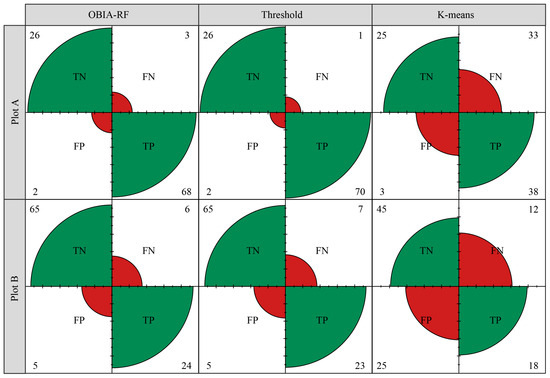
Figure 3.
Confusion matrix of OBIA-RF, thresholding, and K-means.

Table 4.
Accuracy evaluation of vegetation classification results based on different methods.
Figure 4 demonstrates the actual classification output of different methods at the sample plot scale. It is evident that OBIA-RF is better at depicting the distribution area and vegetation border with less fragmentation, which is more in line with the actual conditions of the study region. While the threshold method also performance well, there are several instances of misclassification and omission. For example, shadows cast by canopy overlap in areas with high vegetation cover are often misclassified as vegetation, whereas senescent vegetation is frequently mistaken for non-vegetation in regions with low vegetation cover. When it comes to capturing fine-scale differences in vegetation, especially in areas with low vegetation cover, K-means performs the worst, showing severe plot fragmentation (Plot A). Taking into account both the classification accuracy and the visual evaluation of the output, OBIA-RF was chosen as the approach for the binary classification in UAV images for the subsequent analyses.
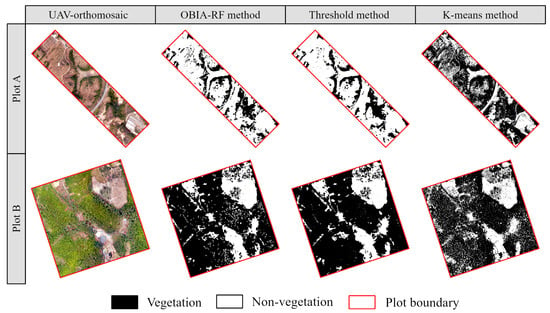
Figure 4.
Comparison of UAV-orthomosaic at plot scale and binary classification results from various machine learning (ML) models.
3.2. FVC Upscaling Based on UAV Classification Results
Figure 5 illustrates the FVC upscaling results for different satellite image resolutions. As the spatial resolution decreases, the range of variation of the image element values shows a convergence trend. This indicates a decrease in variability and an improvement in spatial continuity but at the sacrifice of some information on spatial heterogeneity. The histogram in Figure 6 reveals the dependence of the FVC distribution on the spatial resolution. Overall, the histograms at the three scales showed the same trend, with peak observation density occurring at the two ends of the gradient. These peaks corresponded to the different vegetation cover degrees in sample plots A and B, which coincided with the actual situation. In addition, a decrease in resolution leads to an increase in mixed pixels, causing the distribution to shift toward the center of the scale and resulting in a smoother curve.
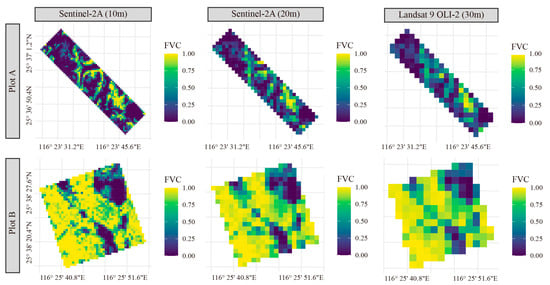
Figure 5.
Binary classification results of UAV-orthomosaics using OBIA-RF methods.
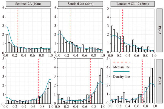
Figure 6.
Binary classification results of UAV-orthomosaic using different classification methods.
3.3. Constructing FVC Estimation Models
This study used four ML models (KNN, MLP, RF, and XGBoost) to estimate the FVC based on Sentinel-2A (10 m and 20 m) and Landsat 9 OLI-2 (30 m) imagery. The results are shown in Figure 7 to evaluate the performance of these models in estimating FVC at different scales. At a 10 m resolution, RF obtained the highest accuracy, with an R2 of 0.827 and an RMSE of 0.169. Compared with KNN, MLP, and XGBoost, RF exhibited improvements in R2 by 0.003, 0.017, and 0.001, respectively. In terms of RMSE, RF showed reductions of 0.001 and 0.008 compared with KNN and MLP, respectively, and performed on par with XGBoost. At a 20 m resolution, the R2 of all four models is greater than 0.900, and the RMSE value is below 0.110. The RF model performs the best, with an R2 of 0.929 and an RMSE of 0.100. Compared to KNN, MLP, and XGBoost, this represented improvements in R2 of 0.003, 0.010, and 0.004, respectively, and reductions in the RMSE of 0.002, 0.007, and 0.003, respectively. At a 30 m resolution, the best-performing model is XGBoost, with R2 and RMSE of 0.847 and 0.145, respectively. Compared to the other models, XGBoost showed improvements in R2 ranging from 0.016 to 0.036 and reductions in RMSE ranging from 0.004 to 0.014. Overall, across the three spatial resolutions, the different ML models achieved R2 values between 0.811 and 0.929 and RMSE values between 0.100 and 0.177. The model based on Sentinel-2A (20 m) had the highest average accuracy, followed by Landsat 9 OLI-2 (30 m) and Sentinel-2A (10 m). From the modeling point of view, tree-based models (RF and XGBoost) demonstrated better adaptability and higher prediction accuracy, with RF and XGBoost methods being selected as the best model in 2 and 1 instances, respectively.
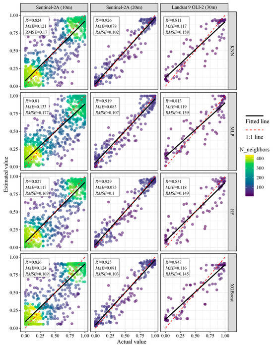
Figure 7.
Scatter plot of FVC measured by UAV and FVC predicted by ML model. N_neighbors represents the number of samples around each sample point.
3.4. Uncertainty of Optimal FVC Model
The best models at different resolutions were further analyzed to explore the uncertainty of the model prediction results. Additionally, SHAP values served as an objective tool to evaluate the impac of various features on the model output. The results showed that the standard deviation of R2 values for the best models at various spatial resolutions was less than 0.05, indicating that the model prediction results are relatively stable (Figure 8). Among them, the Landsat 9 OLI-2 (30 m) model has the largest R2 standard deviation (0.049), while the Sentinel-2A (10 m and 20 m) models had R2 standard deviations of 0.012 and 0.011, respectively.
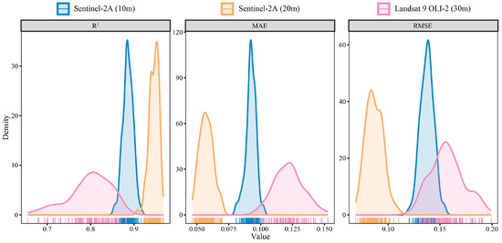
Figure 8.
Evaluation results of 100 bootstrap samples of the best model at different resolutions. The wide distribution of kernel density indicates that there are differences between bootstrap samples.
The summary graph (Figure 9a,c,e) shows the SHAP values of each sample and displays the feature importance according to the average absolute value of SHAP. For the 10 m resolution model, kNDVI has the greatest impact on the model output. The larger kNDVI value corresponded to the larger SHAP value, indicating a positive correlation between kNDVI and FVC. The SR and NDVI features also have significant effects, and they rank second and third in model importance, respectively. The 20 m resolution model exhibited a similar pattern to the 10 m resolution model, with SR having the greatest impact, followed by kNDVI and NDVI. This indicates that the high reflectivity characteristics of vegetation in the NIR play a key role in FVC estimation based on Sentinel-2A images (10 m and 20 m). For the 30 m resolution model, ISR2 has the greatest impact on the model output, and its SHAP value is much higher than other features, followed by NDWI1 and NDVI. The moisture-sensitive VIs rank high, indicating that moisture significantly affects the 30 m resolution model’s estimation of FVC in the study area.
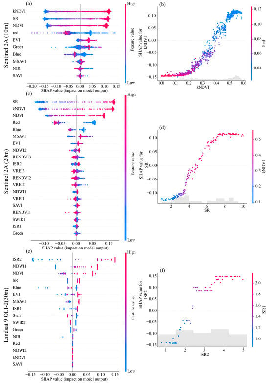
Figure 9.
Shapely additive explanation of the best model at different resolutions. (a,c,e) represent the summary plot of the best model at 10 m, 20 m, and 30 m resolutions, respectively, and (b,d,f) represent the dependency plot of the corresponding data.
The dependency plot in Figure 9b,d,f further illustrates the impact of the most important features of the model and their interactions with other features on model output. For the 10 m resolution model, when kNDVI values were below 0.35, the model estimated lower FVC values (indicated by negative SHAP values). However, as kNDVI increased and red decreased, the model estimates value increased significantly (indicated by positive SHAP values). For the 20 m resolution model, when SR is between 5 and 7, SR and SHAP show a linear relationship as kNDVI increases, which significantly affects the model’s output. In the 30 m resolution model, ISR2 exhibited a similar trend to the 20 m model. When ISR2 is between 2.5 and 3.5, the change in its value affects the model FVC estimate.
Figure 10 shows the satellite-scale FVC and its frequency histogram predicted by the corresponding optimal ML model at each resolution. Despite the different satellite resolutions, the satellite FVC has the same distribution pattern as a whole. For example, the northwest and southeast areas of the study area are the main vegetation coverage areas, which can be identified in all satellite FVC maps. In addition, the similar trends of the histograms indicate that the FVC changes of all satellites are relatively consistent. It is worth noting that the density curve of the higher-resolution satellite had greater fluctuations, indicating that it can better reflect the heterogeneity of the FVC distribution. In summary, the results demonstrate the successful estimation of FVC at different scales using the selected models.
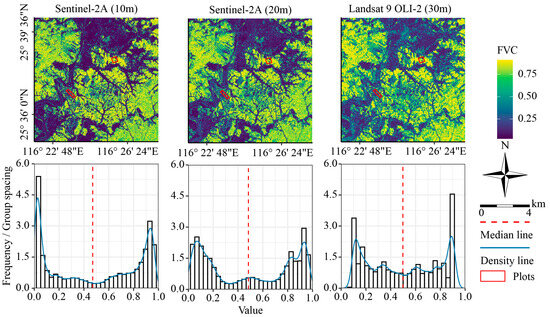
Figure 10.
FVC predictions of the best model at different spatial resolutions across the study area. Plots A and B show the extent of the drone data used to train and validate the model.
4. Discussion
4.1. Mapping Vegetation on the UAV Scale
The key challenge in assessing soil erosion is to find more cost-effective and efficient methods for collecting samples and to ensure that these observations can be reliably correlated with large-scale earth observation data. FVC, as a clear and easily quantifiable indicator, is particularly crucial for assessing the dynamic changes of soil erosion. Although measuring FVC at the plot scale is relatively simple and direct, accurate measurement at the satellite observation scale faces many challenges. However, the introduction of UAV technology provides a new way to invert multi-scale vegetation parameters, making up for the scale difference between field measurement data and satellite observation data and providing scientific and effective technical support for precise monitoring and evaluation of soil erosion.
Accurately extracting vegetation information from UAV images is the key to subsequent FVC calculation and model development. This study compared three commonly used methods: OBIA-RF, the threshold method, and K-means. The findings demonstrate that in both study plots, the OBIA-RF method achieved high classification accuracy and was able to accurately depict the distribution area and boundaries of vegetation. Its capacity to effectively utilize multi-dimensional information, such as space, spectrum, and texture of high-resolution images, is responsible for its exceptional performance [31]. Although the threshold method is simple and quick to apply, it is susceptible to misclassification and omission due to shadows and senescent vegetation. The K-means method has the worst classification effect, with obvious fragmentation of patches, and it is challenging to find subtle variations in areas with little vegetation.
It is noteworthy to mention that although the threshold method achieved the highest accuracy in plot A with low vegetation coverage, it needs to set a suitable threshold according to the specific study area and vegetation type in practical applications. This limits its generalizability. In contrast, the OBIA-RF method can adaptively learn image features and has higher robustness and generalization ability [37], making it more suitable for FVC mapping of large areas with diverse vegetation cover.
4.2. FVC Was Upscaled from UAV to the Sentinel Scale
The scale effect is a crucial issue that necessitates consideration in the process of comprehensively assessing the health status and restoration progress of ecosystems. A deep understanding of the scale effect when the FVC results at the UAV scale are aggregated to the resolution of satellite images is of great significance for more accurately capturing and assessing soil erosion at different spatial scales. This study found that as the spatial resolution decreases, the variability of FVC data decreases, and the continuity of spatial distribution increases, but it is also accompanied by the loss of some spatial heterogeneity information. This phenomenon can be explained by the modifiable area unit problem (MAUP), which states that the spatial analysis results are dependent on the scale and shape of the analysis unit [38]. In this study, the UAV FVC upscaling results of different satellite resolutions show that higher-spatial-resolution data have greater heterogeneity than those with a lower spatial resolution. Histogram analysis further clarified the scale-related effect in MAUP. The output demonstrated that as the resolution decreases, the overall variance of the FVC distribution decreases, and the density curve becomes smoother, which aligns with the output observed by Mao et al. [16]. Peng et al. [39] have shown that MAUP can affect the results of statistical analysis, especially when finer units are aggregated into larger units, the variation of the data decreases, and the model’s explanatory power improves. This, to some extent, explains why the satellite FVC model based on coarser-resolution data (20 m and 30 m) in this study has higher explanatory power and a lower RMSE than the model based on 10 m resolution data.
In addition, this study discovered that the contributions of various spectral features and vegetation indices to FVC estimation models vary. For example, VIs based on red and NIR bands (e.g., SR and NDVI) perform better in models with 10 m and 20 m resolutions, but indices based on short-wave infrared bands perform better at a 30 m resolution. This might be owing to the fact that individual bands have different sensitivities to vegetation and soil information, as well as the proportion of mixed pixels in images with different resolutions is also different, which affects the applicability of different indices [40]. Therefore, in addition to using traditional NDVI, future research needs to focus on these vegetation indices and their combinations.
Our results indicate that the ML model has a better estimation performance in FVC inversion, and the estimation accuracy (R2) of all models is greater than 0.8, similar to the research results found by Yang et al. and Mao et al. [4,16]. This can be attributed to the ability of the ML model to effectively capture the complex nonlinear relationship between FVC and multidimensional data, along with their adaptive adjustment capabilities, resulting in higher prediction accuracy and generalization ability [41]. Furthermore, our research highlights the superior predictive precision and stability of tree-based models (RF and XGBoost), which obtained the best model performance twice and once, respectively. This advantage likely stems from their mechanism of constructing multiple decision trees and merging their prediction outcomes [42,43].
4.3. Limitations and Future Work
Despite demonstrating the effectiveness of our method for FVC estimation, this study also has several weaknesses. First, the UAV images used in this study were limited to a single phase. To increase the precision and timeliness of FVC monitoring, future studies should investigate multi-temporal UAV image-acquisition and processing techniques [44]. Second, more work needs to be performed on the temporal consistency of UAV and satellite data. In particular, synchronized data acquisition between UAV and satellite platforms should be pursued during periods of vigorous vegetation growth to avoid inaccuracies resulting from temporal lag. Secondly, the number of samples in this study is small and concentrated in two research plots. To improve the model’s generalization capability, it is important to expand the sampling scope and optimize the sample size and spatial distribution. Third, this study only used visible light band data for UAV image classification. Future research could investigate combining multi-source RS data, such as multispectral or hyperspectral data [45], to provide richer vegetation information and develop more accurate and robust FVC estimation models. Finally, to increase the precision and effectiveness of FVC estimates, future research should investigate the incorporation of deep learning technology further and take advantage of its potent feature extraction and classification capabilities.
5. Conclusions
This study confirms that combining UAV and multi-scale satellite images and using ML methods to estimate FVC across scales is an effective way to monitor vegetation coverage in soil erosion areas. Among them, UAV observation data can effectively replace traditional ground-based measured data and provide reliable training samples for satellite RS models. This study found that the OBIA-RF method performed best in the binary classification of UAV images and was able to extract high-precision FVC reference data. On this basis, the RF and XGBoost models performed best in FVC estimation of medium and high-resolution satellite images, respectively, indicating that ML methods, especially tree-based models, have great potential in multi-scale FVC inversion. This study also found that there was a substantial relationship between UAV-scale FVC and a variety of medium-resolution satellite image VIs, especially those containing red-edge and NIR bands, and this correlation was more prominent in coarser-resolution data. The findings of this study offer a solid scientific foundation for the formulation of more accurate and efficient vegetation monitoring programs in soil erosion areas in the future while also serving as a valuable reference for other types of ecological environment monitoring.
Author Contributions
Conceptualization, X.C. and K.Y.; methodology, X.C. and X.H.; writing—original draft preparation, X.C., Y.S., and H.Z.; writing—review and editing, X.C., H.Z., Y.S., X.Q., J.C. and M.C.; funding acquisition, H.Z., X.H., and K.Y. All authors have read and agreed to the published version of the manuscript.
Funding
This study was supported by the National Key Research and Development Program of China (2023YFF130440304), the National Natural Science Foundation of China (32371853), the Natural Science Foundation of Fujian Province (2020J05021, 2021J01059), and the Special Fund Project for Science and Technology Innovation of Fujian Agriculture and Forestry University (KFb22033XA).
Data Availability Statement
The data presented in this study are available upon request from the authors.
Conflicts of Interest
The authors declare no conflicts of interest.
References
- Wu, S.; Deng, L.; Zhai, J.; Lu, Z.; Wu, Y.; Chen, Y.; Guo, L.; Gao, H. Approach for Monitoring Spatiotemporal Changes in Fractional Vegetation Cover Through Unmanned Aerial System-Guided-Satellite Survey: A Case Study in Mining Area. IEEE J. Sel. Top. Appl. Earth Obs. Remote Sens. 2023, 16, 5502–5513. [Google Scholar] [CrossRef]
- Wang, K.; Zhou, J.; Tan, M.L.; Lu, P.; Xue, Z.; Liu, M.; Wang, X. Impacts of Vegetation Restoration on Soil Erosion in the Yellow River Basin, China. Catena 2024, 234, 107547. [Google Scholar] [CrossRef]
- Yan, K.; Gao, S.; Chi, H.; Qi, J.; Song, W.; Tong, Y.; Mu, X.; Yan, G. Evaluation of the Vegetation-Index-Based Dimidiate Pixel Model for Fractional Vegetation Cover Estimation. IEEE Trans. Geosci. Remote Sens. 2022, 60, 1–14. [Google Scholar] [CrossRef]
- Yang, S.; Li, S.; Zhang, B.; Yu, R.; Li, C.; Hu, J.; Liu, S.; Cheng, E.; Lou, Z.; Peng, D. Accurate Estimation of Fractional Vegetation Cover for Winter Wheat by Integrated Unmanned Aerial Systems and Satellite Images. Front. Plant Sci. 2023, 14, 1220137. [Google Scholar] [CrossRef]
- Zhang, Z. Stand Density Estimation Based on Fractional Vegetation Coverage from Sentinel-2 Satellite Imagery. Int. J. Appl. Earth Obs. Geoinf. 2022, 108, 102760. [Google Scholar] [CrossRef]
- Bian, J.; Li, A.; Zhang, Z.; Zhao, W.; Lei, G.; Yin, G.; Jin, H.; Tan, J.; Huang, C. Monitoring Fractional Green Vegetation Cover Dynamics over a Seasonally Inundated Alpine Wetland Using Dense Time Series HJ-1A/B Constellation Images and an Adaptive Endmember Selection LSMM Model. Remote Sens. Environ. 2017, 197, 98–114. [Google Scholar] [CrossRef]
- Riihimäki, H.; Luoto, M.; Heiskanen, J. Estimating Fractional Cover of Tundra Vegetation at Multiple Scales Using Unmanned Aerial Systems and Optical Satellite Data. Remote Sens. Environ. 2019, 224, 119–132. [Google Scholar] [CrossRef]
- Melville, B.; Fisher, A.; Lucieer, A. Ultra-High Spatial Resolution Fractional Vegetation Cover from Unmanned Aerial Multispectral Imagery. Int. J. Appl. Earth Obs. Geoinf. 2019, 78, 14–24. [Google Scholar] [CrossRef]
- Maurya, A.K.; Nadeem, M.; Singh, D.; Singh, K.P.; Rajput, N.S. Critical Analysis of Machine Learning Approaches for Vegetation Fractional Cover Estimation Using Drone and Sentinel-2 Data. In Proceedings of the 2021 IEEE International Geoscience and Remote Sensing Symposium IGARSS, Brussels, Belgium, 11–16 July 2021; pp. 343–346. [Google Scholar]
- Niu, Y.; Han, W.; Zhang, H.; Zhang, L.; Chen, H. Estimating Fractional Vegetation Cover of Maize under Water Stress from UAV Multispectral Imagery Using Machine Learning Algorithms. Comput. Electron. Agric. 2021, 189, 106414. [Google Scholar] [CrossRef]
- Wang, Q.; Moreno-Martínez, Á.; Muñoz-Marí, J.; Campos-Taberner, M.; Camps-Valls, G. Estimation of Vegetation Traits with Kernel NDVI. ISPRS J. Photogramm. Remote Sens. 2023, 195, 408–417. [Google Scholar] [CrossRef]
- Ye, Z.; Yang, K.; Lin, Y.; Guo, S.; Sun, Y.; Chen, X.; Lai, R.; Zhang, H. A Comparison between Pixel-Based Deep Learning and Object-Based Image Analysis (OBIA) for Individual Detection of Cabbage Plants Based on UAV Visible-Light Images. Comput. Electron. Agric. 2023, 209, 107822. [Google Scholar] [CrossRef]
- Kattenborn, T.; Lopatin, J.; Förster, M.; Braun, A.C.; Fassnacht, F.E. UAV Data as Alternative to Field Sampling to Map Woody Invasive Species Based on Combined Sentinel-1 and Sentinel-2 Data. Remote Sens. Environ. 2019, 227, 61–73. [Google Scholar] [CrossRef]
- Gränzig, T.; Fassnacht, F.E.; Kleinschmit, B.; Förster, M. Mapping the Fractional Coverage of the Invasive Shrub Ulex Europaeus with Multi-Temporal Sentinel-2 Imagery Utilizing UAV Orthoimages and a New Spatial Optimization Approach. Int. J. Appl. Earth Obs. Geoinf. 2021, 96, 102281. [Google Scholar] [CrossRef]
- Lu, L.; Luo, J.; Xin, Y.; Duan, H.; Sun, Z.; Qiu, Y.; Xiao, Q. How Can UAV Contribute in Satellite-Based Phragmites Australis Aboveground Biomass Estimating? Int. J. Appl. Earth Obs. Geoinf. 2022, 114, 103024. [Google Scholar] [CrossRef]
- Mao, P.; Ding, J.; Jiang, B.; Qin, L.; Qiu, G.Y. How Can UAV Bridge the Gap between Ground and Satellite Observations for Quantifying the Biomass of Desert Shrub Community? ISPRS J. Photogramm. Remote Sens. 2022, 192, 361–376. [Google Scholar] [CrossRef]
- Lin, C.; Zhou, S.-L.; Wu, S.-H.; Liao, F.-Q. Relationships Between Intensity Gradation and Evolution of Soil Erosion: A Case Study of Changting in Fujian Province, China. Pedosphere 2012, 22, 243–253. [Google Scholar] [CrossRef]
- Liu, L.; Xiao, X.; Qin, Y.; Wang, J.; Xu, X.; Hu, Y.; Qiao, Z. Mapping Cropping Intensity in China Using Time Series Landsat and Sentinel-2 Images and Google Earth Engine. Remote Sens. Environ. 2020, 239, 111624. [Google Scholar] [CrossRef]
- Tamiminia, H.; Salehi, B.; Mahdianpari, M.; Quackenbush, L.; Adeli, S.; Brisco, B. Google Earth Engine for geo-big data applications: A meta-analysis and systematic review. ISPRS J. Photogramm. Remote Sens. 2020, 164, 152–170. [Google Scholar] [CrossRef]
- Chen, A.; Xu, C.; Zhang, M.; Guo, J.; Xing, X.; Yang, D.; Xu, B.; Yang, X. Cross-Scale Mapping of above-Ground Biomass and Shrub Dominance by Integrating UAV and Satellite Data in Temperate Grassland. Remote Sens. Environ. 2024, 304, 114024. [Google Scholar] [CrossRef]
- Birth, G.S.; McVey, G.R. Measuring the Color of Growing Turf with a Reflectance Spectrophotometer1. Agron. J. 1968, 60, 640–643. [Google Scholar] [CrossRef]
- Huete, A.; Didan, K.; Miura, T.; Rodriguez, E.P.; Gao, X.; Ferreira, L.G. Overview of the Radiometric and Biophysical Performance of the MODIS Vegetation Indices. Remote Sens. Environ. 2002, 83, 195–213. [Google Scholar] [CrossRef]
- Zeng, Y.; Hao, D.; Huete, A.; Dechant, B.; Berry, J.; Chen, J.M.; Joiner, J.; Frankenberg, C.; Bond-Lamberty, B.; Ryu, Y.; et al. Optical Vegetation Indices for Monitoring Terrestrial Ecosystems Globally. Nat. Rev. Earth Environ. 2022, 3, 477–493. [Google Scholar] [CrossRef]
- Qi, J.; Chehbouni, A.; Huete, A.R.; Kerr, Y.H.; Sorooshian, S. A Modified Soil Adjusted Vegetation Index. Remote Sens. Environ. 1994, 48, 119–126. [Google Scholar] [CrossRef]
- Gitelson, A.; Merzlyak, M.N. Quantitative Estimation of Chlorophyll-a Using Reflectance Spectra: Experiments with Autumn Chestnut and Maple Leaves. J. Photochem. Photobiol. B Biol. 1994, 22, 247–252. [Google Scholar] [CrossRef]
- Vogelmann, J.E.; ROCK, B.N.; MOSS, D.M. Red Edge Spectral Measurements from Sugar Maple Leaves. Int. J. Remote Sens. 1993, 14, 1563–1575. [Google Scholar] [CrossRef]
- Fernandes, R.; Butson, C.; Leblanc, S.; Latifovic, R. Landsat-5 TM and Landsat-7 ETM+ Based Accuracy Assessment of Leaf Area Index Products for Canada Derived from SPOT-4 VEGETATION Data. Can. J. Remote Sens. 2003, 29, 241–258. [Google Scholar] [CrossRef]
- Gao, B. NDWI—A Normalized Difference Water Index for Remote Sensing of Vegetation Liquid Water from Space. Remote Sens. Environ. 1996, 58, 257–266. [Google Scholar] [CrossRef]
- Guo, Q.; Zhang, J.; Guo, S.; Ye, Z.; Deng, H.; Hou, X.; Zhang, H. Urban Tree Classification Based on Object-Oriented Approach and Random Forest Algorithm Using Unmanned Aerial Vehicle (UAV) Multispectral Imagery. Remote Sens. 2022, 14, 3885. [Google Scholar] [CrossRef]
- Li, L.; Mu, X.; Jiang, H.; Chianucci, F.; Hu, R.; Song, W.; Qi, J.; Liu, S.; Zhou, J.; Chen, L.; et al. Review of Ground and Aerial Methods for Vegetation Cover Fraction (fCover) and Related Quantities Estimation: Definitions, Advances, Challenges, and Future Perspectives. ISPRS J. Photogramm. Remote Sens. 2023, 199, 133–156. [Google Scholar] [CrossRef]
- Fu, B.; Zuo, P.; Liu, M.; Lan, G.; He, H.; Lao, Z.; Zhang, Y.; Fan, D.; Gao, E. Classifying Vegetation Communities Karst Wetland Synergistic Use of Image Fusion and Object-Based Machine Learning Algorithm with Jilin-1 and UAV Multispectral Images. Ecol. Indic. 2022, 140, 108989. [Google Scholar] [CrossRef]
- Zhou, H.; Fu, L.; Sharma, R.P.; Lei, Y.; Guo, J. A Hybrid Approach of Combining Random Forest with Texture Analysis and VDVI for Desert Vegetation Mapping Based on UAV RGB Data. Remote Sens. 2021, 13, 1891. [Google Scholar] [CrossRef]
- Rehman, T.U.; Mahmud, M.S.; Chang, Y.K.; Jin, J.; Shin, J. Current and Future Applications of Statistical Machine Learning Algorithms for Agricultural Machine Vision Systems. Comput. Electron. Agric. 2019, 156, 585–605. [Google Scholar] [CrossRef]
- Li, S.; Jiang, B.; Liang, S.; Peng, J.; Liang, H.; Han, J.; Yin, X.; Yao, Y.; Zhang, X.; Cheng, J.; et al. Evaluation of Nine Machine Learning Methods for Estimating Daily Land Surface Radiation Budget from MODIS Satellite Data. Int. J. Digit. Earth 2022, 15, 1784–1816. [Google Scholar] [CrossRef]
- Du, Z.; Sun, X.; Zheng, S.; Wang, S.; Wu, L.; An, Y.; Luo, Y. Optimal biochar selection for cadmium pollution remediation in Chinese agricultural soils via optimized machine learning. J. Hazard. Mater. 2024, 476, 135065. [Google Scholar] [CrossRef] [PubMed]
- Minh, D.; Wang, H.X.; Li, Y.F.; Nguyen, T.N. Explainable Artificial Intelligence: A Comprehensive Review. Artif. Intell. Rev. 2022, 55, 3503–3568. [Google Scholar] [CrossRef]
- Fu, B.; Liu, M.; He, H.; Lan, F.; He, X.; Liu, L.; Huang, L.; Fan, D.; Zhao, M.; Jia, Z. Comparison of Optimized Object-Based RF-DT Algorithm and SegNet Algorithm for Classifying Karst Wetland Vegetation Communities Using Ultra-High Spatial Resolution UAV Data. Int. J. Appl. Earth Obs. Geoinf. 2021, 104, 102553. [Google Scholar] [CrossRef]
- Deng, H.; Liu, K.; Feng, J. Understanding the Impact of Modifiable Areal Unit Problem on Urban Vitality and Its Built Environment Factors. Geo-Spat. Inf. Sci. 2024, 1–17. [Google Scholar] [CrossRef]
- Peng, D.; Wang, Y.; Xian, G.; Huete, A.R.; Huang, W.; Shen, M.; Wang, F.; Yu, L.; Liu, L.; Xie, Q.; et al. Investigation of Land Surface Phenology Detections in Shrublands Using Multiple Scale Satellite Data. Remote Sens. Environ. 2021, 252, 112133. [Google Scholar] [CrossRef]
- Gonsamo, A.; Chen, J.M. Spectral Response Function Comparability Among 21 Satellite Sensors for Vegetation Monitoring. IEEE Trans. Geosci. Remote Sens. 2013, 51, 1319–1335. [Google Scholar] [CrossRef]
- Singha, C. Integrating Geospatial, Remote Sensing, and Machine Learning for Climate-Induced Forest Fire Susceptibility Mapping in Similipal Tiger Reserve, India. For. Ecol. Manag. 2024, 555, 121729. [Google Scholar] [CrossRef]
- Zhao, C.; Jia, M.; Wang, Z.; Mao, D.; Wang, Y. Identifying Mangroves through Knowledge Extracted from Trained Random Forest Models: An Interpretable Mangrove Mapping Approach (IMMA). ISPRS J. Photogramm. Remote Sens. 2023, 201, 209–225. [Google Scholar] [CrossRef]
- Alerskans, E.; Zinck, A.-S.P.; Nielsen-Englyst, P.; Høyer, J.L. Exploring Machine Learning Techniques to Retrieve Sea Surface Temperatures from Passive Microwave Measurements. Remote Sens. Environ. 2022, 281, 113220. [Google Scholar] [CrossRef]
- Wei, L.; Yang, H.; Niu, Y.; Zhang, Y.; Xu, L.; Chai, X. Wheat Biomass, Yield, and Straw-Grain Ratio Estimation from Multi-Temporal UAV-Based RGB and Multispectral Images. Biosyst. Eng. 2023, 234, 187–205. [Google Scholar] [CrossRef]
- Putkiranta, P.; Räsänen, A.; Korpelainen, P.; Erlandsson, R.; Kolari, T.H.M.; Pang, Y.; Villoslada, M.; Wolff, F.; Kumpula, T.; Virtanen, T. The Value of Hyperspectral UAV Imagery in Characterizing Tundra Vegetation. Remote Sens. Environ. 2024, 308, 114175. [Google Scholar] [CrossRef]
Disclaimer/Publisher’s Note: The statements, opinions and data contained in all publications are solely those of the individual author(s) and contributor(s) and not of MDPI and/or the editor(s). MDPI and/or the editor(s) disclaim responsibility for any injury to people or property resulting from any ideas, methods, instructions or products referred to in the content. |
© 2024 by the authors. Licensee MDPI, Basel, Switzerland. This article is an open access article distributed under the terms and conditions of the Creative Commons Attribution (CC BY) license (https://creativecommons.org/licenses/by/4.0/).