Abstract
Traditional Newmark models estimate earthquake-induced landslide hazards by calculating permanent displacements exceeding the critical acceleration, which is determined from static factors of safety and hillslope geometries. However, these studies typically predict the potential landslide mass only for the source area, rather than the entire landslide zone, which includes both the source and sliding/depositional areas. In this study, we present a modified Newmark Runout model that incorporates sliding and depositional areas to improve the estimation of landslide chain risks. This model defines the landslide runout as the direction from the source area to the nearest river channel within the same slope unit, simulating natural landslide behavior under gravitational effects, which enables the prediction of the entire landslide zone. We applied the model to a subset of the Minjiang Catchment affected by the 1933 MW 7.3 Diexi Earthquake in China to assess long-term landslide chain risks. The results indicate that the predicted total landslide zone closely matches that of the Xinmo Landslide that occurred on 24 June 2017, despite some uncertainties in the sliding direction caused by the old landslide along the sliding path. Distance-weighted kernel density analysis was used to reduce the prediction uncertainties. The hazard levels of the buildings and roads were determined by the distance to the nearest entire landslide zone, thereby assessing the landslide risk. The landslide dam risks were estimated using the kernel density module for channels blocked by the predicted landslides, modeling intersections of the total landslide zone and the channels. High-risk landslide dam zones spatially correspond to the locations of the knickpoints primarily induced by landslide dams, validating the model’s accuracy. These analyses demonstrate the effectiveness of the presented model for Newmark-based landslide risk estimations, with implications for geohazard chain risk assessments, risk mitigation, and land use planning and management.
1. Introduction
Large earthquakes initiate chains of surface processes that last much longer than the brief moments of strong shaking [1]. Especially in tectonically active mountainous areas, the regional landslide hazards tend to be devastating because of rapid tectonic uplift and frequent seismic activities [2,3]. These factors cause large amounts of landslide mass wasting and create numerous potentially unstable hillslopes that can be triggered by external factors, such as seismic activities, rainfall events, and gravitational effects [4,5,6]. These landslides can destroy infrastructures and block channels, posing an additional long-term threat to populations following an earthquake [7,8]. It is crucial to assess the risks to infrastructures and the potential for landslide dams posed by these unstable hillslopes to enhance regional landslide hazard prevention and prediction [9].
Seismically induced landslide hazards are traditionally assessed based on GIS platforms [10,11,12]. Most GIS-based landslide hazard assessments adopt the Newmark model to predict seismically induced landslide hazards. By simulating the landslide process as a rigid block sliding on an assumed infinitely long plane, the traditional Newmark model directly predicts potential landslides by computing the critical acceleration (AC) of a slope [13,14]. Landslides initially fail from hillslopes and subsequently travel along pathways until they exhaust their gravitational potential energy and accumulate in low-relief terrains [15]. Consequently, the prediction of the entire landslide zone should include not only the landslide source area but also the sliding/depositional areas. However, the traditional Newmark model often simulates potential landslide areas as source areas instead of entire landslide zones, which include both the source and sliding/depositional areas.
Currently, few models for seismically induced landslide susceptibility integrate both slope stability and runout [10,16]. The Rockfall Analyst model is a recent method commonly used for landslide runout simulations, employing a parabolic equation to model landslides as rockfalls [17]. However, it simulates landslides as pixel-based failure cells rather than unified shapes formed by nearby failure cells, making it challenging to capture realistic landslide geometries. Additionally, due to the lack of an empirical relationship between landslide runout distances and volumes, rockfall-based simulations potentially underestimate landslide runout distances, as runout generally increases with landslide area or volume. Another limitation is that these numerical simulation tools are often costly and time consuming, making them impractical for rapid regional landslide susceptibility assessments and less accessible to regular users. To address these challenges, we model each landslide as a collection of nearby failure cells and define the runout direction as the path from the source area to the nearest river channel, using GIS and the R platform. However, this approach may result in incorrect sliding directions. For example, landslides crossing ridgelines may produce only a single sliding route instead of multiple routes along different hillslope aspects bounded by ridgelines. Slope units, which are fundamental geomorphic units derived from slope gradients and aspects, are commonly used in geological hazard analysis [18,19]. These slope units are divided by ridgelines, river valleys, and hillslopes [20], allowing for the unified landslide shape to be divided into smaller shapes constrained by topographic boundaries, which helps to reduce errors in determining sliding directions. As a result, the Newmark-based landslide runout direction is modeled as the path from the potential source area to the nearest channel within the same slope unit, simulating natural landsliding processes influenced by gravitational forces.
This study utilizes the GRASSGIS-platform-based r.slopeunits V1.0 module to extract slope units from the Diexi Catchment in southwestern China. Slope units, geometric modeling, and empirical landslide runout distances are integrated to develop an improved Newmark model called Newmark Runout, which predicts the entire landslide zone, including both the source and sliding/depositional areas. We applied this model to the Diexi Catchment, which was severely affected by the 1933 MW 7.3 Diexi Earthquake, to assess long-term landslide chain risks. The hazard levels of the buildings and roads were determined by the distance to the nearest total landslide zone in assessing the landslide risk. The landslide dam risks were estimated using the kernel density module for channels blocked by the predicted landslides, modeling intersections of the total landslide zone and the channels. Our study offers an effective method for Newmark-based landslide risk estimations, with implications for geohazard chain risk assessments, risk mitigation, and land use planning and management.
2. Materials and Methods
2.1. Study Area
2.1.1. Geomorphological Setting
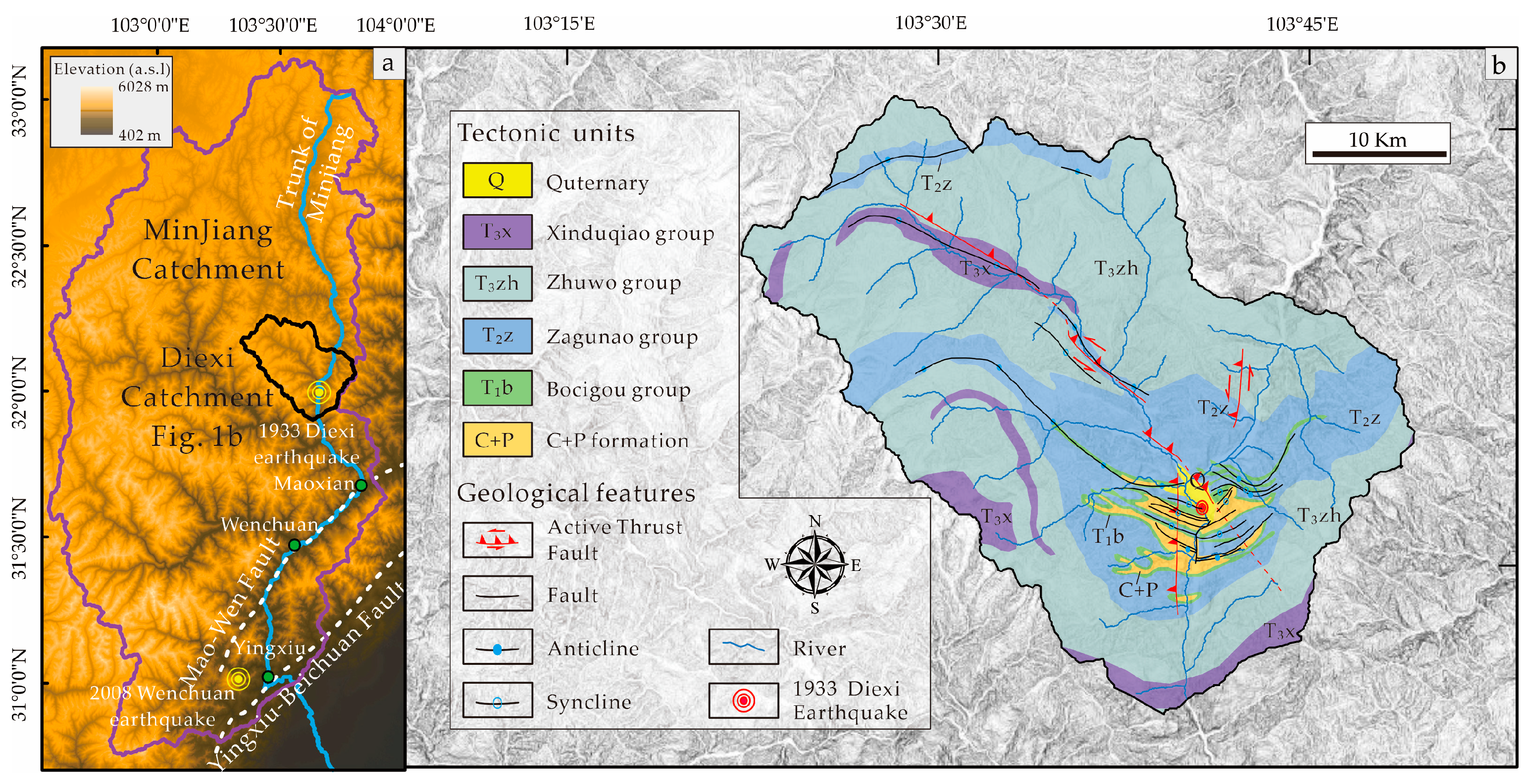
Within the combined region of the Songpan–Ganzi Fold Belt and the Longmenshan Fault Zone, the Diexi Catchment is situated in the boundary shift between the Tibet Plateau and the Sichuan Basin [21]. The Qinghai–Tibet Plateau abruptly changes to the Sichuan Basin, forming the transitional topography of the Longmenshan Fault Zone, which is made up of three NE-striking faults: the Guanxian–Anxian Fault, the Yingxiu–Beichuan Fault, and the Mao–Wen Fault [22] (Figure 1a). Neotectonic activities and regional uplift created one of the major continental escarpments in the world, which has been extensively carved by rivers, notably the main stem of the Minjiang River located in Aba Prefecture, China [23]. The fluvial incision rate of the lower reaches of the Minjiang River is five times higher than the uplift rate of the Longmen Shan, which is still occurring at a pace of 0.3–0.4 mm/year [24]. Since the Pliocene (about 1.58–3.48 Ma), the fluvial incision rate upstream of the Minjiang River has reached 1.19 mm/year, creating a deep canyon beyond a local relief of 2000 m [24]. The Diexi Catchment is located upstream of the Minjiang River, where the river valley has a unique geometric structure, with a vast valley at the top and a gorge at the bottom. This topography segment shows a transition zone between the gorge and the wide valley from 2300 to 2500 m a.s.l. [25].

Figure 1.
Geomorphic and geological settings of the Diexi Catchment [25]. (a) Topographic map of the Diexi Catchment (black boundary) within the Minjiang Catchment (purple boundary); (b) geological map of the Diexi Catchment. Detailed description of lithological units is shown in Figure 2.
2.1.2. Geological Setting
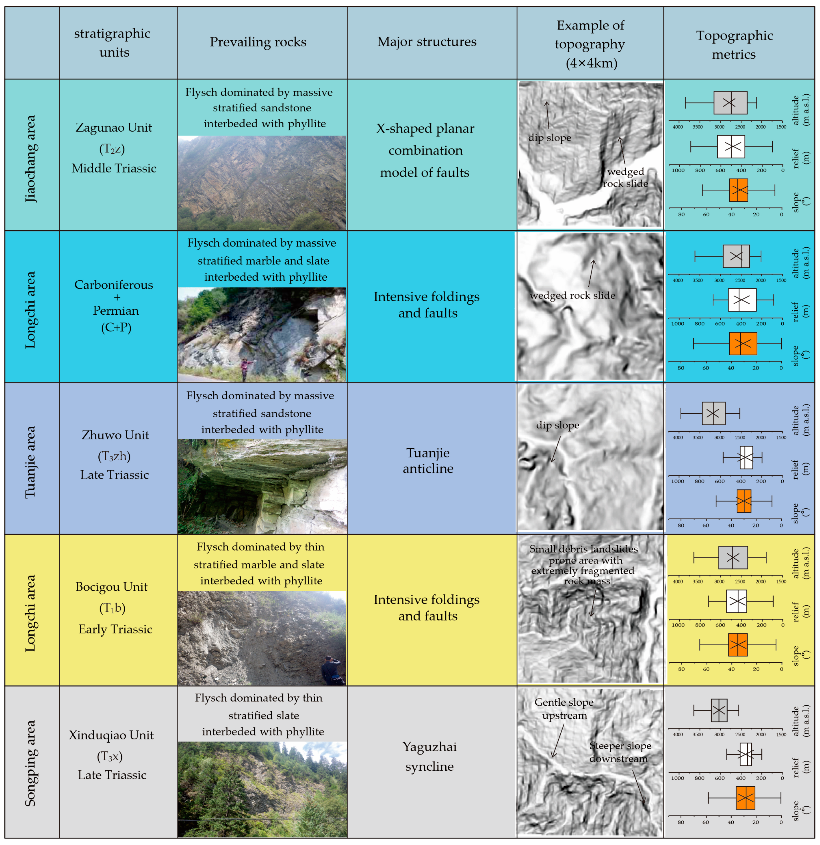
The Jiaochang arc-shaped tectonic zone comprises several thrust faults and immensely overturned folds in the Diexi Catchment [26]. An X-shaped formation results from the intersection of the NS-striking Minjiang Fault and the NE-striking Songpinggou Fault [27]. The interbedded flysch formations are well exposed in the study area. A thick-bedded flysch with a preponderance of sandstones and marbles comprises the Zagunao Unit, the Carboniferous Unit, and the Permian Unit. A flysch, with moderate layers, comprises the Zhuwo Unit. The Xinduqiao Unit and Bocigou Unit are composed of several layers of thin-bedded slates and sandstones with phyllites and mudstones interspersed between them [28]. The detailed characteristics of the stratigraphic units are shown in Figure 1b and Figure 2.

Figure 2.
Description of lithological units in the study area. The colors in the figure correspond to the strata in Figure 1.
Figure 2.
Description of lithological units in the study area. The colors in the figure correspond to the strata in Figure 1.
2.1.3. Historical Earthquakes
Three large historical earthquakes have occurred within 300 km of the Diexi Catchment: the 1933 MW 7.3 Diexi Earthquake (the epicenter was located in the catchment), the 1976 MW 6.9 Songpan–Pingwu Earthquake (32.752°N, 104.157°E), and the 2008 MW 7.9 Wenchuan Earthquake (31.002°N, 103.322°E). The Wenchuan Earthquake had a maximum Modified Mercalli intensity of VII in the Songping area near its epicenter [29]. The highest Modified Mercalli intensity in the study area, located 118 km from the epicenter, was VI [30]. The epicenter of the Songpan–Pingwu Earthquake was situated around 84 km from the study area. The Songpinggou Fault is the seismogenic fault responsible for the Diexi Earthquake, which had a maximum Modified Mercalli intensity of X and was classified as a strike–slip earthquake [31]. The Songping Valley, a Minjiang River branch valley, hosts its epicentral region (Figure 1).
2.2. Methods
The Newmark Runout model was developed by incorporating slope units and sliding areas to estimate the seismic landslide risk in the Diexi Catchment. The detailed steps are as follows: (1) Modified Newmark analysis: The modified Newmark analysis was performed by incorporating topographic site effects, earthquake-induced strength reductions, and structural effects, predicting the potential landslide source areas using the outcome of the CPSHA as regional PGA input; (2) Slope unit extraction: The slope units of the Diexi Catchment were automatically extracted with the GRASS GIS platform; (3) Landslide runout modeling: The landslide runout was derived by modeling the landslide runout from the source area to the nearest channel within the same slope unit based on the fundamental principles of computer graphics and geomorphic processes; and (4) Risk estimation: Remote sensing, landslide interpretation, and the GIS-based kernel density module were applied to estimate and verify infrastructural and landslide dam risks.
2.2.1. Review of the Newmark Model
The spatial analysis of the landslide distribution relies on the Newmark model [13]. In earthquake-induced landslide research, the traditional Newmark model is a rapid and effective method commonly used in regional landslide hazard prediction [32,33]. The Newmark model calculates the slope stability by inputting the peak ground acceleration, slope gradient, and hillslope strength parameters [10].
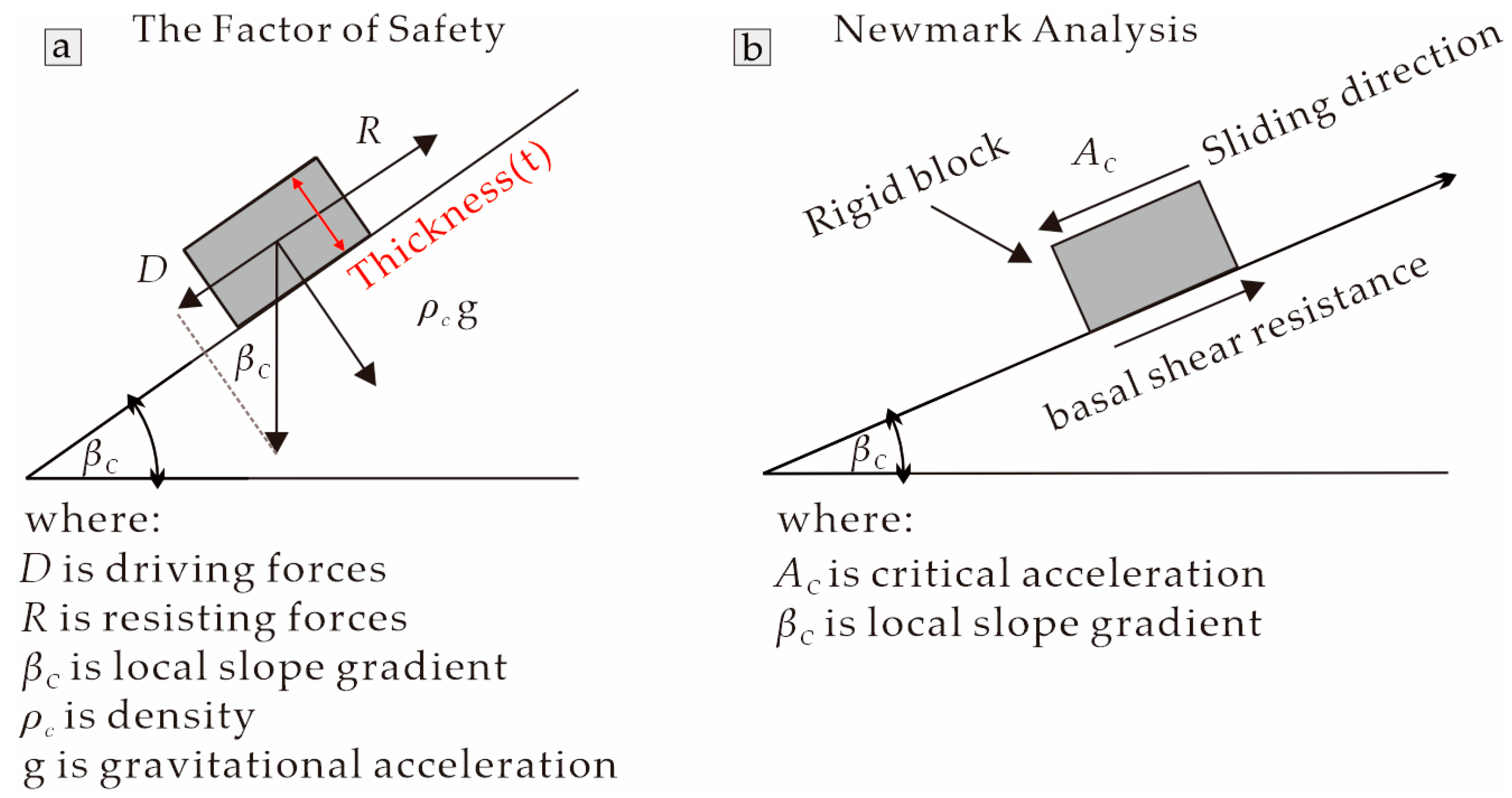
The Newmark model first calculates the factor of the safety/pseudo-static slope stability by defining the factor safety (FS), which describes the ratio of the shear resistance to the shear stress for downslope movements (Figure 3a). The safety factor (FS) is calculated as follows:
where the hillslope strength parameters refer to the internal frictional angle (φ) and cohesion (c), t is an assumed slope failure depth, γ is the bulk density of the hillslope, m is the ratio of the saturated thickness to the total slope failure depth, and βC is the slope gradient. The third term comprises optional parameters related to the pore–water pressure generally formed by groundwater and rainfall. Considering strong earthquakes rarely occur during rainfall events, we assume m = 0 for our analyses.
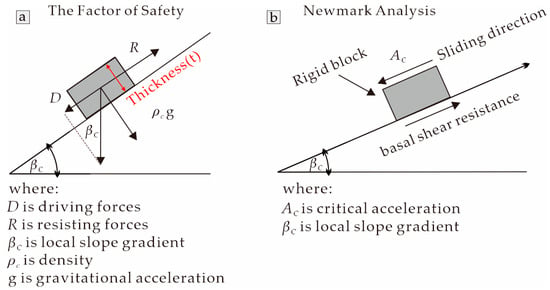
Figure 3.
Sketch illustration of sliding block model. (a) Force balance utilized in Equation (1) is for a block that is sitting on an inclined plane; (b) schematic illustration of the Newmark model.
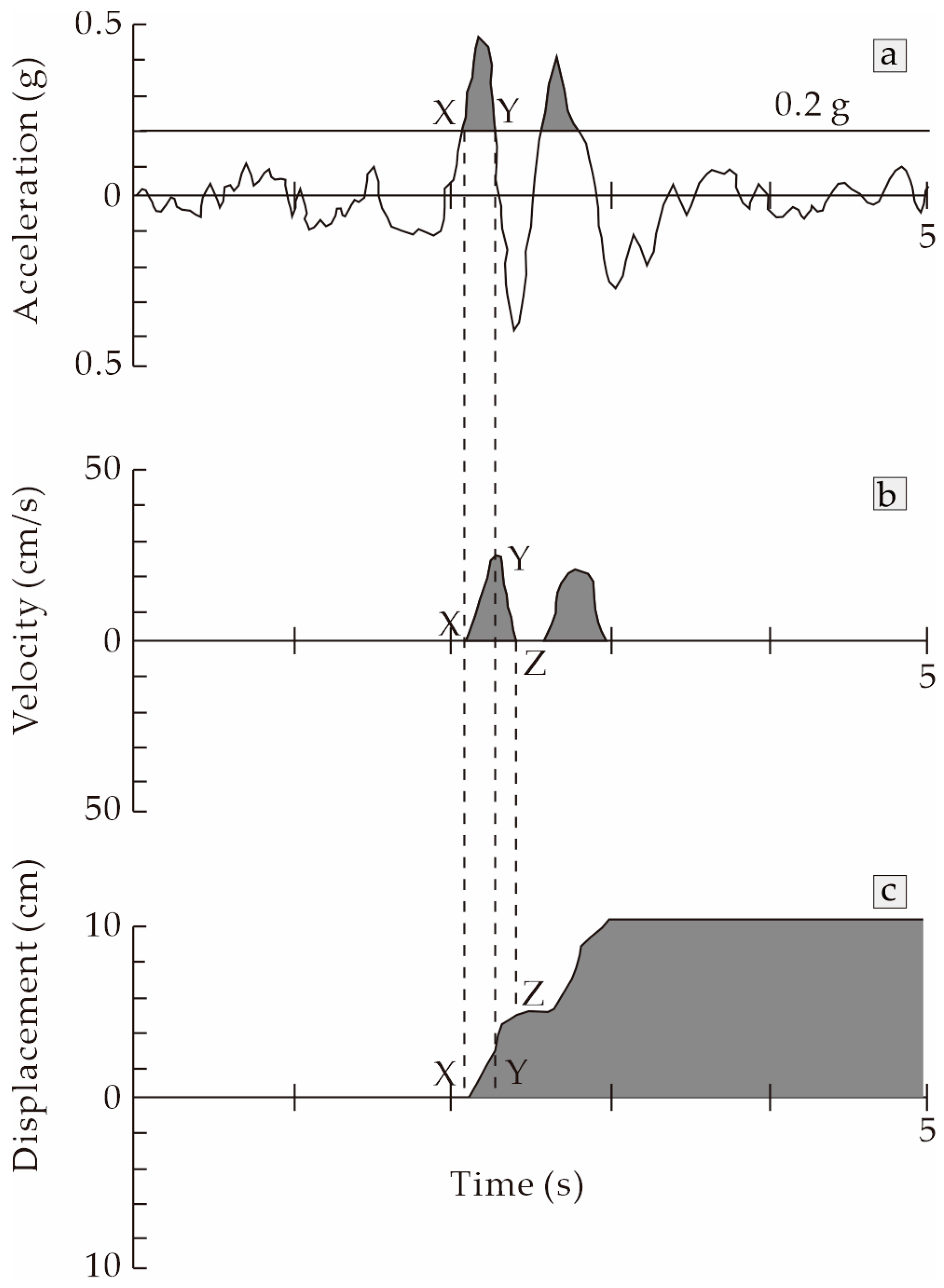
The Newmark analysis models a potential landslide as a sliding block on an inclined plane, with a critical acceleration (AC) necessary to initiate slope failure (Figure 3b). The block displacement along the slope is calculated considering the critical acceleration necessary to initiate the displacement. The critical acceleration (AC) is calculated as follows:
where g is the gravitational acceleration. The permanent displacement (Newmark displacement, DN) can be derived by calculating the double integral of AC, which is generally measured using a real-time seismic accelerometer (Figure 4).
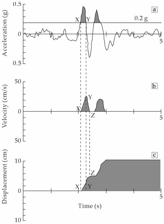
Figure 4.
Double integral to calculate Newmark’s permanent displacement based on real-time spectral acceleration. (a) Real-time seismic spectral acceleration; (b) velocity versus time; (c) permanent displacement versus time. Points X, Y, and Z are critical state beyond critical acceleration; Earthquake acceleration-time history with critical acceleration (solid line) of 0.20 g superimposed.
However, obtaining the real-time spectral acceleration is challenging because of the lack of seismic accelerometers in tectonically active mountainous areas. To address this issue, Jibson et al. [32] proposed an empirical function relating displacement to the ratio between AC and PGA based on a large number of recorded earthquake events.
When using Newmark models, hillslopes with FS values below 1.0 often lead to computational errors because AC becomes negative. Therefore, some previous studies increased FS values from below 1.0 to 1.01 to avoid negative AC values. Although this approach addresses computational errors, it contradicts the Newmark analysis by showing AC increasing with slope gradient. Therefore, according to prior studies [34,35], the ratio of AC to PGA is used and naturally divided on the GIS platform for landslide hazard estimations.
2.2.2. Description of the Newmark Model’s Inputs
We used the ALOS DEM (~12.5 m resolution) derived from the NASA website (https://search.earthdata.nasa.gov accessed on 21 September 2024) to generate slope gradients with the D8 algorithm based on the ArcGIS Raster Surface function, as shown in Figure 5a. The lithological units were digitized from the 1:200,000 scale Maowen geological map and the 1:200,000 scale Songpan geological map, as shown in Figure 5b. Dreyfus et al. [33] argue that optimizing hillslope strength and seismic movement parameters effectively improves the simplified Newmark model. The geotechnical characterization of hillslope materials poses significant challenges for physically based models, primarily because of the limited availability of high-quality shear strength data in many regions. Moreover, the inherent spatial variability of physical properties within lithological groups complicates the accurate assessment of regional rock mass properties [36]. As a result, assigning relative rock mass strengths is often more feasible than determining absolute strength values.
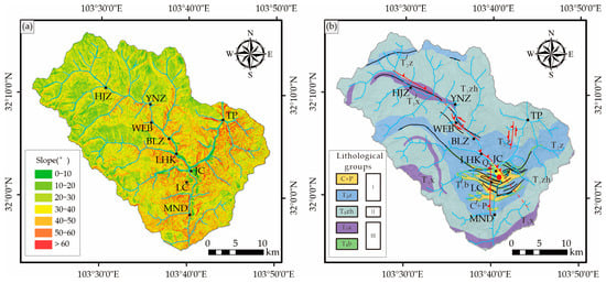
Figure 5.
Maps of (a) slope gradients and (b) lithologic groups. (Detailed parameters are shown in Table 1). The black capitalized letters represent abbreviations for place names as follows: HJZ—Huoji; YNZ—Yini; WEB—Waer; BLZ—Baila; LHK—Lianghe; JC—Jiaochang; LC—Longchi; MND—Manaoding; TP—Taiping.
According to the Standard for the Engineering Classification of Rock Masses, from the General Administration of Quality Supervision of the Ministry of Construction of the People’s Republic of China [37], as well as referring to previous Newmark seismic landslide hazard prediction results for the eastern edge of the Qinghai–Tibet Plateau [34,38], the study area is primarily divided into three lithological groups, corresponding to three distinct levels (Figure 5b). They are (1) Type I (hard rocks), thick-bedded quartz sandstone interbedded with limestone, slate, and phyllite; (2) Type II (moderate hardness rocks), medium-thick-bedded quartz sandstone interbedded with limestone; and (3) Type III (soft rocks), thin-bedded slate and phyllite.
The detailed steps for determining the lithological groups’ parameters are as follows: (1) According to the previously mentioned standard, the regional lithological groups are determined. (2) Based on geological descriptions from geological maps, field investigations, and previous studies, the parameters of the lithological groups, including γ, c, and φ, are preliminarily assigned. These parameters are then verified by those grouped lithological units representing relative rock mass strengths. (3) Steps (1) and (2) are used to repeatedly adjust the lithological strength parameters. This process should be conducted carefully until reasonable parameters are determined [38]. Table 1 shows the obtained lithological parameters used for the landslide hazard estimations.

Table 1.
Representative parameters of engineering geological lithological groups.
2.2.3. Optimization of Newmark Model’s Inputs
The detailed steps for optimizing the Newmark model’s parameters are as follows:
(1) Lithological-group-based slope failure depth: The slope failure depth is generally set as a constant value in many prior Newmark-based studies [33]. We predict Newmark-based landslide hazard susceptibility with a lithological-group-based failure depth to simulate landslides initiating along the lithological face. (2) Slope-structure-based rock mass strength scalar: A previous study on the Diexi Catchment demonstrates that the spatial distribution and susceptibility of earthquake-induced landslides are controlled by slopes’ structural types [28]. It shows that high susceptibility to landslides tends to be located on cataclinal and orthoclinal slopes, indicating the critical importance for incorporating structural effects into earthquake-induced landslide hazard predictions. We define the structure-based cohesion scalar through a 2D wedge slope’s failure-based back-calculation to simulate structural controls on slope stability. (3) Topographic site effects: According to numerical simulations by Meunier et al. [39], seismic waves amplify at ridge tops and slopes’ breakage zones, demonstrating topographic site effects. We consider an amplification scalar at ridge tops beyond the slopes’ breakage zones to simulate topographic site effects caused by seismic waves. (4) Seismically induced strength losses: We consider a reduction scalar of the rock mass strength to compute seismically induced strength losses [4,40].
To simulate the structural effects, a 2D wedge slope stability model is applied to back-calculate the equivalent rock mass strength for each slope’s structural type. This model has been used to back-calculate the equivalent rock mass strength based on the height and slope gradient of hillslopes [35] such that the maximum stable hillslope height is given as follows:
where c is the cohesion, φ is the friction angle, γ is the hillslope’s bulk density, and β is the slope’s gradient. Hillslopes beyond the critical height, Hcrit, have safety factors of <1 and are predicted to fail. The slope-structure-based scalar of cohesion is given as follows:
where Scohesion is a proportional coefficient defined as cstructure divided by clandscape; clandscape is the cohesion of the landscape, based on the height and slope gradient of the entire study area, which determines the level of the landscape-scale rock mass strength; and cstructure is the slope-structure-based cohesion derived from each slope’s structure, such as cataclinal, orthoclinal, and anaclinal hillslopes.
The red curves defining FS = 1 in Figure 6 illustrate that the critical slope height decreases with slope gradient. The results of the back-calculations show the landscape with a cohesion of 44 kPa, the cataclinal slope with a cohesion of 16.2 kPa, the orthoclinal slope with a cohesion of 47.5 kPa, and the anaclinal slope with a cohesion of 60.5 kPa. The corresponding normalized cohesion scalars are 0.37 for the cataclinal slope, 1.08 for the orthoclinal slope, and 1.37 for the anaclinal slope. These values will be used for Newmark-based landslide hazard estimations.
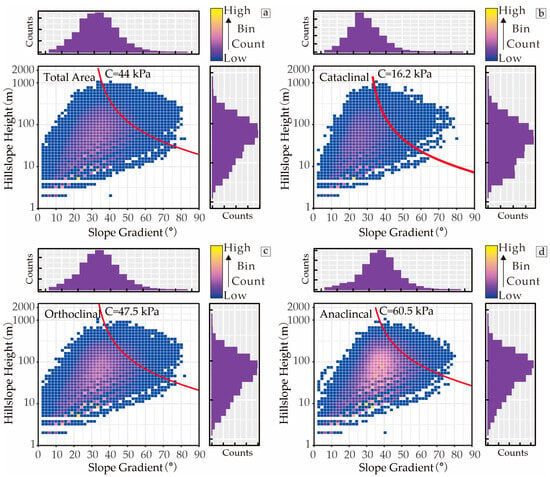
Figure 6.
Back-calculations of different slopes’ structural types in the Diexi Catchment: (a) total study area; (b) cataclinal slope; (c) orthoclinal slope; (d) anaclinal slope.
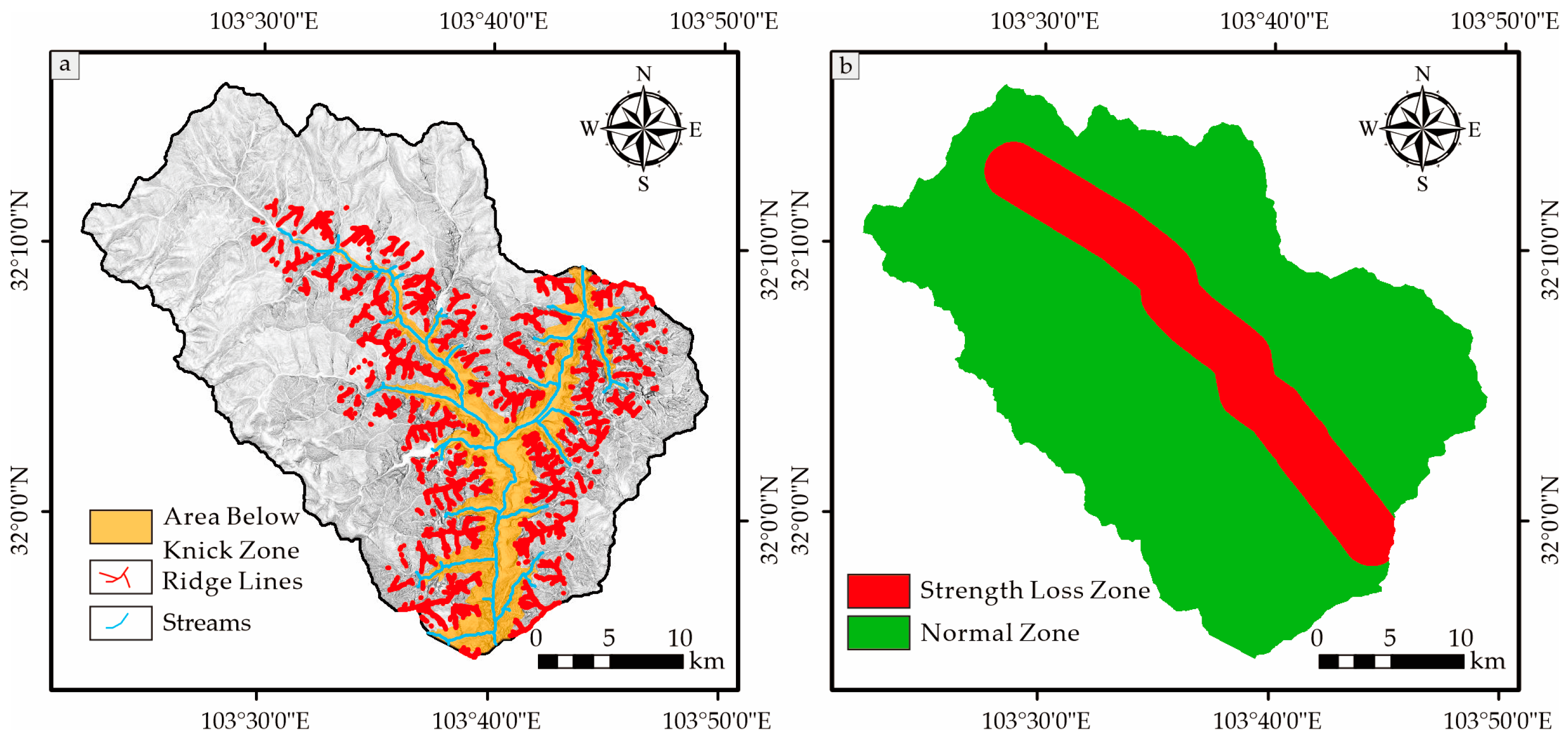
The control of topographic site effects significantly contributes to earthquake-induced landslides. This was demonstrated by numerical simulations of seismic waves propagating through ridges and slope break zones in valley areas [39]. In the Diexi Catchment, this effect is reflected at the ridge top beyond the slope break zones, where landslides cluster [28]. According to prior studies [39,41], we define the amplified areas as ridge tops beyond the slope break zones near the channel within a distance of 2 km, with an amplification scalar of 1.1 (Figure 7a).

Figure 7.
Maps showing the distribution of the amplification factor: (a) topographic amplification; (b) seismically induced strength losses.
The weakening of hillslopes during strong earthquakes increases landsliding rates in post-seismic periods, but very few studies have quantifiably addressed the amount of seismic reduction in the shear strength of hillslope materials [4]. We considered a strength reduction near the Songping Fault within a total distance of 4 km (2 km on each side) based on a prior study [40] (Figure 7b). The latest research shows a maximum reduction from 60 to 75% in the near-surface shear strength over a peak ground acceleration range from 0.5 to 0.9 g, using the 2008 Wenchuan Earthquake in the Longmen Mountain Ranges as an example [4]. Although it indicates a drastic hillslope weakening process, this is the maximum theoretical strength reduction representing a worst-case scenario. Compared with the 2008 MW 7.9 Wenchuan Earthquake, with PGA values between 0.4 and 1.8 g in the meizoseismal area, the 1933 MW 7.3 Diexi Earthquake produced only a maximum PGA of 0.26 g at the epicenter. Therefore, we have reason to believe that the theoretical strength reduction in the Diexi Catchment should be significantly lower than that of the Longmen Mountain Ranges, possibly by an order of magnitude. Considering that both regions are located in similar tectonically active settings, we assumed a seismically induced hillslope strength loss factor of 0.9 for our study, although a precise estimate of the theoretical strength reduction remains uncertain.
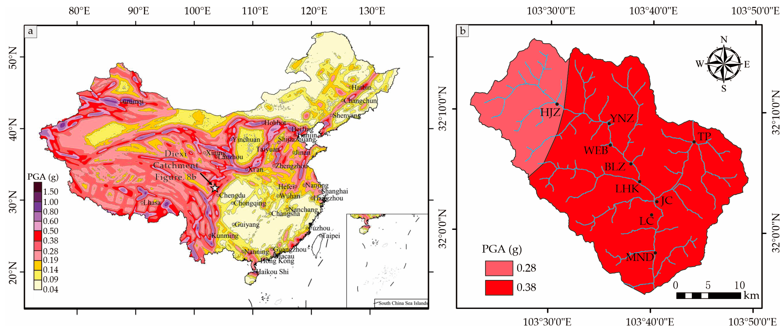
A probabilistic seismic hazard analysis (PSHA) is applied to estimate long-term seismic landslide hazards. PSHA considers the average seismic activity rate within seismic zones and contributions from all the possible source locations [42]. It assumes that earthquakes occur randomly and independently, following a Poisson distribution. PSHA produces a hazard curve of the ground motion parameter, showing an exceedance probability within a future period for a specific location and considering historical seismic activities and seismically induced strength losses [38]. Using PSHA, Chinese experts have developed a method known as the “China Probabilistic Seismic Hazard Analysis” (CPSHA), which fully incorporates the temporal and spatial heterogeneities of seismic activities in China and has been successfully applied in earthquake hazard assessments [43]. To estimate the long-term seismically induced landslide hazards in the Diexi Catchment, we apply the CPSHA approach to create peak ground acceleration (PGA) distribution maps with a 2% exceedance probability in the following 50 years (Figure 8). Figure 8b shows a non-uniform PGA distribution across the study area. However, the area with a PGA value of 0.28 g is relatively small compared to the area with a PGA value of 0.38 g. For simplicity, we approximate the study area as a uniform area with a PGA value of 0.38 g, which is used as the input for our Newmark model.

Figure 8.
Maps showing the PGA with an exceedance probability of 2%. (a) Location of the Diexi Catchment on the CPSHA map. (b) Distribution of the PGA in the Diexi Catchment.
2.2.4. Automatic Extraction of Slope Units
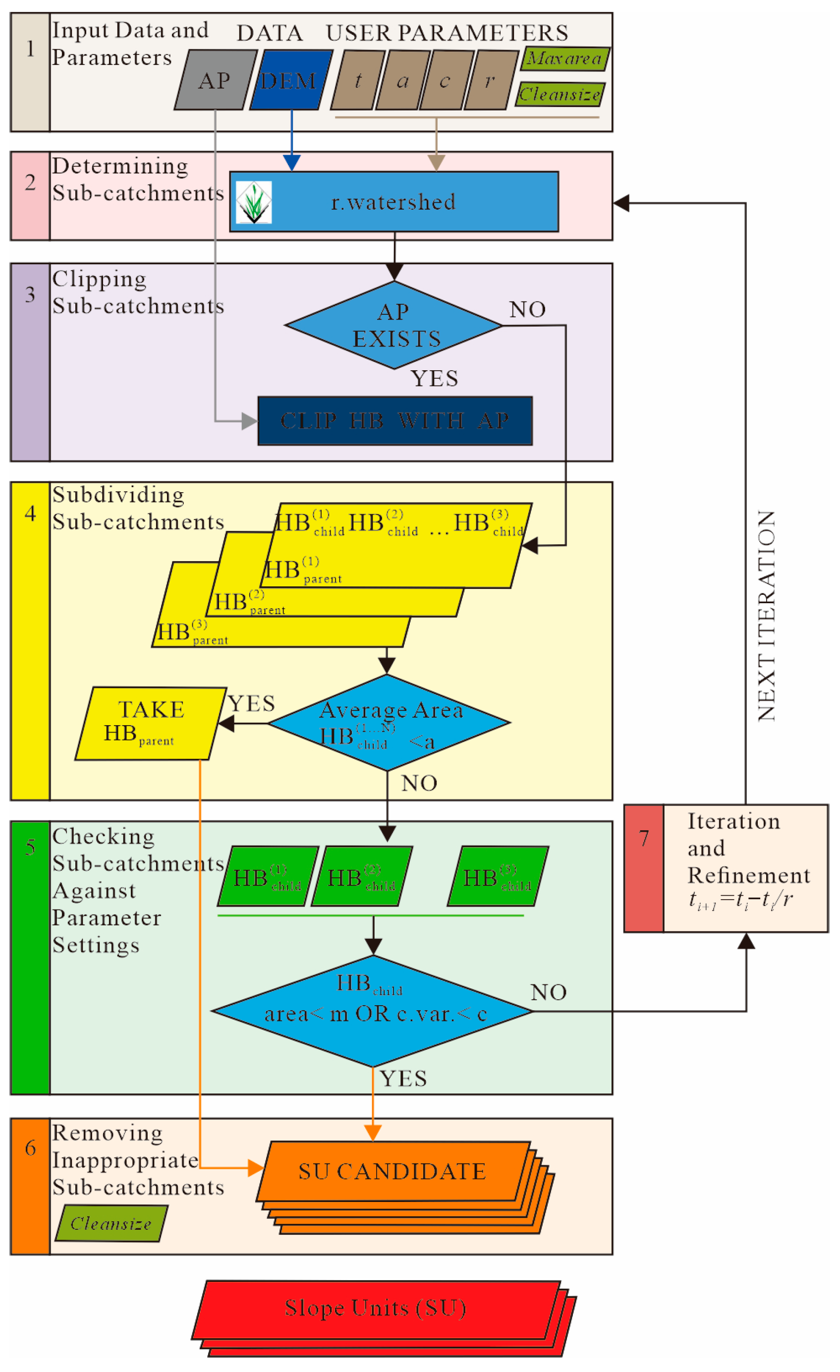
The automatic extraction of slope units was developed by Alvioli et al. [20]. They created the r.slopeunits V1.0 software based on the principle of the maximum homogenization of slope units to ensure a uniform slope aspect. This software can be executed on the open-source GRASSGIS platform. Figure 9 illustrates the detailed steps for the automatic extraction of slope units using the r.slopeunits module as follows:
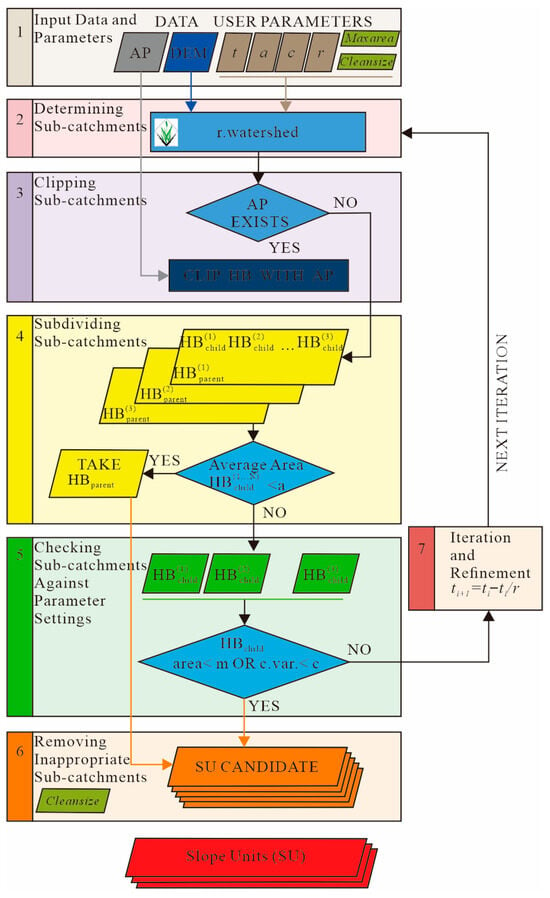
Figure 9.
The flowchart for the automatic extraction of slope units based on r.slopeunits V1.0.
Step 1 (Input data and parameters): The data include the flat terrain’s distribution map (AP) and DEM of the study area. The parameters to be set include the threshold catchment area (t), the minimum area of the slope unit (a), the minimum slope aspect’s difference coefficient within the same slope unit (c), the reduction coefficient (r), the maximum slope unit’s area (maxarea), and the minimum threshold area for removing candidate slope units (cleansize). Step 2 (Determining sub-catchments): The reduction coefficient (t) is used for dividing the study area into several sub-catchments (half-basins, HBs) based on the r.watershed module in the GRASSGIS environment. Step 3 (Clipping sub-catchments): Checking whether the half-basins (HBs) generated in step 2 are located in flat areas. Step 4 (Subdividing sub-catchments): Divide each half-basin (HB) into several half-basins subdividing areas (HB_subs), and compare the average area within the study area with the value of a. If the area of each HB_sub is smaller than a, use the watershed unit (HB); otherwise, proceed to the next step. Step 5 (Checking sub-catchments against parameter settings): Determine whether the area of HB_sub is smaller than a or if the slope aspect’s difference coefficient is less than c. If this condition is met, proceed to step 6; otherwise, go to step 7 for parameter reconfiguration. Step 6 (Removing inappropriate sub-catchments): Based on the results from the previous step, enter the iterative phase to update the initial catchment area threshold. Step 7 (Iteration and refinement): Based on the value of cleansize, remove polygons from the candidate slope unit’s set that are smaller than the threshold. Repeat this process until the subdivision of a sub-watershed is reasonable.
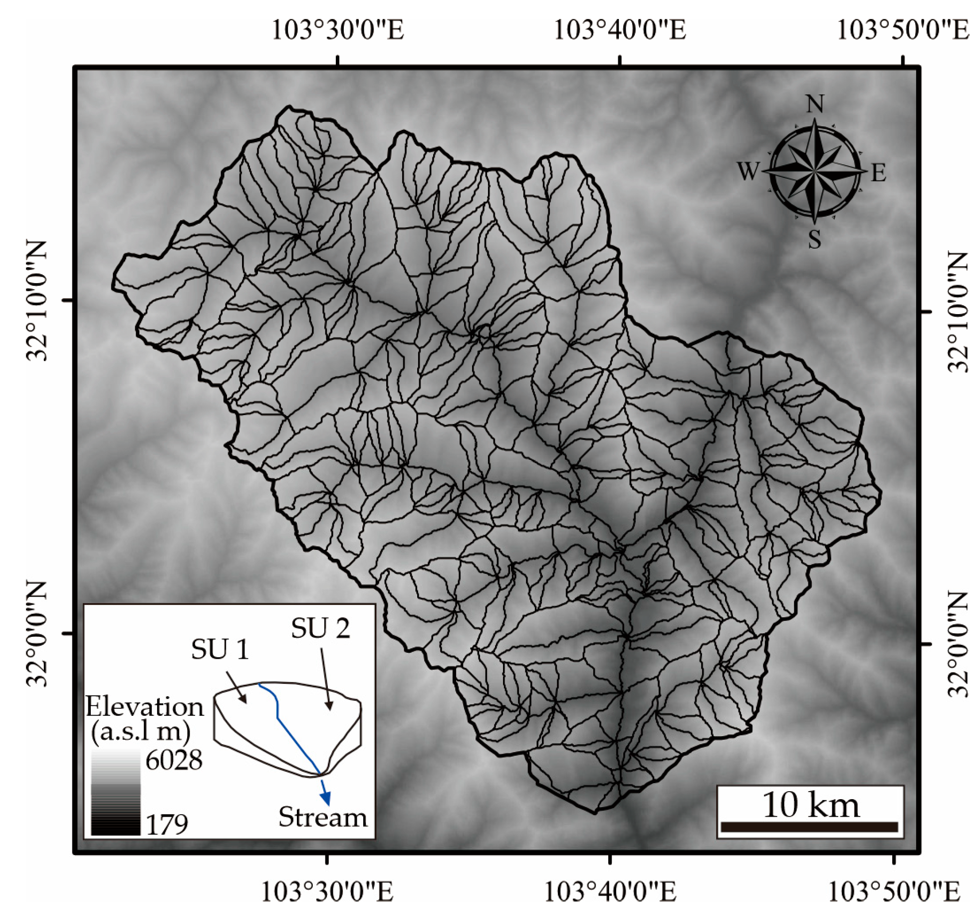
Following the steps mentioned above, a minimum watershed area of 2.7 km2 (cleansize) was used for the SU’s automatic subdivision. The slope units in the Diexi Catchment were ultimately delineated, as shown in Figure 10. The slope units are consistent with the slope aspect, indicating that the subdivision results are reasonable.
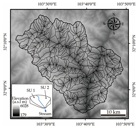
Figure 10.
Automatically generated slope units in the Diexi Catchment.
2.2.5. Procedure of Slope-Unit-Based Landslide Runout
The slope unit enables the sliding direction to be consistent with the direction from the centroid of the landslide source to the nearest channel within the same slope unit, which simulates the natural landslide process under long-term gravitational effects. In the areas within the same slope unit, all the channels modeled as points are given by Pchannel = {P1, P2, …, Pn}, where the 2D coordinates of each channel point (Pi) are (xi,yi), and the coordinates of the landslide centroid (Plandslide) are (xl,yl). The distance (Di) from the landslide centroid to the ith channel point within the same slope unit and the distance to the nearest channel point (Pnearest) are given by the following formulae:
The coordinates of Pnearest are (xn,yn), and the azimuth angle from the landslide centroid to Pnearest is calculated as follows:
where Δx and Δy are the differences between the coordinates of the landslide centroid and the nearest channel, and atan2() is a function to convert arctangent radians to degrees and specifies the sliding direction from the landslide source area to the nearest channel.
The potential source area is approximated as a rectangle, (xr,yr) represent the coordinates of each vertex, and (xm,ym) are post-landsliding coordinates obtained by inputting a given sliding direction (θi) and distance (di) as follows:
Because no available program on various GIS platforms could achieve the above processes, we designed a landslide runout prediction program (Newmark Runout) based on the R and ArcGIS platforms for landslide risk estimations.
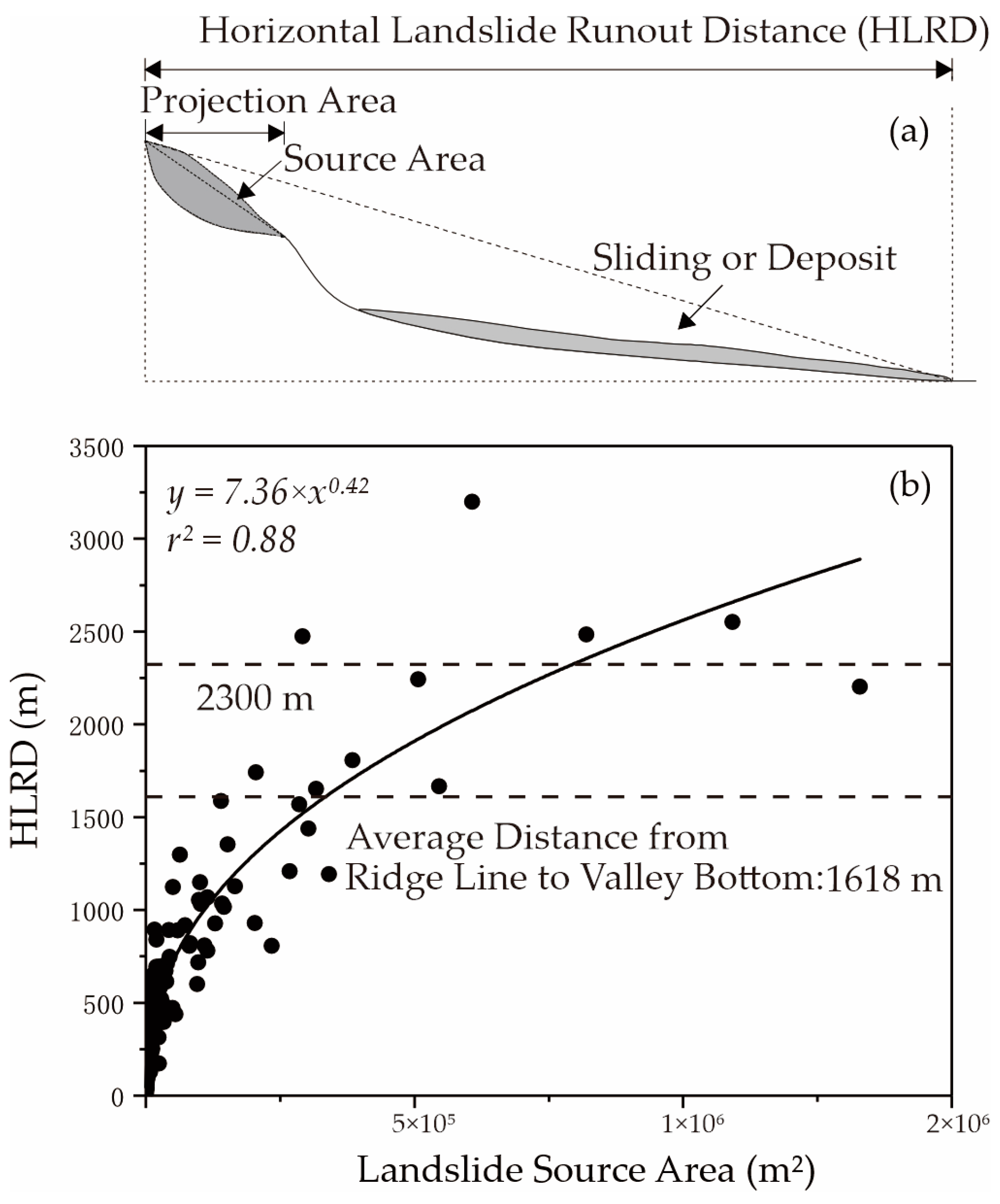
Power-law fitting is commonly used to predict landslide runout distances based on landslide areas or volumes, as the runout distance generally increases with volume [44,45]. However, accurately determining the landslide volume is challenging because of uncertainties in the landslide depth, which may be affected by unknown hidden structures and failure surfaces in the rock mass of hillslopes [46]. Additionally, current predictive parameters are typically derived from observed landslides, making them difficult to implement in a Newmark-based landslide susceptibility model for predicting runout distances. Despite this, we applied power-law fitting in our study to evaluate whether landslide runout distances can be accurately predicted using landslide areas for the Newmark-based model and to determine the maximum runout distance constrained by topographic conditions. Following the methods proposed in previous studies [44,45], we checked the relationship between the landslide area and runout distance in the Diexi Catchment by power-law fitting. Figure 11 shows that the traveling distances of landslides increase with area and that this relationship can be fitted using the formula y = 7.36 × x0.42, with an r2 value of 0.88.
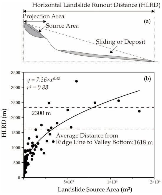
Figure 11.
Illustration of landslide runout and relationship between landslide area and runout distance. (a) Sketch of landslide source area, sliding area, and deposit area; (b) landslide runout distance plotted as a function of the landslide source area for the Diexi Catchment.
This result shows a maximum runout distance of approximately 2300 m, limited by river valleys, as the runout distance tends not to increase significantly beyond this point (Figure 11b). It seems to reach the maximum traveling distance near the valley’s bottom because of the energetic losses caused by topographic impediments. Furthermore, this result also illustrates that although landslide runout distances increase with volume (because volume generally increases with area), the model may underestimate the runout distance because of uncertainties in the landslide failure depth. To address this, we referred to the empirical data from the Wenchuan Earthquake, where landslides blocking channels accounted for 1.6% of the cases [47]. Considering that our study area shares similar geological and topographic features with the Longmen Mountain Ranges, landslides traveling beyond 2300 m accounted for 1.4%, which is nearly consistent with the proportion observed in the Wenchuan Earthquake. Consequently, we estimate that landslide dams, corresponding to 1.4% of the landslides with a maximum runout distance of approximately 2300 m in the Diexi Catchment, are predicted to block channels and form landslide dams.
2.2.6. Kernel-Density-Based Risk Identification
Convolutional-neural-network-based image detection and visual interpretation are combined to map regional infrastructures, such as buildings and roads. After creating a database of vulnerable infrastructures, the kernel density of infrastructures susceptible to seismic landslides will be analyzed. The density analysis of landslides is a commonly used method to estimate landslide hazards and risks. By dividing the number, area, and volume of landslides by the grid-based area, the corresponding point density, areal density, and volumetric density are obtained. These calculations are performed in ArcGIS to reflect landslide intensities, such as the point density or area-weighted density. Ripley’s K-function-based analysis, conducted on the R platform using the spatstat package, determined search radii of 1200 m for buildings and 300 m for roads [48]. These search radii are used for a kernel density function in ArcGIS.
2.2.7. Application and Verification
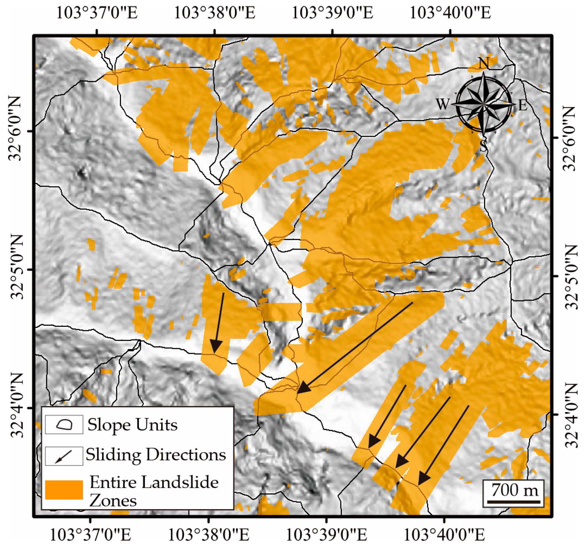
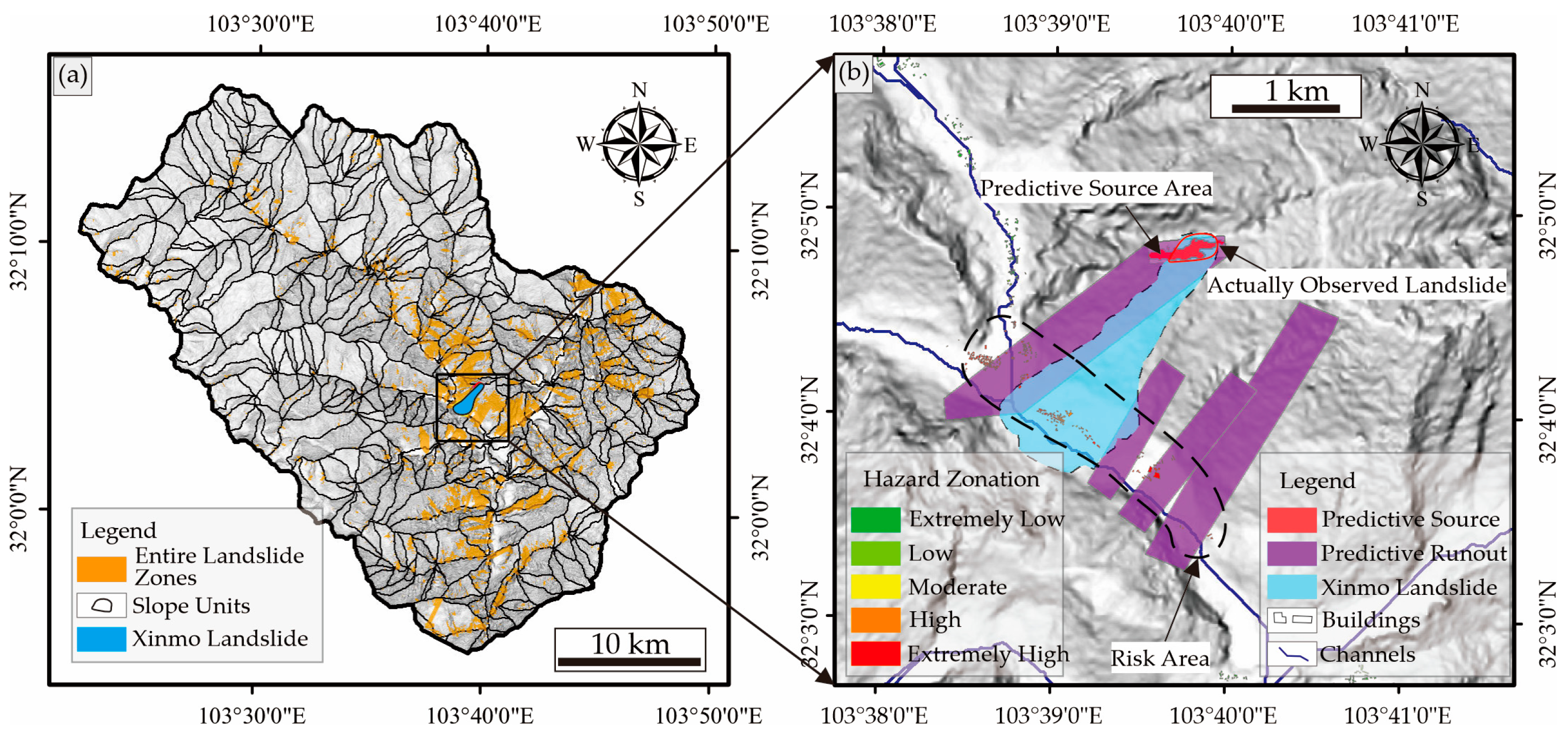
Figure 12 shows that potential landslides initiate in the source area and move to the nearest channel within the same slope unit. This simulates landsliding processes under long-term gravitational influences, demonstrating our model’s effectiveness. Additionally, our prediction follows the Xinmo Landslide’s route, further verifying the accuracy of our landslide runout prediction. However, our model is unable to perfectly predict the entire landslide zone of the Xinmo Landslide (Figure 12), likely because of topographic impediments caused by historical landslides along the sliding path [49]. To address the uncertainty in the sliding direction, we applied distance-weighted kernel density analysis to include areas actually in danger but not covered by the sliding and deposit areas.
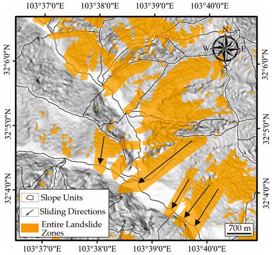
Figure 12.
Illustration of Newmark Runout to predict landslide-covering areas.
The Jenks Natural Breaks Method on the ArcGIS platform is applied to determine the level of the potential distance. Hazard levels are classified by the distance between infrastructures and the nearest potential landslide. Table 2 shows detailed classifications of infrastructural risks, including those to buildings and roads. Using distance-weighted kernel density analysis, hillslopes not covered by landslides but actually in danger are classified as high-risk or extremely high-risk zones (Figure 13).

Table 2.
Hazard levels of infrastructures potentially influenced by landslides. Hazard levels are classified by the distance between infrastructures and the nearest potential landslide.
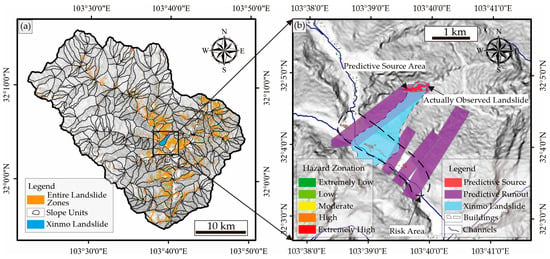
Figure 13.
Slope-unit-based landslide runout hazard prediction: (a) total landslide-covering areas predicted using Newmark Runout for the Diexi Catchment; (b) illustration of distance-based hazard analysis.
3. Results
3.1. Newmark-Based Landslide Hazard Estimations
3.1.1. Generation of the Static Slope Stability and the Critical Acceleration Maps
Following the detailed steps mentioned in Section 2, we input the slope gradient, hillslope strength parameters, failure depth, and optimized topographic site effects into Equations (1) and (2) to generate the static hillslope safety factor (FS) and the critical acceleration (AC), as shown in Figure 14a,b. The static factor of the stability represents a hillslope’s stability under gravitational stress. A higher static safety factor (1.0 < FS < 1.5) indicates a more-stable hillslope. These results illustrate that low-stability zones cluster at the intersection of the Songping River and the Minjiang River, demonstrating the modified model’s capability to simulate topographic site effects. Furthermore, the modified Newmark model incorporates structural effects, enabling the prediction of potential landslides clustering at cataclinal and orthoclinal slopes, particularly on both sides of the Songping Valley. The model’s prediction aligns with the Xinmo Landslide event, proving its effectiveness for Newmark-based landslide hazard prediction influenced by adverse slope structural types, such as cataclinal or orthoclinal slopes. The critical acceleration (AC) indicates the minimum seismic acceleration required to cause slope instability. As shown in Figure 14b, the red areas represent regions with relatively low AC values. These areas are predominantly distributed on the steep slopes around the intersection of the Songping River and the Minjiang River, as well as in regions with cataclinal and orthoclinal slopes. This distribution is consistent with that of FS, indicating that the optimized potential areas with low critical accelerations are more concentrated, reflecting susceptibility to landslide hazards better.
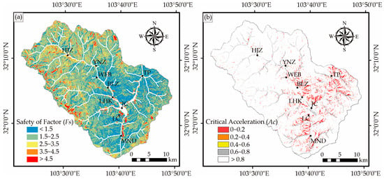
Figure 14.
Maps showing the distributions of the hillslope safety factor and critical acceleration: (a) static hillslope safety factor (FS); (b) critical acceleration (AC). The lower values indicate high susceptibility to landslides.
3.1.2. Landslide Hazard Zonation
The Newmark-based landslide hazard refers to the prediction of potential landslide source areas [32]. The Diexi Catchment was struck by an MW 7.3 earthquake in 1933, which directly triggered most landslides in that region. Previous studies have presented a detailed landslide inventory at the intersection of the Minjiang and the Songping Rivers by interpreting historical ground photographs and current multi-temporal remote-sensing images as well as filed investigations [50,51]. We completed a more-detailed landslide inventory by further interpreting co-seismic landslides distributed along the Songping River [28]. Because of the lack of a pre-seismic DEM (the current DEM version is SRTM 30 m), we cannot directly use the current DEM with the Newmark model to predict landslide susceptibility and evaluate its accuracy. Using a post-seismic DEM to assess the predictive accuracy of co-seismic landslides could lead to logical errors. Therefore, we used the detailed geomorphic footprint and landslide boundaries from this inventory to identify potentially unstable hillslopes that are prone to slope failure in the future but are currently stable.
As shown in Figure 15, these potentially unstable landslide source areas were updated by identifying fresh landslide scars within the landslide boundary, which is used for predictive accuracy testing. The 1933 MW 7.3 Diexi Earthquake triggered landslides covering an area of 44.76 km2 [28] (Figure 15a). The potentially unstable landslide source areas are identified with an area of 4.5 km2. This is comparable to the seismic landslide source area caused by the Diexi Earthquake, which had an area of 7.6 km2 (Figure 15b). These observations verify the identified landslide source area, enabling us to test predictive accuracy by comparing the predictions with the observations.
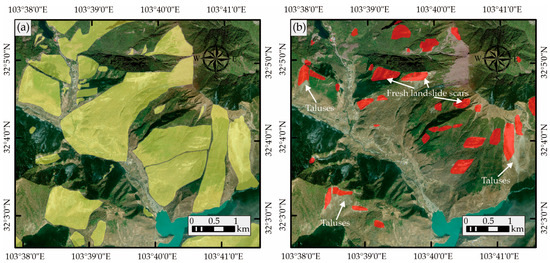
Figure 15.
Comparison of entire landslide zones and landslide source areas. (a) Entire landslide zones induced by the Diexi Earthquake; (b) results of landslide source area interpretation.
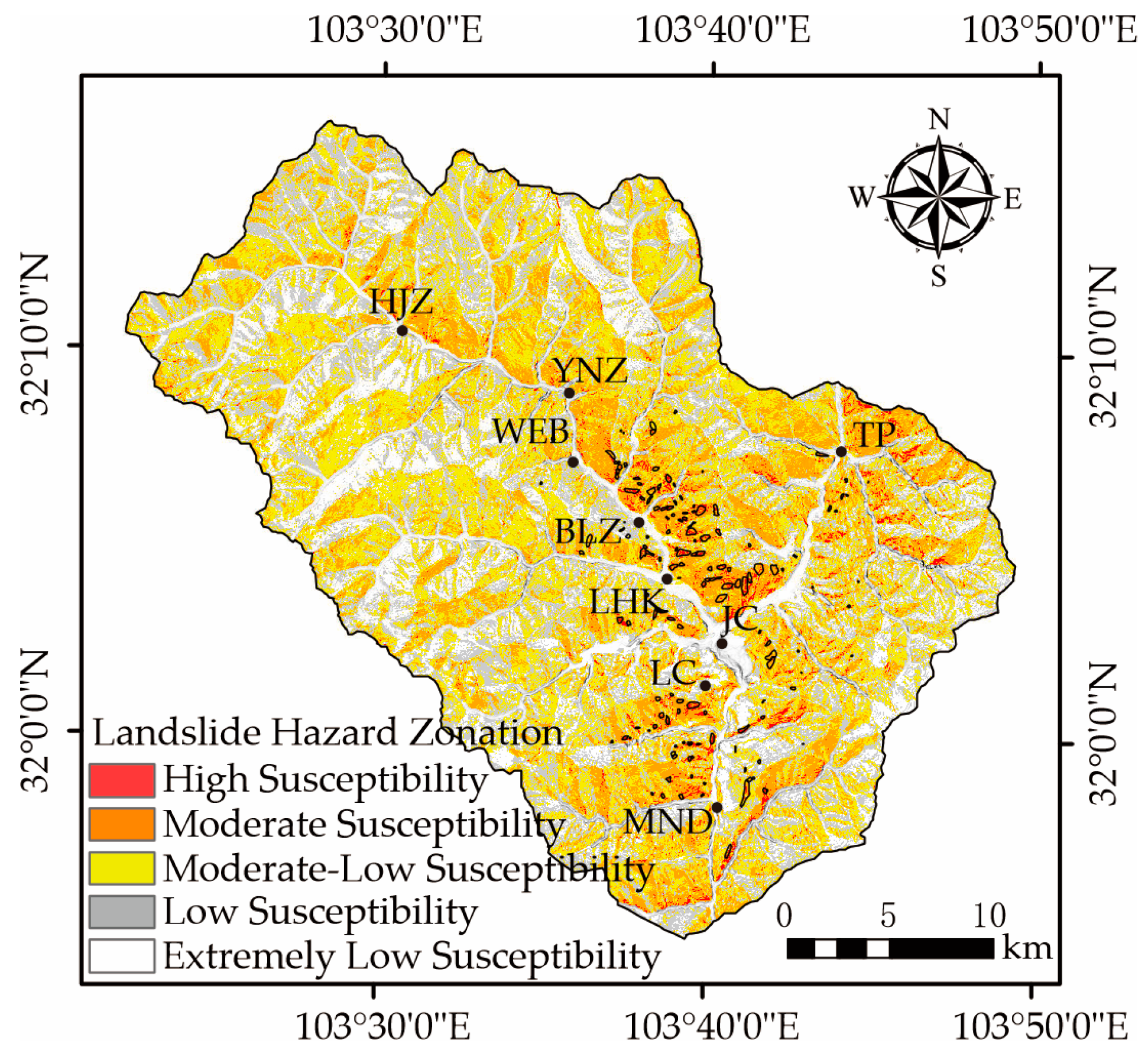
The study area covers 885 km2, and excluding flood plains with slopes below 15° yields 803 km2. After obtaining the results of AC/PGA, the ArcGIS-based Natural Breaks Method was used to determine the landslide susceptibility levels (Table 3). The Natural Breaks Method categorized the susceptibility levels into a high-susceptibility zone (AC/PGA < 4.06), a moderate-susceptibility zone (4.06 < AC/PGA < 14.12), a moderate–low-susceptibility zone (14.12 < AC/PGA < 22.27), a low-susceptibility zone (22.27 < AC/PGA < 30.63), and an extremely low-susceptibility zone (AC/PGA > 30.63). High susceptibility, with AC/PGA values below 4.06, is defined as the potential landslide source area because CPSHA is derived from the level of historical seismic activities in the Diexi Catchment. Figure 16 shows that high-susceptibility zones are predominantly distributed along deeply incised valleys and cataclinal and orthoclinal slopes. This visualization effectively models earthquake-induced landslides caused by topographic site effects, seismically induced rock-mass-strength decreases, and structural influences.

Table 3.
Newmark-based landslide hazard estimation with an exceedance probability of 2%.
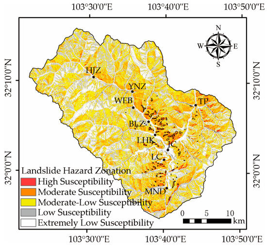
Figure 16.
Susceptibility of landslide source areas based on CPSHA with an exceedance probability of 2%. The inventory of potentially unstable landslide source areas is marked with black boundaries.
Using the formula Slandslides = 9 × 10⁻⁷ × e2.4585×Mw, derived from the statistical data of seismic events between 1980 and 2013, as collected by Xu et al. [52], the predicted entire landslide zone, including both the source and sliding/depositional areas, for the MW 7.3 Diexi Earthquake is approximately 56.04 km2. This is close to the previous landslide inventory, which recorded an area of 44.76 km2, validating our prediction. Therefore, it can be concluded that the theoretical landslide source areas should be about 9.34 km2, considering that the total landslide area is typically six times larger than the landslide source area in the Diexi Earthquake. Table 3 shows that the Newmark-based model, with an exceedance probability of 2%, predicts the potential landslide source area to be 13.47 km2. This is comparable to the theoretical landslide source area of 9.34 km2, demonstrating the robustness of the Newmark-based model.
To present the spatial inconsistency in the prediction of landslide source areas, we added the potential landslide source boundaries in Figure 16 to visualize a comparison of spatial differences between the predicted landslide source areas and the validation dataset. The results show that the spatial discrepancies are primarily located in the northeastern and southern parts of the study area, possibly because these regions are farther from the seismogenic fault, where the rock mass strength has not drastically decreased. This also demonstrates that the seismogenic fault may have caused more damage to the rock mass than initially anticipated.
Besides the visual evaluation, Table 4 quantitatively verifies the modified Newmark model for predicting seismically induced landslide hazards. The proposed Newmark model predicts landslides with an area of 1.53 km2, corresponding to an LFC value of 29.83%. It proves that the proposed Newmark model predicts accurately compared with the general Newmark model (29.83% compared to 5.732%) [11], considering that it is a physical-based model rather than a statistic-based method. Dreyfus et al. [33] explain that the area of false predictions is expected to increase with the total area of the predictions. Thus, the area quantities alone do not reflect the prediction capabilities of a certain approach, which needs to estimate the predictive accuracies concerning both false and true predictions. The predictive accuracy is estimated to reach a value of 97.79%, indicating that the proposed Newmark model estimates fewer landslides but predicts more landslides that are actually unstable in the observations. Consequently, a high-susceptibility landslide model is prepared for the following regional landslide risk estimations, including the infrastructural risk and landslide dam risk analyses:

Table 4.
Efficiency and accuracy of the modified Newmark model at a high-susceptibility level.
3.2. Newmark-Runout-Based Infrastructural Risk Estimations
3.2.1. Risk Estimation of Buildings
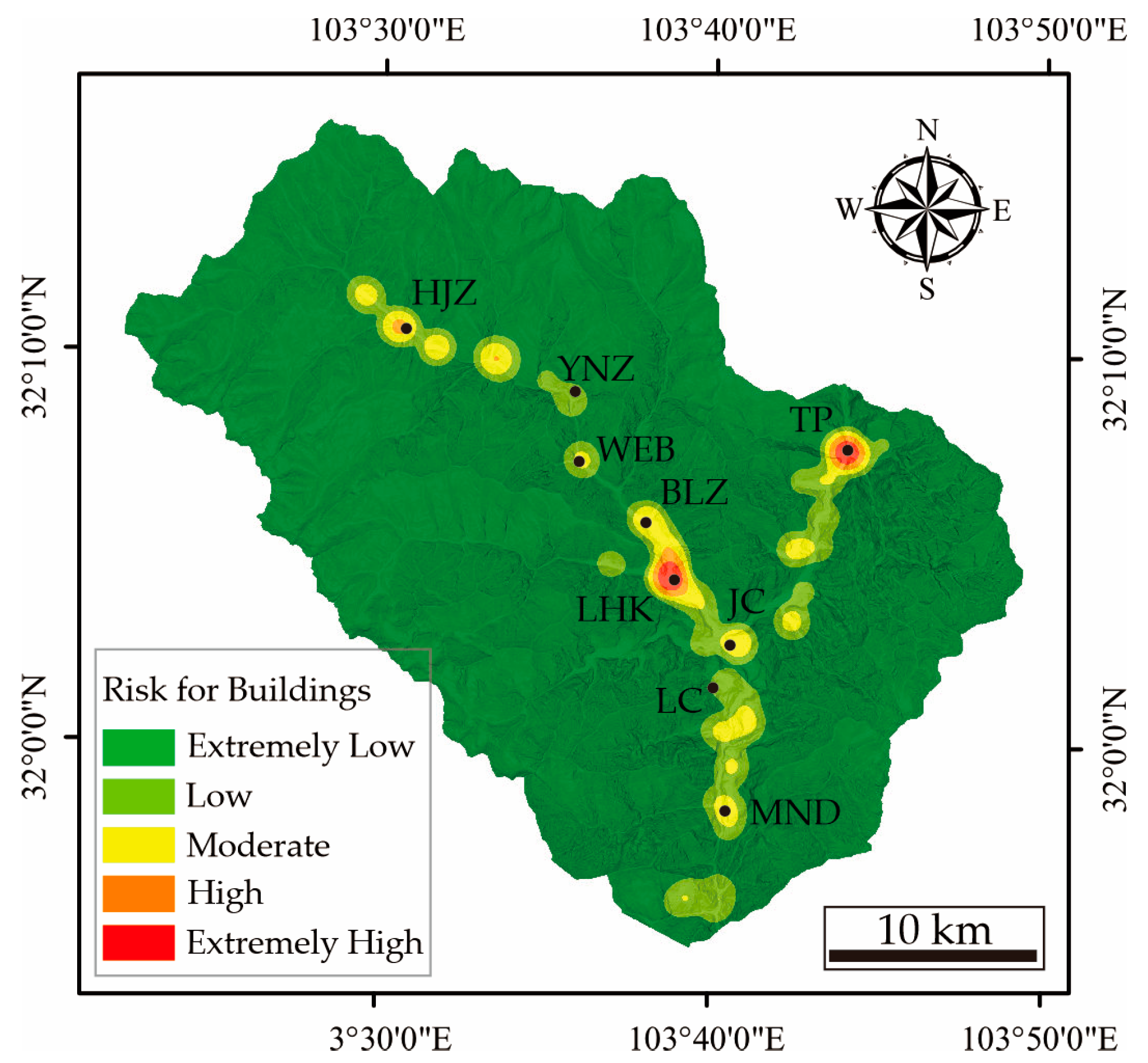
The buildings automatically identified using the convolutional neural network were verified through detailed visual interpretation. Using this method, 2034 buildings were identified in the Diexi Catchment. These buildings were then processed using a GIS platform, calculated, and re-mapped using the kernel density module, with a search radius of 1200 m. The buildings potentially susceptible to landslides were derived and reclassified into five categories using the Natural Breaks Method: extremely high risk, high risk, moderate risk, low risk, and extremely low risk (Figure 17). The potential building risk map indicates that the high-risk and extremely high-risk zones are distributed along the valley, mainly concentrated in the Xinmo and Taiping areas, where potential landslide deposit areas are located near the buildings. In contrast, the buildings in the Jiaochang area are classified as moderate and low risks because they are far from potential landslide deposit areas despite the large number of buildings. The moderate-risk zone also extends downstream of the Jiaochang and Huoji areas.

Figure 17.
Risk estimation of buildings in the Diexi Catchment.
3.2.2. Risk Estimation of Roads
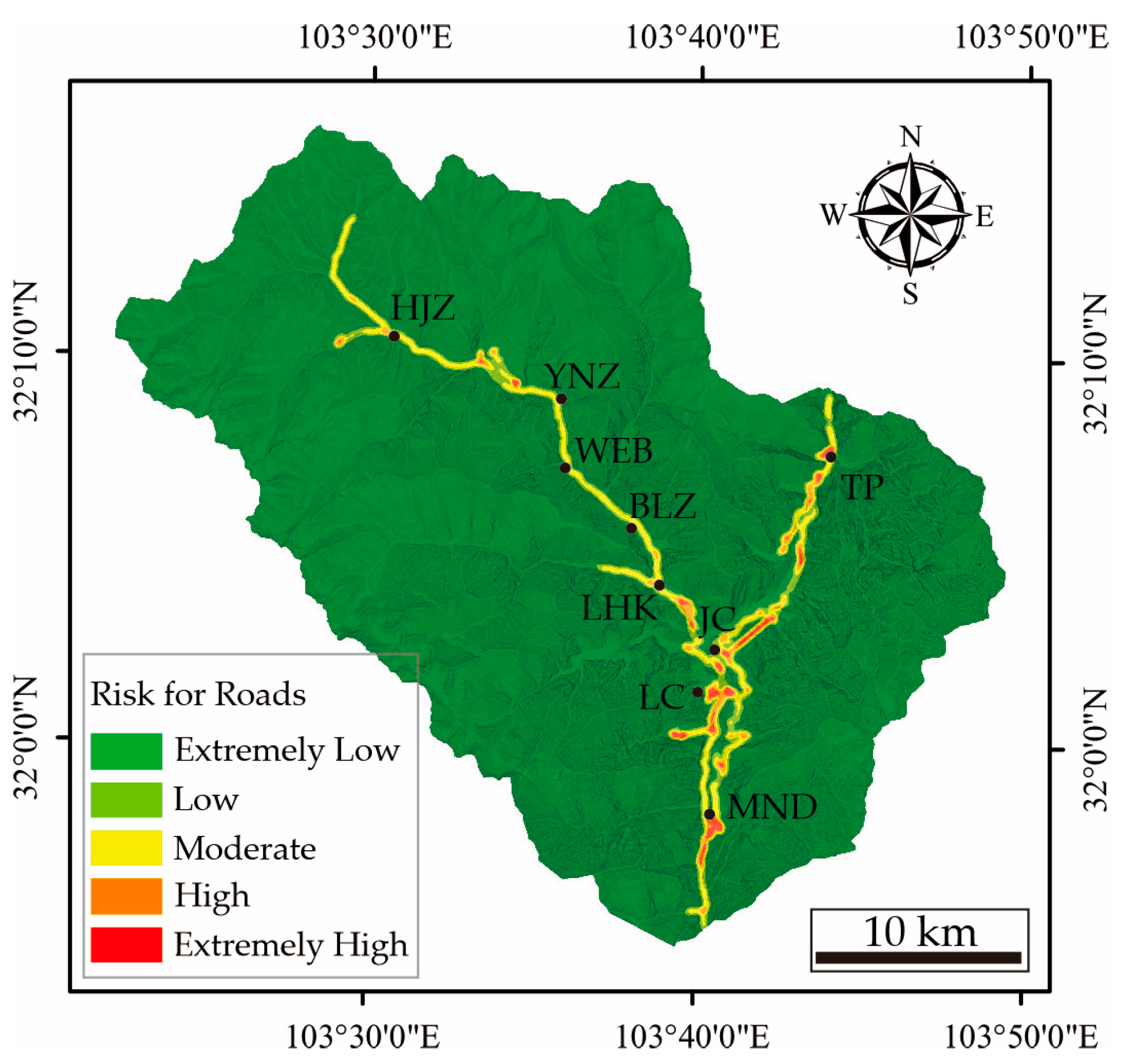
The dataset of roads in the study area is available as open-access data from the Geographic Remote-Sensing Ecological Network Platform (http://gisrs.cn/ accessed on 21 September 2024). These road data are then processed using a GIS-platform-based kernel density module, with a search radius of 300 m. The roads potentially susceptible to landslides are identified and reclassified into five categories using the Natural Breaks Method: extremely high risk, high risk, moderate risk, low risk, and extremely low risk (Figure 18). The potential road risk map indicates that the high-risk and extremely high-risk zones are distributed along the Yingping, Jiaochang, Diexi Tunnel, and Manaoding areas, as well as the Xinmo and Taiping areas, particularly in Jiaochang and Taiping, where the 318 National Highway is well developed.

Figure 18.
Risk estimation of roads in the Diexi Catchment.
3.3. Landslide Dam Risk Estimations
3.3.1. Estimation of Landslide Dam Volume
Landslides triggered by large earthquakes can generate significant volumes of debris that entirely or partially block river channels, leading to catastrophic secondary disasters downstream, such as dam-break floods and debris flows [53]. Therefore, given the tectonically active nature of the Diexi Catchment area, it is critically important for risk estimations to include geohazard chain prevention measures.
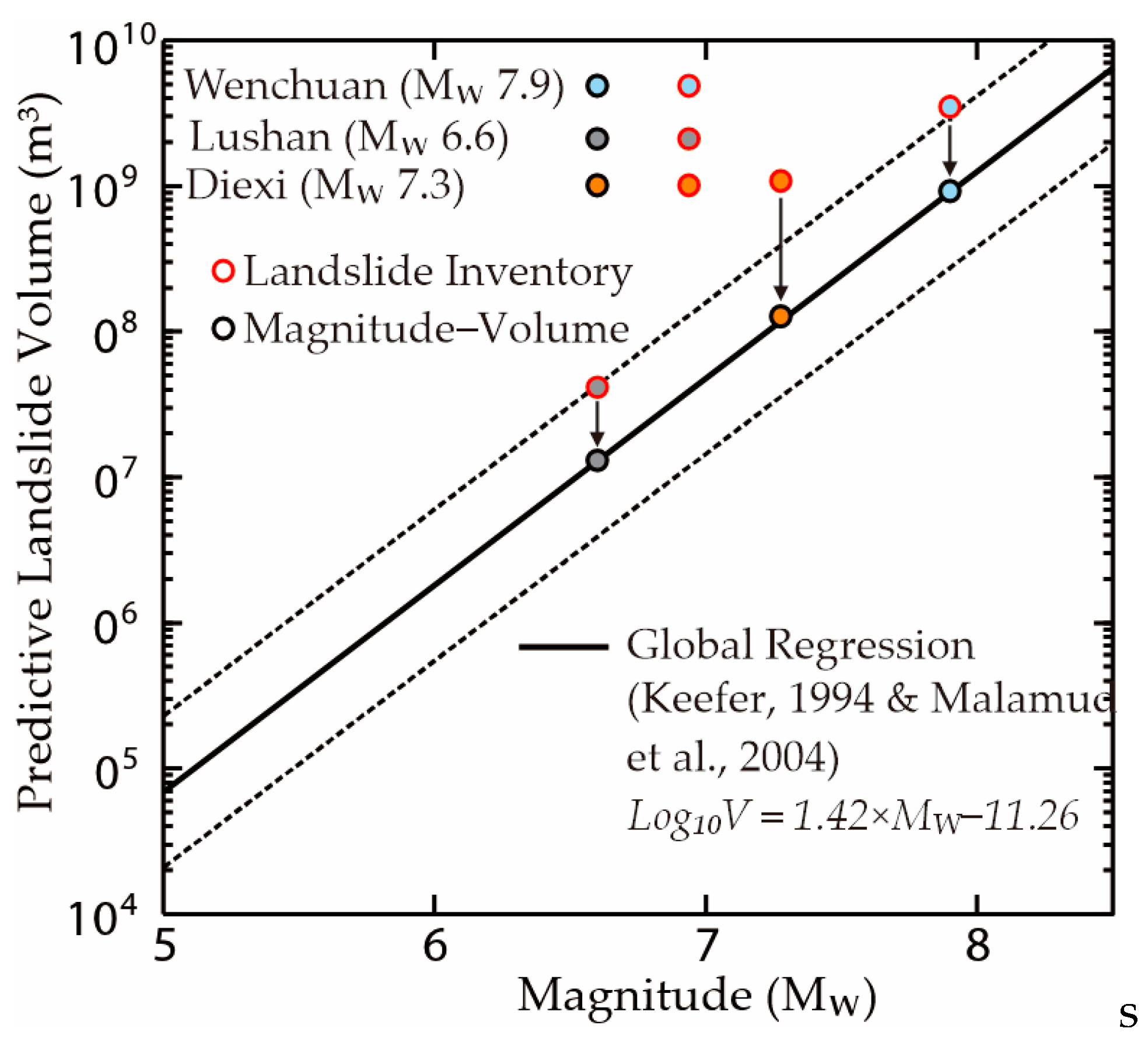
Estimating seismic landslide volumes blocking rivers is crucial for assessing dam-break flood risks. The landslide volume induced by the Diexi Earthquake is calculated using the magnitude–volume and the area–volume formulae. This volume is then compared to the long-term seismic landslide volume derived from the proposed Newmark model, which has a 2% exceedance probability of PGA from CPSHA. The 1933 MW 7.3 Diexi Earthquake resulted in a landslide volume of 0.127 × 10⁹ m3, as estimated using the global magnitude–volume formula (log10VL = 1.42 × MW − 11.26) proposed in previous studies [54,55] (Figure 19). The long-term seismic landslide volume is calculated, yielding a volume of 0.116 × 10⁹ m3 based on parameters proposed in a previous study (log10(α) = −0.63 and γ = 1.41) [56]. The similarity between the long-term seismic landslide volume and the Diexi-Earthquake-induced landslide volume suggests that the long-term seismic landslide volume is related to large earthquakes, like the Diexi Earthquake.
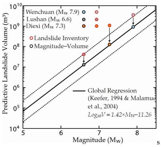
Figure 19.
Earthquake magnitude versus landslide volume based on global empirical regression [54,55].
However, the landslide volume induced by the Diexi Earthquake, as estimated using the magnitude–volume formula, tends to be underestimated. This is because the Diexi Catchment is a rapidly uplifting mountainous area with frequent tectonic activities, which can result in deep-seated landslides and, thus, produce higher landslide volumes than areas with low tectonic activity [8]. This is corroborated by previous studies, which found that magnitude–area-based landslide volumes were four times lower than the landslide-inventory-based landslide volumes for the 2008 MW 7.9 Wenchuan and 2013 MW 6.6 Lushan Earthquakes [8] (Figure 19). According to the landslide inventories from previous studies, the Diexi-Earthquake-induced landslide volume is estimated to be between 1.20 and 1.91 × 10⁹ m3. Despite uncertainties caused by different parameters and landslide interpretations, this estimate is significant by a factor of ten higher than the magnitude–area-based landslide volume estimates [54,55]. This indicates that the estimation of the seismic landslide volume remains considerably uncertain because of the influences of deep-seated structures, seismically induced strength degradation, and undercutting valleys.
Consequently, scalars from 4 to 10 are used as input factors to estimate the range of the seismically induced landslide volume in the Diexi Catchment. By multiplying these scalars, the long-term landslide volume caused by large earthquakes is estimated to be between 0.464 and 1.159 × 10⁹ m3. Referring to the proportion of landslides transforming into landslide dam volumes from previous studies, a transfer rate of 14% is used, resulting in estimated total landslide dam volumes from 0.0649 to 0.162 × 10⁹ m3 in the study area. These match the results estimated in Dai’s study, which found that the largest landslide dams from the 1933 Diexi Earthquake produced total landslide volumes from approximately 0.175 to 0.199 × 10⁹ m3 [50], proving our estimations to be reliable.
3.3.2. Spatial Distribution of Landslide Dams
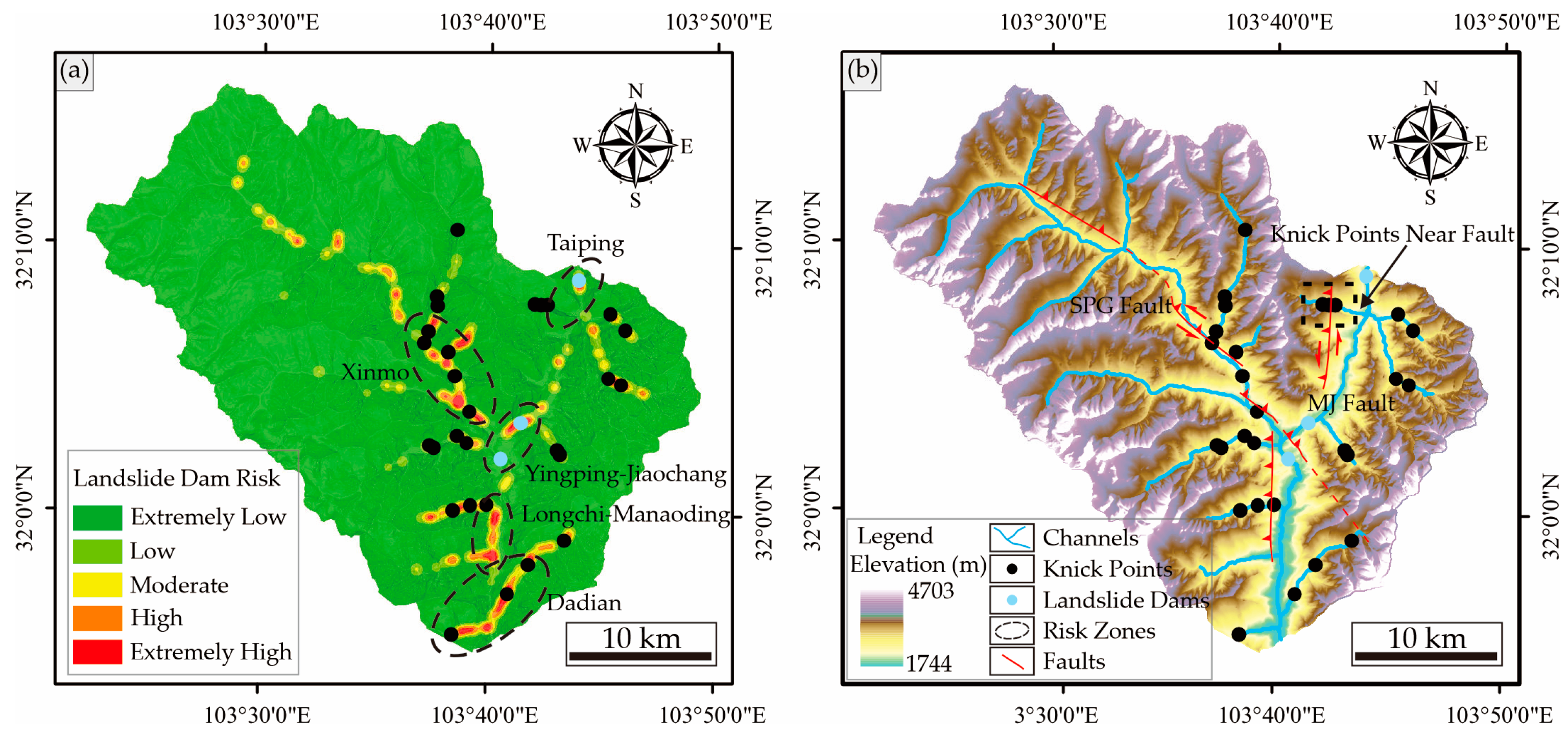
Mapping the spatial distribution of landslide dams is significant for post-seismic cascading-hazard risk estimations. The segments of channels covered by the entire landslide zone, including the sliding and deposit areas, are extracted as points to map the landslide-dam-risk area based on kernel density analysis on a GIS platform (Figure 20). The seismic-landslide-dam-risk map shows that the high-risk and extremely high-risk zones cluster into five main groups: in the Xinmo, Yingping–Jiaochang, Taiping, Longchi–Manaoding, and Dadian areas (Figure 20a). These areas spatially match well with knickpoints, generally thought to be formed by lithologies, landslide dams, and tectonic activities, including faults and tectonic uplifts. Fan et al. [57] conducted a detailed field investigation, illustrating that landslide dams are responsible for these knickpoints (Figure 20b). After excluding three knickpoints near the Minjiang Fault, the number of knickpoints corresponding to the risk zones is assessed as follows: an extremely high-risk zone with eight knickpoints, a high-risk zone with five knickpoints, a moderate-risk zone with eight knickpoints, a low-risk zone with three knickpoints, and an extremely low-risk zone with four knickpoints. The extremely high-risk and high-risk zones have 13 knickpoints, accounting for 50% of the total knickpoints, supporting the reliability of the evaluation outcomes.

Figure 20.
Spatial distribution and risk estimations of seismically induced landslide dams. (a) Risk estimations of landslide dams in the Diexi Catchment. (b) Comparison of landslide dam clustering and knickpoints in the Diexi Catchment.
Streams that tended to be blocked by landslides were identified as those with sufficient flow to form significant impoundments. The Minjiang River is the largest river in the Diexi Catchment. The 1933 Diexi Earthquake caused landslide dams that blocked the river and later breached. The estimated volume of the material released from the three main dams (the Diexi Ancient Town landslide, the Jiaochang landslide, and the upstream Yinpingya rock collapse) is approximately 370.9 × 10⁴ m3. The flood peak propagated at a speed of 26 km/h, affecting areas as far downstream as Xinjin County, 260 km from Diexi [50]. Consequently, we focus on the landslide dam risks of the Minjiang River. The results indicate that in the Minjiang River section, the areas with the highest risk of landslide dams are primarily concentrated in the Yinpingya–Jiaochang area, the Taiping area, and the Longchi–Manaoding area (Figure 21). These areas will require close monitoring in the future for post-earthquake landslide dam risks and dam-break outbursts.
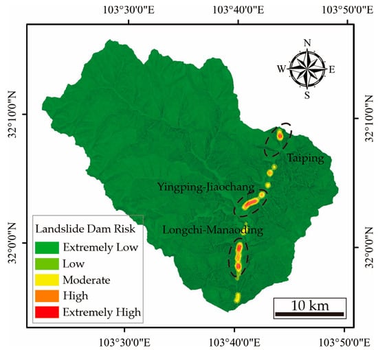
Figure 21.
Risk estimation of landslide dams for the Minjiang River.
4. Discussion
Large earthquakes can directly destroy infrastructures and transiently produce massive landslide volumes, causing severe co-seismic damages and initiating post-seismic geological hazard chains [1]. The risk estimation of seismically induced geohazard chains is complex and crucial for geohazard prediction and prevention. The Newmark model is one of the physical models generally used for earthquake-induced landslide hazard analysis. It rapidly identifies potential landslide source areas by inputting the parameters of slope materials and the peak ground acceleration (PGA). However, few Newmark-based models can predict the landslide sliding or deposition areas, impeding the application of Newmark-based landslide risk estimations.
Efforts for Newmark-based landslide risk estimations have been made in prior studies, but they have not conclusively demonstrated the geomorphic processes by slope units. For instance, one method directly transfers the potential landslide grids within channels to points, enabling landslide dams to be extracted and re-mapped as landslide risk maps based on kernel density analysis [10]. However, this method fails to reflect the actual mechanism because the traditional Newmark model is susceptible to slope gradients. Consequently, kernel density analysis only considering unstable grids near the channel may underestimate the potential landslide risk from ridge tops, especially in tectonically active mountainous areas with significant topographic site effects. Additionally, incorporating rockfall analysis in a Newmark model to obtain a joint procedure is another method to estimate landslide sliding or deposit areas. However, this model predicts the source areas and divides them into grids rather than aggregating them as a total feature, which needs further exploration to be calculated as objectives in rockfall analysis [17].
The slope unit can be topologically defined as a sub-catchment delineated by ridge and valley lines [58,59]. It reflects physical relationships between landslides and morphological features [19,60]. We applied an R-based software package to automatically extract the slope units. Then, we developed an automatic extraction program (Newmark Runout) based on the R platform to model the landslide rushing from the source to the nearest channel within the same slope unit, simulating the landsliding process driven by gravitational effects (Figure 12).
The landslide sliding areas predicted using the Newmark Runout model show that the predictive landslide sliding areas all slide along the direction between the centroid of the source areas and the nearest channel in the same slope unit. The potential source area matches well with that of the 2017 Xinmo Landslide. Additionally, the differences between the north face and the south face of the ridge line are consistent with observations of the Xinmo Landslide. This indicates that incorporating structural effects allows for us to simulate the slope stability of the source area influenced by different structural types, proving our model to be effective. The direction of the predicted sliding is consistent with the initiation of the Xinmo Landslide but shows some bias in the deposit area because the Xinmo Landslide collided with an old landslide at the bottom of the valley, crashing into flow-state rock debris and causing directional deflection [49]. To address the issue of directional bias, distance-based weighting is used in the kernel density module on the GIS platform to avoid excluding low-risk zones that are actually observed to be in danger (Figure 13b). This proves to be effective, as it reclassifies low-risk areas not covered by sliding or deposition areas but near these areas into extremely high-risk or high-risk zones.
Using the proposed Newmark Runout model, risk maps for infrastructures and landslide dams were derived to estimate the seismically induced landslide risk in the Diexi Catchment (Figure 17 and Figure 18). The results show that the highest landslide risk is concentrated at the intersection of the Minjiang and Songping Rivers. High- or extremely high-risk landslide concentrations were modeled for the left bank of the Songping Valley for both buildings and roads. These areas are of concern because landslide geometry modeling results indicate the potential for large landslides influenced by adverse slope structures, deeply incised valleys, and topographic site effects. High population density and primary road access also make these sites of particular concern (Figure 16).
The spatial clustering of landslide dams aligns with field observations and the distribution of knickpoints identified by Fan et al. [47] (Figure 20b), demonstrating the effectiveness of the landslide dam risk estimations. Three areas with a high risk of landslide dams are highlighted in the Minjiang River region: the Taiping area, the Longchi–Manaoding area, and the Songping/Minjiang confluence. These areas potentially produce larger, longer-lived dams potentially presenting a more-significant flood risk.
We emphasize that the proposed Newmark Runout model predicts landslides accurately and provides a potentially useful method to update seismically induced slope stability models. Furthermore, we have provided extensions that estimate infrastructural and landslide dam risks by incorporating geomorphic-process-based slope units in simulating sliding driven by gravitational effects. The proposed model has advantages for simulating landslides, from which the entire landslide zone and post-seismic landslide risk can be evaluated and is easy to implement in the case of few available datasets. Although the results are not meant to estimate the precise locations of landslides actually observed, as the predictive proportion of landslide dams is based on empirical data from Wenchuan-Earthquake-induced landslides in a prior study [47], the landslide failure depth tends to determine the volumes of landslides. In contrast, although the traveling distances of landslides are generally controlled by their volumes [61], to date, no suitable formula exists for Newmark-based landslide area–volume estimations. More research that relates structural densities, structural depths, and landslide areas with volumes, based on the seismic landslide inventory, is needed to fill the knowledge gap in the landslide area–volume-scaling relationship, which is required for accurate landslide risk assessments.
5. Conclusions
The proposed Newmark Runout model improves upon the traditional Newmark model for regional seismically induced landslide risk assessments. The traditional model is limited for predicting the source area based on infinite slope–rigid block analysis, while the Newmark Runout model allows for predicting the entire landslide zone, including sliding and depositional areas that occur after the landslide initiates. To account for the sliding process post failure, a slope-unit-based sliding process from the source area to the deposit area has been developed to simulate the landslide runout process under gravitational effects. Additionally, the proposed model incorporates topographic site effects, seismically induced rock-mass-strength losses, and structural effects for comprehensive seismically induced landslide hazard estimations. Comparisons between the outcomes of the proposed analysis and the potential landslide inventory were made in the Diexi Catchment, Sichuan Province, China. Further verifications were conducted with the prediction of the entire landslide zone and the 2017 Xinmo Landslide. These results demonstrate that the prediction of the whole landslide zone, including the landslide source area and sliding/depositional areas, is accurately achieved using the proposed Newmark Runout approach. Quantitative measurements indicate that the proposed model efficiently predicts landslides by comparing predictions with observations. Based on the hazard analysis of the entire landslide zone, seismically induced infrastructural risks in the study area have been estimated by analyzing the risks to buildings and roads. Finally, the volume of landslides blocking river channels was assessed, and landslide-dam-risk zoning in the Diexi Catchment was evaluated.
Author Contributions
Conceptualization, H.W.; methodology, H.W. and C.Y.; formal analysis, H.W. and H.Y.; writing—original draft preparation, H.W. and C.Y.; writing—review and editing, T.O. and Z.H.; visualization, C.Y. and H.Y.; supervision, X.P.; project administration, X.P.; funding acquisition, X.P. and R.H. All authors have read and agreed to the published version of the manuscript.
Funding
This research was partly supported by the National Natural Science Foundation of China (Grants No. 41931296 and 41521002) and the National Key R&D Program of China (Grant No. 2017YFC1501002). The first author is financially supported by the China Scholarship Council (Grant No. 202208510134).
Data Availability Statement
The data presented in this study are available on request.
Acknowledgments
We sincerely thank Chengquan Zhang, at the University of Tokyo, Japan, for his constructive comments and thoughtful suggestions about computations and programming. We also appreciate Xiaotian Cao, at Hunan University of Science and Technology, China, for the technical support.
Conflicts of Interest
The authors declare no conflicts of interest. The funders had no role in the design of the study; in the collection, analyses, or interpretation of the data; in the writing of the manuscript; or in the decision to publish the results.
References
- Fan, X.M.; Scaringi, G.; Korup, O.; West, A.J.; Van Westen, C.J.; Tanyas, H.; Hovius, N.; Hales, T.C.; Jibson, R.W.; Allstadt, K.E.; et al. Earthquake-Induced Chains of Geologic Hazards: Patterns, Mechanisms, and Impacts. Rev. Geophys. 2019, 57, 421–503. [Google Scholar] [CrossRef]
- Cui, P.; Ge, Y.; Li, S.; Li, Z.; Xu, X.; Zhou, G.; Chen, H.; Wang, H.; Lei, Y.; Zhou, L.; et al. Scientific challenges in disaster risk reduction for the Sichuan–Tibet Railway. Eng. Geol. 2020, 309, 106837. [Google Scholar] [CrossRef]
- Xu, C.; Xu, X.W.; Yao, X.; Dai, F.C. Three (nearly) complete inventories of landslides triggered by the May 12, 2008 Wenchuan Mw 7.9 earthquake of China and their spatial distribution statistical analysis. Landslides 2014, 11, 441–461. [Google Scholar] [CrossRef]
- Xi, C.; Tanyas, H.; Lombardo, L.; He, K.; Hu, X.; Jibson, R. Estimating weakening on hillslopes caused by strong earthquakes. Commun. Earth Environ. 2024, 5, 81. [Google Scholar] [CrossRef]
- Yi, S.; Wu, C.; Cui, P.; Li, Y.; Lei, M. Cause of the Baige Landslides: Long-Term Cumulative Coupled Effect of Tectonic Action and Surface Erosion. Lithosphere 2022, 7, 7784535. [Google Scholar] [CrossRef]
- Livio, F.; Ferrario, M.F. Assessment of attenuation regressions for earthquake-triggered landslides in the Italian Apennines: Insights from recent and historical events. Landslides 2020, 17, 2825–2836. [Google Scholar] [CrossRef]
- Fan, X.M.; Domenech, G.; Scaringi, G.; Huang, R.Q.; Xu, Q.; Hales, T.; Dai, L.X.; Yang, Q.; Francis, O. Spatio-temporal evolution of mass wasting after the 2008 M-w 7.9 Wenchuan earthquake revealed by a detailed multi-temporal inventory. Landslides 2018, 15, 2325–2341. [Google Scholar] [CrossRef]
- Li, G.; West, A.J.; Densmore, A.L.; Jin, Z.; Zhang, F.; Wang, J.; Clark, M.; Hilton, R.G. Earthquakes drive focused denudation along a tectonically active mountain front. Earth Planet. Sci. Lett. 2017, 472, 253–265. [Google Scholar] [CrossRef]
- Ma, S.; Xu, C.; Shao, X. Spatial prediction strategy for landslides triggered by large earthquakes oriented to emergency response, mid-term resettlement and later reconstruction. Int. J. Disaster Risk Reduct. 2020, 43, 101362. [Google Scholar] [CrossRef]
- Gallen, S.; Clark, M.; Godt, J.; Roback, K.; Niemi, N. Application and evaluation of a rapid response earthquake-triggered landslide model to the 25 April 2015 Mw 7.8 Gorkha earthquake, Nepal. Tectonophysics 2016, 714, 173–187. [Google Scholar] [CrossRef]
- Saade, A.; Abou-Jaoude, G.; Wartman, J. Regional-scale co-seismic landslide assessment using limit equilibrium analysis. Eng. Geol. 2016, 204, 53–64. [Google Scholar] [CrossRef]
- Grant, A.; Wartman, J.; Abou-Jaoude, G. Multimodal method for coseismic landslide hazard assessment. Eng. Geol. 2016, 212, 146–160. [Google Scholar] [CrossRef]
- Newmark, N. Effects of Earthquakes on Dams and Embankments. Geotechnique 1965, 15, 139–160. [Google Scholar] [CrossRef]
- Jibson, R.W. Predicting earthquake-induced landslide displacements using Newmark’s sliding block analysis. Transp. Res. Rec. 1993, 1411, 9–17. [Google Scholar]
- Hungr, O.; Leroueil, S.; Picarelli, L. The Varnes classification of landslide types, an update. Landslides 2014, 11, 167–194. [Google Scholar] [CrossRef]
- Peng, W.F.; Wang, C.L.; Chen, S.T.; Lee, S.T. Incorporating the effects of topographic amplification and sliding areas in the modeling of earthquake-induced landslide hazards, using the cumulative displacement method. Comput. Geosci. 2009, 35, 946–966. [Google Scholar] [CrossRef]
- Yue, X.L.; Wu, S.H.; Yin, Y.H.; Gao, J.B.; Zheng, J.Y. Risk Identification of Seismic Landslides by Joint Newmark and RockFall Analyst Models: A Case Study of Roads Affected by the Jiuzhaigou Earthquake. Int. J. Disaster Risk Sci. 2018, 9, 392–406. [Google Scholar] [CrossRef]
- Huang, F.M.; Tao, S.Y.; Chang, Z.L.; Huang, J.S.; Fan, X.M.; Jiang, S.H.; Li, W.B. Efficient and automatic extraction of slope units based on multi-scale segmentation method for landslide assessments. Landslides 2021, 18, 3715–3731. [Google Scholar] [CrossRef]
- Alvioli, M.; Guzzetti, F.; Marchesini, I. Parameter-free delineation of slope units and terrain subdivision of Italy. Geomorphology 2020, 358, 107124. [Google Scholar] [CrossRef]
- Alvioli, M.; Marchesini, I.; Reichenbach, P.; Rossi, M.; Ardizzone, F.; Fiorucci, F.; Guzzetti, F. Automatic delineation of geomorphological slope units with r.slopeunits v1.0 and their optimization for landslide susceptibility modeling. Geosci. Model Dev. 2016, 9, 3975–3991. [Google Scholar] [CrossRef]
- Deng, B.; Liu, S.G.; Liu, S.; Li, Z.W. The micro-strain mechanism of Jiaochang arc structure in Songpan-Garze fold belt, Sichuan, China. Geol. Bull. China 2010, 29, 697–706. (In Chinese) [Google Scholar]
- Cook, K.L.; Royden, L.H.; Burchfiel, B.C.; Lee, Y.-H.; Tan, X. Constraints on Cenozoic tectonics in the southwestern Longmen Shan from low-temperature thermochronology. Lithosphere 2013, 5, 393–406. [Google Scholar] [CrossRef]
- Chen, Y.L.; Li, D.P.; Zhou, J.; Liu, F.; Zhang, H.F.; Nie, L.S.; Jiang, L.T.; Song, B.; Liu, X.M.; Wang, Z. U-Pb dating, geochemistry, and tectonic implications of the Songpan-Ganzi block and the Longmen Shan, China. Geochem. J. 2009, 243, 77–99. [Google Scholar] [CrossRef]
- Li, Y.; Cao, S.; Zhou, R.; Densmore, A.L.; Aellis, M. Late Cenozoic Minjiang Incision Rate and Its Constraint on the Uplift of the Eastern Margin of the Tibetan Plateau. Acta Geol. Sin. 2005, 79, 28–37. [Google Scholar] [CrossRef]
- Zhao, S.; Chigira, M.; Wu, X. Gigantic rockslides induced by fluvial incision in the Diexi area along the eastern margin of the Tibetan Plateau. Geomorphology 2019, 338, 27–42. [Google Scholar] [CrossRef]
- Xu, Z.Q.; Hou, L.W.; Wang, Z.X. Mountain Building Processes of the Songpan-Ganzi Orogency; Geological Publishing House: Beijing, China, 1992. (In Chinese) [Google Scholar]
- Shao, C.J.; Li, Y.; Lan, H.X.; Li, P.Y.; Zhou, R.J.; Ding, H.R.; Yan, Z.K.; Dong, S.L.; Yan, L.; Deng, T. The role of active faults and sliding mechanism analysis of the 2017 Maoxian postseismic landslide in Sichuan, China. Bull. Eng. Geol. Environ. 2019, 78, 5635–5651. [Google Scholar] [CrossRef]
- Cui, S.H.; Wu, H.; Pei, X.J.; Yang, Q.W.; Huang, R.Q.; Guo, B. Characterizing the spatial distribution, frequency, geomorphological and geological controls on landslides triggered by the 1933 Mw 7.3 Diexi Earthquake, Sichuan, China. Geomorphology 2022, 403, 108177. [Google Scholar] [CrossRef]
- Chen, J.H.; Liu, Q.Y.; Li, S.C.; Guo, B.; Wang, J.; Qi, S.H. Seismotectonic study by relocation of the Wenchuan M(S)8.0 earthquake sequence. Chin. J. Geophys. Chin. Ed. 2009, 52, 390–397. (In Chinese) [Google Scholar]
- Jones, L.M.; Han, W.; Hauksson, E.; Jin, A.; Zhang, Y.; Luo, Z. Focal mechanisms and aftershock locations of the Songpan earthquakes of August 1976 in Sichuan, China. J. Geophys. Res. Solid Earth 1984, 89, 7697–7707. [Google Scholar] [CrossRef]
- Huang, Z.; Tang, R.; Liu, S. Re-discussion of the Seismogenic Structure of the Diexi Large Earthquake in 1933 and the Arc Tectonics on Jiaochang, Sichuan Province. Earthq. Res. China 2002, 18, 183–192. [Google Scholar] [CrossRef]
- Jibson, R.; Harp, E.; Michael, J. A method for producing digital probabilistic seismic landslide hazard maps. Eng. Geol. 2000, 58, 271–289. [Google Scholar] [CrossRef]
- Dreyfus, D.; Rathje, E.M.; Jibson, R.W. The influence of different simplified sliding-block models and input parameters on regional predictions of seismic landslides triggered by the Northridge earthquake. Eng. Geol. 2013, 163, 41–54. [Google Scholar] [CrossRef]
- Chen, X.L.; Liu, C.G.; Yu, L.; Lin, C.X. Critical acceleration as a criterion in seismic landslide susceptibility assessment. Geomorphology 2014, 217, 15–22. [Google Scholar] [CrossRef]
- Gallen, S.F.; Clark, M.K.; Godt, J.W. Coseismic landslides reveal near-surface rock strength in a high-relief, tectonically active setting. Geology 2015, 43, 11–14. [Google Scholar] [CrossRef]
- Chen, L.X.; Mei, L.; Zeng, B.; Yin, K.L.; Shrestha, D.P.; Du, J. Failure probability assessment of landslides triggered by earthquakes and rainfall: A case study in Yadong County, Tibet, China. Sci. Rep. 2020, 10, 16531. [Google Scholar] [CrossRef]
- GB/T 50218-2014; Standard for Engineering Classification of Rock Mass. Standards Press of China: Beijing, China, 2014. (In Chinese)
- Li, C.; Su, L.J. Influence of critical acceleration model on assessments of potential earthquake-induced landslide hazards in Shimian County, Sichuan Province, China. Landslides 2021, 18, 1659–1674. [Google Scholar] [CrossRef]
- Meunier, P.; Hovius, N.; Haines, J. Topographic site effects and the location of earthquake induced landslides. Earth Planet. Sci. Lett. 2008, 275, 221–232. [Google Scholar] [CrossRef]
- Kirkpatrick, H.M.; Moon, S.; Yin, A.; Harrison, T.M. Impact of fault damage on eastern Tibet topography. Geology 2021, 49, 30–34. [Google Scholar] [CrossRef]
- Dunham, A.; Kiser, E.; Kargel, J.; Haritashya, U.; Watson, C.S.; Shugar, D.; Hughes, A.; DeCelles, P. Topographic Control on Ground Motions and Landslides From the 2015 Gorkha Earthquake. Geophys. Res. Lett. 2022, 49, e2022GL098582. [Google Scholar] [CrossRef]
- Caccavale, M.; Matano, F.; Sacchi, M. An integrated approach to earthquake-induced landslide hazard zoning based on probabilistic seismic scenario for Phlegrean Islands (Ischia, Procida and Vivara), Italy. Geomorphology 2017, 295, 235–259. [Google Scholar] [CrossRef]
- Xu, W.; Wu, J.; Gao, M. Seismic Hazard Analysis of China’s Mainland Based on a New Seismicity Model. Int. J. Disaster Risk Sci. 2023, 14, 280–297. [Google Scholar] [CrossRef]
- Legros, F. The mobility of long-runout landslides. Eng. Geol. 2002, 63, 301–331. [Google Scholar] [CrossRef]
- Crosta, G.B.; De Blasio, F.V.; Frattini, P. Global Scale Analysis of Martian Landslide Mobility and Paleoenvironmental Clues. J. Geophys. Res. Planets 2018, 123, 872–891. [Google Scholar] [CrossRef]
- Larsen, I.J.; Montgomery, D.R.; Korup, O. Landslide erosion controlled by hillslope material. Nat. Geosci. 2010, 3, 247–251. [Google Scholar] [CrossRef]
- Fan, X.; Van Westen, C.J.; Korup, O.; Gorum, T.; Xu, Q.; Dai, F.; Huang, R.; Wang, G. Transient water and sediment storage of the decaying landslide dams induced by the 2008 Wenchuan earthquake, China. Geomorphology 2012, 171, 58–68. [Google Scholar] [CrossRef]
- Baddeley, A.; Turner, R. Spatstat: An R package for analyzing spatial point patterns. J. Stat. Softw. 2005, 12, 1–42. [Google Scholar] [CrossRef]
- Huang, D.; Li, Y.Q.; Song, Y.X.; Xu, Q.; Pei, X.J. Insights into the catastrophic Xinmo rock avalanche in Maoxian county, China: Combined effects of historical earthquakes and landslide amplification. Eng. Geol. 2019, 258, 105158. [Google Scholar] [CrossRef]
- Dai, L.X.; Fan, X.M.; Jansen, J.D.; Xu, Q. Landslides and fluvial response to landsliding induced by the 1933 Diexi earthquake, Minjiang River, eastern Tibetan Plateau. Landslides 2021, 18, 3011–3025. [Google Scholar] [CrossRef]
- Zhao, S.; Chigira, M.; Wu, X. Buckling deformations at the 2017 Xinmo landslide site and nearby slopes, Maoxian, Sichuan, China. Engineering Geology 2018, 246, 187–197. [Google Scholar] [CrossRef]
- Xu, C.; Xu, X.; Shyu, J.B.H. Database and spatial distribution of landslides triggered by the Lushan, China Mw 6.6 earthquake of 20 April 2013. Geomorphology 2015, 248, 77–92. [Google Scholar] [CrossRef]
- Li, G.; West, A.J.; Densmore, A.L.; Hammond, D.E.; Jin, Z.; Zhang, F.; Wang, J.; Hilton, R.G. Connectivity of earthquake-triggered landslides with the fluvial network: Implications for landslide sediment transport after the 2008 Wenchuan earthquake. J. Geophys. Res. Earth Surf. 2016, 121, 703–724. [Google Scholar] [CrossRef]
- Keefer, D.K. The importance of earthquake-induced landslides to long-term slope erosion and slope-failure hazards in seismically active regions. Geomorphology 1994, 10, 265–284. [Google Scholar] [CrossRef]
- Malamud, B.D.; Turcotte, D.L.; Guzzetti, F.; Reichenbach, P. Landslide inventories and their statistical properties. Earth Surf. Process. Landf. 2004, 29, 687–711. [Google Scholar] [CrossRef]
- Parker, R.N.; Densmore, A.L.; Rosser, N.J.; De Michele, M.; Li, Y.; Huang, R.Q.; Whadcoat, S.; Petley, D.N. Mass wasting triggered by the 2008 Wenchuan earthquake is greater than orogenic growth. Nat. Geosci. 2011, 4, 449–452. [Google Scholar] [CrossRef]
- Fan, X.M.; Yunus, A.P.; Jansen, J.D.; Dai, L.X.; Strom, A.; Xu, Q. Comment on ‘Gigantic rockslides induced by fluvial incision in the Diexi area along the eastern margin of the Tibetan Plateau’ by Zhao et al. (2019) Geomorphology 338, 27–42. Geomorphology 2019, 402, 106963. [Google Scholar] [CrossRef]
- Liu, F.; Li, J.; Yang, S. Landslide erosion associated with the Wenchuan earthquake in the Minjiang River watershed: Implication for landscape evolution of the Longmen Shan, eastern Tibetan Plateau. Nat. Hazards 2015, 76, 1911–1926. [Google Scholar] [CrossRef]
- Xie, M.W.; Esaki, T.; Cai, M.F. A time-space based approach for mapping rainfall-induced shallow landslide hazard. Environ. Geol. 2004, 46, 840–850. [Google Scholar] [CrossRef]
- Wang, H.; Wang, G.; Wang, F.; Sassa, K.; Chen, Y. Probabilistic modeling of seismically triggered landslides using Monte Carlo simulations. Landslides 2008, 5, 387–395. [Google Scholar] [CrossRef]
- Guo, D.; Hamada, M.; He, C.; Wang, Y.; Zou, Y. An empirical model for landslide travel distance prediction in Wenchuan earthquake area. Landslides 2014, 11, 281–291. [Google Scholar] [CrossRef]
Disclaimer/Publisher’s Note: The statements, opinions and data contained in all publications are solely those of the individual author(s) and contributor(s) and not of MDPI and/or the editor(s). MDPI and/or the editor(s) disclaim responsibility for any injury to people or property resulting from any ideas, methods, instructions or products referred to in the content. |
© 2024 by the authors. Licensee MDPI, Basel, Switzerland. This article is an open access article distributed under the terms and conditions of the Creative Commons Attribution (CC BY) license (https://creativecommons.org/licenses/by/4.0/).

