Article

Analysis of Spatiotemporal Changes in Energy Consumption Carbon Emissions at District and County Levels Based on Nighttime Light Data—A Case Study of Jiangsu Province in China

School of Remote Sensing and Geomatics Engineering, Nanjing University of Information Science and Technology, Nanjing 210044, China
*
Author to whom correspondence should be addressed.
Remote Sens. 2024, 16(18), 3514; https://doi.org/10.3390/rs16183514
Submission received: 11 September 2024 / Revised: 17 September 2024 / Accepted: 18 September 2024 / Published: 22 September 2024
(This article belongs to the Section Environmental Remote Sensing)

Abstract

:
Approximately 86% of the total carbon emissions are generated by energy consumption, and the study of the variation of energy consumption carbon emissions (ECCE) is of vital significance to regional sustainable development and energy conservation. Currently, carbon emissions accounting mainly focuses on large and medium-scale statistics, but at smaller scales (district and county level), it still remains unclear. Due to the high correlation between nighttime light (NTL) data and ECCE, this study combines “energy inventory statistics” with NTL data to estimate ECCE at smaller scales. First, we obtained city-level statistics on ECCE and corrected the NTL data by applying the VANUI index to the original NTL data from NPP-VIIRS. Second, an analysis was conducted on the correlation between the two variables, and a model was created to fit the relationship between them. Under the assumption that ECCE will be consistent within a given region, we utilized the model to estimate ECCE in districts and counties, eventually obtaining correct results at the county-level. We estimated the ECCE in each district and county of Jiangsu Province from 2013 to 2022 using the above-proposed approach, and we examined the variations in these emissions both spatially and temporally across the districts and counties. The results revealed a significant degree of correlation between the two variables, with the R2 of the fitting models exceeding 0.8. Furthermore, ECCE in Jiangsu Province fluctuated upward during this period, with clear regional clustering characteristics. The study’s conclusions provide information about how carbon emissions from small-scale energy use are estimated. They also serve as a foundation for the creation of regional energy conservation and emission reduction policies, as well as a small-scale assessment of the present state.

1. Introduction

The global natural environment and human society are facing increasing pressure of climate change [1,2,3], among which greenhouse gases and global warming are the hot-spots of people’s concern [4], and CO2 plays a major role in the greenhouse effect, so the concern of carbon emission is the key to the problem. In order to cope with climate change, which is the biggest global environmental challenge, all countries in the world, especially developing countries, are trying to promote the transformation of a low-carbon economy. According to the World Bank (2019), China, the European Union, and the United States are the top three global carbon emitters.
As the world’s largest developing country, China has rapidly increased its level of modernization and industrialization since the start of its economic system reform in 1978. This development has inevitably resulted in a large amount of carbon emissions, endangering China’s sustainable development and the long-term stability of the global climate [5,6]. In September 2020, the Chinese government proposed the goal of reaching peak carbon emissions by 2030 and carbon neutrality by 2060 (the ‘dual-carbon’s goal) [7,8]. Since 86% of carbon emissions come from fossil energy use [9], scholars mostly use energy consumption carbon emissions (ECCE) to represent regional carbon emissions [10,11,12]. Thus, studying ECCE is of great significance to for monitoring carbon emissions.
For the carbon emissions of fossil fuels, the IPCC provides the accounting method for the conversion of various energy sources into carbon emissions, i.e., the ‘inventory method’. This method involves obtaining the consumption value of each energy source and then using conversion and carbon emission coefficients to convert energy consumption into the corresponding carbon emissions. At present, many scholars have used this method to conduct research. For example, Wu et al. [13] used the ‘inventory method’ and the LDMI decomposition method to study the ECCE by province in China from 2005 to 2017, and Zhang et al. [14] analyzed the carbon emissions of China’s eight major economic zones by using the panel data of 2005–2017 as well as the SUPER-EFFICIENCY SBM model and Theil index to analyze the carbon emissions of eight economic zones in China. However, considering China’s ‘top-down’ energy statistics structure, it is difficult to obtain energy consumption data at smaller scales, so the above studies and methods mostly focus on larger spatial scales (city level, provincial level, and above). When focusing on urban and smaller scales, the above methods are difficult to achieve the research objectives due to the difficulty in obtaining energy data, which is not conducive to a more detailed study of the characteristics of regional carbon emissions. However, an in-depth understanding of the characteristics and changes in carbon emissions at smaller spatial units (e.g., districts and counties) is more conducive to the investigation of regional characteristics as well as the formulation and implementation of regional energy-saving and emission reduction policies. Therefore, it is necessary to look for methods to account for ECCE in smaller spatial units.
Satellite remote sensing data provide a fresh perspective on carbon emissions monitoring [15,16,17], where the VIIRS sensor on board the Somi NPP satellite provides nighttime light data (NTL) from 2013 to the present, with global coverage, high resolution, and long timeline [18,19,20]. NTL data have been shown to correlate highly with socio-economic data and ECCE [21,22]. For example, He and Xu et al. [23,24] extracted data for Chinese urban built-up areas from 1992–2015 using NTL data, vegetation index, and LST data. N. Jean et al. [25] applied NTL to a poverty survey, Li et al. [26] used NTL to estimate the carbon emission intensity of arable land, Chen et al. [27] used NTL to study the ECCE changes in China’s Yangtze River Delta from 1990 to 2014, Ou et al. [28] used NTL and panel data to study the urban influences on the expansion of carbon emissions in five Chinese cities, and Su et al. [29] studied the characteristics of carbon emissions in China from 1990 to 2010. Although NTL have been applied to carbon emission estimation, research on estimating ECCE at the small-scale, like district and county levels, has received limited attention.
This study aims to further study the characteristics and changes of ECCE at small scales. We chose to use the method of combining the panel data ‘inventory method’ and the NTL to estimate the ECCE at the county scale. Namely, we combined city-level energy consumption data obtained from the statistical yearbook with the IPCC ‘inventory method’ to calculate the panel data of ECCE. Then, we established the estimation model of NTL and ECCE through the modelling of NTL and the panel data to estimate the ECCE at the district and county levels, analyzing its regional spatiotemperoal characteristics and changes. Considering that the VIIRS NTL has provided stable annual night-light data since 2013, and because statistical inventories usually have a certain lag, only the urban energy consumption data for 2022 can be obtained at present. Therefore, this study chooses the time series of 2013–2022 to study the spatiotemporal changes of ECCE on a small scale. At the same time, we selected Jiangsu Province, China, as the study area, as it has achieved rapid GDP growth from 2013 to 2022, with faster urban development, higher levesl of development, and obvious changes, which is conducive to the development of this study. This study provides ideas for small-scale carbon emission accounting and a clearer assessment of the current status of carbon emissions from regional energy consumption, and provides a reference for the formulation and implementation of regional energy conservation and emission reduction policies.

2. Data and Study Area

2.1. Study Area

Jiangsu Province is located in the Yangtze River Delta Economic Circle on the eastern coast of China and is both a large economic province and a large carbon emitting province. Jiangsu has a well-developed and diverse industrial system, and its ECCE emissions are representative of the province. The development level of Jiangsu Province is among the highest in China, and its GDP has always ranked second in the country. Combined with the stable NTL data provided by the NPP/VIIRS satellites since 2013, and based on the currently available energy consumption data through 2022, Jiangsu Province has achieved a leap in GDP from RMB 591.62 billion to RMB 122,87.56 billion between 2013 and 2022, reflecting dramatic changes in both its economy and its energy consumption and production. Jiangsu province has 13 cities, which are divided into three main parts: the northern region, the central region, and the southern region. The location and distribution of the cities in Jiangsu Province, along with the nightlight image, are shown in Figure 1.

2.2. Data

For the purpose of this study, all the data used are shown in Table 1.
The NTL data was utilized from the Earth Observation Group of the National Centers for Environmental Information (NCEI) under the National Oceanic and Atmospheric Administration (NOAA) of the United States. This study used the global annual NPP-VIIRS NTL image produced by integrating the monthly cloud-free mean radiance brightness data acquired by the VIIRS sensor, with a resolution of 500 m. We chose the V2 vision, which has filtering out most fires and isolating the background. The NTL data of Jiangsu Province is shown in Figure 1.

3. Calculation of County-Level ECCE Based on NTL Data

3.1. The Night-Light Time (NTL) Data Calibration Processing

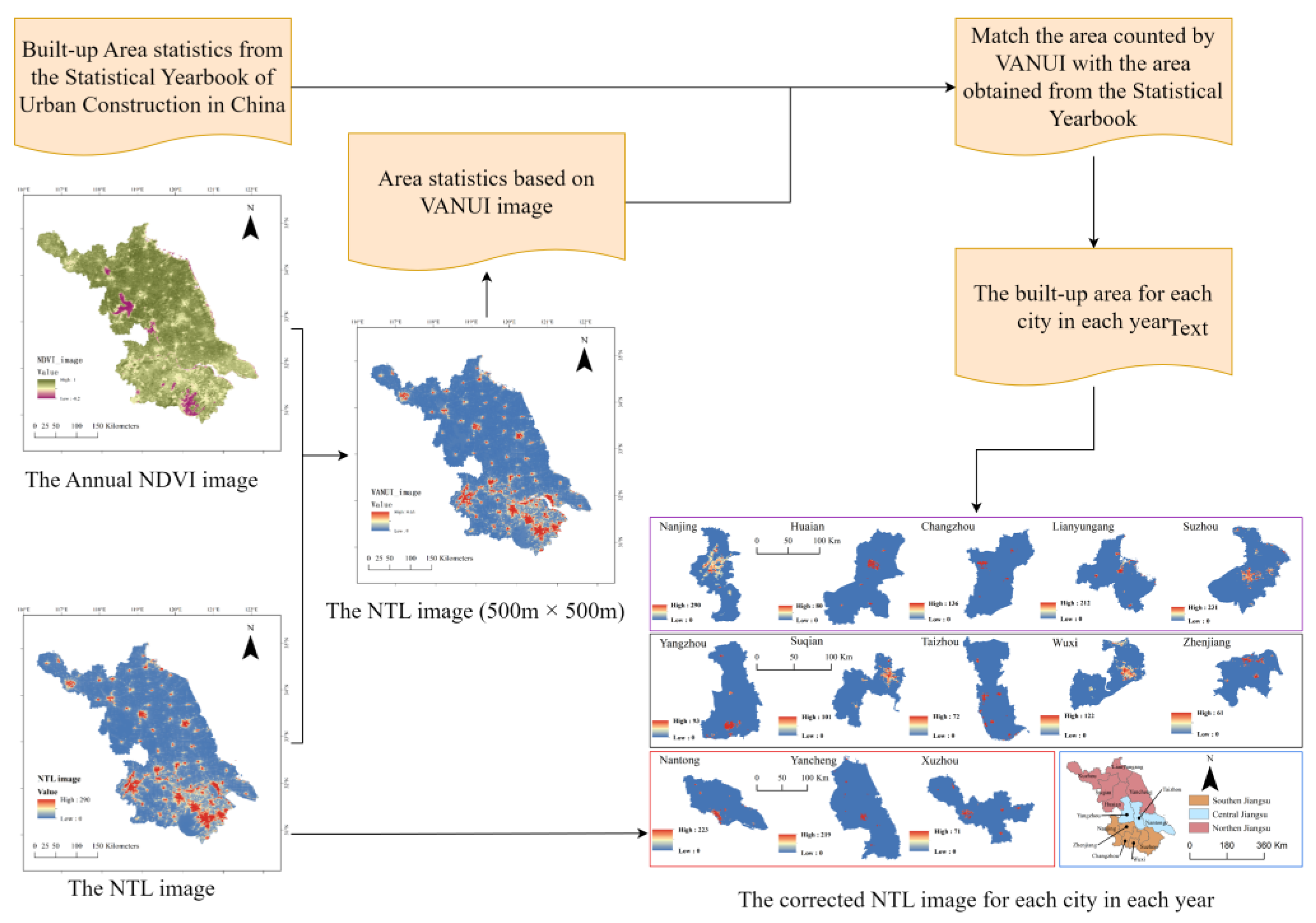
Urban energy consumption generates carbon emissions, so this study primarily focuses on urban areas. Although NTL shows a high correlation with cities, it still includes non-urban areas. To integrate ECCE with NTL, it is necessary to process the NTL data first. The specific processing flow of the NTL data is shown in Figure 2.

3.1.1. The VANUI Index to Eliminate the “Saturation Effect”

Although the NTL data has been filtered, the “saturation effect” [21] of NPP-VIIRS NTL data—where light information is displayed on the image in areas without lights on the ground—still existing. Therefore, the NTL data must be desaturated before being used. Since areas with strong night lights are often urban built-up areas, and urban areas typically have less vegetation cover, there is a negative correlation between night light data and vegetation indices. Based on this idea, Zhang et al. [22] proposed the V A N U I index, which combines N D V I data and the NTL DN values.
V A N U I = N T L n × ( 1 N D V I )
where N T L n is the normalized NTL data digital number (DN) value, and NDVI is the normalized vegetation index.

3.1.2. Extraction of Urban Built-Up Areas in NTL Data

In the above calculations, V A N U I has characteristics that are highly correlated with urban areas, meaning that the higher the value of V A N U I , the greater the likelihood of that it represents an urban area. Therefore, after completing the calibration of NTL data using V A N U I , this study extracts the built-up areas from the NTL data in conjunction with the urban built.
We first counted the area of each pixel from the highest value to the lowest value of the V A N U I calculation results each year, where the pixel size of the V A N U I image is 500 m, and accumulated the area from the highest value to the lowest value. Since the higher value part is more likely to be an urban area, the higher value is often distributed in the central area of the city, which typically has a smaller area, while the lower value is often distributed outside the city, covering a larger area. Next, we match the area accumulation value for each V A N U I threshold with the built-up area data of each city from each year’s publication in the city statistical yearbook, thereby identifying the corresponding V A N U I threshold. We then considered the part above the threshold as the urban built-up area and the part below as non-urban, thereby completing the extraction of the urban built-up area.
After obtaining the urban built-up area mask of each city in Jiangsu Province for each year, we applied this mask to the original NTL, resulting in NTL that can be used to fit the ECCE accurately.

3.2. Calculation of City Level Energy Consumption Carbon Emissions (ECCE)

The ECCE refers to the carbon emissions generated by energy use. This study, based on the calculation methods provided by the IPCC method [8,29,30,31,32], selected the 12 most important types of energy in industrial production as the foundation and used the following formula for calculation:
C O 2 = 44 12 × i = 1 12 K i E i
where C O 2 for ECCE, in units of 10,000 tons; Ki is the factor for the i-th type of energy when converted to standard coal; Ei is the the i-th type of energy consumption statistics, in units of 10,000 tons of standard coal, as shown in Table 2.

3.3. Correlation of NTL with ECCE

In this study, Total digital number of NTL data (SDN) is selected as the indicator for NTL data [28], and the Pearson correlation coefficient is utilized to determine the relationship between the NTL data and the ECCE in Jiangsu Province.
r = i = 1 n ( X i X ¯ ) ( Y i Y ¯ ) i = 1 n ( X i X ¯ ) 2 i = 1 n ( Y i Y ¯ ) 2
where the range of r is [−1,1], n is the number of sample points, which is 13 in this study, and X i and Y i are the NTL data volume SDN and ECCE of the i - t h district and county, respectively. X ¯ and Y ¯ are the mean values of the variables, respectively.

3.4. Simulation Model of Carbon Emissions from Energy Consumption Based on Night-Time Light Data

In this study, the specific idea of downscaling inversion of regional ECCE for NTL data [12,26] is as follows: We assumed that the ECCE has the similar characteristics at the county level and the city level. This is due to the fact that the development of each city in Jiangsu Province is at a high level, and the internal districts and counties should also be in the same situation of rapid development. Within each city, each district and county should have similar industrial characteristics, and the energy consumption levels are converging. Moreover, since the NTL statistics of the city are derived from the cumulative NTL of its districts and counties, the districts and counties should also have the same characteristics as the city in terms of NTL data. Therefore, we believe that the model established at the city level is also applicable at the district and county levels. Thus, after fitting a model to NTL and ECCE at the city level, the NTL of each district and county can be entered to obtain the estimated ECCE of each district and county.
Integrating existing studies [29,30], the current model for fitting the ECCE value from NTL data generally uses a simple functional regression, but the specific model varies depending on the region, which may lead to different characteristics of carbon emissions and the use of different models. To better construct a simulation model between the total intensity of NTL and ECCE in Jiangsu Province, this study selects different function models for simulation. The specified formulas for each model are shown in Table 3.

4. Analysis of Changes in Energy Consumption Carbon Emissions Based on Estimates of Nighttime Light Data

4.1. Carbon Intensity of Energy Consumption (ECCE Intensity)

To estimate the situation of ECCE in Jiangsu province, we adopted the carbon intensity of energy consumption (ECCE intensity) to figure it. ECCE intensity is a quantitative indicator of carbon emission reduction. The definition of Carbon intensity of energy consumption is shown in Formula (5), with the unit being ton per 10,000 RMB. The smaller the value, the less carbon emissions is emitted when producing the same output value.
C I = C G R P
where C I is the carbon intensity of energy consumption (ECCE intensity), C is ECCE, and G R P is Gross Regional Product.

4.2. Characterization of Time-Trends in ECCE

The characterization of the time-trend of ECCE is generally based on the S L O P E propensity value method, which uses a univariate linear regression model to calculate the S L O P E propensity value of ECCE in each district and county in different years:
S L O P E = n × i = 1 n i × C i ( i = 1 n i ) ( i = 1 n C i ) n × i = 1 n i 2 ( i = 1 n i ) 2
where n is the number of years ( n = 10), and i represents the year number, C i indicates the ECCE of each district and county in the i - t h year.
The S L O P E values are categorized into five categories: rapidly decreasing, low-speed decreasing, basically unchanged, low-growth, and rapidly growing. The categorization criteria are shown in Table 4.

4.3. Characterization of Spatial Auto-Correlation of ECCE

4.3.1. Characterization of Spatial Auto-Correlation Based on the Global Moran’s I Index

This study uses the global Moran’s I index [33] to study the global spatial auto-correlation characteristics of ECCE in Jiangsu Province. The Global Moran’s I can describe the aggregation pattern of spatial data, and it ranges from −1 to 1, with different values representing different spatial auto-correlation characteristics.
s 2 = 1 n i = 1 n ( x i x ¯ ) 2
I = i = 1 n ( x i x ¯ ) j = 1 n ( x j x ¯ ) s 2 i = 1 n j = 1 n W i j
where x i and x j represent the attribute values of districts and districts; n is the number of districts; and W i j represents the matrix of spatial weighting coefficients.
The standardized statistics Z and p values can usually test whether ECCE exhibits a random distribution in space. Here, Z is the Z score of Moran’s I index, and p represents the significance of Moran’s I index. The test criteria are shown in Table 5.

4.3.2. Characterization of Spatial Auto-Correlation Based on the Local Moran’s I Index

To further clarify the spatial characteristics of ECCE in Jiangsu Province, this study adopts the Local Moran’s I index to carry out a study on the spatial characteristics of ECCE in Jiangsu Province. The Local Moran’s I is used to identify the local spatial auto-correlation characteristics in spatial data. It helps to identify hot spots (areas where high values are clustered), cold spots (areas where low values are clustered), spatial isolates (areas where high or low values are surrounded by opposite values), and spatially homogeneous areas (areas of similar values) in spatial data [34]:
I i = n ( x i x ¯ ) j = 1 n W i j ( x j x ¯ ) i = 1 n ( x i x ¯ ) 2
where n is the number of districts and counties in Jiangsu Province, x i and x j denote the attribute values of district i and district j , and W i j denotes the spatial weight matrix. The test methods of the Local Moran’s I index and the Global Moran’s I index are the same, and both are tested by the standardized statistic Z. The criteria for the Global Moran’s I index is shown in Table 6

4.3.3. Characterization of Spatial Auto-Correlation Based on Local G i * Index

In addition to the local auto-correlation coefficient, the Local Getis–Ord G i * index can intuitively reflect the specific location of the quantitative hot spots (high values) clustering and cold spots (low values) clustering of ECCE. The Local Getis–Ord G i * statistic is a local spatial auto-correlation index for identifying hot and cold spots in spatial data. It was proposed by Arthur Getis and J. K. Ord [35] to detect the presence of statistically significant clustered regions of high or low values in a spatial distribution.
G i * = j = 1 n w i j x j j = 1 n x j
where n is the number of districts, W i j is the matrix of spatial weighting coefficients between districts i and districts j , and x j is the attribute value of district j . The Local G i * index is also examined by the standardized statistic Z. Based on the calculated Z-score and p-value, the index can be classified into the following six categories: highly significant hot spot, more significant hot spot, significant hot spot, insignificant, significant cold spot, and more significant cold spot. The criteria for their division are shown in Table 7.

5. Result

5.1. The Accounting Result of ECCE

According to the Formula (1), we used the IPCC method and finally get the result of ECCE in Jiangsu province from 2013 to 2022, as shown in Table 8.

5.2. Calculation of the Correlation between NTL Data and ECCE and Model Fitting Results

With the Formula (3), we calculated the Pearson’s r for each year, and the result are shown in the Table 9.
Table 9 shows that the Pearson’s r are all greater than 0.9, and the significance reaches six decimal places, which is about 0, much less than 0.01, and passes the two-sided test at the level of 0.01. These data indicate that the NTL data in Jiangsu Province is highly correlated with the corresponding ECCE, and the NTL data in Jiangsu Province can be used to simulate the carbon value.
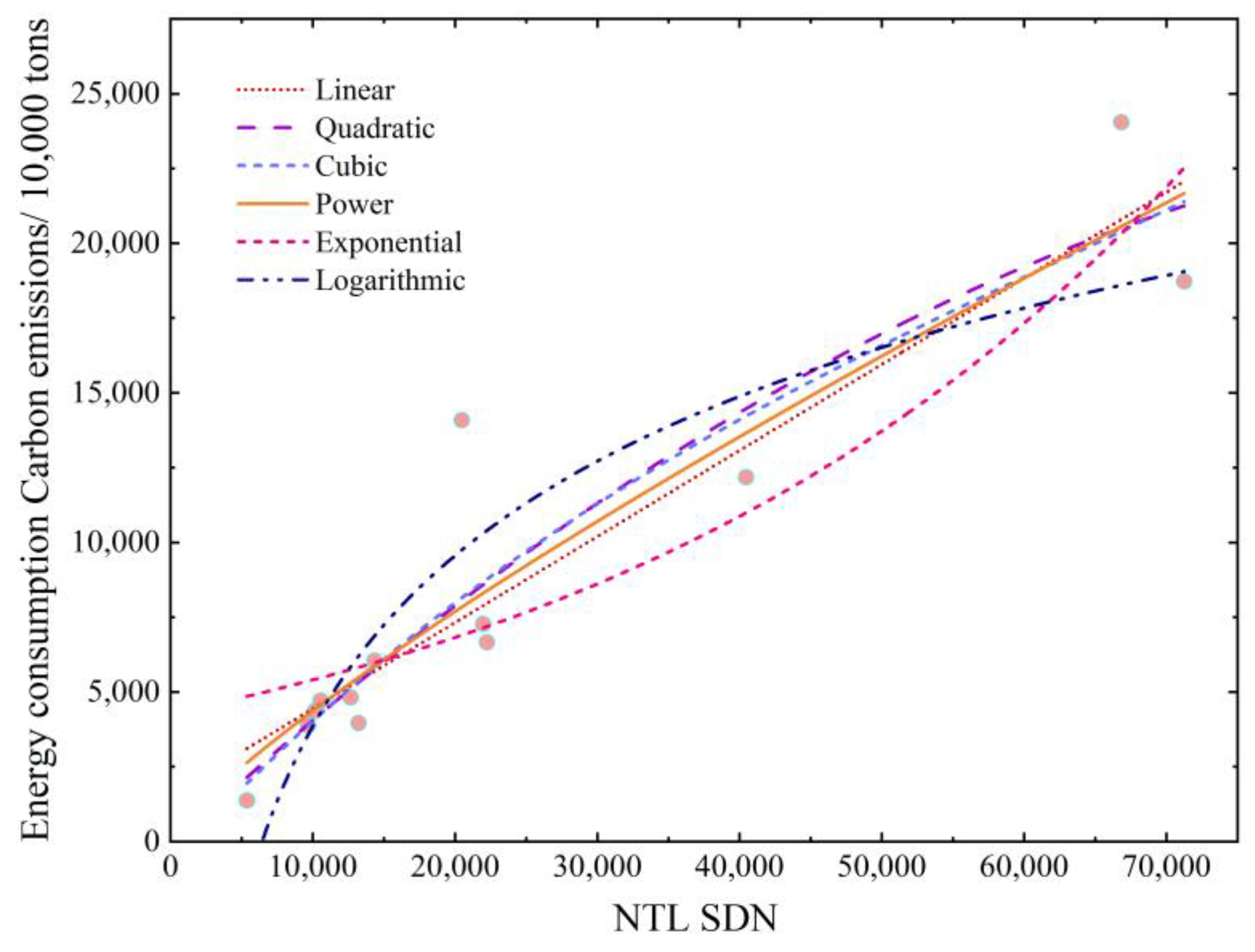
To simulate the NTL data and the ECCE, we carried out the fitting modelling for both using each function model year by year. For example, the fitted image for 2013 is shown in Figure 3, and the goodness of fit R2 values for each model are shown in Table 10.
Combining Figure 3 with Table 10 shows that, among the six models of linear—logarithmic, quadratic, cubic, power, and exponential functions—the power function has the highest R2 of 0.883, while the exponential function has the lowest R2 of 0.714. All six models have passed the significance test at the 0.001 level. The power function model is therefore chosen as the fitting model for NTL SDN data and ECCE data,
C O 2 = a × S D N b
where E C C E is the estimated ECCE, and S D N is the NTL data statistics.
By combining the city-level NTL SDN data obtained statistically for each year and the ECCE data, a functional regression was performed using a power function model, and the fitting model and R2 for each statistical year are shown in Table 11.
The R2 values were all above 0.8 during 2013–2022, which illustrates that the NTL data and ECCE have shown a very strong relationship at the city level. Based on the assumptions of this study, the fitted model obtained at the city level can be combined with the NTL values of each district and county obtained from the sub-district statistics. This allows for the estimation of the carbon emission values from energy consumption by NTL in each district and county of Jiangsu Province from 2013–2022.

5.3. Fundamental Characterization of ECCE

With the completed estimation of ECCE at country-level of Jiangsu Province, this study then analyzes the ECCE of Jiangsu Province over the decade from 2013–2022, focusing on two main aspects.

5.3.1. Fundamental Characterization of Total ECCE in Jiangsu Province

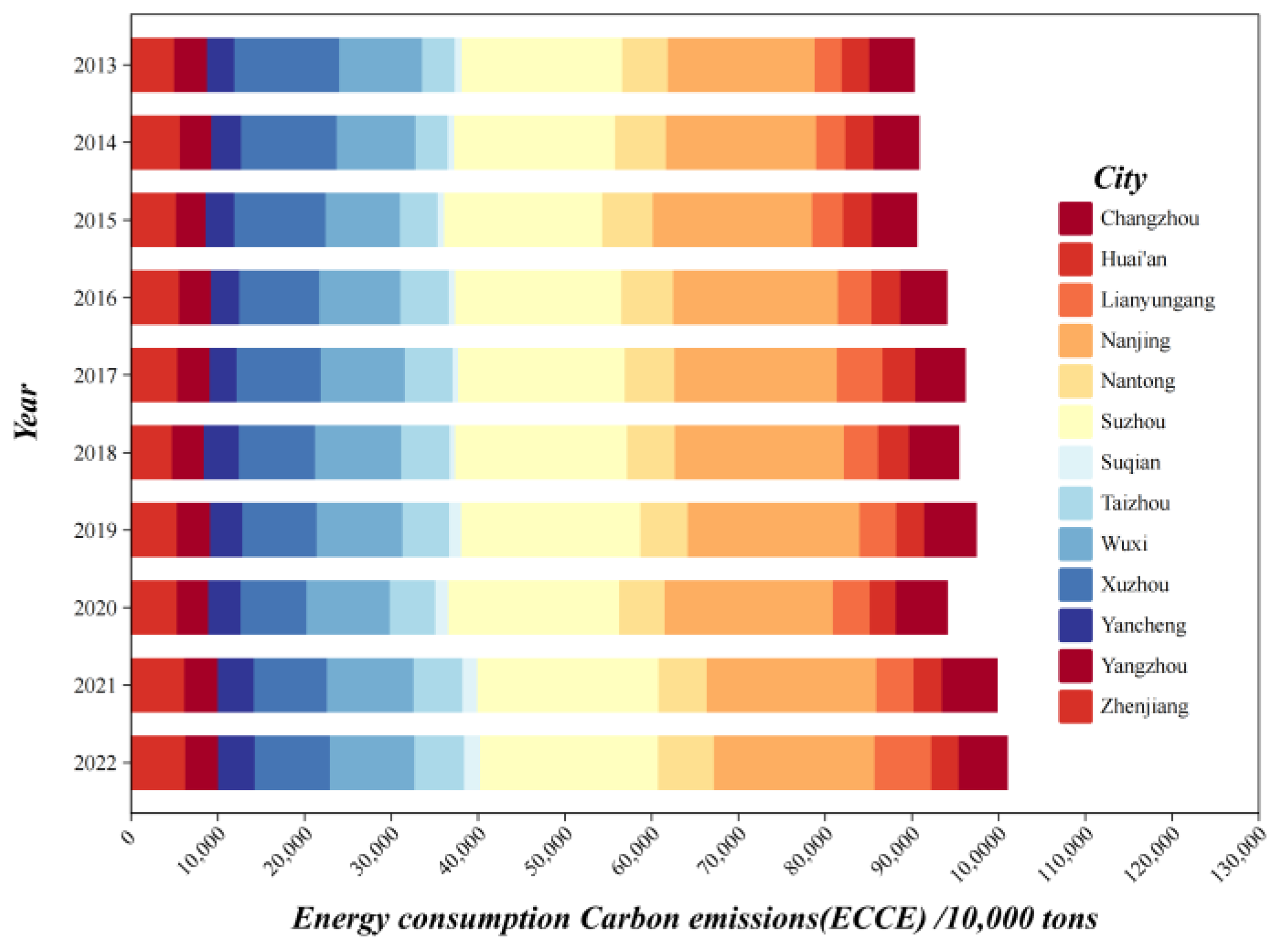
First, this study uses stacked bar charts to analyze the total characteristics of provincial and urban ECCE, and the change characteristics over 10 years, which is shown in Figure 4.
During the period from 2013 to 2022, the overall trend of ECCE in Jiangsu Province exhibited growth, decline, and then growth. This trend, when combined with the specific years, can be divided into three phases to be analyzed separately: 2013–2017 is the first phase, 2017–2020 is the second phase, and 2020–2022 is the third phase.
Within the first stage, ECCE in Jiangsu Province show a year-on-year growth trend, rising from 903.5 Mt in 2013 to 96.151 Mt in 2017. The growth rate during 2013–2015 was slower, with the change remained at 903.5 Mt to 906.18 Mt. In 2015–2017, the rapid growth stage, the change was from 906.18 Mt in 2015 to 961.51 Mt in 2017, and the growth rates were all above 2.1%. In 2016–2017, the growth rate was 3.84%. In the second phase, the change was generally on a downward trend, decreasing from 961.51 Mt in 2017 to 954.71 Mt in 2018, then slightly rising to 974.59 Mt in 2019, and then decreasing to 941.4 Mt in 2020. In the third stage, ECCE in Jiangsu Province were on the rise again, from 941.4 Mt in 2020 to 998.54 Mt in 2021 and 1010.33 Mt in 2022, with a faster growth rate in 2021.
This study visualizes the spatial distribution of ECCE in each county of Jiangsu Province through the spatial map as shown in Figure 5. The changes in ECCE of each city in Jiangsu Province are different, and large differences arise in ECCE between cities. Among these cities, Xuzhou shows a clear downward trend; Zhenjiang, Yangzhou, Huaian, and Nantong basically remain unchanged; and Yancheng, Wuxi, Taizhou, Suqian, Suzhou, Nanjing, Lianyungang, and Changzhou show an increasing trend. Among the cities, Xuzhou, Nanjing, Suzhou, Wuxi, and Changzhou, which are higher-carbon emission cities, have ECCE levels above 70 Mt. In contrast, Zhenjiang, Yangzhou, Huaian, Nantong, Yancheng, Taizhou, Suqian, and Lianyungang, which are lower-carbon emission cities, have ECCE levels below 70 Mt.
According to Figure 5, the southern region of Jiangsu Province has the highest levels of ECCE, while the northern and central regions have the lowest levels. The primary concentration areas with higher values are Nanjing and Suzhou. In addition, the cities between Nanjing and Suzhou also maintain higher levels of ECCE. Over the 10-year period, ECCE in some districts and counties has increased from 10–20 Mt to 20–30 Mt. Findings from Northern Jiangsu indicate that ECCE in several districts and counties increased from less than 5 Mt to between 5–10 Mt. During the period from 2013 to 2022, the development of cities in North Jiangsu brought about a significant increase in the cities’ ECCE. The central part of Jiangsu Province is the main distribution area of lower ECCE values.

5.3.2. Characterization of ECCE Intensity in Jiangsu Province

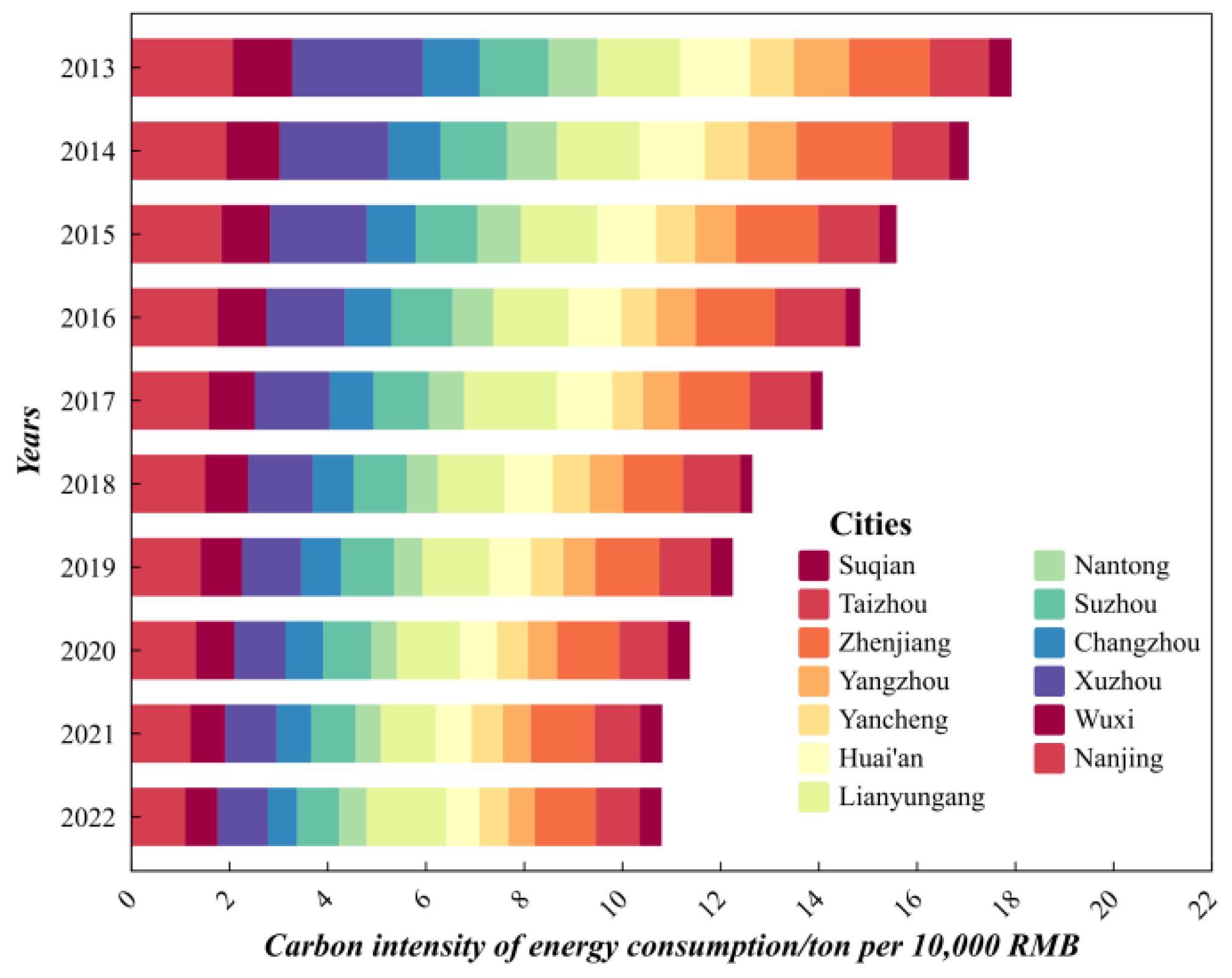
Using Formula (4), this study calculates and describes ECCE intensity at provincial and urban levels in Jiangsu Province from 2013 to 2022. The results are visualized using stacked bar charts, as shown in Figure 6.
During the period from 2013 to 2022, the ECCE intensity in Jiangsu Province showed a year-by-year decline, indicating that the amount of ECCE produced per unit of output decreased over time, improving economic efficiency. The ECCE intensity dropped from 1.55 tons/million RMB in 2013 to 0.82 tons/million RMB in 2022. Among these improvements, the growth rate in 2015 has the largest change, amounting to −9.29%. The analysis shows that the ECCE intensity of each city in Jiangsu Province also followed a year-on-year decreasing trend, with Xuzhou City experiencing the largest change in the ECCE intensity, dropping from 2.65 tons/million RMB in 2013 to 1.02 tons/million RMB in 2022. In general, Nanjing, Xuzhou, Zhenjiang, and Lianyungang are the cities with the highest ECCE intensity, followed by Wuxi, Changzhou, Suzhou, Huaian, and Taizhou. Finally, Nantong, Yancheng, Yangzhou, and Suqian have the lowest ECCE intensity.

5.4. Results of Temporal Variation Analyses

Combined with the measured ECCE of each county in Jiangsu Province, the S L O P E tendency values of each county were calculated according to the Formula (5), and the S L O P E tendency spatial distribution of the ECCE of the counties in Jiangsu Province is shown in Figure 7.
Seven districts and counties in Jiangsu Province are in a rapid rate of decrease, thirteen districts and counties are in a low rate of decrease, sixty-one districts and counties are basically unchanged, seven districts and counties are in a low rate of increase, and seven districts and counties are in a rapid rate of increase. The specific types of changes of the 95 districts and counties are shown in Table 12. In Jiangsu Province, most districts and counties were in a relatively stable state in the decade 2013–2022. Some districts and counties show a decline, mainly due to industrial structure adjustment and energy structure changes. Examples include Tongshan District in Xuzhou City, Huqiu District in Suzhou City, and Xinwu District. Some districts and counties in the urban area show growth, mainly due to urban expansion and industrial development, such as Jiangning District in Nanjing City, Pukou District, Wuzhong District in Suzhou City, and Xiangcheng District.

5.5. Results of Spatial Variation Analyses

5.5.1. Results of the Global Moran’s I Index

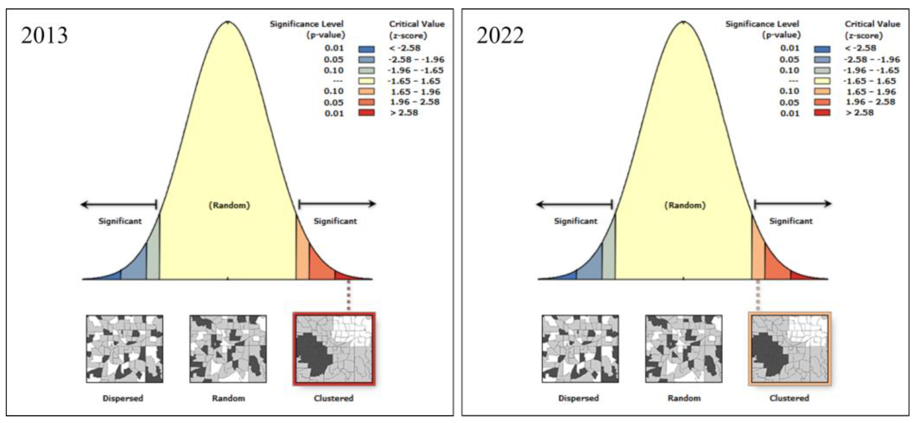
Using the Formulas (6) and (7), the results of calculating the spatial auto-correlation of ECCE in Jiangsu Province from 2013 to 2022, for example, in 2013 and 2022, are shown in Figure 8. The Moran’s I score, Z score, and corresponding p value calculated for the spatial distribution of county-level ECCE in Jiangsu Province in 2013 and 2022 are shown. The figure also gives the spatial clustering types classified according to the different Z scores and Z scores corresponding to the p value. Here, blue shows discrete, while red shows clustering, with the darker the color, the more obvious the corresponding clustering characteristics. Yellow indicates no obvious spatial aggregation performance, meaning the distribution of spatial data is random. In addition, Figure 8 gives the corresponding positions of the computed results of the year on the p-value distribution, with the right side showing aggregation, the left side showing discrete, and the center showing random distribution. Based on the calculation results of 2013 and 2022, the spatial characteristics of county-level ECCE data of Jiangsu Province in 2013 and 2022 show aggregation, while 2013 is represented by dark red and 2022 is represented by light red, indicating that the ECCE of Jiangsu Province in 2013 were more spatially aggregated.
Statistics of global Moran’s I index, Z-score, and p-value calculations of ECCE in Jiangsu Province from 2013 to 2022 are shown in Table 13.
The combination of Table 5 and Table 13 shows that the global Moran’s I index of ECCE in Jiangsu Province are all positive, that is, the total amount of ECCE in Jiangsu Province has a significant positive spatial correlation. Except for the year 2020, the distribution of ECCE in Jiangsu Province shows more obvious aggregation characteristics. The confidence level of 2021 and 2022 is 90%, the confidence level of 2017, 2018 and 2019 is 95%, and the confidence level of 2013, 2014, 2015 and 2016 is 99%. These results allow us to infer that the global Moran’s I index of ECCE in Jiangsu Province is currently showing a decreasing trend in time series, i.e., the spatial distribution of ECCE in Jiangsu Province shows a phenomenon of flat proximity.

5.5.2. Results of the Local Moran’s I Index

The calculation results in Figure 9, combined with the classification criteria in Table 6, clearly show that the Local Moran’s I index in Jiangsu Province over the ten-year period is mainly characterized by high-high clustering in Nanjing and Suzhou, which rank first and second in Jiangsu Provinces GDP, respectively. The development of these two cities is more complete, and their industries are more developed, resulting in higher energy consumption and carbon emissions within these cities compared with the rest of the province, thereby exhibiting a high-high clustering phenomenon. By contrast, the main urban areas of Nantong in some years, specifically within 2016, 2017, 2018, 2020, and 2021, as well as the main urban areas of Huai’an within 2013, 2014, and 2015, show a high–low clustering characteristic, mainly due to the slower development of these cities. Here, the main urban areas develop faster than the neighboring districts and counties. Thus, the main urban areas cause the ECCE to be higher than those of the neighborhood, resulting in a high–low clustering characteristic.

5.5.3. Results of the Local G i * Index

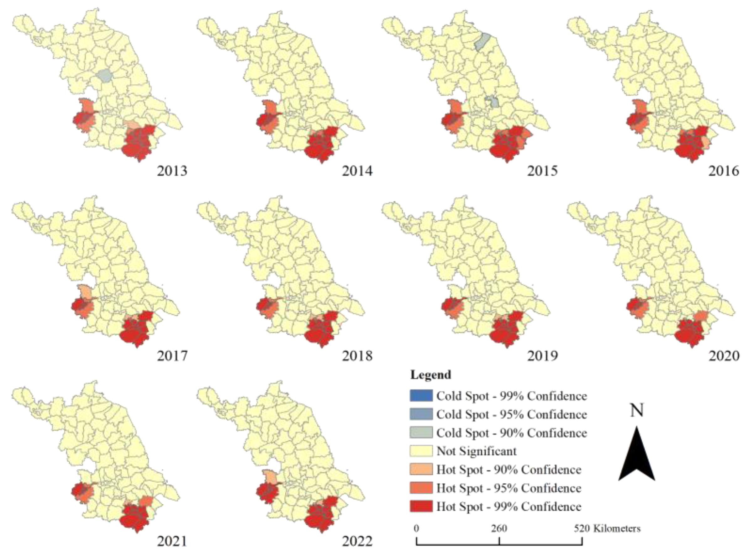
Formula (9) is combined with Table 7, and the results of calculating the Local Getis–Ord G i * index of county-level ECCE in Jiangsu Province for each year from 2013–2022 are shown in Figure 10.
In 2013–2022, ECCE in Jiangsu Province generally shows a hot spot phenomenon in Nanjing and Suzhou. The main city of Wuxi, which is close to Suzhou, also shows a hot spot phenomenon. In general, the high values of ECCE in Jiangsu Province are aggregated in the southern part of Suzhou. In some years, cold spots are found in the north and center of Suzhou, but none of them are extremely significant cold spots. Overall, ECCE in Jiangsu Province are higher in the south and low in the north, consistent with the current situation of urban development and urban GDP.

6. Discussion

6.1. Reliability Validation of Estimating ECCE Based on NTL Data

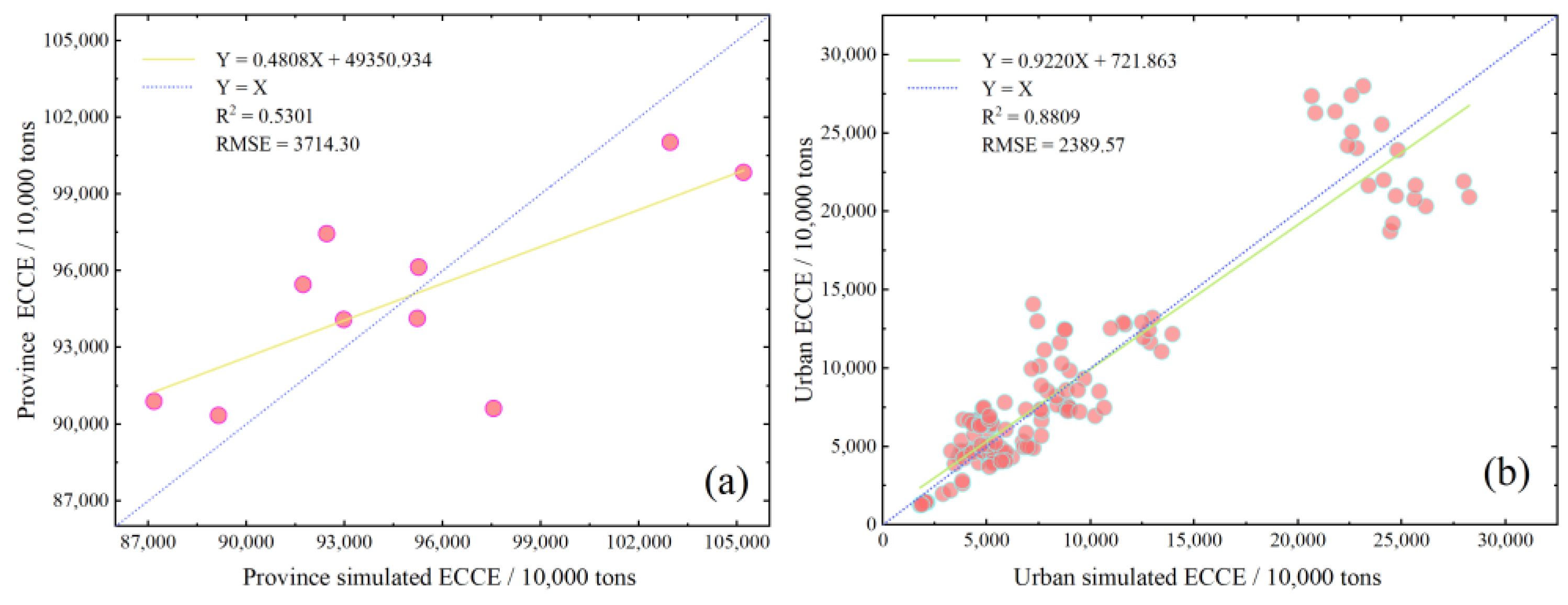
The method of estimating ECCE from NTL data adopts a functional regression. In this study, to avoid spurious regression, an error analysis was carried out at the provincial and urban levels to validate the regression results [36], i.e., by adding up the estimated county-level ECCE according to the city they belong to, we get the estimated value at urban and provincial levels. Given that the urban and provincial ECCE data were obtained through the IPCC method of statistics, which is widely accepted, this study adopted the linear regression and table analysis to verify the reliability, as shown in Table 14 and Figure 11. The horizontal coordinate is the fitting simulation value, and the vertical coordinate is the IPCC accounting value.
Figure 11 shows that the R2 of the 2013–2022 NTL data to estimate ECCE in the linear regression at the provincial level is 0.53, and the R2 at the city level scale is 0.88, which is within the acceptable range. The provincial errors specific to the year are shown in Table 14, and this study chooses the relative error RE.
The carbon emission results fitted by each district and county are accumulated to obtain the simulated carbon emissions values of Jiangsu Province in each year from 2013 to 2022, and the relative errors are calculated as shown in the table. During the 10-year period from 2013 to 2022, the smallest relative error is in 2021, −0.19%, and the largest is in 2016, −7.03%. The absolute value of the relative errors during the 10-year period is less than 10%, showing that the fitting results are similar to the IPCC measurement results, and the errors are within reasonable limits.

6.2. Spatiotemporal Patterns of Energy Consumption Carbon Emissions in Jiangsu Province

In this study, our results show the same trend based on the comparison of the data published in Scientific Data by Chen et al. [36]. for the estimation of ECCE in Chinese cities up to 2019. ECCE in Jiangsu province shows a fluctuating upward trend during 2013–2022, which is mainly divided into three stages: a gradual increase from 2013–2017, a fluctuating decrease from 2017–2020, and a gradual increase from 2020–2022. The faster growth before 2017 is mainly considered urban development and economic growth, which led to a large amount of industrial ECCE. Combined with the socio-economic data of Jiangsu Province, the GDP growth rate of Jiangsu Province in 2016–2017 was 11.01%, and the growth rate of its industrial output was 11.53%, indicating rapid development. While urban growth slowed down during 2017–2020, Jiangsu Province has implemented the ‘13th Five-Year Plan’ comprehensive energy conservation and emission reduction policy, mainly optimizing the energy structure and industrial structure. In addition, considering the impact of the epidemic, the slowdown of industrial production within this period led to the decline of ECCE in 2020. From 2020 to 2022, ECCE increased again due to the resumption of industrial production, which led to a renewed increase in industrial consumption.
ECCE in all districts and counties show different degrees of change, and the districts and counties with higher ECCE are unevenly distributed in Jiangsu Province, mainly concentrated in the southern cities of Jiangsu Province, such as Jiangning District in Nanjing and Xiangcheng District and Huqiu District in Suzhou, which is similar to the results of the study by Meng et al. [37]. These districts are mostly the core areas of urban development, so the focus of energy conservation and emission reduction efforts is more on the development of built-up areas. In terms of the time S L O P E trend of ECCE in districts and counties, Tongshan and Quanshan districts in Xuzhou show a decreasing trend, and in combination with the change of energy consumption in Xuzhou, it can be found that the use of high-emission energy sources, such as raw coal and coke, is significantly reduced in Xuzhou. In all regions of Jiangsu Province, areas with slowly increasing ECCE are distributed, such as the Jianye district area in Nanjing, the Runzhou district in Zhenjiang, and the Pizhou district in Xuzhou, which are distributed in the middle and outer periphery of the city, as a result of urban expansion. In order to achieve the effect of energy saving and emission reduction, it is not only necessary to pay attention to the city centers, but also to focus on the newly developed areas and control the use of high-emission energy sources.

6.3. The Policy Suggestion for Energy Conservation and Emission Reduction

From the results of the study, although the ECCE of Jiangsu Province shows a fluctuating increase, its ECCE intensity has been decreasing year by year, and Jiangsu Province has not yet reached the peak of carbon emission. Therefore, policymakers need to continue to strengthen the control of ECCE during economic development and further increase the ECCE intensity, in order to achieve economic growth while saving energy and reducing emissions as much as possible [38]. In terms of distribution, urban centers are the main concentration of high ECCE, and policies should restrict them, such as limiting energy consumption in urban centers and relocating high-energy-consuming and high-emission enterprises. In addition, Jiangsu Province shows obvious regional inequality in ECCE, with ECCE in the southern part of the province significantly higher than in the central and northern parts. To strengthen the exchange of ECCE across the province, more developed cities in southern Jiangsu, such as Nanjing and Suzhou, should make full use of their developed economis to adjust their focus of development to a low-carbon economy, and pay attention to the development of low-carbon technologies. Central and northern Jiangsu, which are relatively underdeveloped, should actively adjust their energy structure and use cleaner energy while maintaining development, minimizing the use of high-emission energy sources, as seen in Xuzhou. Technological exchanges should be strengthened within Jiangsu Province, with southern counties and cities transferring low-carbon talent and methods to central and northern Jiangsu to promote integrated development and achieve the “dual-carbon target” as soon as possible.

6.4. Limitations

Although NTL data have been widely used and recognized in estimating carbon emissions, using NTL data as a single variable to invert ECCE is not comprehensive. The influencing factors of regional ECCE may also include industrial structure, urban population, and energy structure. However, the current use of NTL data does not take these multiple variables into account. Thus, the estimated values by using NTL data may fluctuate greatly. Second, the relationship between NTL data and ECCE can be complex. On the one hand, NTL data reflects the value of city lights at night rather than directly showing the daytime industrial situation in the city. Most current research uses a simple regression model to represent the relationship between NTL data and ECCE data. With the development of machine learning and deep learning, combining multiple factors and machine learning techniques may be necessary to construct a deeper and more scientific model for estimating. On the other hand, the estimation should take a multi-source data approach in the future. With the development of NTL data, such as the launch of the LuoJia 1-01 satellite [39], higher resolution NTL data can be obtained, potentially improving the accuracy of the estimation. This data should be combined with other auxiliary data, such as Landsat satellite data, POI data, and road network data, to improve the accuracy of the estimation.

7. Conclusions

This study chose to utilize the NPP VIIRS nightlight time (NTL) data, and combined it with the IPCC ‘inventory method’, to estimate and analyze the spatiotemporal changes in energy consumption carbon emissions (ECCE) at the district and county scales. The conclusions from the study of Jiangsu Province from 2013–2022 are as follows:
The ECCE in Jiangsu Province shows a fluctuating upward trend, and it mainly shows three phases during the 10-year period: a gradual rise from 2013–2017, a fluctuating decline from 2017–2020, and a gradual increase from 2020–2022. By analyzing the ECCE intensity, it can be observed that although ECCE in Jiangsu Province shows fluctuations during the period of 2013–2022, the ECCE intensity shows a year-on-year decrease.
In the time dimension, ECCE from districts and counties were classified into five classes, and from 2013–2022, the districts and counties showed different degrees of changes in ECCE, with a number of districts and counties increasing from less than 5 Mt to 5–10 Mt grades. Through the S L O P E analysis, most of the districts and counties (a total of 61) showed that the ECCE basically remained unchanged, seven districts and counties showed a decreasing trend, seven districts and counties rose slowly, and seven districts and counties rose rapidly. Most of the districts and counties with rapidly rising ECCE were located in the main urban areas of the city.
In the spatial dimension analysis, it was found that the districts and counties in the southern part of Jiangsu Province produced significantly more ECCE than those in the central and northern parts of the province. By using global Moran’s I index, it was found that ECCE at the district and county levels in Jiangsu Province showed obvious spatial clustering characteristics. With the Local Moran’s I and the Local G i * index, it was found that in the southern part of Jiangsu Province, the hot spots were in Nanjing and Suzhou City, which showed high-high clustering.

Author Contributions

The study was completed with cooperation between all authors. C.X. and Y.M. designed the research topic; Y.M. conducted the experiment; C.X. and A.L. checked and analyzed the experimental results; C.X. and Y.M. wrote the paper. All authors have read and agreed to the published version of the manuscript.

Funding

This research was funded in part by the Natural Science Foundation of Jiangsu Province, China under Grants BK20180809; in part by the National Natural Science Foundation of China under Grants 41901274; in part by the Talent Launch Fund of Nanjing University of Information Science and Technology under Grant 2017r066.

Data Availability Statement

The data used in this study are all open. The VIIRS NTL data is derived from the Earth Observation Group, which links to https://eogdata.mines.edu/products/vnl/ (accessed on 17 September 2024). The Annual Normalized Difference Vegetation Index (NDVI) data is derived from the https://search.earthdata.nasa.gov/search (accessed on 17 September 2024). The statistical data of Jiangsu province is derived from the Statistical Yearbook of Urban construction in China and Statistical Yearbook of Jiangsu Province.

Conflicts of Interest

The authors declare no conflicts of interest.

References

  1. Wei, Y.; Wang, L.; Liao, H.; Wang, K.; Murty, T.; Yan, J. Responsibility accounting in carbon allocation: A global perspective. Appl. Energy 2014, 130, 122–133. [Google Scholar] [CrossRef]
  2. Lu, H.; Liu, G. Spatial effects of carbon dioxide emissions from residential energy consumption: A county-level study using enhanced nocturnal lighting. Appl. Energy 2014, 131, 297–306. [Google Scholar] [CrossRef]
  3. Qiu, R.; Han, G.; Li, X.; Xiao, J.; Liu, J.; Wang, S.; Li, S.; Gong, W. Contrasting responses of relationship between solar-induced fluorescence and gross primary production to drought across aridity gradients. Remote Sens. Environ. 2024, 302, 113984. [Google Scholar] [CrossRef]
  4. Al-Ghussain, L. Global warming: Review on driving forces and mitigation. Environ. Prog. Sustain. 2019, 38, 13–21. [Google Scholar] [CrossRef]
  5. He, C.; Ma, Q.; Li, T.; Yang, Y.; Liu, Z. Spatiotemporal dynamics of electric power consumption in Chinese Mainland from 1995 to 2008 modeled using DMSP/OLS stable nighttime lights data. J. Geogr. Sci. 2012, 22, 125–136. [Google Scholar] [CrossRef]
  6. Cheng, Y.; Wang, Z.; Ye, X.; Wei, Y.D. Spatiotemporal dynamics of carbon intensity from energy consumption in China. J. Geogr. Sci. 2014, 24, 631–650. [Google Scholar] [CrossRef]
  7. Wang, N.; Chang, Y.-C. The development of policy instruments in supporting low-carbon governance in China. Renew. Sust. Energ. Rev. 2014, 35, 126–135. [Google Scholar] [CrossRef]
  8. Fang, J.; Yu, G.; Liu, L.; Hu, S.; Chapin, F.S., III. Climate change, human impacts, and carbon sequestration in China. Proc. Nat. Acad. Sci. USA 2018, 115, 4015–4020. [Google Scholar] [CrossRef]
  9. IPCC. Climate Change 2013: The Physical Science Basis: Working Group I Contribution to the Fifth Assessment Report of the Intergovernmental Panel on Climate Change; Cambridge University Press: New York, NY, USA, 2014. [Google Scholar] [CrossRef]
  10. Liu, Y.; Wang, F.; Zheng, J. Estimation of Greenhouse Gas Emissions from the EU, US, China, and India up to 2060 in Comparison with Their Pledges under the Paris Agreement. Sustainability 2017, 9, 1587. [Google Scholar] [CrossRef]
  11. Wang, X.; Chen, Y.; Chen, X.; He, R.; Guan, Y.; Gu, Y.; Chen, Y. Crop Production Pushes up Greenhouse Gases Emissions in China: Evidence from Carbon Footprint Analysis Based on National Statistics Data. Sustainability 2019, 11, 4931. [Google Scholar] [CrossRef]
  12. Wang, Z.; Zhou, K.; Fan, J.; Zhao, H. Progress of research on energy-related carbon emission accounting methods at the prefectural and county levels. Prog. Geogr. 2023, 42, 1406–1419. [Google Scholar] [CrossRef]
  13. Wu, Q.; Gu, S. Discerning drivers and future reduction paths of energy-related CO2 emissions in China: Combining EKC with three-layer LMDI. Environ. Sci. Pollut. Res. 2021, 28, 36611–36625. [Google Scholar] [CrossRef]
  14. Zhang, Y.; Yu, Z.; Zhang, J. Analysis of carbon emission performance and regional differences in Chinas eight economic regions: Based on the super-efficiency SBM model and the Theil index. PLoS ONE 2021, 16, e0250994. [Google Scholar] [CrossRef]
  15. Han, G.; Huang, Y.; Shi, T.; Zhang, H.; Li, S.; Zhang, H.; Chen, W.; Liu, J.; Gong, W. Quantifying CO2 emissions of power plants with Aerosols and Carbon Dioxide Lidar onboard DQ-1. Remote Sens. Environ. 2024, 313, 114368. [Google Scholar] [CrossRef]
  16. Liu, B.; Ma, X.; Guo, J.; Wen, R.; Li, H.; Jin, S.; Ma, Y.; Guo, X.; Gong, W. Extending the wind profile beyond the surface layer by combining physical and machine learning approaches. Atmos. Chem. Phys. 2024, 24, 4047–4063. [Google Scholar] [CrossRef]
  17. Han, G.; Pei, Z.; Shi, T.; Mao, H.; Li, S.; Mao, F.; Ma, X.; Zhang, X.; Gong, W. Unveiling Unprecedented Methane Hotspots in China’s Leading Coal Production Hub: A Satellite Mapping Revelation. Geophys. Res. Lett. 2024, 51, e2024GL109065. [Google Scholar] [CrossRef]
  18. Elvidge, C.D.; Ziskin, D.; Baugh, K.E.; Tuttle, B.T.; Ghosh, T.; Pack, D.W.; Erwin, E.H.; Zhizhin, M. A Fifteen Year Record of Global Natural Gas Flaring Derived from Satellite Data. Energies 2009, 2, 595–622. [Google Scholar] [CrossRef]
  19. Ma, T.; Zhou, C.; Pei, T.; Haynie, S.; Fan, J. Quantitative estimation of urbanization dynamics using time series of DMSP/OLS nighttime light data: A comparative case study from China’s cities. Remote Sens. Environ. 2012, 124, 99–107. [Google Scholar] [CrossRef]
  20. Chen, Z.; Yu, B.; Song, W.; Liu, H.; Wu, Q.; Shi, K.; Wu, J. A new approach for detecting urban centers and their spatial structure with nighttime light remote sensing. IEEE Trans. Geosci. Remote Sens. 2017, 55, 6305–6319. [Google Scholar] [CrossRef]
  21. Zhuo, L.; Zheng, J.; Zhang, X.; Li, J.; Liu, L. An improved method of night-time light saturation reduction based on EVI. Int. J. Remote Sens. 2015, 36, 4114–4130. [Google Scholar] [CrossRef]
  22. Zhang, Q.; Schaaf, C.; Seto, K.C. The Vegetation Adjusted NTL Urban Index: A new approach to reduce saturation and increase variation in nighttime luminosity. Remote Sens. Environ. 2013, 129, 32–41. [Google Scholar] [CrossRef]
  23. He, C.; Liu, Z.; Tian, J.; Ma, Q. Urban expansion dynamics and natural habitat loss in China: A multiscale landscape perspective. Glob. Chang. Biol. 2014, 20, 2886–2902. [Google Scholar] [CrossRef] [PubMed]
  24. Xu, M.; He, C.; Liu, Z.; Dou, Y. How did urban land expand in China between 1992 and 2015? A multi-scale landscape analysis. PLoS ONE 2016, 11, e0154839. [Google Scholar] [CrossRef] [PubMed]
  25. Jean, N.; Burke, M.; Xie, M.; Davis, W.M.; Lobell, D.B.; Ermon, S. Combining satellite imagery and machine learning to predict poverty. Science 2016, 353, 790–794. [Google Scholar] [CrossRef]
  26. Li, C.; Jia, J.; Wu, F.; Zuo, L.; Cui, X. County-level intensity of carbon emissions from crop farming in China during 2000–2019. Sci. Data 2024, 11, 457. [Google Scholar] [CrossRef] [PubMed]
  27. Chen, J.; Li, P.; Gao, J. Spatiotemporal patterns and influencing factors of carbon emissions in the Pan-Yangtze River Delta region, 1990–2014. Prog. Geogr. 2016, 12, 1472–1482. [Google Scholar] [CrossRef]
  28. Ou, J.; Liu, X.; Wang, S.; Xie, R.; Li, X. Investigating the differentiated impacts of socioeconomic factors and urban forms on CO2 emissions: Empirical evidence from Chinese cities of different developmental levels. J. Clean. Prod. 2019, 226, 601–614. [Google Scholar] [CrossRef]
  29. Su, Y.; Chen, X.; Ye, Y.; Wu, Q.; Zhang, H.; Huang, N.; Kuang, Y. The characteristics and mechanisms of carbon emissions from energy consumption in China using DMSP/OLS night light imageries. Acta Geogr. Sin. 2013, 68, 1513–1526. [Google Scholar] [CrossRef]
  30. Zhou, S.; Wei, L.; Lu, Z.; Lu, Z. A technical framework for integrating carbon emission peaking factors into the industrial green transformation planning of a city cluster in China. J. Clean. Prod. 2022, 344, 131091. [Google Scholar] [CrossRef]
  31. Zhu, K.; Tu, M.; Li, Y. Did Polycentric and Compact Structure Reduce Carbon Emissions? A Spatial Panel Data Analysis of 286 Chinese Cities from 2002 to 2019. Land 2022, 11, 185. [Google Scholar] [CrossRef]
  32. Li, L.; Shan, Y.L.; Lei, Y.L.; Wu, S.M.; Yu, X.; Lin, X.Y.; Chen, Y.P. Decoupling of economic growth and emissions in China’s cities: A case study of the Central Plains urban agglomeration. Appl. Energy 2019, 244, 36–45. [Google Scholar] [CrossRef]
  33. Moran, P.A.P. Notes on Continuous Stochastic Phenomena. Biometrika 1950, 37, 17–23. [Google Scholar] [CrossRef] [PubMed]
  34. Li, M.; Cui, M.; Levinson, D. Interaction between Development Intensity: An Evaluation of Alternative Spatial Weight Matrices. Urban Sci. 2023, 7, 22. [Google Scholar] [CrossRef]
  35. Getis, A.; Ord, J.K. The Analysis of Spatial Association by Use of Distance Statistics. Geogr. Anal. 1992, 24, 189–206. [Google Scholar] [CrossRef]
  36. Chen, J.; Gao, M.; Cheng, S.; Hou, W.; Song, M.; Liu, X.; Liu, Y.; Shan, Y. County-level CO2 emissions and sequestration in China during 1997–2017. Sci. Data 2020, 7, 391. [Google Scholar] [CrossRef]
  37. Meng, H.; Zhang, X.; Du, X.; Du, K. Spatiotemporal Heterogeneity of the Characteristics and Influencing Factors of Energy-Consumption-Related Carbon Emissions in Jiangsu Province Based on DMSP-OLS and NPP-VIIRS. Land 2023, 12, 1369. [Google Scholar] [CrossRef]
  38. Li, M.; Liu, H.; Yu, S.; Wang, J.; Miao, Y.; Wang, C. Estimating the Decoupling between Net Carbon Emissions and Construction Land and Its Driving Factors: Evidence from Shandong Province, China. Int. J. Environ. Res. Public Health 2022, 19, 8910. [Google Scholar] [CrossRef]
  39. Cui, Y.; Zha, H.; Jiang, L.; Zhang, M.; Shi, K. Luojia 1–01 Data Outperform Suomi-NPP VIIRS Data in Estimating CO2 Emissions in the Service, Industrial, and Urban Residential Sectors. IEEE Geosci. Remote Sens. Lett. 2023, 20, 3000905. [Google Scholar] [CrossRef]
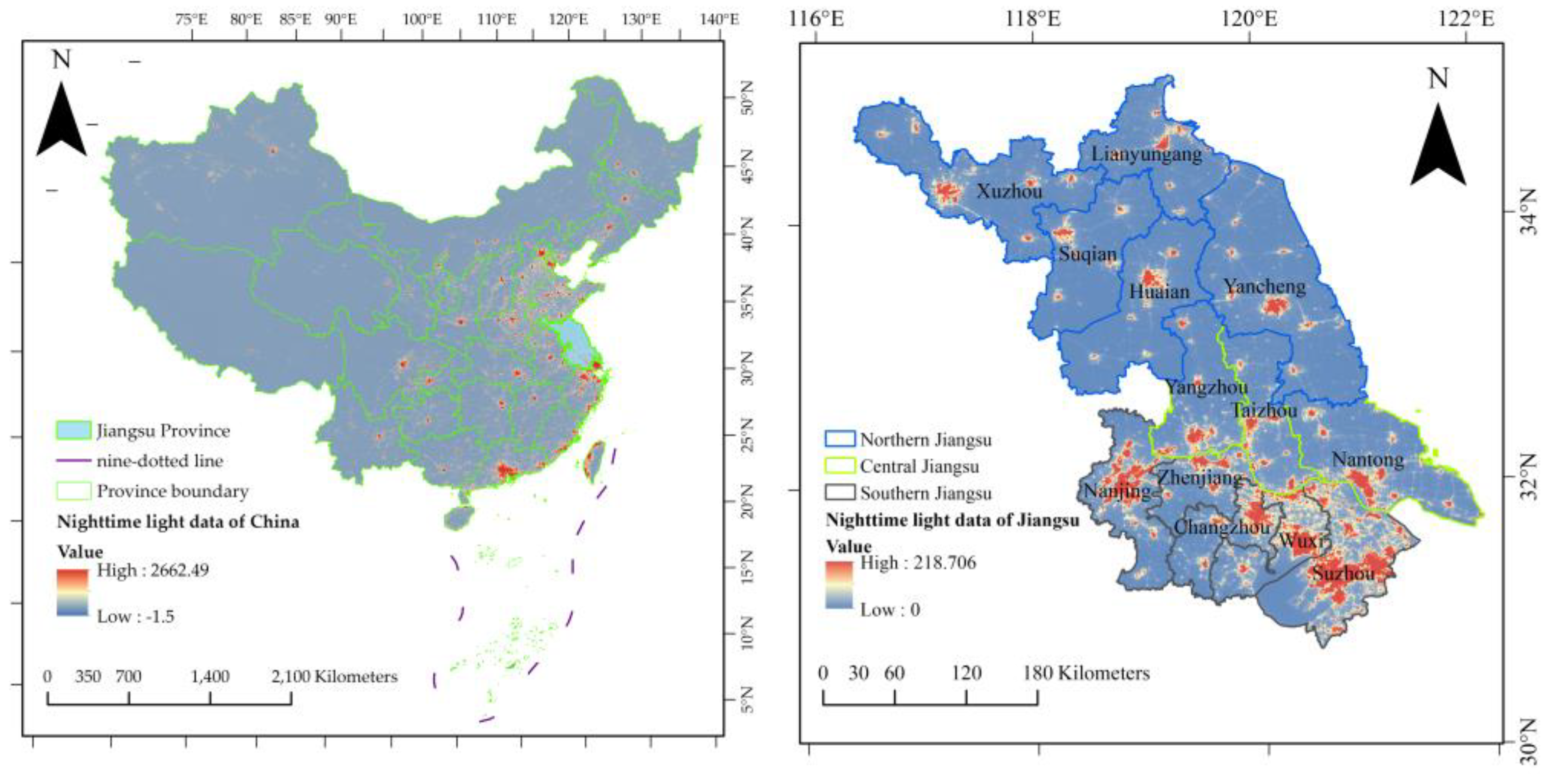
Figure 1. Distribution of NTL images and the administrative divisions and city distribution of Jiangsu Province.
Remotesensing 16 03514 g001
Figure 2. The processing flow of the NTL data. The figure uses the 2022 data as an example and calculates the corrected NTL data for each city in Jiangsu Province in 2022.
Remotesensing 16 03514 g002
Figure 3. Fitting model of NTL SDN data and ECCE data in Jiangsu Province, 2013.
Remotesensing 16 03514 g003
Figure 4. Stacked histogram of ECCE stacks in Jiangsu Province, 2013–2022.
Remotesensing 16 03514 g004
Figure 5. Spatialization of ECCE in counties of Jiangsu Province, 2013–2022.
Remotesensing 16 03514 g005
Figure 6. Stacked histogram of ECCE intensity in Jiangsu Province, 2013–2022.
Remotesensing 16 03514 g006
Figure 7. Spatial distribution of time-trend characteristics of ECCE at county-level in Jiangsu Province.
Remotesensing 16 03514 g007
Figure 8. Global Moran’s I Index Statement of ECCE in Jiangsu Province, 2013, 2022.
Remotesensing 16 03514 g008
Figure 9. Calculation results of Local Moran’s I index for county-level ECCE in Jiangsu Province, 2013–2022.
Remotesensing 16 03514 g009
Figure 10. Calculation of Local Getis–Ord G i * index at county-level in Jiangsu Province, 2013–2022.
Remotesensing 16 03514 g010
Figure 11. Linear fit analysis of provincial versus urban estimates of ECCE from NTL data, 2013–2022. Where (a) is the linear regression for simulated ECCE and statistical ECCE at province level, and (b) is the linear regression for simulated ECCE and statistical ECCE at city level.
Remotesensing 16 03514 g011
Table 1. The Data sources and utilization.
DataTimeData SourcesData Utilization
NPP-VIIRS
Nighttime light (NTL) data
2013–2022Earth Observation Groupsimulate the energy
consumption carbon emissions
Annual Normalized Difference Vegetation Index (NDVI)NASA Earth data Search/MODIScalibrate and extract
the NTL data
Built-up area data of each
city in Jiangsu Province
Statistical Yearbook of
Urban Construction in China
extract the
NTL data values
Energy consumption
statistics of Jiangsu Province
Statistical Yearbook of Jiangsu
Province and the Statistical
Yearbooks of each city in Jiangsu Province
calculate the energy
consumption carbon emissions
Table 2. Energy to standard coal factor and carbon emission factor.
Type of EnergyConversion Standard Coal
(t Standard Coal/t)
Carbon Emission Factor
(104 Carbon/104 Standard Coal)
Raw Coal0.71430.7559
Coke0.97140.855
Crude Oil1.42860.5857
Gasoline1.47140.5538
Kerosene1.47140.5714
Diesel oil1.45710.5921
Fuel Oil1.42860.6185
Natural Gas1.330.4483
Liquefied Natural Gas1.71430.5124
Liquefied petroleum gas1.61980.5042
Heat0.034120.67
Electricity3.450.272
Note: Where natural gas is converted to standard coal units of t/million m3, the heat conversion standard coal factor is 0.03412 t/1,000,000 KJ, and the carbon emission factor for electricity is 3.45 t/10,000 kW·h−1.
Table 3. The formulas for models.
Model TypeFormula
Linear Y = a X + b
logarithmic Y = a + b ln X
quadratic Y = a + b X + c X 2
cubic Y = a + b X + c X 2 + d X 3
exponential Y = a × e b X
power Y = a × X b
Table 4. S L O P E change type classification criteria.
Type of ChangeClassification Criteria
Rapid decrease<x − 1.5d
Slow decreasex − 1.5d ~ x − 0.5d
Essentially unchangedx − 0.5d ~ x + 0.5d
Slow increaseX + 0.5d ~ x + 1.5d
Rapid increase>x + 1.5d
Note: x is the mean, d is the standard deviation.
Table 5. Global Moran’s I coefficient division criteria.
Z-Scorep-ValueConfidence Level Distribution
z < −2.58<0.0199%Discrete
−2.58 ≤ z < −1.96<0.0595%Discrete
−1.96 ≤ z < −1.65<0.1090%Discrete
1.65 < z ≤ 1.96<0.1090%Gathering
1.96 < z ≤ 2.58<0.0595%Gathering
z > 2.58<0.0199%Gathering
−1.65 ≤ z ≤ 1.65>0.01/Random
Table 6. Local Moran’s I classification criteria.
Clustering FeaturesNorm
Moran’s I IndexZ-Score
High-HighPositivePositive
Low-HighPositivePositive
Low-LowNegativeNegative
High-LowNegativeNegative
Table 7. Local Getis–Ord G i * index classification criteria.
HSHSMSHSSHSISSCSMSCS
Z-scorePositivePositivePositive/NegativeNegative
p-value0.0010.010.050.050.050.01
Note: where HSHS means Highly Significant Hot Spot, MSHS means More Significant Hot Spot, SHS means Significant Hot Spot, IS means Insignificant, SCS means Significant Cold Spot, and MSCS means More Significant Cold Spot.
Table 8. Statistical value of ECCE by cities in Jiangsu Province, 2013–2022 (10,000 tons).
CityYears
2013201420152016201720182019202020212022
Zhenjiang4962560251645559532046915311528661646241
Yangzhou3788366234093628374037113778360537823795
Yancheng3132339833373261312240443760370642244217
Xuzhou12,12111,04210,5319269969987858532762784098692
Wuxi9552906085399329966699029930960299959734
Taizhou3745371143425573550555505358523456075703
Suqian8128008007336637081372147917511843
Suzhou18,49318,53318,18019,16519,17819,76620,67019,73520,86220,529
Nantong5237584657985963574955145445521355836391
Nanjing16,98217,32318,41118,97218,71119,48619,78319,42519,54818,574
Lianyungang3069335535593889525139604269420542546497
Huai’an3201327933203312378035873228303732783200
Changzhou5255528852295447576857676023598763995616
SUM90,35190,89890,61994,10096,15195,47297,45994,14199,855101,034
Table 9. Calculated Pearson’s r by year.
YearsPearson’s r Significance
20130.9290.000
20140.9410.000
20150.9570.000
20160.9570.000
20170.9440.000
20180.9600.000
20190.9450.000
20200.9280.000
20210.9190.000
20220.9060.000
Table 10. Model fit and significance test for NTL SDN and ECCE in Jiangsu Province, 2013.
ModelModels Summary
R2Significance
linear0.8620.000
logarithmic0.8380.000
quadratic0.8720.000
cubic0.8720.000
power0.8830.000
Exponential0.7140.000
Table 11. Fitting model of NTL SDN and ECCE in Jiangsu Province, 2013–2022.
YearsFitting FunctionR2
2013Y = 0.453674 × X0.9689010.883
2014Y = 0.437251 × X0.9805570.866
2015Y = 0.584471 × X0.9522870.866
2016Y = 0.347497 × X0.9986230.827
2017Y = 0.373649 × X0.9836890.885
2018Y = 0.229900 × X1.0244590.921
2019Y = 0.193272 × X1.0326010.892
2020Y = 0.281682 × X0.9951490.861
2021Y = 0.360764 × X0.9705020.844
2022Y = 0.326374 × X0.9686240.814
Table 12. Type of S L O P E classification by districts and counties in Jiangsu Province.
Type of ChangeDistrict and County NamesSUM
Rapid decreaseLiuhe, Qingjiangpu, Huqiu, Kunshan, Wujiang, Xinwu, Quanshan7
Slow decreaseJianye, Gulou (Nanjing), Changshu, Gusu, Taicang, Sihong, Binhu, Liangxi, Xishan, Tongshan, Yizheng, Jingkou, Runzhou13
Essentially unchangedShuyang, Lianyun, Gaoyou, Haimen, Haizhou, Tianning, Xinyi, Suyu, Gaogang, Peixian, Jinhu, Suining, Zhonglou, Xinghua, Jiangyin, Ganyu, Hai’an, Dongtai, Jintan, Donghai, Yangzhong, Qinhuai, Dafeng, Gouyun, Yixing, Fengxian, Binhai, Qidong, Huaiyin, Gannan, Huishan, Xiangshui, Jiangyan, Wujin, Siyang, Tongzhou, Xinbei, Liyang, Jurong, Danyang, Jiangdu, Hailing, Rugao, Rudong, Xuyi, Yuhuatai, Sheyang, Jingjiang, Dantu, Qixia, Baoying, Lianshui, Hongze, Zhangjiagang, Gaochun, Funing, Xuanwu, Jiawang, Jianhu, Yunlong, Gulou (Xuzhou)61
Slow increaseYandu, Guangling, Lishui, Wuzhong, Pizhou, Taixing, Huai’an7
Rapid increaseTinghu, Pukou, Chongchuan, Ganjiang, Jiangning, Xiangcheng, Sucheng7
Table 13. Statistics of 2013–2022 Global Moran’s I results for Jiangsu Province.
YearsMoran’s I IndexZ-Scorep-Value
20130.3363 3.4716 0.0005
20140.2933 3.0923 0.0020
20150.2544 2.6320 0.0085
20160.2671 2.7847 0.0054
20170.1907 2.0572 0.0397
20180.1942 2.0825 0.0373
20190.1908 2.0362 0.0417
20200.1383 1.5218 0.1281
20210.1663 1.7888 0.0737
20220.1711 1.8323 0.0669
Table 14. Error analysis of provincial ECCE simulation values, 2013–2022.
Norm
(%)
Years
2013201420152016201720182019202020212022
RE−1.33−4.097.66−1.2−0.92−3.92−5.131.155.351.9
Disclaimer/Publisher’s Note: The statements, opinions and data contained in all publications are solely those of the individual author(s) and contributor(s) and not of MDPI and/or the editor(s). MDPI and/or the editor(s) disclaim responsibility for any injury to people or property resulting from any ideas, methods, instructions or products referred to in the content.