Semi-Supervised Remote Sensing Building Change Detection with Joint Perturbation and Feature Complementation

Abstract

The timely updating of the spatial distribution of buildings is essential to understanding a city’s development. Deep learning methods have remarkable benefits in quickly and accurately recognizing these changes. Current semi-supervised change detection (SSCD) methods have effectively reduced the reliance on labeled data. However, these methods primarily focus on utilizing unlabeled data through various training strategies, neglecting the impact of pseudo-changes and learning bias in models. When dealing with limited labeled data, abundant low-quality pseudo-labels generated by poorly performing models can hinder effective performance improvement, leading to the incomplete recognition results of changes to buildings. To address this issue, we propose a feature multi-scale information interaction and complementation semi-supervised method based on consistency regularization (MSFG-SemiCD), which includes a multi-scale feature fusion-guided change detection network (MSFGNet) and a semi-supervised update method. Among them, the network facilitates the generation of multi-scale change features, integrates features, and captures multi-scale change targets through the temporal difference guidance module, the full-scale feature fusion module, and the depth feature guidance fusion module. Moreover, this enables the fusion and complementation of information between features, resulting in more complete change features. The semi-supervised update method employs a weak-to-strong consistency framework to achieve model parameter updates while maintaining perturbation invariance of unlabeled data at both input and encoder output features. Experimental results on the WHU-CD and LEVIR-CD datasets confirm the efficacy of the proposed method. There is a notable improvement in performance at both the 1% and 5% levels. The IOU in the WHU-CD dataset increased by 5.72% and 6.84%, respectively, while in the LEVIR-CD dataset, it improved by 18.44% and 5.52%, respectively.

1. Introduction

Remote sensing change detection (RSCD) compares and analyzes multi-temporal images captured at different times in the same geographic region to identify changes in the target of interest [1]. This topic is extensively studied in remote sensing and has diverse applications in map updating [2], land use management [3], urban expansion [4], and disaster assessment [5]. The availability of high-resolution imagery from satellites such as WorldView, QuickBird, and Gaofen has significantly improved change detection tasks [6]. In particular, high-resolution remote sensing images pose a greater challenge due to their rich image features and detailed ground representation [7].

Traditional change detection (CD) methods are mainly pixel-based [8] and object-based [9] approaches. These methods analyze individual pixels or super-pixel regions, use handcrafted features for statistical classification, and derive change results through thresholding [10] and clustering [11,12]. However, these methods are most suitable for analyzing low- to medium-resolution remote sensing images. As the resolution of remote sensing images increases, especially for complex scenes, these methods become inefficient, and accuracy decreases. However, due to the powerful feature learning capabilities of deep learning, numerous deep learning-based methods are currently used for CD in bi-temporal remote sensing images, resulting in remarkable performance improvements. These methods include CNN-based models [13,14], Transformer-based models [15,16,17,18], attention mechanism-based models [19,20,21], and feature manipulation-based models [6,22]. These methods are typically built as Siamese architecture, and despite these methods’ performance advantages for change detection, they typically rely on the volume of labeled data, which can be difficult to capture in the real world due to the time- and labor-intensive nature of obtaining high-quality change detection labels.

By contrast, large amounts of unlabeled data are more accessible due to the various Earth observation programs. This scenario makes semi-supervised learning an attractive solution. Currently, many learning strategies and combinations have been employed in remote sensing semi-supervised change detection (SSCD) to maximize the use of limited labeled data. These strategies include pseudo-label [23,24], adversarial learning [25], and consistency regularization [26,27]. Pseudo-label technology [28,29] involves using unlabeled data to generate labels by the model but often does not have self-correction capabilities. Therefore, pseudo-labeling methods are often integrated into other SSCD approaches. The adversarial approach [30] leverages the structure and training strategy of generative adversarial networks (GAN) to help the model distinguish between the predicted results of unlabeled image pairs and the ground truth. However, these methods may face challenges such as unstable training processes and strict requirements for labeled and unlabeled data. On the other hand, consistency methods [31,32,33] rely on cluster assumption and the low-density separation assumption to predict unlabeled data from multiple perspectives and then monitor the predictions to complete the unsupervised training process. Thanks to the effectiveness of the consistency regularization method and the powerful feature-abstraction ability of deep neural networks, these methods have achieved promising performance improvements. In particular, the multi-view perturbation method shows impressive results [34].

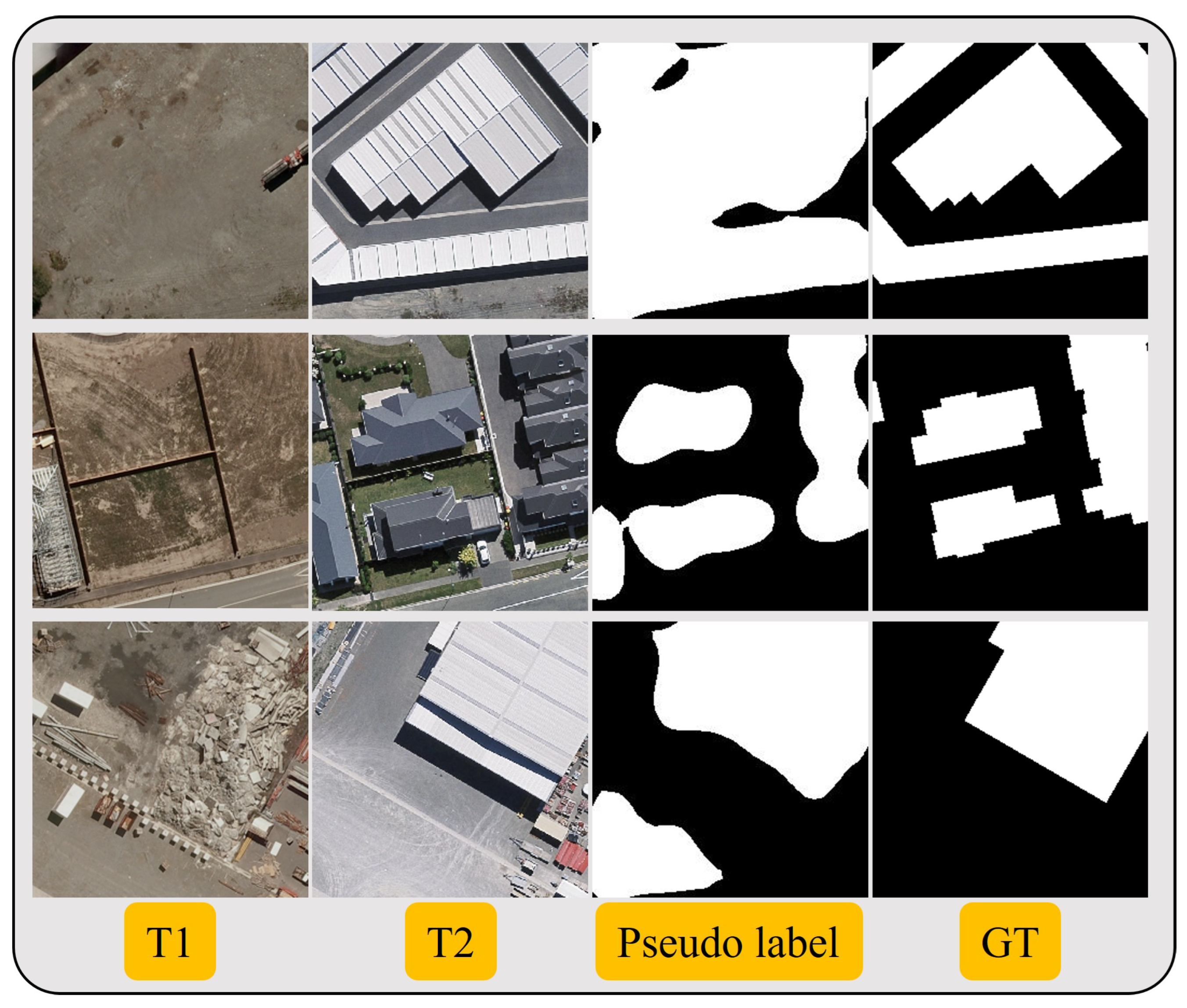
Although SSCD methods address the need for large amounts of labeled data, several challenges persist. On the one hand, when a small amount of labeled data is available, pseudo-changes have a large influence on the quality of pseudo-labels. Figure 1 shows some examples, which are from the WHU-CD [35]. In this case, the quality of pseudo-labels needs to be improved. On the other hand, for SSCD networks and training strategies, firstly, many current methods rely on ResNet50 [31] or Unet++ [30] for feature extraction, but these networks do not fully leverage features at different scales when generating change features, resulting in the inadequate recognition of multi-scale change buildings. Secondly, the learning bias inherent in semi-supervised methods, such as self-supervision and consistent regularization, combined with the simplistic approach to generating change features, often struggles to overcome pseudo-changes, leading to recognized change targets lacking detail. Thirdly, current SSCD methods based on consistency regularization typically only utilize multi-view predictions of input or encoder outputs for supervised training on unlabeled data. However, a single supervised signal does not effectively update the shallow parameters of the stacked network and limits the exploration of the perturbation space within the consistency framework. To alleviate these problems, we introduce a novel SSCD network named MSFGNet-SemiCD. This network adopts a Siamese structure and leverages multi-scale difference feature interaction, combining deep and shallow features to enhance feature representation. Additionally, it incorporates input perturbation and feature perturbation to generate multiple supervised signals, reducing the impact of pseudo-changes and learning biases on model performance. We conduct relevant experiments on publicly available change detection datasets, and the experimental results demonstrate the effectiveness of our proposed network. The main contributions of this paper are summarized as follows:

• This paper presents a novel semi-supervised change detection approach, denoted as MSFG-SemiCD. The method improves the feature representation using a designed feature extraction network and deeply supervises the model’s training jointly with input and feature perturbation to obtain more reliable pseudo-labels.
• A novel multi-scale difference feature fusion-guided change detection network (MSFGNet) is introduced in this study. The network is designed to incrementally extract bitemporal difference information, fuse features, and incorporate complementary details from various scales through a temporal difference guidance module, a full-scale fusion module, and a deep semantic guidance module.
• Extensive experiments and detailed ablation studies were conducted on four data scales (1%, 5%, 10%, and 20%) using two binary change detection datasets, WHU-CD and LEVIR-CD. The results clearly show the effectiveness of our method in leveraging unlabeled data.

2. Related Works

2.1. Consistency Regularization Methods

The method of consistency regulation has received great attention in many areas. It is mainly based on two basic assumptions, namely the low-density separation assumption and the clustering assumption, and assumes that it will obtain consistent results when the model represents different perspectives for the same input, i.e., the model is not affected by these disturbances. According to the monitored signal, unlabeled data updating methods can be categorized into feature updating [36] and model updating [37]. Unlike the above methods, some other methods make consistent predictions based on different perspectives of the data, where choosing the right perturbation method and adding the perturbation at the right place is crucial for learning the distribution of unlabeled data. In [26,38,39,40,41], several shape and color perturbation methods for the image at the input are developed and combined with certain rules to create multiview input data. In [27], the authors add noise to the features in the model by observing and reflecting on domain-specific tasks and constructing relevant methods to meet the requirements of a specific task. Chen et al. [42] set different initial values for the two semantic segmentation networks to achieve coherent network-level prediction. Yang et al. [34] argued that the perturbations in the FixMatch method were too homogeneous and relied too heavily on manually designed perturbations. For this reason, a combination of multi-perspective perturbations is developed to apply perturbations in multiple locations, promoting the exploration of spatial diversity of perturbations through consistency methods.

2.2. Semi-Supervised Change Detection

Unlike fully supervised CD, SSCD typically obtains a priori knowledge from a small number of labeled bitemporal images before mining information from a large number of unlabeled bitemporal images. Recently, some CD scholars have attempted to use large numbers of unlabeled image pairs. Peng et al. [30] constructed a segmentation network instead of a generator and then performed segmentation and entropy map prediction to exploit the consistency of the distributions of the labeled data and the unlabeled data. On the other hand, scholars have conducted extensive research based on consistency regularization; ref. [32] think about consistency regularization from the CD perspective and believe that the semantic feature depth change representations in change detection better satisfy the consistency regularization assumption, so change features are randomly perturbed in several predefined feature perturbations. Ref. [31] designed an incremental SSCD using the Feature Prediction Alignment (FPA) method, which combines data perturbation consistency and cross-spatial category alignment to reduce prediction uncertainty. The authors of [33] performed combined color and shape perturbation at the input data. The authors of [43] first performed rotation and non-rotation operations on unlabeled data, after which the two data obtained were severely disturbed. The unrotated samples are then directly monitored using pseudo-labels, and the rotated samples are weighted using uncertainty categories to achieve consistent predictions. Unlike the perturbation approach at the input and the features, ref. [44] constructed a task-level consistency regularization method that unifies semantic segmentation and change detection tasks under the same framework through the use of building labels at a single timeDistinguishing consistency regularization methods that directly utilize multi-view data for supervised training, some scholars have attempted to utilize a self-training framework for the quality control of pseudo-labels generated from unlabeled data. In [28], by combining self-training and consistency methods, a self-supervised approach is used to filter the unlabeled data to obtain reliable unlabeled data, and finally, the model is retrained using a consistent regularization strategy and the newly created dataset. The authors of [29] use a self-trained model to build an SSCD. To ensure the method’s performance, two main considerations are made, including using contrast learning to improve the feature extraction ability of the model for the target and exploiting the uncertainty of the unlabeled data to select reliable pseudo-labels. All of the above methods use a combination of multiple learning strategies or multiple supervised signals to achieve excellent performance.

3. Methodology

3.1. MSFG-SemiCD Framework

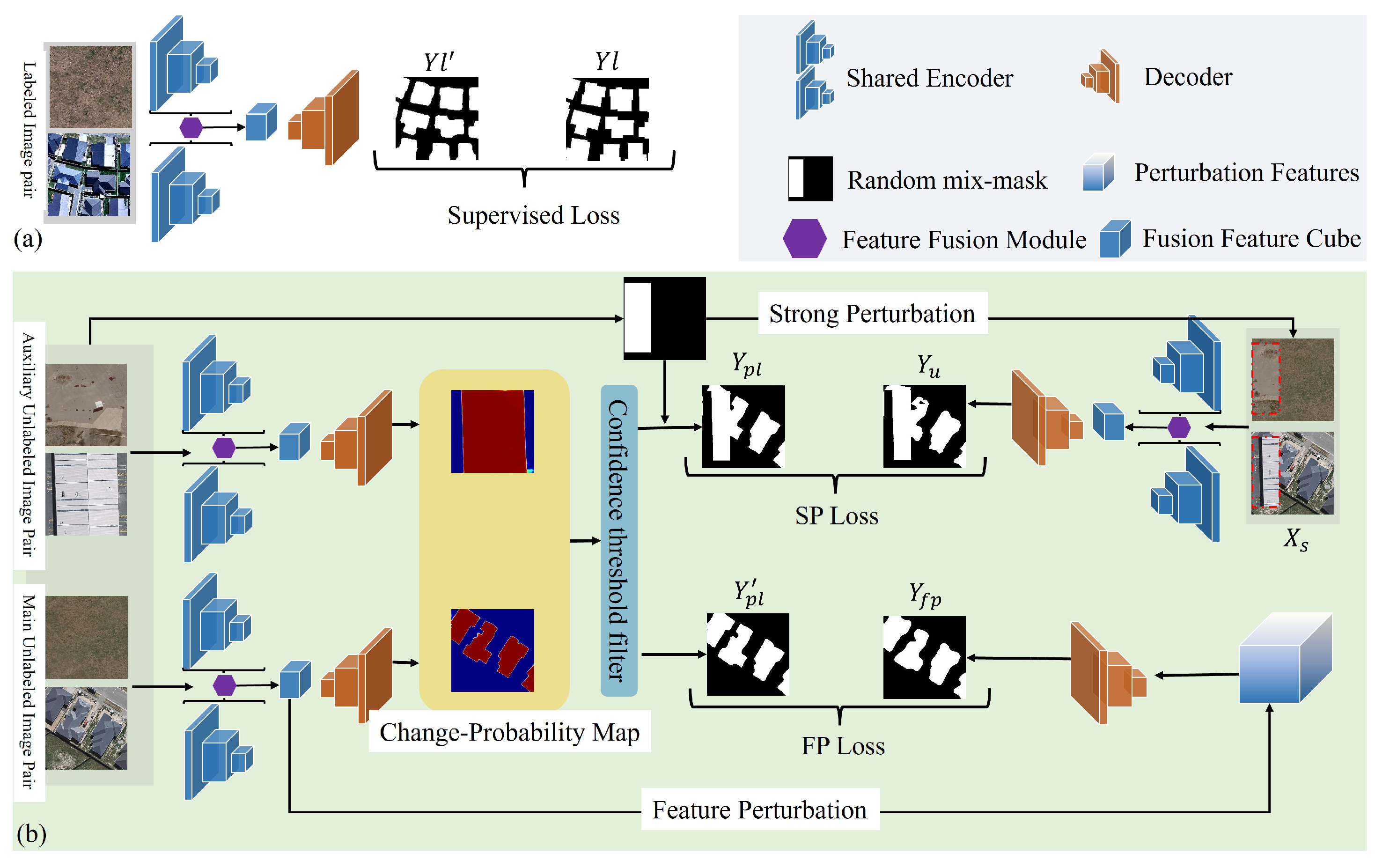
The flow of the proposed method, as shown in Figure 2, primarily includes supervised and unsupervised components. Labeled bitemporal image pairs are input into the network in the supervised phase (shown in Figure 2a). The loss is then calculated based on the prediction results $Y{l}^{\prime }$ with binary labels $Yl$. On the other hand, the unsupervised phase (shown in Figure 2b) includes two main operations: input perturbation and feature perturbation. For input perturbation, both main and auxiliary unlabeled image pairs are simultaneously provided to the model to generate pseudo-labels $Y_{pl}$, $Y_{pl}^{\prime }$ and prediction results $Y_u$. First, weak perturbation is applied to all unlabeled data, followed by two processing streams. In the first stream, data are fed into the model to produce probability maps, which are then filtered using mixing masks and confidence thresholds to obtain high-confidence pseudo-labels $Y_{pl}$ and low-uncertainty pseudo-labels $Y_{pl}^{\prime }$ for main unlabeled data. In the second stream, weakly perturbed data creates mixed image pairs $X_s$ by mixing masks and strong perturbations, which are subsequently fed into the model for predictions $Y_u$. Feature perturbation performs random feature perturbation on the feature cube generated by the encoder for primary unlabeled image pairs. These perturbed features are fed into the decoder to obtain the perturbation prediction $Y_{fp}$. Finally, the unsupervised loss is calculated based on the pseudo-labeled $Y_{pl}$, $Y_{pl}^{\prime }$ and predicted $Y_u$, $Y_{fp}$. A weighted summation of the supervised and unsupervised losses determines the total loss $L_{cd}$. The network parameters are then updated by backpropagation of $L_{cd}$.

3.2. Input Data Perturbation in MSFG-SemiCD

The perturbation techniques in this study can be divided into input perturbation and feature perturbation. The input perturbation is further divided into weak and strong perturbation (see Figure 3). Weak perturbation is common data augmentation, such as random flip and random cropping, which are often used to expand the dataset and improve the robustness of the model. On the other hand, strong perturbations disturb the input data to a greater extent in terms of color or shape, thus distorting the data. For the better construction of multiview inputs, we further implement strong perturbations after data augmentation of the input unlabeled data with the help of RandAugment (we randomly select 2 out of 10 predetermined color transformations) [40] and Cutmix [45]. Feature perturbation applies operations to the encoder’s intermediate or output features to prevent the model from relying too heavily on certain features, thereby increasing its resilience to perturbation. In contrast to the tailored feature perturbation methods in RCR [32], existing perturbation techniques in the PyTorch framework (e.g., Dropout2D) are directly applied to mask a part of the feature layer in the encoder’s output feature cube, which the creation allows multiview feature inputs and the acquisition of additional supervised signals.

When performing hybrid perturbation, it is critical to maintain the consistency of the bitemporal image. Unlike the Cutmix operation on a single image, bitemporal image perturbation requires using a pair of auxiliary image pairs to mix data and preserve temporal information. When introducing shape perturbation, applying the same shape transformation to pseudo-labels is important to align prediction results and pseudo-labels in pixel space during consistency prediction for multi-view input data.

3.3. Multiscale Feature Fusion and Semantic Guidance Network (MSFGNet)

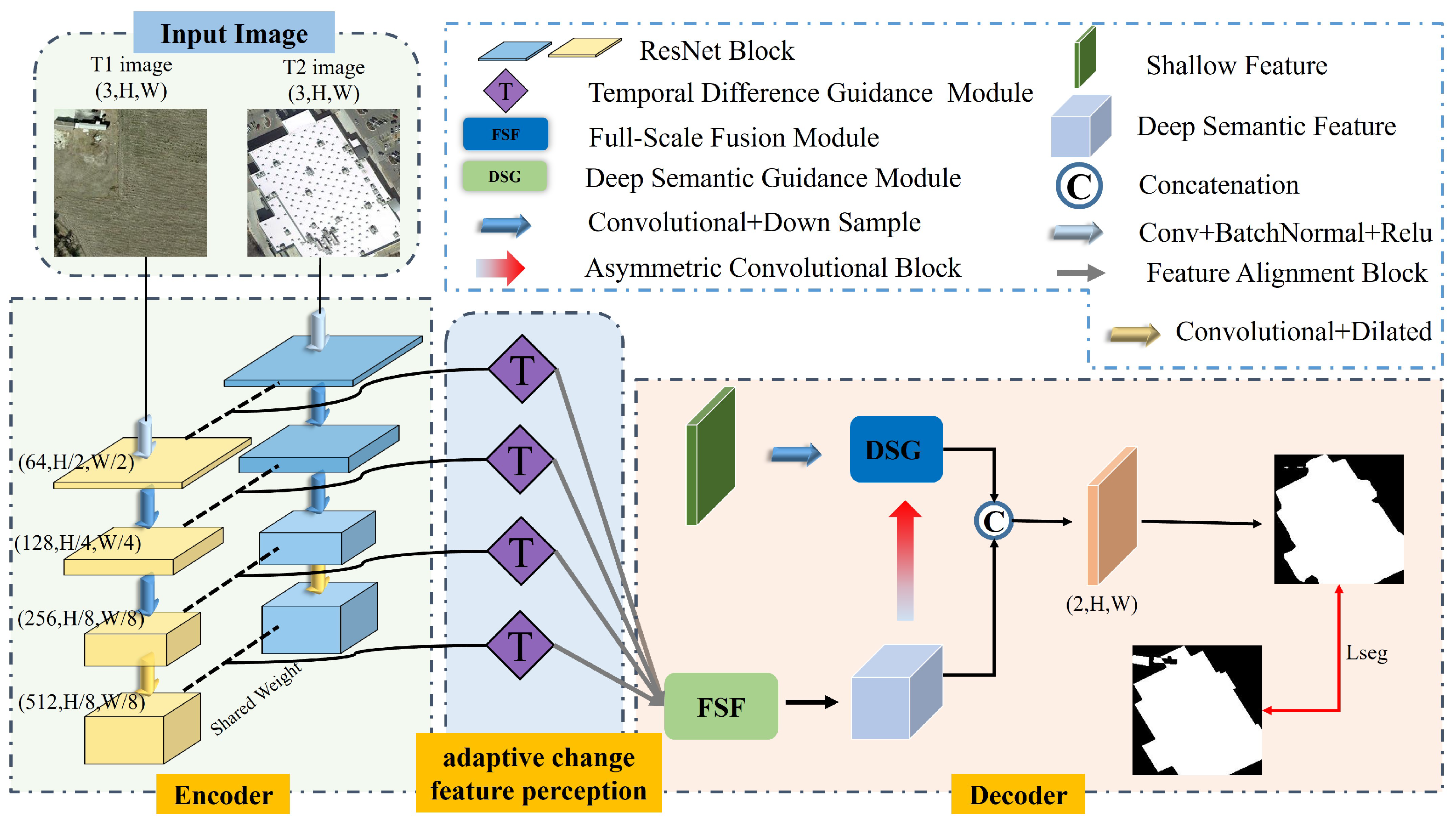
The network structure shown in Figure 4 comprises three main components: an encoder, an adaptive change feature perception module, and a decoder. Initially, a pair of aligned bitemporal images, T1 and T2, are input into a weight-sharing Siamese network, which includes ResNet-18 [46] for separate encoding. This process hierarchically transforms the bitemporal images from RGB color space to various high-level feature spaces. To preserve the spatial resolution of deep semantic features and gather more contextual information, dilated convolution is applied to the final layer of down-sampled features, resulting in a set of features with a larger receptive field and diverse representations but consistent spatial resolution. The extracted features can be expressed as $F_{t1}^i$ and $F_{t2}^i$, where $i\in \left\{1,2,3,4\right\}$, and the corresponding channel numbers are 64, 128, 256, and 512. The adaptive change feature perception incorporates four temporal difference guidance (TDG) modules to integrate and enhance coarse change features, extracting precise information on the differences between the bitemporal features. Different features at different scales are aligned using an adapter in the feature fusion guide module. Subsequently, a dilated convolution group refines the unified feature to create a semantically rich feature cube for multiscale variation target capture and refinement. Then, shallow change features are introduced to compensate for semantic features’ lack of detailed expression. To eliminate the effects of cross-scale feature fusion, deep semantic features guide learning shallow features to promote fusion and complementary information between the two. Finally, the fused features are passed through a simple decoder to generate the change map.

3.3.1. Adaptive Change Feature Perception

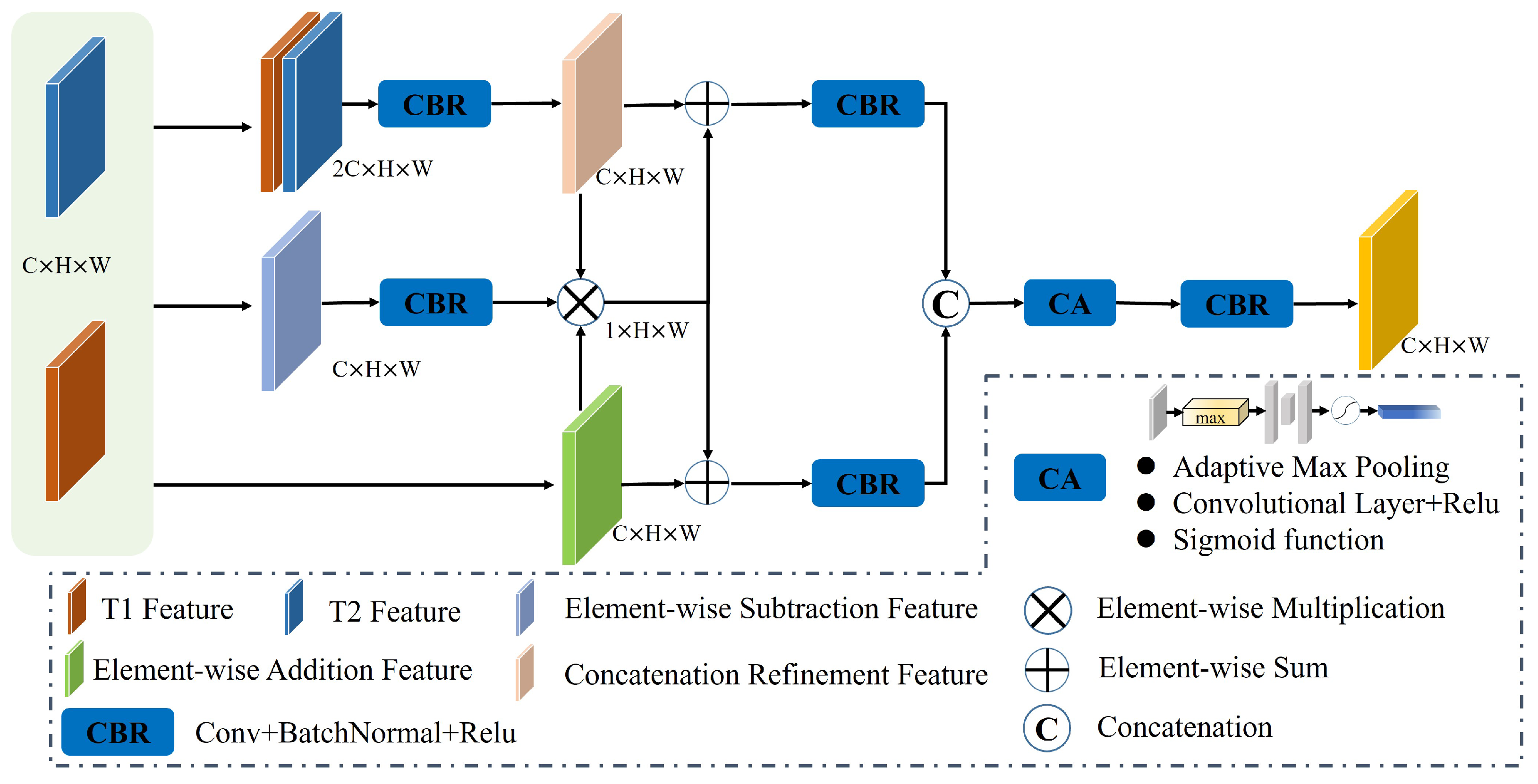
After encoding, the original image is transformed into multilevel features. Effective feature aggregation is crucial for improving change detection performance. Previous methods have utilized feature channel concatenation, element subtraction, and element addition. However, these methods have limitations in effectively aggregating bitemporal features to capture semantic differences, which is detrimental to change detection tasks. To address this issue, we propose that the TDG integrate diverse initial difference information and enhance the expression of semantic differences in bitemporal features. In Figure 5, we illustrate this process using the bitemporal feature of layer i as an example. Initially, we obtain three coarse difference features ($F_c$, $F_s$, and $F_a$) through channel concatenation, element subtraction, and element addition.

Considering that the subtraction can intuitively obtain the differences between features, we refine the difference feature $F_s$ and use the Sigmoid function to convert the refined $F_s$ into weight map $Att$, which is used to guide the other two features for learning the bitemporal change. Which can be obtained as follows:

$$\begin{array}{c}Att=Sigmoid\left({Conv}_{3\times 3}\left({Conv}_{3\times 3}\left(F_s\right)\right)\right)\end{array}$$

(1)

Since the concatenation is only a merge of the bitemporal feature channel, the direct use of this part of the feature can only be learned by the backpropagation algorithm to learn the embodiment of different features. For the RSCD task, the features after channel concatenation do not highlight the temporal difference information. For this reason, we utilize a convolution operation to learn the correlation between the concatenation of bitemporal features. Subsequently, the features are fine-tuned and aligned using $1\times 1$ convolution. The formula is represented as follows:

$$\begin{array}{c}{F}_c^{\prime }={{Conv}_{1\times 1}(Conv}_{3\times 3}\left(F_c\right))\end{array}$$

(2)

$F_c^{\prime }$ represents the change features that are fine-tuned by channel concatenation. After that, $F_c^{\prime }$ and $F_a$ are multiplied with the weight $Att$ to highlight the change region to obtain the enhanced representation of the change features in different perspectives, respectively. Then, we combine the enhanced features with the original features to improve the representation of features. The details are as follows:

$$\begin{array}{cc}\hfill F_c^{\prime \prime }& ={Conv}_{3\times 3,c}(F_c^{\prime }\times att+F_c^{\prime })\hfill \\ \hfill F_a^{\prime }& ={Conv}_{3\times 3,c}(F_a\times att+F_a)\hfill \end{array}$$

(3)

where $F_c^{\prime \prime }$ and $F_a^{\prime }$ denote the change features of concatenation and addition reinforced by weights $Att$, respectively. In order to learn the change semantic information from multiple perspectives, we introduce the channel attention mechanism (CA) to deal with the two difference features $F_c^{\prime \prime }$, $F_a^{\prime }$, according to the perception of the change target to adaptively obtain the importance of the difference features, to realize the weight allocation of the difference features, and ultimately to enhance the network’s ability to perceive the change features. The formula is as follows:

$$\begin{array}{c}{F}_i={Conv}_{1\times 1,c}\left(CA(F_c^{″},F_a^{\prime })\right)\end{array}$$

(4)

3.3.2. Feature Fusion Guidance Module

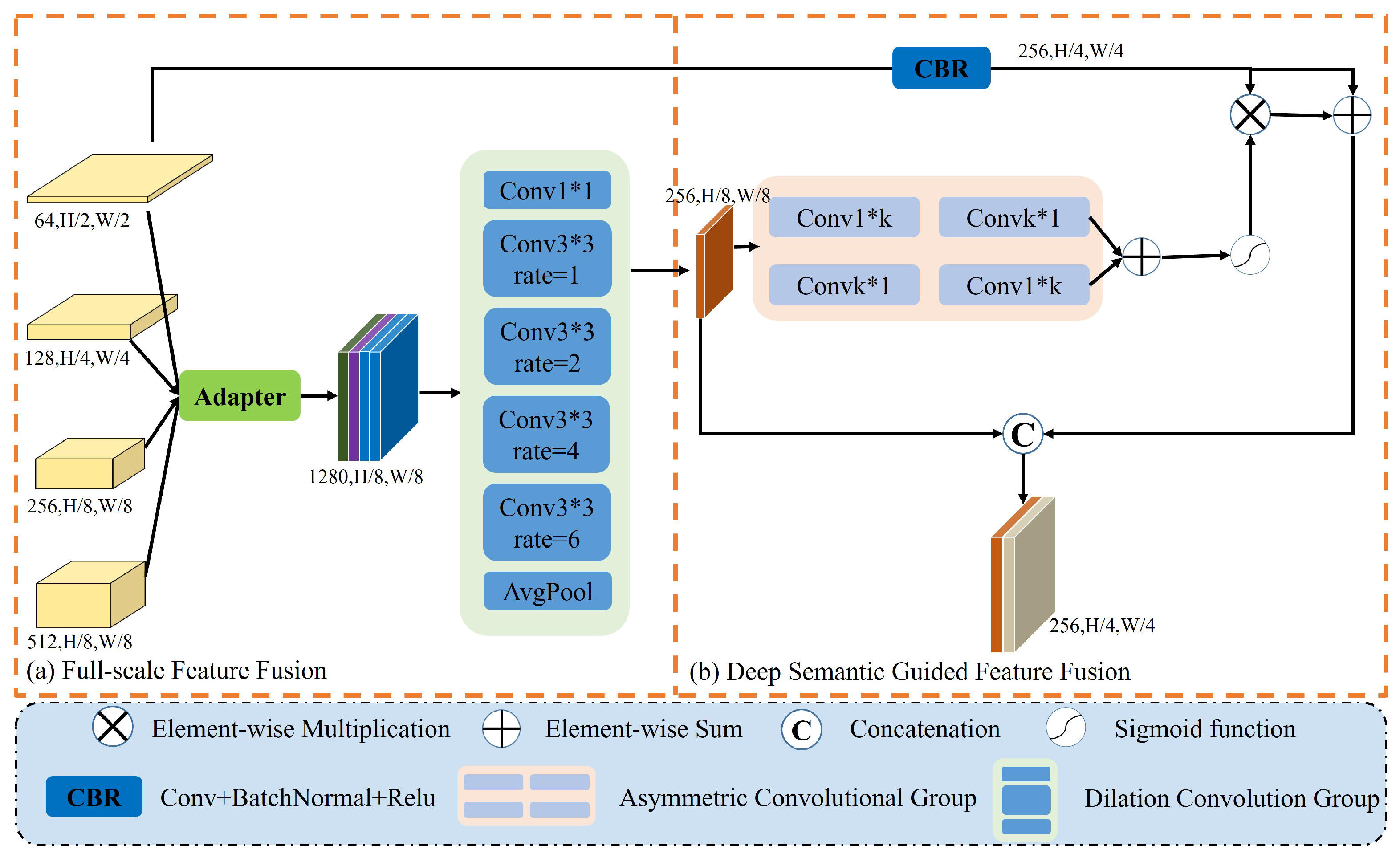
Unlike previous SSCD methods, where only the last layer of semantic features is used to obtain change features by element subtraction, we utilize the TDG module to obtain a multilevel representation of change features. For RSCD, the rich semantic information of deep features can localize the change target well, while the detailed information in shallow features aids in detecting the exact location of the change. Therefore, there is a need to address the fusion of multilevel change information. However, due to the differences between shallow and deep features, the direct fusion of change features at different scales may lead to interference information, resulting in the degradation of feature expression. As shown in Figure 6, to ensure that different features can complement each other in information extraction and improve the expression ability when aggregated, the full-scale difference features are first aligned using an adapter. Subsequently, the uniformly represented features are filtered for background noise, fine-tuned for their semantic position using the dilated convolutional group, and mined for change information at multiple scales. In addition, to obtain more complete change detection results and alleviate the problem of learning bias in semi-supervision, we introduce shallow features to supplement the detailed information. However, a direct cross-scale fusion of deep semantic information with shallow features brings about performance loss; for this reason, we design a deep semantic guidance module to guide the learning of shallow features and facilitate the fusion of deep and shallow features.

Full-scale feature fusion: Multilevel difference features provide information about changes between bitemporal data at various scales. To better leverage the benefits of features at different scales and enhance the interaction of multiscale information, adapters are used to unify the representations of features at different levels and facilitate the fusion of features across scales. Initially, convolution operations are applied to different features for refinement and alignment. To prevent issues like gradient explosion or vanishing gradients and ensure the training process’s stability, batch normalization and nonlinear activation operations are incorporated. The details are described below:

$$\begin{array}{c}{cf}_j=RELU\left(BN\left(Conv\left(k,s,p\right)\left(F_i\right)\right)\right)\end{array}$$

(5)

where i denotes the feature layer $i\in \left\{1,2,3,4\right\}$. k, s, and p represent the convolution kernel size, step size, and padding rate, respectively. BN denotes the batch normalization, and RELU is the nonlinear activation function. When $i\in \left\{1,2\right\}$, we uniformly set k = 3, s = 2, p = 1, mainly used to increase the diversity of feature expression and adjust the feature size. When $i\in \left\{3,4\right\}$, k = 3, s = p = 1, which is mainly used here to increase the diversity of feature expression. Then, we can obtain the feature map ${cf}_j\in R^{c_i\times h\times w}$, $j\in \left\{1,2,3,4\right\}$. The ${cf}_j$ denotes the unified representation of features under different levels.

As shown in Figure 6a, the features after unified representation are concatenated on the channel. Then, we utilize the dilated convolution group to fine-tune the features to obtain a finer semantic representation. The formula is expressed as follows.

$$\begin{array}{cc}\hfill R_i& =RELU\left(BN\left({Conv\left(k,d,p\right)}_i\left(cat\left({cf}_j\right)\right)\right)\right)\hfill \\ \hfill R& =RELU\left(BN\left({Conv}_{3\times 3}\left(cat\left(R_i\right)\right)\right)\right)\hfill \end{array}$$

(6)

where k, d, and p represent the convolution kernel size, dilation rate, and padding rate, respectively. When $i=0$, we uniformly set k = 1, d = 0, p = 0, which promotes the flow of information between channels. When $i\in \left\{1,2,3,4\right\}$, we set k = 3, d = $\left\{1,2,4,6\right\}$, p = $\left\{1,2,4,6\right\}$, respectively. When $i=5$, we use global average pooling to obtain the global semantic representation. With the above steps, we can obtain the feature maps $R_i\in R^{c/r\times h\times w}$, $i\in \left\{0,1,2,3,4,5\right\}$ for different receptive fields, where r is mainly used to reduce the number of channels, and we set r to 4 in our experiments. R is a further refined and integrated representation of the feature $R_i$.

Deep semantic guidance: To improve the completeness of change features and mitigate learning bias in semi-supervised learning. We introduce shallow features to complement the details in the deep features. However, considering the semantic gap between deep and shallow features, we utilize the localization ability of deep features to construct a learning weight to guide the learning of shallow features that promotes the fusion of deep and shallow features. As shown in Figure 6b, for the strengthened feature R, we utilize a pair of vertical kernels and horizontal kernels of the convolution group instead of the large kernel $(K\times K)$ to reduce the computational load while further expanding the receptive field and obtaining more global attention. After that, we perform element addition and Sigmoid operations on two feature maps, $X_1$ and $X_2$, to obtain the feature spatial location importance weight map $X_{att}$. The formula is depicted as follows:

$$\begin{array}{cc}\hfill X_1& ={Conv}_{11\times 1,1}\left({Conv}_{1\times 11,c}\left(R\right)\right)\hfill \\ \hfill X_2& ={Conv}_{1\times 11,1}\left({Conv}_{11\times 1,c}\left(R\right)\right)\hfill \\ \hfill X_{att}& =Sigmoid(X_1+X_2)\hfill \end{array}$$

(7)

Shallow features contain a mix of high-frequency information and noise, making it challenging to extract useful knowledge. In order to improve the effectiveness of learning from these shallow features, we fine-tune them. We then use a weight map to highlight the change regions and enhance the shallow features. By summing the shallow raw features with the enhanced ones, we aim to improve the overall feature representation. The detailed formulation is provided below:

$$\begin{array}{cc}\hfill F_l& =RELU\left(BN\left({Conv}_{3\times 3}\left(F_1\right)\right)\right)\hfill \\ \hfill F_l^{\prime }& ={Conv}_{3\times 3}(F_l\ast X_{att}+F_l)\hfill \end{array}$$

(8)

where $F_1$ denotes the first layer of change features, $F_l$ denotes the fine-tuned shallow features, and $F_l^{\prime }$ denotes the shallow enhanced features. Finally, the deep and shallow features are combined and fed into the decoder through the concatenation operation to promote the fusion between deep and shallow features, thus optimizing the final binary change map $M_b$.

$$\begin{array}{c}{M}_b=Decoder\left(Concat\left(up\left(R\right),F_l^{\prime }\right)\right)\end{array}$$

(9)

3.4. Loss Function Definition

3.4.1. Supervision

As shown in Figure 2a, only the labeled data are used to optimize the network parameters to give the network a preliminary change prediction capability in this phase. First, we create a pixel-level change prediction map $Y_i^{\prime }$ for the labeled data in the labeled dataset $D_l={\left\{\left\{X_{li},{X^{\prime }}_{li}\right\},Y_{li}\right\}}_{i=1}^N$ (where $\left\{X_{li},{X^{\prime }}_{li}\right\}$ denotes the i-th pair of bitemporal images, $Y_{li}$ denotes the corresponding ground truth, and N is the size of the labeled dataset). Then, a standard cross-entropy loss is used to estimate the difference between the prediction $Y_i^{\prime }$ and the ground truth $Y_{li}$, which is expressed as follows:

$$\begin{array}{c}{L}_{sup}=CE\left(Y_i^{\prime },Y_{li}\right)\end{array}$$

(10)

3.4.2. Unsupervised

As shown in Figure 2b, in this phase, we trained the model with unlabeled data $D_{ul}={\left\{\left\{X_{uli},{X^{\prime }}_{uli}\right\}\right\}}_{i=1}^M$ ($\left\{X_{uli},{X^{\prime }}_{uli}\right\}$ denotes the ith pair of unlabeled images, and M denotes the size of the unlabeled dataset, which is usually assumed to be larger than the number of labeled datasets N) and learn the perturbation-invariant feature representations to improve the performance of the model. To achieve this, we set an unsupervised loss function $L_{us}$ for unlabeled images, which consists of two parts: the input perturbation consistency loss $L_{sp}$ and the feature consistency loss $L_{fp}$. First, pixel-level probability distribution prediction maps $P_j^i$ are obtained for weakly perturbed unlabeled image pairs. To achieve supervised prediction results for highly noisy inputs, pseudo-labeled maps $Y_{uli}$ are generated in the following way:

$$\begin{array}{c}{Y}_{uli}=argmax\left(P_j^i\right)\end{array}$$

(11)

The obtained map $Y_{uli}$ represents the maximum probability value corresponding to each pixel in the feature map. However, in order to achieve the high-quality monitoring of various disruption predictions, it is necessary to exclude those predictions with high uncertainty; i.e., the pseudo-labels are filtered by noise, and the confidence map $Y_m^c$ is generated by filtering on a confidence threshold as follows:

$$\begin{array}{c}{Y}_m^c=\left\{\begin{array}{ccc}1,\hfill & \mathrm{if}\hfill & Y_{uli}>\tau \hfill \\ 0,\hfill & \mathrm{else}\hfill \end{array}\right.\end{array}$$

(12)

Here, for the element’s value at each position in $Y_m^c$, if the probability value corresponding to the pseudo-label is greater than the threshold $\tau$, we set $\tau$ to the empirical value of 0.95 and 0 otherwise.

Therefore, for the consistency loss at the input, the pseudo-label is obtained by predicting the weak perturbation by the model and then predicting the strong perturbation $Y_u$, and the standard cross entropy is used as the loss function to measure the invariance of predicting various perturbations. The details are as follows:

$$\begin{array}{c}{L}_{sp}=CE\left(Y_u,Aug\left(Y_{uli}\times Y_m^c\right)\right)\end{array}$$

(13)

Here, $Aug(.)$ denotes the same perturbation operation as the input to ensure the consistency between pseudo-label and strong perturbation prediction results.

In contrast to the perturbation operation at the input, the feature perturbation only regulates the difference feature $f_{ulw}^d$ of the unlabeled weakly perturbed image. The pseudo-label is generated in the same way as above. In order to satisfy the consistency condition for the depth difference feature, the difference feature generated from the weakly perturbed image is mainly perturbed to generate the multi-view difference feature expression and ensure the prediction consistency of the difference feature in the prediction result, which is implemented as follows:

$$\begin{array}{c}{L}_{fp}=CE\left(f_d\left(f_{ulw}^d\right),f_d\left({f_{ulw}^d}^{\prime }\right)\right)\end{array}$$

(14)

where ${f_{ulw}^d}^{\prime }$ denotes the perturbation feature and $f_d(.)$ denotes the decoder used to obtain the prediction result. The final loss consists of the above two parts of the loss as shown below:

$$\begin{array}{c}{L}_{cd}=L_{sup}+{\lambda }_1{L}_{sp}+{\lambda }_2{L}_{fp}\end{array}$$

(15)

where ${\lambda }_1$ and ${\lambda }_2$ denote the participation weights of each part of the loss in the unsupervised loss, respectively.

4. Experiment

4.1. Experimental Setup

4.1.1. Datasets

To validate the effectiveness of the proposed method, we select two public high-resolution remote sensing image change detection datasets, the WHU change detection dataset (after that referred to as the WHU-CD dataset), and the LEVIR-CD dataset.

WHU-CD [35]: The dataset contains five images, including two remote sensing images taken in Christchurch, New Zealand, in 2012 and 2016, and the building label maps and change maps associated with each image. Each image has the same dimensions, with a size of 32,207 × 15,354 and a pixel resolution of 0.2 m. Due to the intensive reconstruction work after the earthquake, the main changes revolved around buildings.

LEVIR-CD [21]: This is a much larger, high-resolution data set for detecting building changes. It was obtained from Google Earth and mainly contained 637 pairs of 1024 × 1024 images with a pixel resolution of 0.5 m acquired between 2002 and 2018 from 20 different areas in several cities in Texas, USA.

4.1.2. Data Preprocessing

Due to GPU memory limitation, we split the raw data into non-overlapping 256 × 256 pixel blocks. Among them, in the WHU-CD dataset, we divided the data using a split ratio of 8:1:1, and in the LEVIR-CD dataset, we divided the data following the original division given in the dataset, which are used for training, validation, and testing, respectively. To facilitate subsequent experiments, this paper collects random data with sampling rates of 1%, 5%, 10%, and 20% to generate semi-supervised training datasets for different scenarios (see

Table 1. Division of the semi-supervised training dataset.

Labeled Ration	Train Data
	WHU-CD		LEVIR-CD
	Labeled	Unlabeled	Labeled	Unlabeled
1%	60	5887	71	7049
5%	298	5649	356	6764
10%	595	5352	712	6408
20%	1189	4758	1424	5696
Val/test	743/744		1024/2048

). In addition, resizing, cropping, and flipping operations were performed on the data to enhance the model’s generalization ability. Moreover, the consistency regularization method used in this paper requires different perspectives of the inputs to unlabeled data. In addition to weakly perturbing the unlabeled data, we perform a higher level of data enhancement operations to meet this condition. It (see Figure 3) mainly includes RandAugment and Cutmix operations, which have a greater impact on the original data in terms of color and shape, resulting in greater distortion of the image.

4.1.3. Implementation Details

Our model was built based on the Pytorch framework and trained, validated, and tested on a hardware device equipped with an NVIDIA GeForce GTX3080 graphics processor with 10 G memory. During the training process, we optimize the model using SGD. where the batch size and weight decay are set to 2 and 1 × 10⁻⁴, respectively. The initial learning rate is set to 1 × 10⁻³ and updated dynamically based on the number of iterations using the initial learning rate multiplied by ${(1-iter/max\left(iter\right))}^{0.9}$. Our proposed method was trained on the LEVIR-CD and WHU-CD datasets for 80 epochs, and the network reached a convergent state.

4.1.4. Evaluation Metrics

To better evaluate the performance of the model, we introduce four widely used evaluation metrics for semantic segmentation, including precision (P), recall (R), F1 score, intersection over union (IOU), and the range of each metric from 1% until 100%. The detailed definitions of the above metrics are as follows:

$$\begin{array}{cc}\hfill \mathrm{P}& ={\displaystyle \frac{\mathrm{TP}}{\mathrm{TP}+\mathrm{FP}}}\hfill \\ \hfill \mathrm{R}& ={\displaystyle \frac{\mathrm{TP}}{\mathrm{TP}+\mathrm{FN}}}\hfill \\ \hfill \mathrm{IOU}& ={\displaystyle \frac{\mathrm{TP}}{\mathrm{TP}+\mathrm{FN}+\mathrm{FP}}}\hfill \\ \hfill \mathrm{F}1& ={\displaystyle \frac{(2\times \mathrm{P}\times \mathrm{R})}{\mathrm{P}+\mathrm{R}}}\hfill \end{array}$$

(16)

where TP and TN denote the number of correctly detected changed and unchanged pixels, respectively; in contrast, FP denotes the number of unchanged pixels that are recognized as changed pixels. FN denotes the number of changed pixels that are recognized as unchanged pixels. The above metrics can comprehensively evaluate the model’s performance from different perspectives.

4.2. Results and Discussion

4.2.1. Comparisons on the WHU-CD Dataset

Quantitative and qualitative comparisons were performed using SOTA methods to validate the superiority of the methods. Six main methods are included: RCR [32], RCL [29], FPA [31], UniMatch [34], S4GAN [47] and AdvEnt [48]. In addition, fully-sup and only-sup result presentations are also included, which provide an easy reference to illustrate the performance difference between these semi-supervised and fully-supervised methods. Here, “Fully Supervised” indicates that all labeled data are involved in the training, and “Sup Only” indicates that training is performed only on labeled data sampled at the label rate. In addition, RCR is an SSCD method based on consistency regularization, RCL is a hybrid method that combines pseudo-labeling and contrast learning, and FPA is an SSCD implemented by unifying pixel prediction alignment and image crossing. Region prediction refers to category alignment. UniMatch is a semi-supervised semantic segmentation method that combines dual image and feature perturbation in the same framework. S4GAN and AdvEnt also come from the semantic segmentation domain but are implemented based on generative adversarial methods.

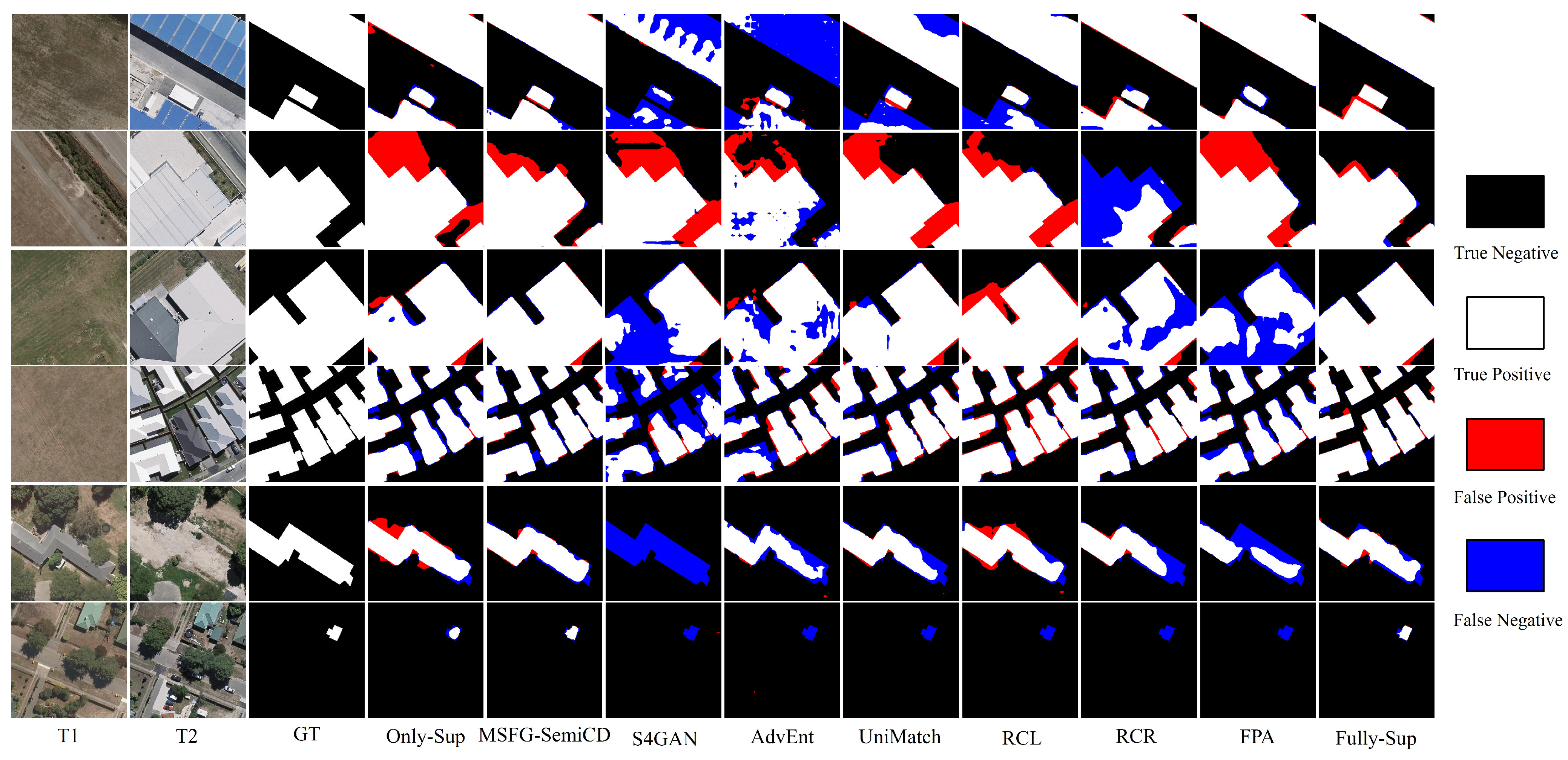
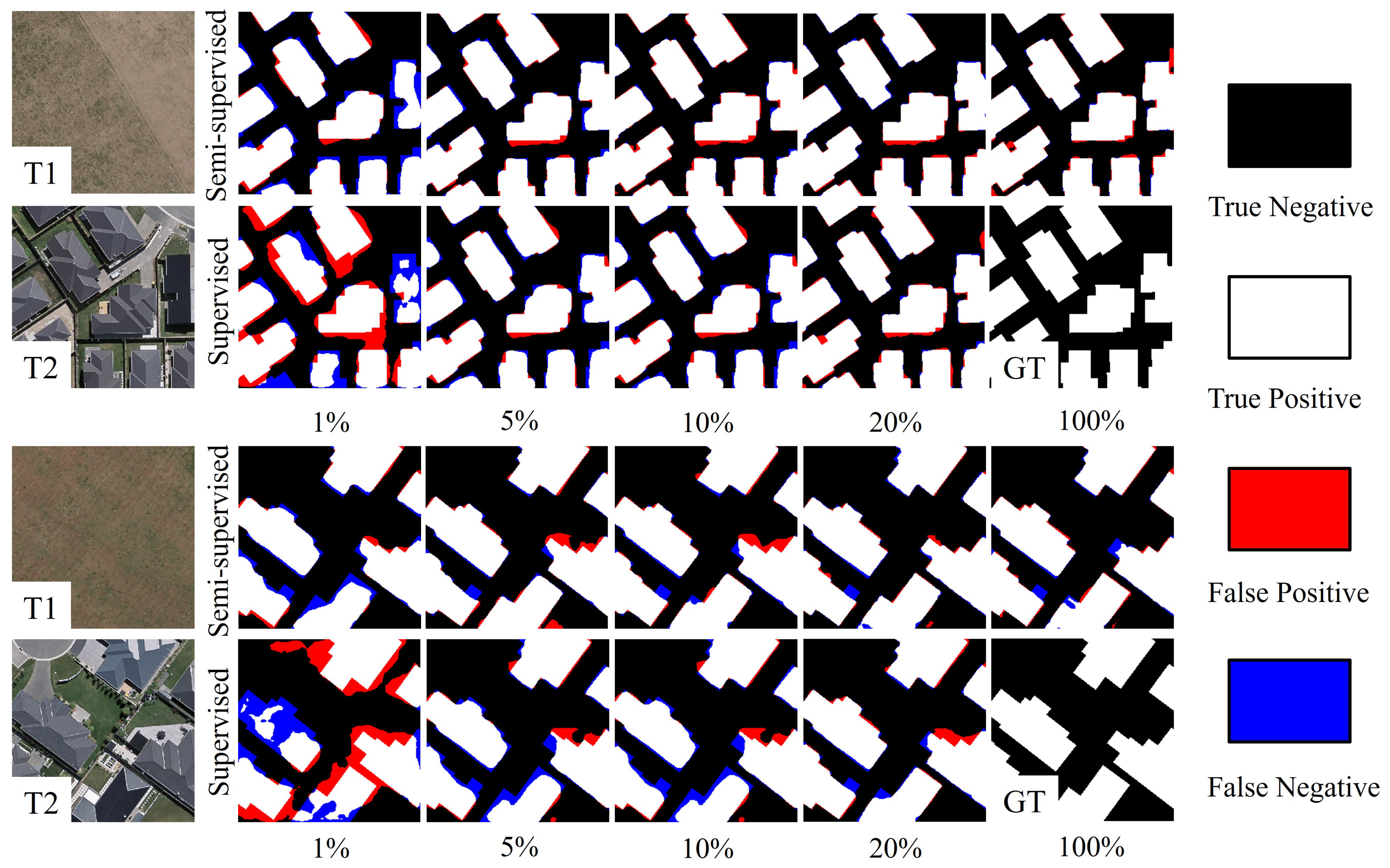
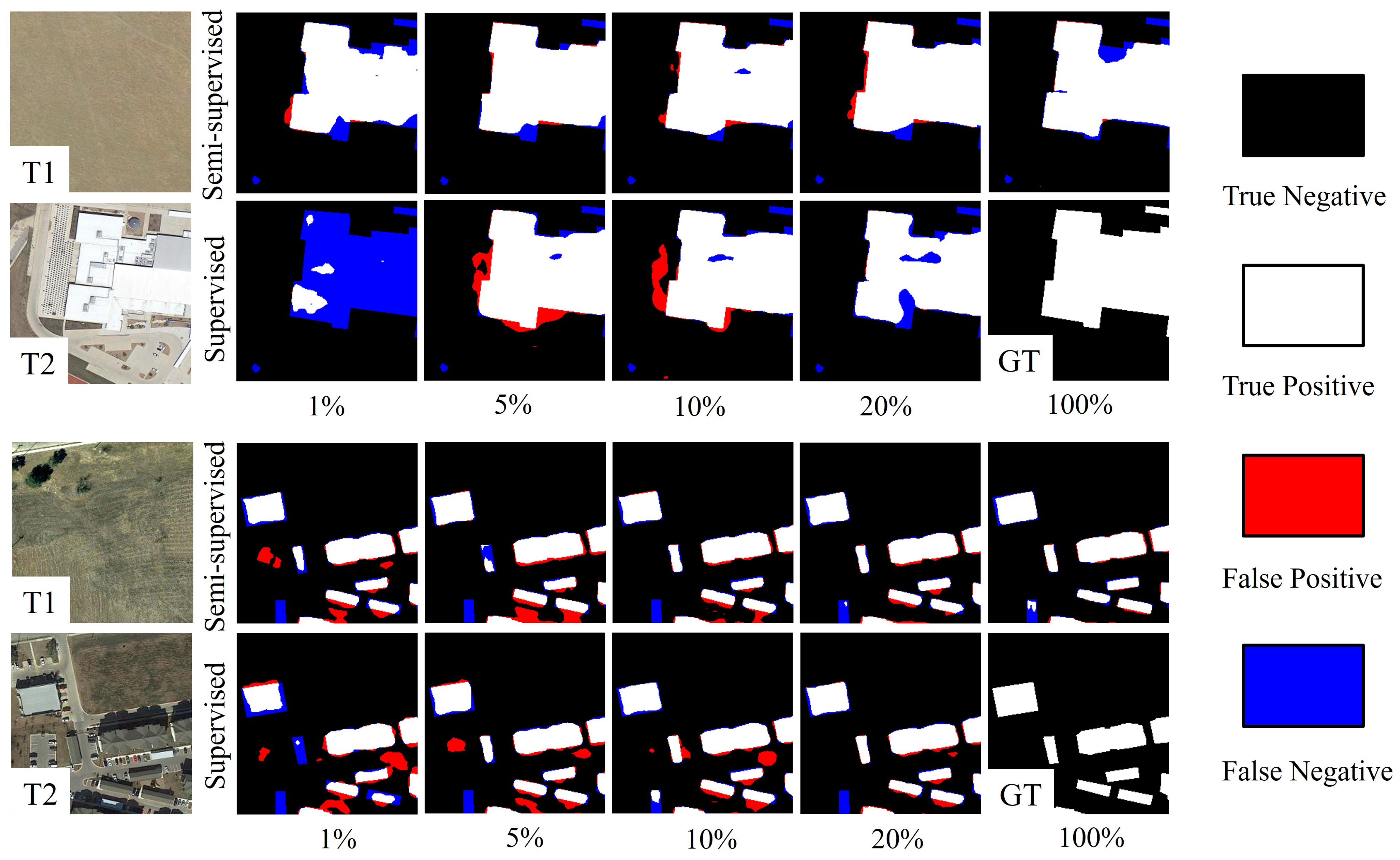
The outcomes of the WHU-CD dataset are displayed in Figure 7 and Figure 8. Among them, Figure 7 shows the visualization results of each model under 5%, and Figure 8 shows the visualization results of MSFGNet with different training styles under 1%, 5%, 10%, 20%, and 100% data. To make the visualization results more intuitive, we use black, white, blue, and red to denote TN, TP, FN, and FP, respectively. We can draw the following conclusions from the visualization results. First, with the increase in the available labeled data, there is a significant improvement in visualization for the edges, locations susceptible to false detections and omissions. Second, for large buildings with heterogeneous roofs and roof materials similar to other ground conditions, our method can overcome the effect of irrelevant variations well and obtain more complete identification results. Third, MSFG-SemiCD can recognize each change target completely in dense building areas and has a lower false detection rate than other methods. Fourth, our method can accurately localize the change target in some conditions with occlusion or complex background while obtaining relatively complete change results. This further indicates that MSFG-SemiCD can overcome pseudo-changes and obtain better detection results by weakening the effect of learning bias in semi-supervision through the complementary information of deep and shallow features.

The quantitative analysis is shown in

Table 2. Results of quantitative comparison experiments in the WHU-CD dataset.

Method	1%				5%
	IOU	F1	R	P	IOU	F1	R	P
Only-Sup	40.88	58.03	52.46	64.94	73.70	84.86	79.66	90.78
S4GAN	12.58	22.35	54.03	14.09	61.44	76.12	67.09	87.96
AdvEnt	19.39	32.48	19.50	97.21	65.44	79.11	68.64	93.36
UniMatch	44.03	61.14	48.68	87.69	75.32	85.92	79.67	93.24
RCL	45.26	62.31	48.03	88.69	73.89	84.98	85.50	84.47
RCR	53.89	70.04	66.49	73.99	77.47	87.31	84.73	90.04
FPA	43.47	60.60	46.64	86.50	78.91	88.83	87.94	89.74
MSFG-SemiCD	46.15	63.16	47.94	92.53	80.54	89.22	87.36	91.16
Method	10%				20%
	IOU	F1	R	P	IOU	F1	R	P
Only-Sup	78.20	87.77	86.60	88.96	79.25	88.42	84.74	92.43
S4GAN	70.38	82.61	80.57	84.76	69.05	81.69	81.22	82.17
AdvEnt	77.28	87.18	81.43	93.81	78.08	87.69	84.51	91.13
UniMatch	79.99	88.55	85.43	94.08	82.33	90.31	86.92	93.97
RCL	78.56	87.99	85.86	90.23	79.96	88.86	88.01	92.09
RCR	81.39	89.74	88.05	91.50	82.61	90.72	88.80	92.73
FPA	81.34	89.91	88.47	91.40	82.75	90.56	89.69	91.45
MSFG-SemiCD	83.49	91.00	91.79	90.23	84.80	91.78	90.31	93.29
Fully-Sup	(MSFGNet: 100%) → IOU = 87.29 F1 = 93.21 R = 92.47 P = 93.97

. When the proportion of labeled samples is 5%, 10%, and 20%, MSFG-SemiCD obtained the first performance. It outperforms the second FPA by 1.63%, 2.15%, and 2.05% on the IOU, respectively. In addition, the performance of MSFG-SemiCD improves by 5.27%, 6.84%, 5.29%, and 5.55% in IOU relative to Only-sup at 1%, 5%, 10%, and 20%, respectively, which further validates the ability of our approach to utilize unlabeled data to improve model performance. With 5% labeled data available, MSFG-SemiCD obtains the best performance improvement relative to other semi-supervised and supervised methods, which further demonstrates that MSFG-SemiCD can refine the performance of the model by learning a small amount of prior knowledge and then mining useful knowledge from a large amount of unlabeled data. However, in the extreme case of 1%, MSFG-SemiCD obtained the second-best results, with a difference of 7.74% from the first RCR. We analyze the two main reasons: the WHU-CD dataset has rich data types. Although in the extreme case of 1%, the model combined with the strong feature extraction capability of the PSPNet network is also well trained. Second, different training strategies in semi-supervision have different learning difficulties. Strong perturbations that transform colors and shapes cause damage to the data and are more difficult to learn relative to feature perturbations. Overall, our proposed method obtains good results on the WHU-CD dataset.

4.2.2. Comparisons on the LEVIR-CD Dataset

Table 3. Results of quantitative comparison experiments in the LEVIR-CD dataset.

Method	1%				5%
	IOU	F1	R	P	IOU	F1	R	P
Only-Sup	59.53	74.64	71.58	77.96	73.95	85.02	80.70	89.84
S4GAN	20.28	33.71	81.84	21.23	46.86	63.81	56.23	73.77
AdvEnt	49.95	66.62	51.53	94.20	59.68	74.75	62.02	94.05
UniMatch	75.83	86.26	85.59	86.94	74.56	85.43	81.46	89.80
RCL	67.69	80.73	77.64	84.07	71.75	83.55	82.33	84.80
RCR	65.37	79.06	73.29	85.81	75.24	85.87	82.06	90.05
FPA	69.62	82.09	78.61	85.89	77.00	87.00	85.03	89.07
MSFG-SemiCD	77.97	87.62	86.89	88.37	79.47	88.56	87.18	89.98
Method	10%				20%
	IOU	F1	R	P	IOU	F1	R	P
Only-Sup	77.71	87.46	86.18	88.77	78.21	87.77	85.03	90.69
S4GAN	52.34	69.71	76.88	62.11	55.09	71.04	70.85	71.24
AdvEnt	65.77	79.34	69.18	93.03	64.20	78.20	67.83	92.31
UniMatch	78.24	88.42	87.44	89.42	79.40	88.52	86.33	90.81
RCL	71.81	83.59	78.94	88.82	75.06	85.75	85.05	86.47
RCR	77.13	87.09	83.46	91.05	79.10	88.43	86.19	90.79
FPA	77.70	87.45	85.23	89.79	78.33	87.85	85.17	90.69
MSFG-SemiCD	79.90	88.83	88.01	89.66	80.39	89.13	87.72	90.59
Fully-Sup	(MSFGNet: 100%) → IOU = 83.81 F1 = 91.19 R = 90.11 P = 92.30

shows the quantitative evaluation results for the LEVIR-CD dataset. The LEVIR-CD is relatively large, but the data in the dataset are uniform across time scales and are not as rich as WHU-CD in terms of data richness, so the overall improvement in detection accuracy is lower than that of the WHU-CD dataset for 1%, 5%, 10%, and 20% increases in the amount of data. However, surprising results are obtained in the extreme case of 1%. MSFG-SemiCD obtains the best results with 1%, 5%, 10%, and 20% labeled data, outperforming the second FPA or UniMatch by 2.14%, 2.47%, 1.66%, and 0.99% in IOU. In addition, the performance gap between our model and other methods is maximized at the 1% and 5% data ratios, which further demonstrates the ability of MSFG-SemiCD to exploit large amounts of unlabeled data guided by a small amount of a priori knowledge. In addition, relative to partially semi-supervised methods, MSFGNet achieves performance outperformance with supervised training on a small amount of labeled data. The learning ability of semi-supervised methods in the LEVIR-CD dataset does not perform well. However, MSFG-SemiCD shows promising learning ability relative to other semi-supervised methods, with 18.44%, 5.52%, 2.19%, and 2.18% improvement in IOU relative to supervised methods at 1%, 5%, 10%, and 20% labeling ratios, respectively. This demonstrates our method’s ability to learn better in the LEVIR-CD dataset.

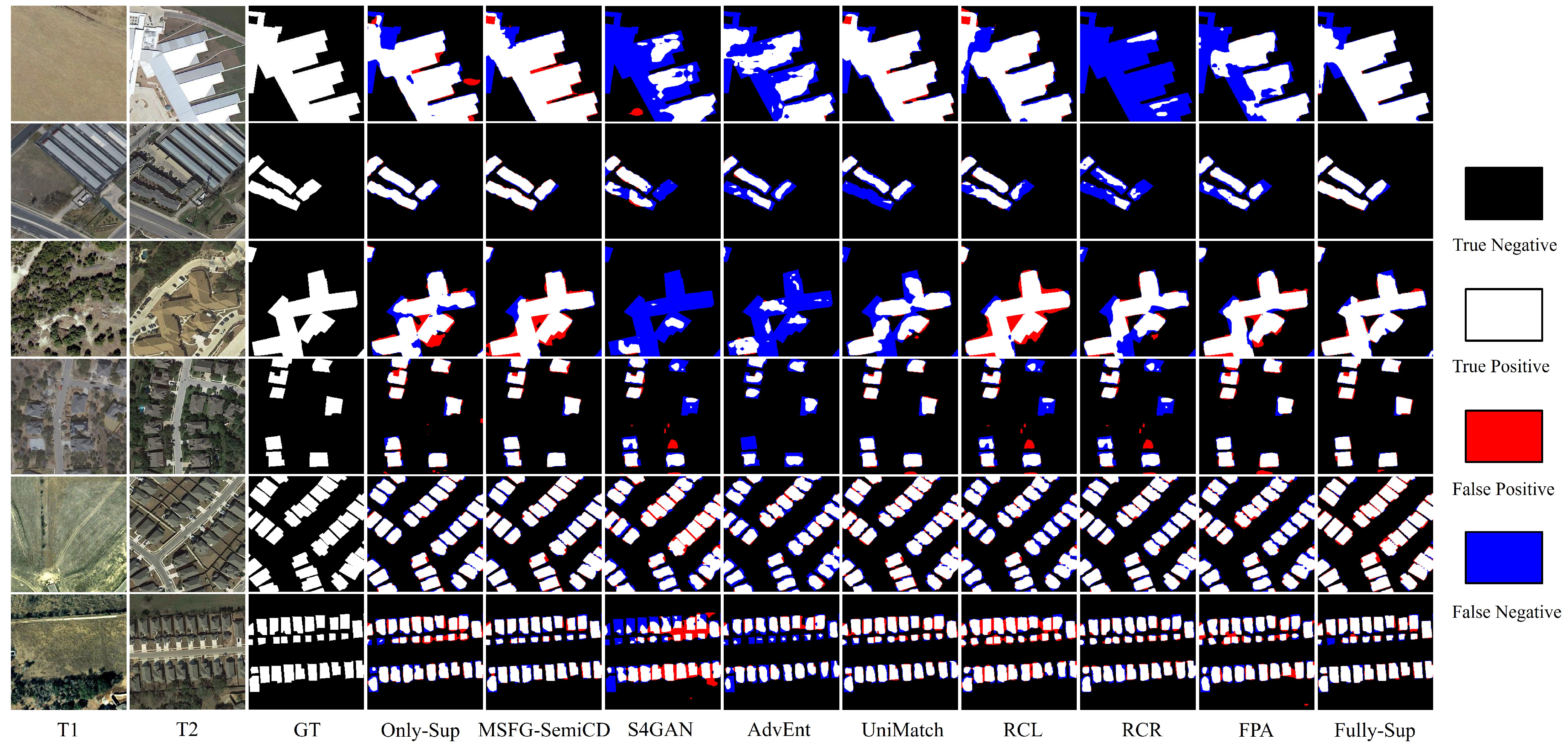
Figure 9 and Figure 10 show the visualization results in LEVIR-CD from different perspectives. Specifically, Figure 9 and Figure 10 show the detection results of different methods with 5% labeled data available and the detection results of MSFGNet under semi-supervised, Only-sup, and Fully-sup conditions, respectively. In Figure 9, the main focus is on changing buildings of different sizes, densities, and complex environments. For complex materials on the roofs of large buildings, MSFG-SemiCD can identify change areas as completely as possible. In dense and complex conditions, MSFG-SemiCD can accurately localize and identify the change regions while reducing the uncertainty of identification results at boundary locations and minimizing the interference of similar features. Figure 10 better shows the recognition results of MSFGNet under different training conditions. It can be seen that with the increase in the available labeled data, MSFG-SemiCD has better recognition results relative to the Only-sup, with a significant reduction in the identification of some pseudo-change that is spectrally similar to the change target and the omission of edge details. From the visualization results, we can see that MSFG-SemiCD can obtain useful knowledge from a small amount of labeled data in the LEVIR-CD and use this prior knowledge to learn potential features from a large amount of unlabeled data to optimize the network and enhance the discrimination ability.

4.3. Ablation Experiment

4.3.1. Ablation Experiment of Different Modules

To verify the effectiveness of the primary modules (TDG, FSF, DSG), we conducted a series of ablation experiments on 5% and 10% data ratios of the WHU dataset. The ablation experiments, F1 and IOU, were used as comprehensive evaluation metrics. In addition, other parameters were maintained during the experiments. The baseline network is an encoder–decoder structure with ResNet-18 as the backbone. The experimental results are shown in

Table 4. Results of ablation experiments on the WHU-CD dataset.

Modules			WHU-5%				WHU-10%
TDG	FSF	DSG	F1	IOU	P	R	F1	IOU	P	R
			86.69	76.51	89.82	83.77	87.42	77.65	90.11	84.88
✓			87.52	77.80	88.16	86.88	88.17	78.85	89.80	86.60
	✓		88.24	78.96	92.08	84.72	88.96	80.12	91.76	86.33
		✓	88.23	78.94	91.73	84.99	89.54	81.06	89.76	89.33
✓	✓		88.73	79.74	90.21	87.29	89.69	81.31	89.53	89.85
✓		✓	88.56	79.46	88.79	88.32	90.09	81.97	88.94	91.28
	✓	✓	88.83	79.90	92.16	85.73	89.13	80.39	91.18	87.16
✓	✓	✓	89.22	80.54	91.16	87.36	91.00	83.49	90.23	91.79

and Figure 11.

Table 4 shows that the baseline model achieves the lowest detection results in all cases. Network performance has gradually improved with the insertion of TDG, FSF, and DSG modules. The “Baseline + FSF” shows the greatest improvement at 5%, with the IOU improving by 2.45%. The “Baseline + DSG” shows the greatest improvement of 10%, with IOU improving by 3.41%. Performance is further improved when combining two modules on the baseline network. Combining three modules, the “baseline + TDG + FSF + DSG” model outperforms other networks in ablation experiments. F1 and IOU increased by 2.53% and 4.03%, respectively, at 5% data and 3.58% and 5.84% increases in F1 and IOU, respectively, at 10% data. Overall, the quantitative analysis of the ablation experiments demonstrated the effectiveness of each module of TDG, FSF, and DSG and the combination of modules on performance enhancement.

The visualization results of each ablation experiment in Table 4 are presented in Figure 11. It is evident that incorporating the FSF module enhances the overall recognition capability of the model, facilitating a better differentiation between change and non-change regions. However, the level of detail provided by this module needs to be improved. On the other hand, including the DSG module enhances the model’s ability to identify edge noise, reducing the number of omissions and false detections. When different modules are combined, the ’TDG+DSG’ combination notably improves the model’s perception of details in change buildings. Furthermore, when the model is equipped with the full set of modules, whether in semi-supervised or fully supervised training modes, our method excels in localizing and capturing details of change buildings. Nevertheless, it is worth noting that during semi-supervised training, the absence of certain modules in the model can negatively impact training by introducing pseudo-changes and significant learning bias. This ultimately compromises the model’s performance and leads to incorrect recognition results.

4.3.2. Ablation Study of Perturbation Techniques

To explore the effects of perturbation methods and combinations of perturbations on model performance. We select 10% labeled data in the WHU-CD dataset to start the experiment and use F1, IOU, and average training time (ATT) per epoch as the comprehensive evaluation metrics. Other hyperparameters were maintained invariably during the experiment.

In

Table 5. Experimental results of perturbation techniques.

Feature Perturbation	Data Perturbation	WHU-CD (10%)
		F1	IOU	ATT (s)
Only-sup		87.77	78.20	15
Dropout2d		89.43	80.89	883
	RandAugment	90.58	82.78	669
Dropout2d	RandAugment	90.76	83.08	835
Dropout2d	RandAugment + cutmix	91.00	83.49	1085
Fully-sup		93.21	87.29	210

, the network trained with only labeled data has the lowest recognition results. With the use of unlabeled data, the network performance is gradually improved. Regarding data usage, when unlabeled data are used (single perturbation is employed), the model performance produces a significant improvement relative to both Only-sup. The IOU improves by 2.69% when using feature perturbation and by 4.58% when using input perturbation. This shows that our method can improve model performance by extracting insights from unlabeled data. From the input perturbation perspective, the perturbation of the input locations better inspired the model to learn from unlabeled data when using a single perturbation. IOU improved by 1.89% relative to the feature perturbation. When input and feature perturbations are unified in the model, the IOU improves by 2.19% relative to feature perturbations and 0.3% relative to input perturbations. To further investigate the impact of perturbation type on model performance, we used two different perturbation types in the input perturbations: colors and color–shape combinations. As shown in Table 5, the model’s performance gradually improves with the increase in perturbation types. However, the training time gradually increases, which indicates that the difficulty of model training increases with the combination of perturbations. Overall, where the data perturbations are added to the model and how the perturbations are combined impact the model’s performance.

4.4. Discussion

4.4.1. Experiments of Loss Function

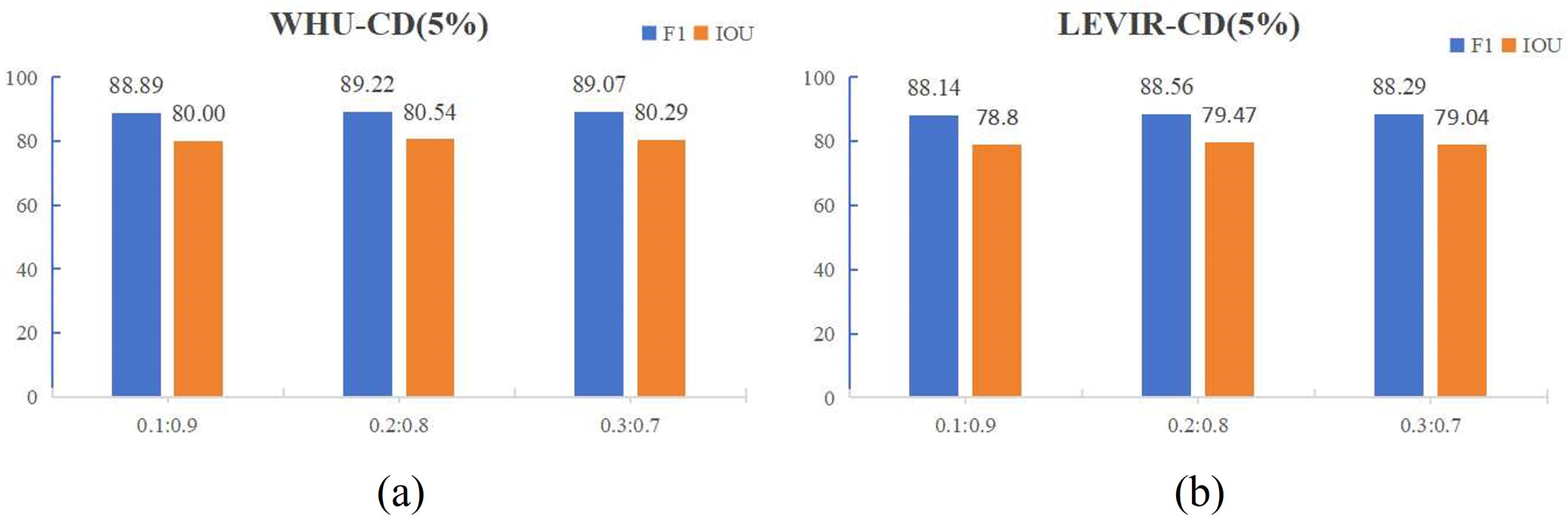
In the final part of the model, the effects of various perturbation patterns on training are examined through the loss functions utilized in both the jointly supervised ($L_s$) and the unsupervised ($L_u$) phases. Specifically,

Table 6. The use of loss functions for each part of the WHU-CD dataset.

Loss Function				WHU-5%
ID	$L_{sup}$	$L_{fp}$	$L_{sp}$	F1	IOU
A	✓			84.86	73.70
B	✓	✓		87.77	78.20
C	✓		✓	88.50	79.37
D	✓	✓	✓	88.51	79.39

presents the training results corresponding to different combinations of loss functions, while Figure 12 illustrates the effect of weights in unsupervised loss (see Equation (15)). A synthesis of the quantitative results from Figure 12 and Table 6 indicates that the overall performance of the model is improved with joint supervised and unsupervised loss functions. Notably, the most significant performance improvement is observed when the weights for $L_{fp}$ and $L_{sp}$ in the unsupervised loss are set to 0.8 and 0.2, respectively. Under these conditions, the F1 and IOU are improved by 4.36% and 6.84% in the WHU-CD, while improvements of 3.56% and 5.52% in the LEVIR-CD. This indicates that leveraging a limited amount of labeled data to acquire a priori knowledge, coupled with extensive knowledge mining from a substantial volume of unlabeled data, can significantly enhance model performance. This learning paradigm allows the model to achieve considerable performance gains with minimal reliance on labeled data, thereby improving its ability to detect changes in buildings in images and substantially reducing the demand for labeled data.

4.4.2. Selection and Use of Features

The gradual downsampling in the encoding–decoding network structure results in a loss of spatial information, and previous methods are insufficient for generating change features using only deep semantic features. To capture the advantages of change features across different scales, MSGF-Semi performs multi-feature fusion to capture both spatial and semantic information about change features at various scales, which generates more accurate representations of change features, thereby mitigating the inadequacy of pseudo-labels to express in areas of high uncertainty at the edges of buildings. To verify the effectiveness, we denote the encoder-generated features with distinct spatial structures as l1, l2, l3, and l4. Subsequently, we conducted experiments to validate the effectiveness of multi-feature fusion, encompassing a total of five experiments aimed at assessing the impact of feature fusion at different scales on model performance. The results, presented in

Table 7. Results for different feature layers using the encoder (5% in WHU-CD).

Feature Layers	F1	IOU	P	R
l3	87.98	78.54	88.23	87.73
l4	88.23	78.94	91.56	85.14
l1, l2, l3	88.75	79.77	90.34	87.20
l2, l3, l4	88.57	79.49	90.15	87.05
l1, l2, l3, l4	89.22	80.54	91.16	87.36

, indicate that the fusion of full-scale features yields significant performance improvements compared to the use of single-scale features, with F1 and IOU metrics increasing by 1.24% and 2.0%, respectively. This indicates that the use of multi-level features enhances the detailed representation of change features and allows the model to make more accurate determinations of low confidence areas, thus improving the recognition of change buildings.

4.4.3. Feature Visualization

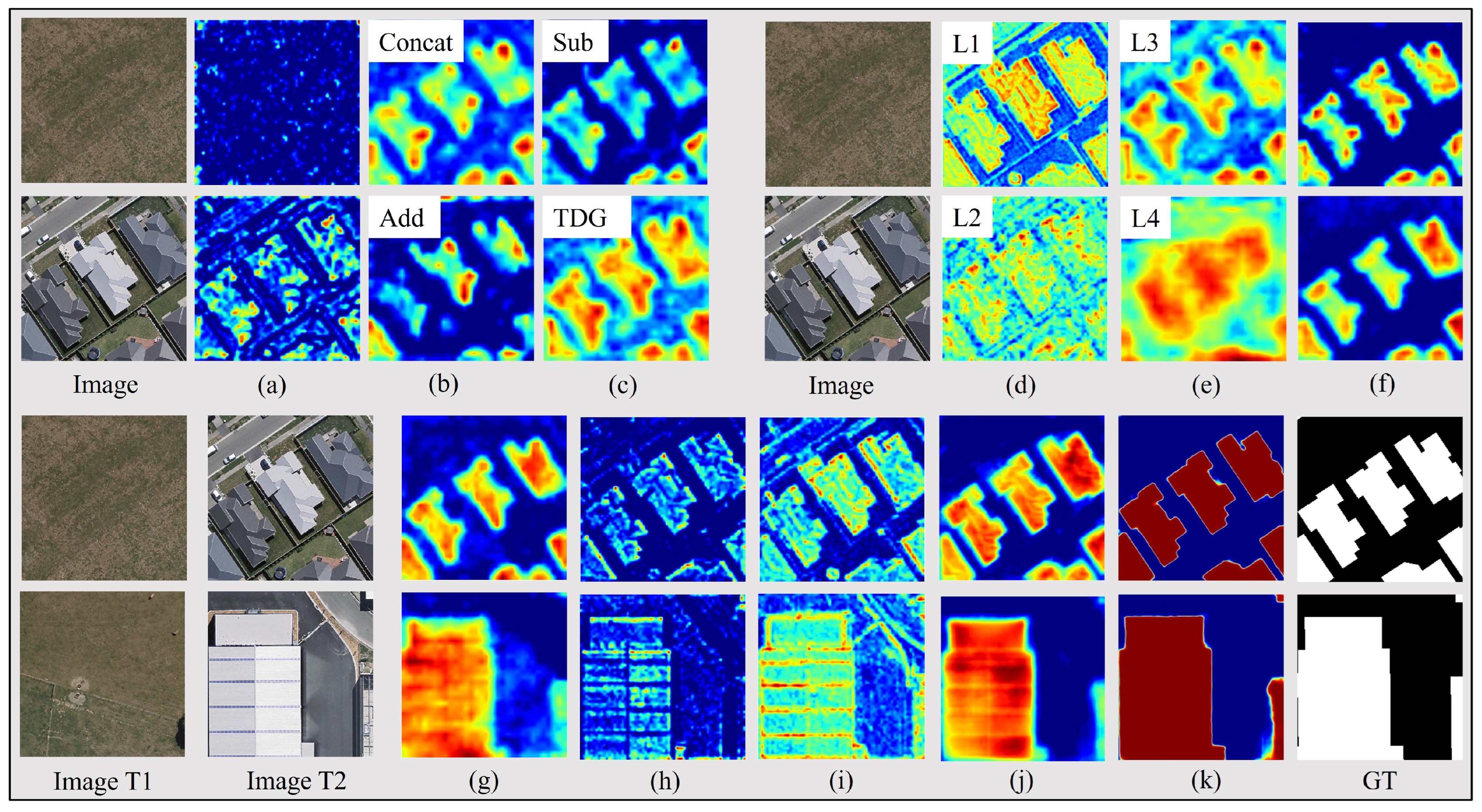
To better understand each module in the model, we provide visualization results of feature layers. In Figure 13, the Siamese encoder generates high-level feature maps $F_i$ (Figure 13a) for the images. Subsequently, change feature maps between image pairs are obtained, with Figure 13b,c showing the visualization results of change maps acquired through different methods. Specifically, Concat represents the channel-wise concatenation feature, Add represents the element-wise addition feature, Sub represents the element-wise subtraction feature, and TDG is the change feature generation method utilized in this study. The first three change feature generation methods have distinct advantages but may not fully capture changes, while the method proposed in this study effectively combines the strengths of these methods to highlight semantic regions related to changes. Subsequently, to better integrate multi-scale features, we introduce the FSF module in the feature fusion stage Figure 13d–f displays the visualization results, where L1, L2, L3, and L4 denote change feature maps from shallow to deep layers of the bitemporal image. Figure 13f represents the output after multi-level feature fusion and semantic enhancement. As displayed, features under different levels contain different amounts of information and are interfered with by other noisy information in addition to highlighting change buildings. The FSF module enables the fused feature maps to focus on the representation of foreground targets. On this basis, to improve the model’s ability to perceive change buildings in edge details, we designed the DSG module. The implementation of this module is shown in Figure 13g–j. Figure 13g represents deep features after semantic enhancement, Figure 13h represents the features after edge enhancement, Figure 13i represents shallow features, and Figure 13j represents the feature maps obtained after the DSG module. Additionally, Figure 13k represents change probability maps after threshold filtering. By combining the localization ability of deep semantic features with the detailed representation of shallow features via the DSG module, the resulting feature map can accurately represent the change buildings, making the final result closer to the real change and thus generating high-confidence pseudo-labels.

5. Conclusions

SSCD proposes better utilizing large amounts of unlabeled data. However, previous SSCD methods have traditionally focused on training strategies such as generative adversarial techniques and consistency regularization, often overlooking the effective utilization of multi-scale features. Consequently, the recognition outcomes of these methods are vulnerable to inherent biases and limitations in model design. In this research, we introduce a novel feature-extraction network named MSFGNet, built upon consistent regularization and pseudo-labeling. Our approach enhances the recognition performance of semi-supervised models by incorporating three main modules: TDG, FSF, and DSG. The TDG module dynamically extracts change features from diverse perspectives to enhance the model’s ability to detect change targets. The FSF module captures various change targets across multiple scales, leveraging the beneficial information within multi-scale features to produce more concise semantic representations of changes. Additionally, the DSG module facilitates learning shallow features and the fusion of different features to improve the model’s localization of change targets and the recognition of edge details. Experimental results on two standard datasets demonstrate that our method effectively leverages unlabeled data to bolster model learning and enhance the model’s capacity to identify changing buildings. Nevertheless, there is room for improvement in assessing pseudo-label reliability and the model’s information extraction capabilities. Future research directions could explore integrating traditional techniques with deep learning methods to identify high-confidence samples for model training and extend visual foundation models (VFMs) to leverage large-scale model learning combined with fine-tuning for domain-specific zero- or few-shot tasks. The development of these methods opens up new perspectives for model training with limited label availability.

References

1. Singh, A. Review article digital change detection techniques using remotely-sensed data. Int. J. Remote Sens. 1989, 10, 989–1003. [Google Scholar] [CrossRef]
2. Wen, D.; Huang, X.; Bovolo, F.; Li, J.; Ke, X.; Zhang, A.; Benediktsson, J.A. Change detection from very-high-spatial-resolution optical remote sensing images: Methods, applications, and future directions. IEEE Geosci. Remote Sens. Mag. 2021, 9, 68–101. [Google Scholar] [CrossRef]
3. Zhu, Q.; Guo, X.; Deng, W.; Shi, S.; Guan, Q.; Zhong, Y.; Zhang, L.; Li, D. Land-use/land-cover change detection based on a Siamese global learning framework for high spatial resolution remote sensing imagery. ISPRS J. Photogramm. Remote Sens. 2022, 184, 63–78. [Google Scholar] [CrossRef]
4. Jin, S.; Yang, L.; Danielson, P.; Homer, C.; Fry, J.; Xian, G. A comprehensive change detection method for updating the National Land Cover Database to circa 2011. Remote Sens. Environ. 2013, 132, 159–175. [Google Scholar] [CrossRef]
5. Huang, F.; Chen, L.; Yin, K.; Huang, J.; Gui, L. Object-oriented change detection and damage assessment using high-resolution remote sensing images, Tangjiao Landslide, Three Gorges Reservoir, China. Environ. Earth Sci. 2018, 77, 183. [Google Scholar] [CrossRef]
6. Zhang, C.; Yue, P.; Tapete, D.; Jiang, L.; Shangguan, B.; Huang, L.; Liu, G. A deeply supervised image fusion network for change detection in high resolution bi-temporal remote sensing images. ISPRS J. Photogramm. Remote Sens. 2020, 166, 183–200. [Google Scholar] [CrossRef]
7. Bruzzone, L.; Bovolo, F. A novel framework for the design of change-detection systems for very-high-resolution remote sensing images. Proc. IEEE 2012, 101, 609–630. [Google Scholar] [CrossRef]
8. Bruzzone, L.; Prieto, D.F. Automatic analysis of the difference image for unsupervised change detection. IEEE Trans. Geosci. Remote Sens. 2000, 38, 1171–1182. [Google Scholar] [CrossRef]
9. Zhang, Y.; Peng, D.; Huang, X. Object-based change detection for VHR images based on multiscale uncertainty analysis. IEEE Geosci. Remote Sens. Lett. 2017, 15, 13–17. [Google Scholar] [CrossRef]
10. Bruzzone, L.; Cossu, R.; Vernazza, G. Detection of land-cover transitions by combining multidate classifiers. Pattern Recognit. Lett. 2004, 25, 1491–1500. [Google Scholar] [CrossRef]
11. Ertürk, A.; Iordache, M.D.; Plaza, A. Sparse unmixing-based change detection for multitemporal hyperspectral images. IEEE J. Sel. Top. Appl. Earth Obs. Remote Sens. 2015, 9, 708–719. [Google Scholar] [CrossRef]
12. Deng, J.; Wang, K.; Deng, Y.; Qi, G. PCA-based land-use change detection and analysis using multitemporal and multisensor satellite data. Int. J. Remote Sens. 2008, 29, 4823–4838. [Google Scholar] [CrossRef]
13. Alcantarilla, P.F.; Stent, S.; Ros, G.; Arroyo, R.; Gherardi, R. Street-view change detection with deconvolutional networks. Auton. Robot. 2018, 42, 1301–1322. [Google Scholar] [CrossRef]
14. Daudt, R.C.; Le Saux, B.; Boulch, A. Fully convolutional siamese networks for change detection. In Proceedings of the 25th IEEE International Conference on Image Processing (ICIP), Athens, Greece, 7–10 October 2018; pp. 4063–4067. [Google Scholar]
15. Chen, Z.; Zhou, Y.; Wang, B.; Xu, X.; He, N.; Jin, S.; Jin, S. EGDE-Net: A building change detection method for high-resolution remote sensing imagery based on edge guidance and differential enhancement. ISPRS J. Photogramm. Remote Sens. 2022, 191, 203–222. [Google Scholar] [CrossRef]
16. Zhang, C.; Wang, L.; Cheng, S.; Li, Y. SwinSUNet: Pure transformer network for remote sensing image change detection. IEEE Trans. Geosci. Remote Sens. 2022, 60, 5224713. [Google Scholar] [CrossRef]
17. Xia, L.; Chen, J.; Luo, J.; Zhang, J.; Yang, D.; Shen, Z. Building change detection based on an edge-guided convolutional neural network combined with a transformer. Remote Sens. 2022, 14, 4524. [Google Scholar] [CrossRef]
18. Chen, H.; Qi, Z.; Shi, Z. Remote sensing image change detection with transformers. IEEE Trans. Geosci. Remote Sens. 2021, 60, 5607514. [Google Scholar] [CrossRef]
19. Wang, L.; Li, H. Hmcnet: Hybrid efficient remote sensing images change detection network based on cross-axis attention mlp and cnn. IEEE Trans. Geosci. Remote Sens. 2022, 60, 5236514. [Google Scholar] [CrossRef]
20. Song, X.; Hua, Z.; Li, J. Remote sensing image change detection transformer network based on dual-feature mixed attention. IEEE Trans. Geosci. Remote Sens. 2022, 60, 5920416. [Google Scholar] [CrossRef]
21. Chen, H.; Shi, Z. A spatial-temporal attention-based method and a new dataset for remote sensing image change detection. Remote Sens. 2020, 12, 1662. [Google Scholar] [CrossRef]
22. Fang, S.; Li, K.; Shao, J.; Li, Z. SNUNet-CD: A densely connected Siamese network for change detection of VHR images. IEEE Geosci. Remote Sens. Lett. 2021, 19, 8007805. [Google Scholar] [CrossRef]
23. Yang, L.; Zhuo, W.; Qi, L.; Shi, Y.; Gao, Y. St++: Make self-training work better for semi-supervised semantic segmentation. In Proceedings of the IEEE/CVF Conference on Computer Vision and Pattern Recognition, New Orleans, LA, USA, 18–24 June 2022; pp. 4268–4277. [Google Scholar]
24. Feng, Z.; Zhou, Q.; Gu, Q.; Tan, X.; Cheng, G.; Lu, X.; Shi, J.; Ma, L. Dmt: Dynamic mutual training for semi-supervised learning. Pattern Recognit. 2022, 130, 108777. [Google Scholar] [CrossRef]
25. Gong, M.; Yang, Y.; Zhan, T.; Niu, X.; Li, S. A generative discriminatory classified network for change detection in multispectral imagery. IEEE J. Sel. Top. Appl. Earth Obs. Remote Sens. 2019, 12, 321–333. [Google Scholar] [CrossRef]
26. Sohn, K.; Berthelot, D.; Carlini, N.; Zhang, Z.; Zhang, H.; Raffel, C.A.; Cubuk, E.D.; Kurakin, A.; Li, C.L. Fixmatch: Simplifying semi-supervised learning with consistency and confidence. Adv. Neural Inf. Process. Syst. 2020, 33, 596–608. [Google Scholar]
27. Ouali, Y.; Hudelot, C.; Tami, M. Semi-supervised semantic segmentation with cross-consistency training. In Proceedings of the IEEE/CVF Conference on Computer Vision and Pattern Recognition, Seattle, WA, USA, 13–19 June 2020; pp. 12674–12684. [Google Scholar]
28. Wang, L.; Zhang, M.; Shi, W. STCRNet: A Semi-Supervised Network Based on Self-Training and Consistency Regularization for Change Detection in VHR Remote Sensing Images. IEEE J. Sel. Top. Appl. Earth Obs. Remote Sens. 2023, 17, 2272–2282. [Google Scholar] [CrossRef]
29. Wang, J.X.; Li, T.; Chen, S.B.; Tang, J.; Luo, B.; Wilson, R.C. Reliable contrastive learning for semi-supervised change detection in remote sensing images. IEEE Trans. Geosci. Remote Sens. 2022, 60, 4416413. [Google Scholar] [CrossRef]
30. Peng, D.; Bruzzone, L.; Zhang, Y.; Guan, H.; Ding, H.; Huang, X. SemiCDNet: A semisupervised convolutional neural network for change detection in high resolution remote-sensing images. IEEE Trans. Geosci. Remote Sens. 2020, 59, 5891–5906. [Google Scholar] [CrossRef]
31. Zhang, X.; Huang, X.; Li, J. Semisupervised change detection with feature-prediction alignment. IEEE Trans. Geosci. Remote Sens. 2023, 61, 5401016. [Google Scholar] [CrossRef]
32. Bandara, W.G.C.; Patel, V.M. Revisiting consistency regularization for semi-supervised change detection in remote sensing images. arXiv 2022, arXiv:2204.08454. [Google Scholar]
33. Sun, C.; Wu, J.; Chen, H.; Du, C. SemiSANet: A semi-supervised high-resolution remote sensing image change detection model using Siamese networks with graph attention. Remote Sens. 2022, 14, 2801. [Google Scholar] [CrossRef]
34. Yang, L.; Qi, L.; Feng, L.; Zhang, W.; Shi, Y. Revisiting weak-to-strong consistency in semi-supervised semantic segmentation. In Proceedings of the IEEE/CVF Conference on Computer Vision and Pattern Recognition, Vancouver, BC, Canada, 17–24 June 2023; pp. 7236–7246. [Google Scholar]
35. Ji, S.; Wei, S.; Lu, M. Fully convolutional networks for multisource building extraction from an open aerial and satellite imagery data set. IEEE Trans. Geosci. Remote Sens. 2018, 57, 574–586. [Google Scholar] [CrossRef]
36. Laine, S.; Aila, T. Temporal ensembling for semi-supervised learning. arXiv 2016, arXiv:1610.02242. [Google Scholar]
37. Tarvainen, A.; Valpola, H. Mean teachers are better role models: Weight-averaged consistency targets improve semi-supervised deep learning results. In Proceedings of the Advances in Neural Information Processing Systems, Long Beach, CA, USA, 4–9 December 2017; Volume 30. [Google Scholar]
38. Wang, J.X.; Chen, S.B.; Ding, C.H.; Tang, J.; Luo, B. RanPaste: Paste consistency and pseudo-label for semisupervised remote sensing image semantic segmentation. IEEE Trans. Geosci. Remote Sens. 2021, 60, 2002916. [Google Scholar] [CrossRef]
39. Cubuk, E.D.; Zoph, B.; Mane, D.; Vasudevan, V.; Le, Q.V. Autoaugment: Learning augmentation policies from data. arXiv 2018, arXiv:1805.09501. [Google Scholar]
40. Cubuk, E.D.; Zoph, B.; Shlens, J.; Le, Q.V. Randaugment: Practical automated data augmentation with a reduced search space. In Proceedings of the IEEE/CVF Conference on Computer Vision and Pattern Recognition Workshops, Seattle, WA, USA, 14–19 June 2020; pp. 702–703. [Google Scholar]
41. Xie, Q.; Dai, Z.; Hovy, E.; Luong, T.; Le, Q. Unsupervised data augmentation for consistency training. Adv. Neural Inf. Process. Syst. 2020, 33, 6256–6268. [Google Scholar]
42. Chen, X.; Yuan, Y.; Zeng, G.; Wang, J. Semi-supervised semantic segmentation with cross pseudo supervision. In Proceedings of the IEEE/CVF Conference on Computer Vision and Pattern Recognition, Nashville, TN, USA, 20–25 June 2021; pp. 2613–2622. [Google Scholar]
43. Zhang, X.; Huang, X.; Li, J. Joint self-training and rebalanced consistency learning for semi-supervised change detection. IEEE Trans. Geosci. Remote Sens. 2023, 61, 5406613. [Google Scholar] [CrossRef]
44. Shu, Q.; Pan, J.; Zhang, Z.; Wang, M. MTCNet: Multitask consistency network with single temporal supervision for semi-supervised building change detection. Int. J. Appl. Earth Obs. Geoinf. 2022, 115, 103110. [Google Scholar] [CrossRef]
45. Yun, S.; Han, D.; Oh, S.J.; Chun, S.; Choe, J.; Yoo, Y. Cutmix: Regularization strategy to train strong classifiers with localizable features. In Proceedings of the IEEE/CVF International Conference on Computer Vision, Seoul, Republic of Korea, 27 October–2 November 2019; pp. 6023–6032. [Google Scholar]
46. He, K.; Zhang, X.; Ren, S.; Sun, J. Deep residual learning for image recognition. In Proceedings of the IEEE Conference on Computer Vision and Pattern Recognition, Las Vegas, NV, USA, 27–30 June 2016; pp. 770–778. [Google Scholar]
47. Mittal, S.; Tatarchenko, M.; Brox, T. Semi-supervised semantic segmentation with high-and low-level consistency. IEEE Trans. Pattern Anal. Mach. Intell. 2019, 43, 1369–1379. [Google Scholar] [CrossRef]
48. Vu, T.H.; Jain, H.; Bucher, M.; Cord, M.; Pérez, P. Advent: Adversarial entropy minimization for domain adaptation in semantic segmentation. In Proceedings of the IEEE/CVF Conference on Computer Vision and Pattern Recognition, Long Beach, CA, USA, 15–20 June 2019; pp. 2517–2526. [Google Scholar]
Figure 1. Examples of low-quality pseudo-label when there are pseudo-changes and a small number of labels available.
Remotesensing 16 03424 g001
Figure 2. Diagram of the method. (a) denotes the supervised stage. (b) denotes the unsupervised stage.
Remotesensing 16 03424 g002
Figure 3. Unlabeled data input perturbation flowchart. Where the red box shows the result after the random mix-mask operation.
Remotesensing 16 03424 g003
Figure 4. Network framework diagram. The network structure consists of the encoder, an adaptive change feature perceptions module, and a Decoder part. The two-branch encoder consists of four residual blocks of ResNet-18. The adaptive difference feature learning module consists of four TDG modules. The decoder consists of the full-scale feature fusion module and the deep semantic guidance module.
Remotesensing 16 03424 g004
Figure 5. Adaptive difference feature learning module.
Remotesensing 16 03424 g005
Figure 6. Multiscale feature fusion and guidance module.
Remotesensing 16 03424 g006
Figure 7. Visualization results of different semi-supervised methods at a 5% labeling rate in WHU-CD dataset.
Remotesensing 16 03424 g007
Figure 8. Visualization results of MSFGNet under different labeling rates in the WHU-CD dataset.
Remotesensing 16 03424 g008
Figure 9. Visualization results of different semi-supervised methods at a 5% labeling rate in the LEVIR-CD dataset.
Remotesensing 16 03424 g009
Figure 10. Visualization results of MSFGNet under different labeling rates in the LEVIR-CD dataset.
Remotesensing 16 03424 g010
Figure 11. Visualization results of the ablation experiments.
Remotesensing 16 03424 g011
Figure 12. Experimental results of unsupervised loss function participation weights for each part. (a) Training results in WHU-CD at 5% data; (b) Training results in LEVIR-CD at 5% data.
Remotesensing 16 03424 g012
Figure 13. Feature visualization. (a) Initial features of image pairs. (b,c) are change features. (d,e) are different levels of change feature. (f) Output of the FSF module. (gi) Three inputs of the DSG module. (j) Output of the DSG module. (k) Change probability map, where red indicates higher attention values and blue indicates lower attention values.
Remotesensing 16 03424 g013