Article

Evaluation of the Surface Downward Longwave Radiation Estimation Models over Land Surface

by
Yingping Chen
1,2,
Bo Jiang
1,2,*,
Jianghai Peng
3,
Xiuwan Yin
1,2 and
Yu Zhao
1,2
1
State Key Laboratory of Remote Sensing Science, Faculty of Geographical Science, Beijing Normal University, Beijing 100875, China
2
Beijing Engineering Research Center for Global Land Remote Sensing Products, Faculty of Geographical Science, Beijing Normal University, Beijing 100875, China
3
Center for Global Discovery and Conservation Science, School of Earth and Space Exploration, Arizona State University, Tempe, AZ 85281, USA
*
Author to whom correspondence should be addressed.
Remote Sens. 2024, 16(18), 3422; https://doi.org/10.3390/rs16183422
Submission received: 31 July 2024 / Revised: 31 August 2024 / Accepted: 12 September 2024 / Published: 14 September 2024
(This article belongs to the Special Issue Earth Radiation Budget and Earth Energy Imbalance)

Abstract

:
Surface downward longwave radiation (SDLR) is crucial for maintaining the global radiative budget balance. Due to their ease of practicality, SDLR parameterization models are widely used, making their objective evaluation essential. In this study, against comprehensive ground measurements collected from more than 300 globally distributed sites, four SDLR parameterization models, including three popular existing ones and a newly proposed model, were evaluated under clear- and cloudy-sky conditions at hourly (daytime and nighttime) and daily scales, respectively. The validation results indicated that the new model, namely the Peng model, originally proposed for SDLR estimation at the sea surface and applied for the first time to the land surface, outperformed all three existing models in nearly all cases, especially under cloudy-sky conditions. Moreover, the Peng model demonstrated robustness across various land cover types, elevation zones, and seasons. All four SDLR models outperformed the Global Land Surface Satellite product from Advanced Very High-Resolution Radiometer Data (GLASS-AVHRR), ERA5, and CERES_SYN1de-g_Ed4A products. The Peng model achieved the highest accuracy, with validated RMSE values of 13.552 and 14.055 W/m2 and biases of −0.25 and −0.025 W/m2 under clear- and cloudy-sky conditions at daily scale, respectively. Its superior performance can be attributed to the inclusion of two cloud parameters, total column cloud liquid water and ice water, besides the cloud fraction. However, the optimal combination of these three parameters may vary depending on specific cases. In addition, all SDLR models require improvements for wetlands, bare soil, ice-covered surfaces, and high-elevation regions. Overall, the Peng model demonstrates significant potential for widespread use in SDLR estimation for both land and sea surfaces.

1. Introduction

Surface downward longwave radiation (SDLR) refers to the thermal radiation, with wavelength ranging from 4 to 100 μ m , emitted by atmospheric constituents such as H 2 O , CO 2 , O 3 molecules, and cloud water droplets near the Earth’s surface. As a fundamental component of the surface radiation budget [1], studying SDLR is crucial for understanding the energy exchange between the Earth’s surface and the atmosphere. SDLR also plays a pivotal role in climate dynamics, weather forecasts, agricultural practices, and other studies and applications [2,3].
Although SDLR measurements are generally considered accurate, there remains a significant need for precise SDLR estimation methods due to limitations, such as poor spatial representativeness, uneven spatial distribution, and short duration of ground-based measurements [4,5]. Therefore, numerous SDLR estimation models have been successfully proposed. These widely used SDLR estimation models can be roughly categorized into four types: physical models, hybrid models, machine learning models, and parameterization models. Physical models, such as radiative transfer models, calculate SDLR by accounting for interactions between the Earth’s surface and the atmosphere, along with extensive meteorological and surface information. Most of the classic remotely sensed SDLR products were generated from these models, such as the International Satellite Cloud Climatology Project (ISCCP) [6]. However, physical models are often complex, and obtaining the necessary inputs is challenging. Hybrid models combine physical models with statistical methods, resulting in higher computational efficiency and a well-defined physical foundation. The newly released SDLR product from the Moderate-resolution Imaging Spectroradiometer (MODIS) data collected in the Global Land Surface Satellite (GLASS) suite product (namely GLASS-MODIS) [7] under clear-sky conditions was generated using this type of model. However, hybrid models struggle with cloudy-sky conditions, as satellite observations alone cannot fully capture the thermal contributions from cloud layers and the underlying atmosphere [8,9]. Recent advances in machine learning have led to the successful application of various machine learning and deep learning methods for SDLR estimation [10,11] and even have been applied to generate a new SDLR product from the Advanced Very High-Resolution Radiometer (AVHRR) data collected in GLASS, known as GLASS-AVHRR [12]. Nonetheless, these approaches often involve substantial computational costs and complex model architectures.
Relatively, parameterization models, which are based on statistical relationships between SDLR and certain meteorological parameters, such as the near-surface air temperature (Ta, Unit: K), relative humidity (RH), cloud-related factors, and other ancillary information, are widely used due to their easy implementation, high computational efficiency, and satisfactory performance. Therefore, plenty of SDLR parameterization models have been proposed. Specifically, for clear-sky conditions, the SDLR parameterization models are typically extensions of the Stefan–Boltzmann law, assuming that the effects of atmospheric scattering can be neglected. This makes the determination of the atmospheric effective emissivity ( ε 0 ) essential. Previous studies have suggested that ε 0 is related to near-surface water vapor pressure (ea, Unit: hPa) [13,14], Ta [1,15], or both [16,17,18,19]. Meanwhile, for cloudy-sky conditions, the corresponding SDLR parameterization models usually combine clear-sky SDLR parameterization models with terms for cloud parameters, such as cloud cover [20] and cloud-base temperature (CBT) [21]. However, these cloud-related parameters are difficult to obtain, particularly CBT, which almost dominates the cloudy sky SDLR. Hence, some studies have proposed indirect methods to obtain CBT from other easily obtained parameters. For instance, CBT estimated from cloud thickness was used in a parameterization model to produce the GLASS-MODIS cloudy-sky SDLR product [8]. Recently, the total amount of liquid water per unit area in the air column from the base to the top of the cloud, called total column cloud liquid water (clw), and its chilled counterpart (ice), called total column cloud ice water (ciw), which are physically correlated with CBT through the cloud base height, were first introduced for estimating cloud-sky SDLR at sea surface to achieve better results [22]. Thus, the performance of parameterization models highly depends on the choice of parameters and the quality of the data used for model training.
Meanwhile, the evaluation of existing SDLR parameterization methods has attracted extensive attention. Early evaluations were often limited to specific geographic regions, leading to diverse and sometimes conflicting results. For instance, Kjaersgaard et al. [23] assessed twenty SDLR models at both daily and hourly scales against the measurements from two locations in Denmark. Their results indicated that models developed by Swinbank [15], Prata [17], and Brutsaert [16] performed well under clear-sky conditions but struggled to accurately estimate SDLR at lower values. However, studies conducted in northeastern and southern Brazil [4,24] questioned these findings. They suggested that SDLR parameterization models incorporating physical mechanisms, such as Brutsaert [16], generally performed better. Conversely, the models relying solely on Ta, such as Swinbank [15], tended to overestimate and exhibit lower accuracy. Afterward, more and more comprehensive in situ measurements were utilized to assess SDLR models with the establishment of globally distributed sites. For example, Guo et al. [25] and Cheng et al. [26] evaluated seven clear-sky and seven cloudy-sky SDLR parameterization models at instantaneous scale by using ground measurements from 71 and 44 globally distributed stations, respectively, and they recommended the model proposed by Carmona et al. [27]. Most of their findings were consistent with previous studies, and they further pointed out that the uncertainty of the SDLR parameterization models was mostly from terms relating to moisture (e.g., RH and water vapor) and cloud properties. Overall, it was suggested that incorporating more precise information about cloud and moisture, as well as physical mechanisms, could enhance the accuracy of SDLR parameterization models. Although these studies provided valuable insights for model developers and users, certain limitations remained. Firstly, due to the limitations of available in situ measurements, most evaluations only focused on the instantaneous scale, whereas the performance of SDLR models at a daily scale under all-sky conditions needs more attention [22]. Secondly, the robustness of these models globally, especially over the polar regions, has not been explored thoroughly. Additionally, new SDLR parameterization models for sea surface proposed by Peng et al. [22] in recent years, which is different from most of the previous models by taken into more cloud-related parameters account, has not been comprehensively assessed at land surface though it worked very well at sea surface.
Therefore, the primary objective of this study is to evaluate the performance of four SDLR parameterization models, including three widely used existing models and a new model developed by Peng et al. [22] (referred to as the Peng model), which was originally designed for ocean surface at both hourly and daily scales under clear- or/and cloudy-sky conditions globally. After that, further analysis of the Peng model was conducted under various conditions, including land cover type, elevation, and season. The paper is organized as follows: Section 2 introduces the four evaluated SDLR parameterization models; Section 3 details the data and methods used; and the model evaluation results and further analysis of the Peng model are provided in Section 4.

2. Materials

Table 1 lists all the variables used in this study and their sources. Two time scales, hourly and daily, were considered. Therefore, all variables were pre-processed to match these time scales. More details about these data are given below.

2.1. Ground Measurements

Ground measurements were collected from 318 sites across nine observational networks spanning from 1992 to 2021. Note that only the sites providing the five radiative and meteorological measurements, including DSR, USR, SDLR, Ta, and RH simultaneously, were selected in this study. Figure 1 illustrates the spatial distribution of these sites, which cover latitudes ranging from 89.98°S to 82.49°N and elevations ranging from 0 to 4318 m. The sites encompass eight main land cover types, including cropland (CRO, 39 sites), bare land (BSV, 6 sites), forest (FRO, 108 sites), grassland (GRA, 103 sites), ice (ICE, 23 sites), wetland (WET, 18 sites), shrubland (SHR, sites), and tundra (TUN, 2 sites). This diverse representation of land cover types, climatic zones, spatial distribution, and elevation ranges ensured a thorough evaluation of the four SDLR models.
To ensure data quality, all measurements with high quality defined by their providers were further examined manually to remove any unreasonable samples with abnormal values (i.e., extremely high or low). After converting into local time format, all measurements with a sampling frequency (see Table 2) of less than one hour were aggregated into hourly means, provided that 80% of the measurements within one hour were available. Subsequently, all hourly data were aggregated into daily means without any missing values. Afterward, two variables, Sn and ea, were calculated using these hourly/daily ground measurements. Specifically, Sn was computed by subtracting USR from DSR, and it was used to categorize all hourly samples into daytime or nighttime, with the hourly samples in the daytime if Sn > 20 W/m2 and vice versa, as suggested by Wang K et al. [36]. Whereas ea was calculated from RH using the following equation [25]:
e a = e s RH 100 = 6.108 exp 17.27 T a T a + 237.3 RH 100  
where e s is the saturation vapor pressure at a specific Ta. Note that the unit of Ta is in Equation (1).
Furthermore, all hourly/daily samples under clear skies were identified according to the corresponding hourly/daily clearness index (CI). CI is defined as the ratio of the DSR and the extraterrestrial radiation (DSRtoa) and is usually employed to measure the atmospheric transmittance and ascertain the sky conditions [37,38].
C I = D S R D S R t o a
In this study, the hourly and daily CI were both used. As per previous studies [22,39], if the hourly or daily CI > 0.7, then it indicates the hourly or daily under clear sky conditions, and CI ≤ 0.7 indicates under a cloudy sky. The hourly CI was calculated by Equation (2) with hourly DSR measurements and hourly DSRtoa_hourly computed by [40]:
D S R t o a _ h o u r l y = 12 π G S C d r sin φ cos δ ( sin ω 2 sin ω 1 ) + π ω 2 ω 1 180 sin φ sin δ
δ = 0.409   sin 2 π d o y 365 1.39
d r = 1 + 0.033 cos 2 π d o y 365
where G S C is the solar constant (1367 W/m2); φ and δ are the latitude (unit: rad) and solar declination angle (unit: rad), respectively; doy is the day of the year; and d r is the inverse relative distance from the Earth to the Sun; ω1 and ω2 are the hour angles (unit: degrees) at the beginning and the end of the hour interval. Note that the nighttime CI was computed using the method suggested by Flerchinger et al. [41], which involves a 24 h solar radiation window centered around each hourly observation.
The daily CI was calculated by Equation (2) with daily DSR measurements and daily DSRtoa_daily computed by [42]:
D S R t o a _ d a i l y = 1440 π G s c d r ω s sin φ cos δ + cos δ sin ω s
ω s = c o s 1 tan φ tan δ
where G s c is the solar constant (0.0820 MJm−2 min−1); ω s is the sunset hour angle (unit: rad).
Therefore, there were 10,312,034 samples (2,459,204 under clear-sky conditions and 7,852,830 under cloudy-sky conditions) at hourly scale, and 601,331 samples (131,745 under clear-sky conditions and 469,586 under cloudy-sky conditions) at daily scale used for evaluation, respectively.
To ensure a thorough evaluation, six cases (cases1–6) were considered, corresponding to hourly daytime/nighttime and daily under clear-sky conditions and hourly daytime/nighttime and daily under cloudy-sky conditions, respectively. In each case, all models were first trained with these samples. Finally, in each case, 70% of the samples at each site were randomly selected for model training, and the remaining 30% were used for independent validation. The size of each sample dataset is listed in Table 3.

2.2. ERA5 Reanalysis Meteorological Data

ERA5 (https://cds.climate.copernicus.eu/cdsapp#!/home, accessed on 11 September 2024), produced by the European Centre for Medium-Range Weather Forecasts (ECMWF), is the fifth-generation atmospheric reanalysis dataset [43]. Covering the period from 1970 to the present, ERA5 provides a comprehensive record of global climate and weather. It integrates model simulations with global observations through 4D-Var data assimilation within the Integrated Forecasting System (IFS), achieving an enhanced spatial resolution of 0.25° and a temporal resolution of hourly intervals compared to ERA-interim [44]. Although existing studies have demonstrated the satisfactory accuracy of ERA5 at the monthly average scale [45], specialized validation studies for cloud-related parameters (C, clw, and ciw) at the hourly or daily scale are still lacking. Despite this, ERA5 remains a valuable data source, particularly given the absence of other similarly high-resolution alternatives for hourly-scale cloud parameters. We believe that ERA5 remains a valuable data source, especially in the absence of other similarly high-resolution alternatives. For this study, the three hourly cloud-related parameters (C, clw, and ciw) were extracted from ERA5 for 318 stations spanning from 1992 to 2021 and aggregated into daily averages. Additionally, ERA5 SDLR data at both hourly and daily scales, derived from the RRTM fast radiative transfer model, were also obtained for inter-comparison because of its slightly superior performance compared to CERES [46].

2.3. Remotely Sensed SDLR Products

Two remotely sensed SDLR products, CERES SYN1-deg_Ed4A (CERES4 for short) and GLASS-AVHRR, were used for comparison in this study.
  • CERES4: The CERES SYN1deg_Ed4A product (https://ceres.larc.nasa.gov/, accessed on 11 September 2024) provides global surface radiative flux data with a 1-degree spatial resolution at hourly and daily scales since 2000 [47]. SDLR values are derived from the Langley Fu-Liou radiative transfer model by incorporating the inputs from MODIS, geostationary satellites (GEO), and meteorological profile data from GEOS-4 and GEOS-5 [48,49,50]. Xu et al. [51] conducted a validation using ground measurements from 288 sites to evaluate three satellite products (GLASS-MODIS V40, GLASS-AVHRR, and CERES-SYN) and three reanalysis datasets (ERA5, MERRA-2, and GLDAS). The results indicated that SDLR values from GLASS-AVHRR, CERES-SYN, and ERA5 exhibited higher accuracy compared to the other three products, with CERES4 demonstrating a bias of −1.54 W/m2 and an RMSE of 22.49 W/m2 at the daily scale. For this study, CERES4 hourly and daily SDLR data were extracted for the 319 sites.
  • GLASS-AVHRR: GLASS-AVHRR (https://glass-product.bnu.edu.cn/, accessed on 11 September 2024) provides global daily all-sky SDLR data from 1981 to 2021 with a spatial resolution of 5 km. It utilizes a densely connected convolutional neural network (DesCNN) and a transfer learning strategy to derive SDLR from AVHRR TOA bands and ERA5 near-surface meteorological parameters (i.e., Ta, ea, and RH). The product has been rigorously validated across 231 globally distributed sites, with an all-sky RMSE of 18.66 W / m 2 and a mean bias error of −2.69 W / m 2 . Moreover, Xu et al. [51] also demonstrated that estimates from GLASS-AVHRR and the ERA5 SDLR product were more accurate and stable compared to other products (e.g., GLASS-MODIS). Like CERES4, the GLASS-AVHRR SDLR was also extracted, but only at the daily scale.
Ultimately, the common samples were screened for inter-comparison between all four models and the three SDLR products. After matching, there were 708,880 and 2,251,078 common hourly samples under clear-sky and cloudy-sky conditions and 33,985 and 121,165 common daily samples under clear-sky and cloudy-sky, respectively.

3. Methods

3.1. Brief Review of the Four Evaluated SDLR Parameterization Models

The four evaluated SDLR parameterization models include three existing models, namely the Prata model [17], which only works under clear-sky conditions; the K-C model [27,52], designed for cloudy-sky conditions; and the Carmona2 model [27], applicable to all-sky conditions; as well as the newly developed Peng model [22], which also works for all-sky conditions. The three existing models were thought to have superior performance, and this study marks the first time the Peng model has been applied to land surface. Detailed descriptions of the four models are provided below.
  • Prata Model
The Prata model was proposed based on a new emissivity model, which was also proposed by Prata [17] under the assumption that the overall longwave spectrum under clear-sky conditions could be represented by a modified exponential band model that combines Ta and ea. Consequently, the Prata model can only be used for clear-sky SDLR estimation. It is expressed as follows:
SDLR = 1 1 + 46.5 e a T a exp a 1 + b 1 46.5 e a T a 0.5 σ T a 4
where σ is the Stefan–Boltzmann constant ( 5.67 × 10 8   Wm 2 K 4 ), and a1 and b1 are empirical coefficients defined as 1.2 and 3 in the original study, and they were obtained through the modeled clear-sky emissivity at various water vapor path lengths provided by Robinson [53,54]. Based on clear-sky SDLR measurements (No. of samples = 14) from a site near Hay in New South Wales, Australia, and data from various published sources (No. of samples = 254), the authors validated the Prata model and compared it with five other commonly used models. The results showed that the performance of the Prata model was equal to or even better than the other five models in all cases, especially in the polar, mid-latitude, or tropical regions. Afterward, Flerchinger et al. [41] also highlighted the Prata model’s high estimation accuracy after evaluating 13 clear-sky SDLR models at 14 sites in North America and China. Similar conclusions were also drawn by Guo et al. [25] on a global scale. Moreover, Guo et al. [25] found that the performance of the Prata model changed little, even with its original coefficients, when used globally because of its physical mechanism. However, several studies have also indicated that the Prata model with original coefficients tends to overestimate SDLR [4,24,27]. Additionally, like the Carmona2 model and others, its accuracy diminishes when applied to forest, wetland, and ice surfaces [25].
B.
Carmona2 Model
The Carmona2 model is an update of the SDLR estimation models developed by Carmona et al. [27]. This model was built based on 8393 daytime measurements from eight measuring campaigns in Argentina [55], and it can work under all-sky conditions at an hourly scale. The Carmona2 model uses a multivariate linear regression format, mathematically expressed as:
SDLR = a 2 + b 2 T a + d 2 RH + e 2 C σ T a 4
where C is the cloud fraction (0~1, dimensionless), and a2, b2, d2, and e2 are the empirical coefficients defined as −0.34, 3.36 × 10 3 , 1.94 × 10 3 , and 0.213 in the original study, respectively.
According to previous studies [25,26], under clear-sky conditions (C = 0 in Equation (9)), the Carmona2 model and its earlier version (referred to as the Carmona model) performed the best at instantaneous scale compared to other models due to their similar formats. Under cloudy skies, the Carmona2 model showed superior performance. Hence, the Carmona2 model was selected for evaluation in this study. However, it has limitations, such as reduced accuracy in high-altitude regions and coefficients that are constrained by specific geographical locations and atmospheric conditions.
C.
K-C Model
Distinct from the other three evaluated models, the K-C model combines two SDLR parameterization models, one developed by Thomas Konzelmann et al. [52] for cloudy-sky conditions (referred to as the K model) and a simplified version of the Carmona model only for clear-sky conditions [27]. The K model (see Equation (10)) was built based on measurements from seven sites in three meteorological experimental areas with different elevations in western Greenland, applicable to both instantaneous and daily scales. In the K model, the emissivity is considered to be the weighted average of clear-sky and overcast-sky emissivity values.
SDLR = SDLR clr 1 + C e 3 + f 3 C e 3 σ T a 4
where the empirical coefficients e3 and f3 were defined as 0.963 and 3 for daily scales and 0.952 and 4 for instantaneous scales, respectively. SDLRclr is the corresponding SDLR under clear-sky conditions, which can be estimated from the simplified Carmona model Equation (9) as suggested by Cheng et al. [26] for its satisfactory performance both regionally and globally.
SDLR = a 3 + b 3 T a + d 3 RH σ T a 4
where the empirical coefficients a3, b3, and d3 were defined as −0.34, 3.36 × 10 3 , and 1.94 × 10 3 in the original study. According to Cheng et al. [26], the performance of the K-C model ranked second to the Carmona2 model under cloudy-sky conditions. Like other models, it underestimated the SDLR over bare land and forest while tending to overestimate the SDLR over grassland.
D.
Peng Model
As mentioned above, the Peng model [22] was proposed for the all-sky SDLR estimation at the ocean surface for both hourly and daily scales. This model was built based on comprehensive measurements collected from 65 moored buoys distributed across global seas from 1988 to 2019. The Peng model is formulated as a nonlinear function of Ta, RH, C, clw (Unit: g / m 2 ), and ciw (Unit: g / m 2 ), as follows:
SDLR = a 4 T a 4 + b 4 C + d 4 ln 1 + clw + e 4 ln 1 + ciw + f 4 RH + g 4
where a4, b4, d4, e4, f4, and g4 are the empirical coefficients. And their empirical values are 1.06, 42.18, 4.90, −1.97, 0.89, and −178.28, respectively. After validation against the moored buoy measurements and inter-comparison with other existing models, the authors claimed that the Peng model outperformed the other models at both hourly (daytime and nighttime) and daily scales under either clear-sky or all-sky conditions at the ocean surface. Similarly, most SDLR models developed for land surfaces have also been applied to ocean surfaces [56,57,58]. Hence, the Peng model was selected for evaluation in this study.

3.2. Model Performance Evaluation

As described above, model evaluations were conducted across six cases (see Table 3) under clear- and cloudy-sky conditions at both hourly (daytime/nighttime) and daily scales, respectively. However, due to their specific applicability, the K-C model and Prata model were not evaluated under clear- and cloudy-sky conditions, respectively. Before comparison, all four SDLR models were calibrated using the corresponding training samples by the least squares method in each case, as shown in Table 3.
Four commonly used indices were employed to present the model accuracy: mean bias error (Bias), RMSE, relative root-mean-square error (RRMSE), and determination coefficient ( R 2 ). RRMSE is used to eliminate the influence of the difference in sample size on RMSE. They are computed as below:
Bias = 1 n i = 1 n S D L R e , i S D L R o , i
RMSE = 1 n 1 i = 1 n S D L R e , i S D L R o , i 2
RRMSE = R M S E S D L R o , i ¯
R 2 = 1 i = 1 n S D L R e , i S D L R o , i 2 i = 1 n S D L R e , i S D L R o , i ¯ 2
where S D L R e , i is the SDLR estimates from the four parameterization models, S D L R o , i is the observed SDLR, S D L R o , i ¯ is the mean S D L R o , i , and n is the number of samples.

4. Results

4.1. Model Accuracy at Site Scale

The model validation results under the six cases were roughly divided into clear- and cloudy-sky conditions for separate illustrations.

4.1.1. Clear-Sky

Against the measurements, three models, the Prata, Carmona2, and Peng models, were evaluated under clear-sky conditions in cases1–3, respectively. Before evaluation, these three models were calibrated with training samples at both hourly and daily scales. At hourly scale, the calibrated coefficients for each model during daytime and nighttime are given in Table 4, respectively.
For better illustration, the validation accuracies of the three models, both before and after calibration, were calculated against the same validation samples. The comparison results are presented in Table 5. Overall, from the RMSE or RRMSE perspective, all three models performed better during the daytime compared to the nighttime, regardless of calibration. Calibration with comprehensive training samples for either daytime or nighttime significantly improved their estimation accuracy, with RMSE values ranging from 16.679 to 17.316 W / m 2 at daytime and from 17.793 to 18.664 W / m 2 at nighttime, respectively. Relatively, the Prata model showed the most significant improvement during the daytime, with its RMSE decreasing from 20.601 to 16.679 W / m 2 , while the Peng model showed the greatest improvement at nighttime, with RMSE reducing from 21.218 to 17.793 W / m 2 ; Additionally, the severe overestimation of the Prata model at daytime (Bias = 11.972 W/m2) and the underestimation of the Peng models at nighttime (Bias = −8.764 W/m2) with their original coefficients were effectively corrected after calibration. This aligns with findings from other studies, which have shown that calibrated coefficients can significantly reduce model bias [4,24,25]. Among the three models, the Peng model generally performed well and the most robustly at both daytime and nighttime with similar RMSE values; the calibrated Prata model performed the best at daytime but the worst at nighttime, followed by the Carmona2 model with similar RMSE values but larger biases (−4.749 W / m 2 at daytime and −1.263 W / m 2 at nighttime).
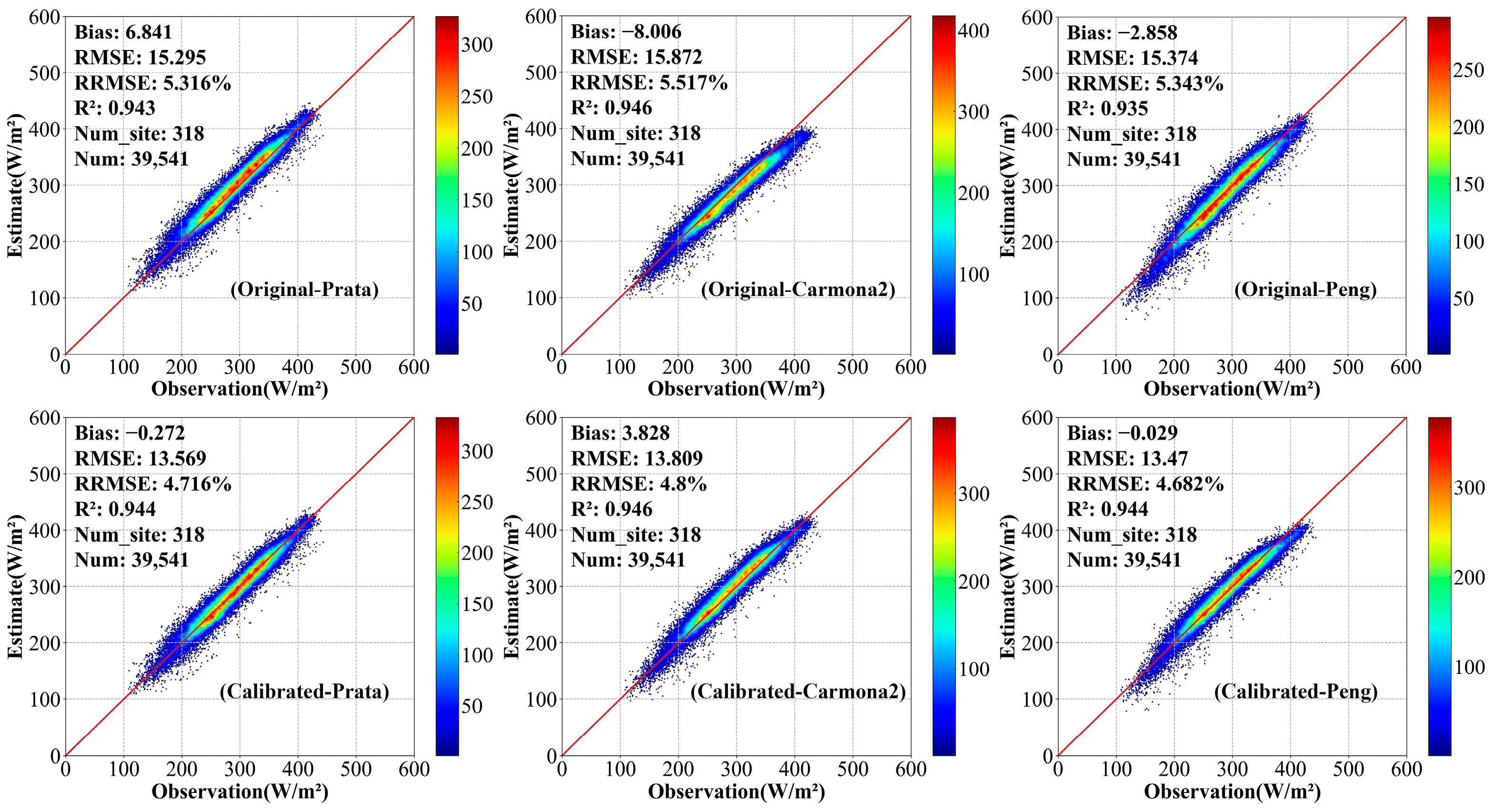
At a daily scale, with the calibrated coefficients of the three models for clear days (Table 6), their validation accuracies were very similar, but all improved by approximately 2 W / m 2 in RMSE after calibration (Figure 2). The models performed much better on the daily scale than on the hourly scale, a result consistent with the findings of Kjaersgaard et al. [23]. Particularly, the Peng model performed the best, yielding an RMSE of 13.47 W / m 2 , a bias of −0.029 W / m 2 , and an R2 of 0.944. Moreover, the Carmona2 model showed a tendency for overestimation (bias = 3.828 W / m 2 ).
Therefore, the Prata, Carmono2, and Peng models worked well with minor differences under clear-sky conditions at both hourly and daily scales, with the Peng model performing more robustly.

4.1.2. Cloudy-Sky

Under cloudy-sky conditions, the Carmona2, K-C, and Peng models were evaluated for cases4–6, respectively. Similarly, the calibrated coefficients for each model at an hourly scale are presented in Table 7. Additionally, Table 8 provides the validation accuracy of each model before and after calibration using the same validation samples.
In general, the accuracy of each model improved significantly after calibration, particularly for the Carmona2 model, which saw reductions in RMSEs of 14.039 W / m 2 (daytime) and 8.644 W / m 2 (nighttime) and biases of 23.392 W/m2 (daytime) and 13.123 W/m2 (nighttime). The daytime accuracies of all three models slightly surpassed those at nighttime, with each model experiencing a decline in RMSE values ranging from 1.127 to 2.303 W / m 2 , consistent with findings under clear-sky conditions. However, the SDLR models under cloudy-sky conditions at hourly scale performed worse than under clear-sky conditions (Table 5), indicating that clouds are one of the primary factors contributing to increased uncertainty in SDLR estimation [59,60]. Among the models, the Peng model demonstrated the most robust performer, consistently demonstrating superior accuracy under both daytime and nighttime conditions, both before and after calibration. After calibration, the Peng model exhibited RMSEs of 20.142 W / m 2 (daytime) and 21.308 W / m 2 (nighttime), biases of −0.027 W / m 2 (daytime) and 0.015 W / m 2 (nighttime), and R 2 values of 0.867 (daytime) and 0.864 (nighttime). The calibrated Carmona2 model followed.
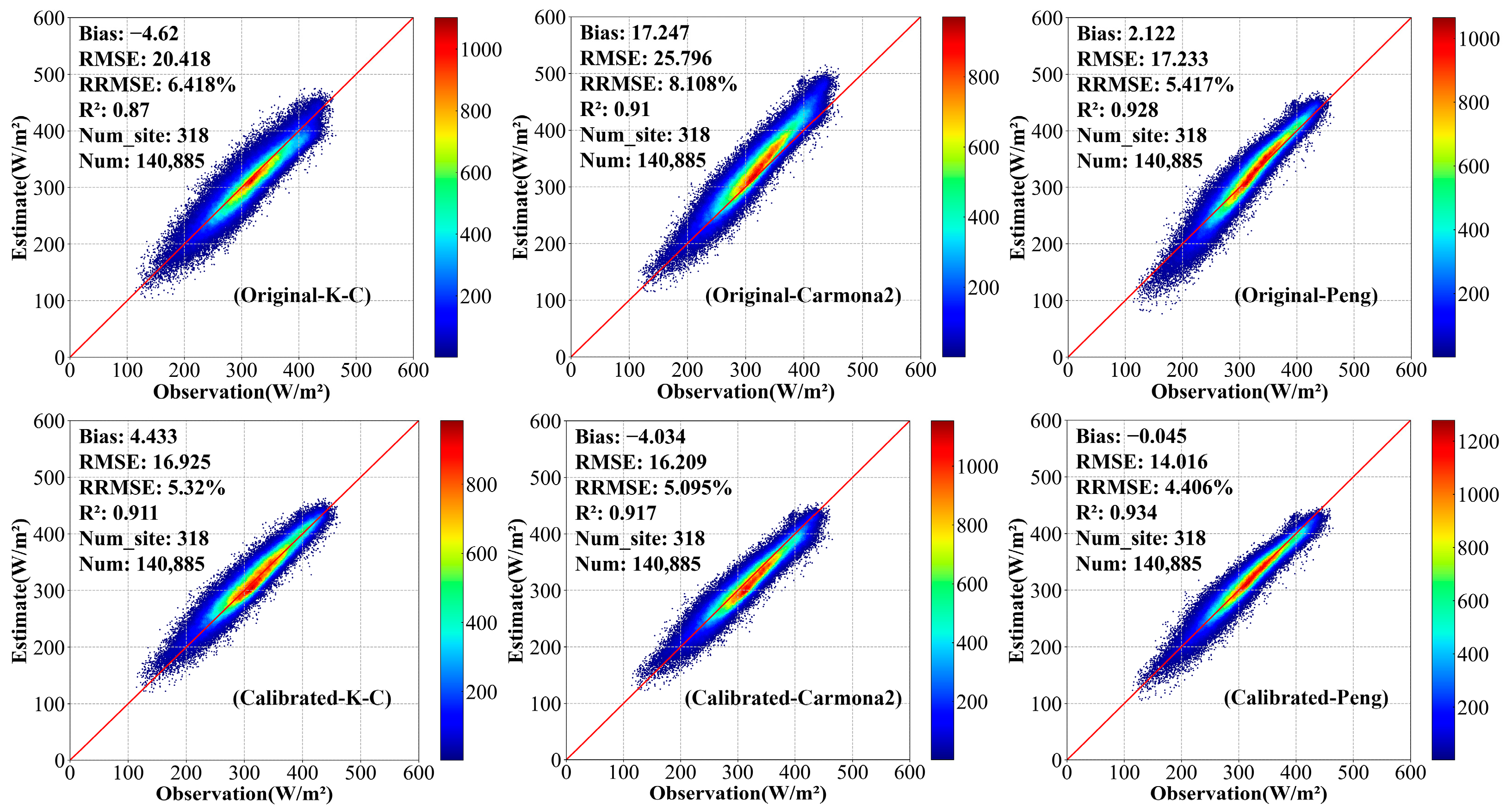
At the daily scale, as illustrated in Figure 3, the validation results were similar to those at the hourly scale. Using the calibration coefficients (Table 9), all three models demonstrated a remarkable improvement in estimation accuracy, with the Carmona2 model showing the most significant decrease in validated RMSE of 9.587 W / m 2 of the. Overall, the validation accuracies of all three models on a daily scale outperformed those on an hourly scale, with RMSE values ranging from 14.016 to 16.209 W / m 2 after calibration. Among the three models, the calibrated Peng model exhibited the highest accuracy, with its RMSE value lower than those of the other models by 2~3 W / m 2 and an R 2 of up to 0.934. Conversely, the K-C model performed the worst and tended to overestimate, while the Carmona2 model showed a tendency to underestimate.
In summary, it is suggested to calibrate all SDLR parameterization models with global training data before application. Although these four models performed worse under cloudy-sky conditions and at nighttime hours, the Peng model still demonstrated the most robust and best performance in all cases.

4.2. Model Performance under Various Conditions

For further exploration, the validation accuracies of the four calibrated SDLR models at a daily scale were further examined under various conditions, including land cover, elevation, and season. As previously discussed, the Carmona2 and Peng models were evaluated under both clear- and cloudy-sky conditions, whereas the Prata and K-C models were only evaluated under clear-sky and cloudy-sky conditions, respectively.
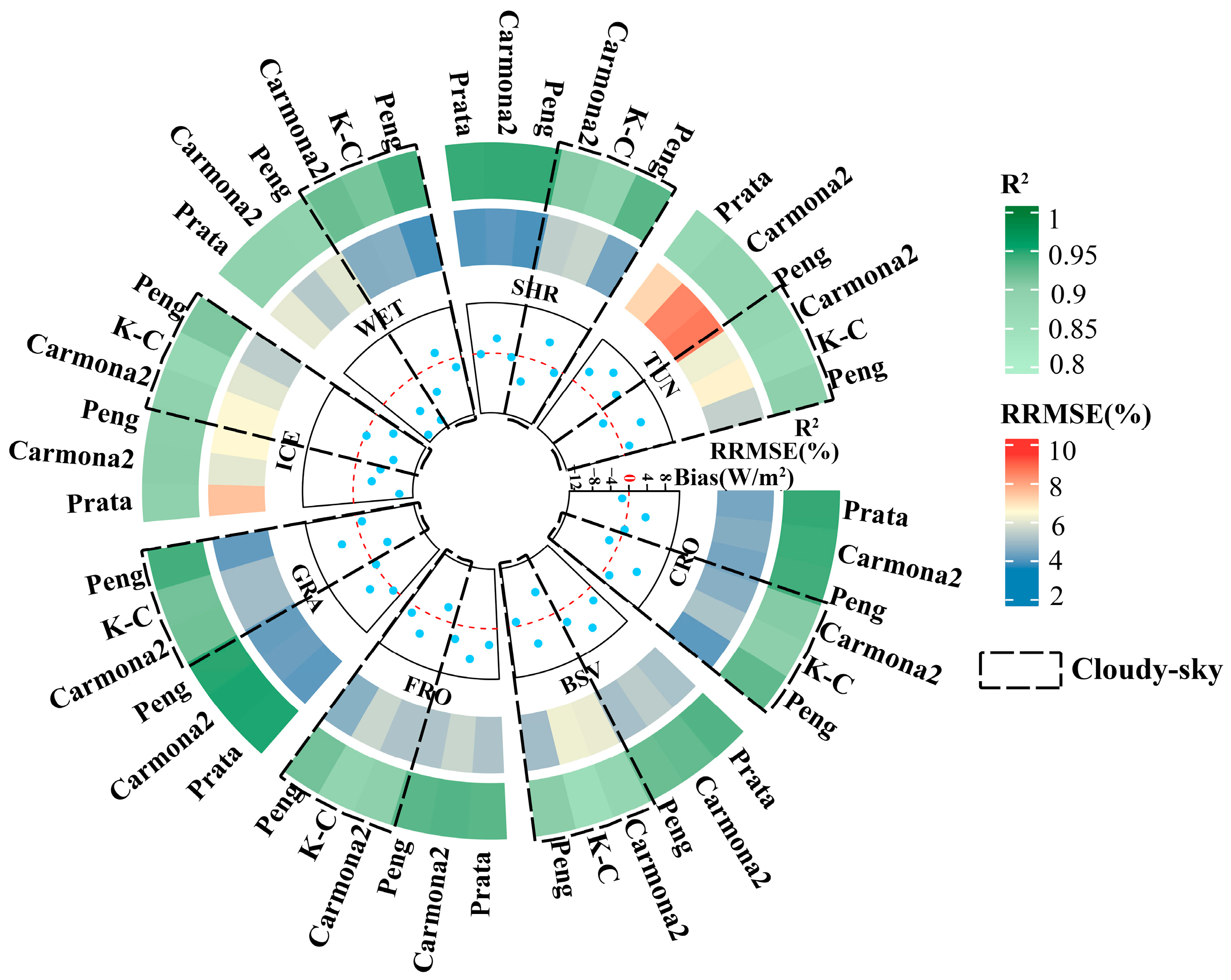
The evaluation results for the four models across eight land cover types are presented in Figure 4. Generally, these models performed better under clear-sky conditions than under cloudy-sky conditions (results in dashed boxes), except TUN, ICE with high albedo, and WET with seasonal variations. All models performed worse for these three land cover types, indicating that essential information on SDLR for these three land cover types has not been thoroughly explored, which aligns with the conclusions of Guo et al. [25]. Among the other five land cover types, all models performed the best for GRA and SHR. The Carmona2 model, in particular, exhibited the strongest tendency for overestimation or underestimation in SDLR, with the largest bias magnitude for most land cover types. However, for ICE and WET, the Carmono2 model worked the best under clear-sky conditions. Surprisingly, the Prata model worked the best for TUN. The Peng model showed significant superiority with the smallest RRMSE and bias for nearly all land cover types under all-sky conditions, suggesting it is suitable for daily SDLR estimation, especially on cloudy days.
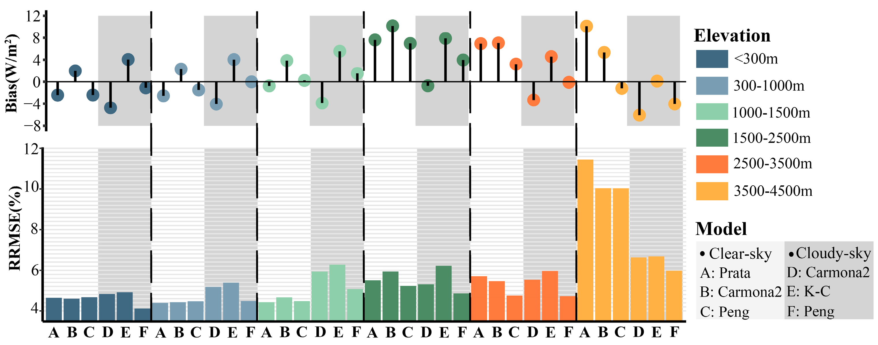
Figure 5 illustrates the estimation accuracies of the four SDLR models across different elevation zones. Six elevation zones (<300 m, 300–1000 m, 1000–1500 m, 1500–2500 m, 2500–3500 m, 3500–4500 m) were considered. Overall, the daily SDLR estimation accuracy of these models was better for clear days than for cloudy days, with generally smaller RRMSE and bias magnitude only, except for the elevation zone above 3500 m. All the model estimation accuracies increased with elevation, yielding RRMSE ranging from 10.03% to 11.45% under clear-sky conditions and from 5.98% to 6.68% under cloudy-sky conditions, respectively. Consistent with the results for different land cover types, the Peng model still performed robustly and better under all-sky conditions across all elevation zones, especially under cloudy-sky conditions.
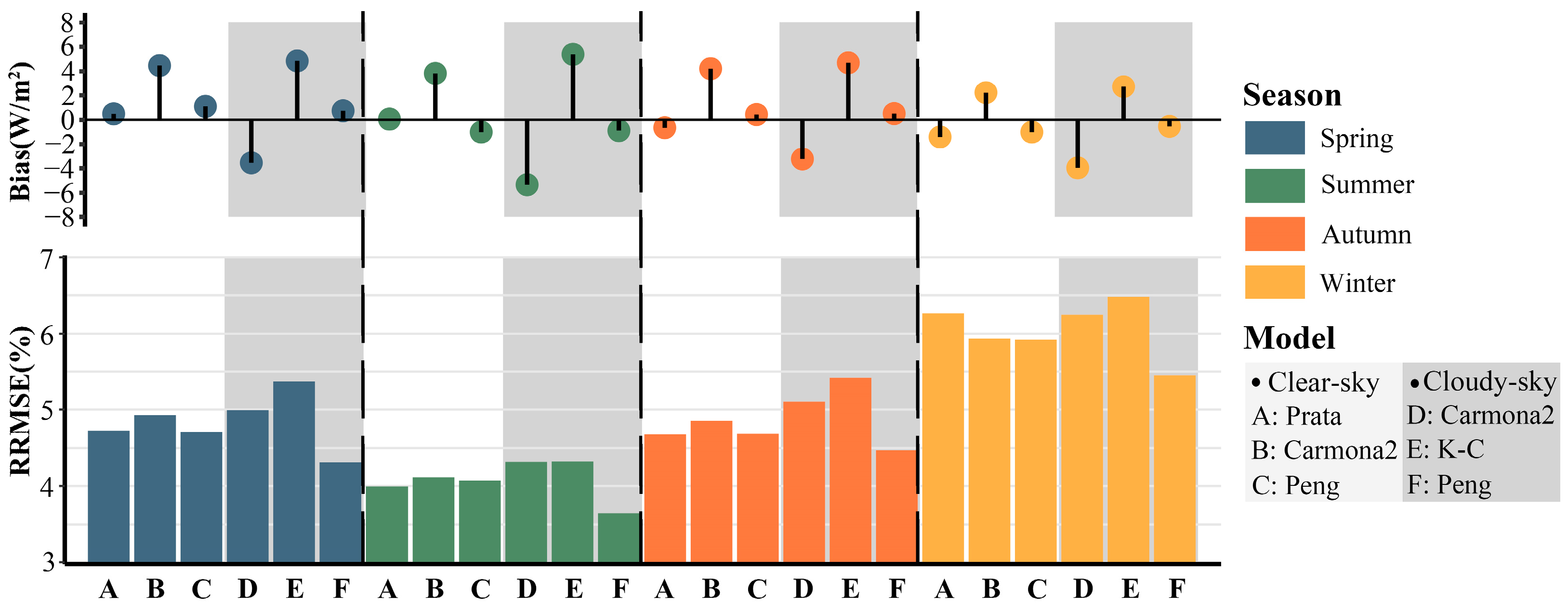
Moreover, the performance of the four models across four seasons is displayed in Figure 6. The four seasons were divided into Spring (Mar.–May), Summer (Jun.–Aug.), Autumn (Sep.–Nov.), and Winter (Dec.–Feb.). It is evident that all models performed worst in winter (RRMSE ranging from 5.45% to 6.48%) and best in summer (RRMSE ranging from 3.65% to 4.32%), with moderate performance in spring and autumn. The Prata and Peng models showed slight superiority over the Carmona2 model under clear-sky conditions (except in winter). Additionally, the Peng model exhibited a notable advantage under cloudy-sky conditions, reducing RRMSE by 0.63% to 1.06% compared to that of the Carmona2 and K-C models. Consistent with previous conclusions, the Carmona2 model tended to overestimate under clear-sky conditions and underestimate under cloudy-sky conditions across all seasons, whereas the K-C model consistently exhibited a tendency to overestimate.
In a word, the Peng model is one of the most optimal models for daily SDLR estimation compared to the other three models. However, all SDLR models require improvements for specific land cover types (i.e., ICE, WET, and TUN) and high-elevation zones.

4.3. Inter-Comparison with Three Existing SDLR Products

4.3.1. Comparison Results

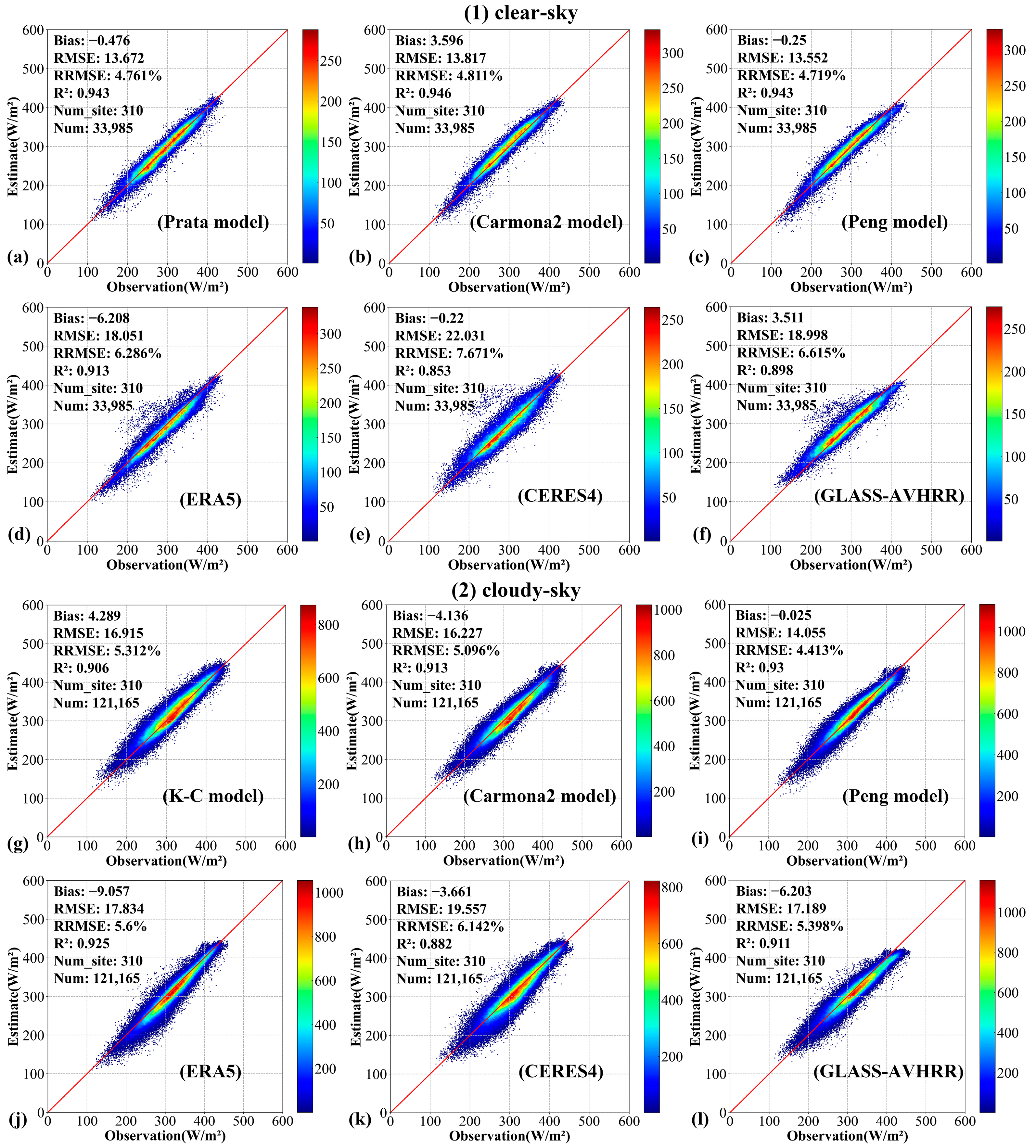
Subsequently, the accuracy of the four SDLR parameterization models was compared with three existing SDLR products, ERA5, CERES4, and GLASS-AVHRR, by validating against common independent validation samples at both hourly and daily scales under clear- and cloudy-sky conditions, respectively. Note that GLASS-AVHRR only provides daily SDLR products. Table 10 and Figure 7 present the overall validation results of all SDLR models and products at hourly and daily scales, respectively.
Consistent with previous findings, Table 10 shows that the Peng model worked the best under all-sky at hourly, with the smallest RMSE of 17.327 and 20.748 W/m2 and Bias magnitude of −0.074 and −0.046 W/m2 for clear- and cloudy-sky, respectively. In comparison, the accuracy of all model estimates was better than that of the two products. Relatively, ERA5 hourly SDLR tended to be severely underestimated under all sky conditions (Bias of −7.420 under a clear sky and −9.701 W / m 2 under the cloudy sky), though its RMSE was smaller than that of CERES4. Overall, all estimates performed relatively better without clouds.
At daily scale, for clear days (Figure 7a–f), the accuracy of the estimates from three models (Prata, Carmona2, and Peng model) were similar, with their RMSE ranging from 13.552~13.817 W / m 2 , only with the overestimation observed for the Carmona2 model (Bias = 3.596 W / m 2 ). The three model results were all much better than those of the three products, and the accuracy of ERA5 and GLASS-AVHRR was close, but the underestimation was also the largest for ERA5 (Bias = −6.208 W / m 2 ). Similarly, for cloudy days (Figure 7g–l), the Peng model also showed superior performance with the smallest RMSE (14.055 W / m 2 ) and Bias (−0.025 W / m 2 ), and all products performed worse than all models and tended to be underestimated, especially ERA5 with the largest Bias magnitude (−9.057 W / m 2 ). Notably, the bias magnitude increased for nearly all estimates except for the Peng model, further highlighting the Peng model’s robust performance under cloudy-sky conditions.
In summary, the Peng model demonstrated significant advantages over the other three models and three SDLR products. Among the three products, GLASS-AVHRR and ERA5 ranked second with similar performance. However, their uncertainties were larger for ice-covered high latitudes and during winter days. Subsequently, further analysis of the Peng model is given below.

4.3.2. Further Analysis of the Peng Model

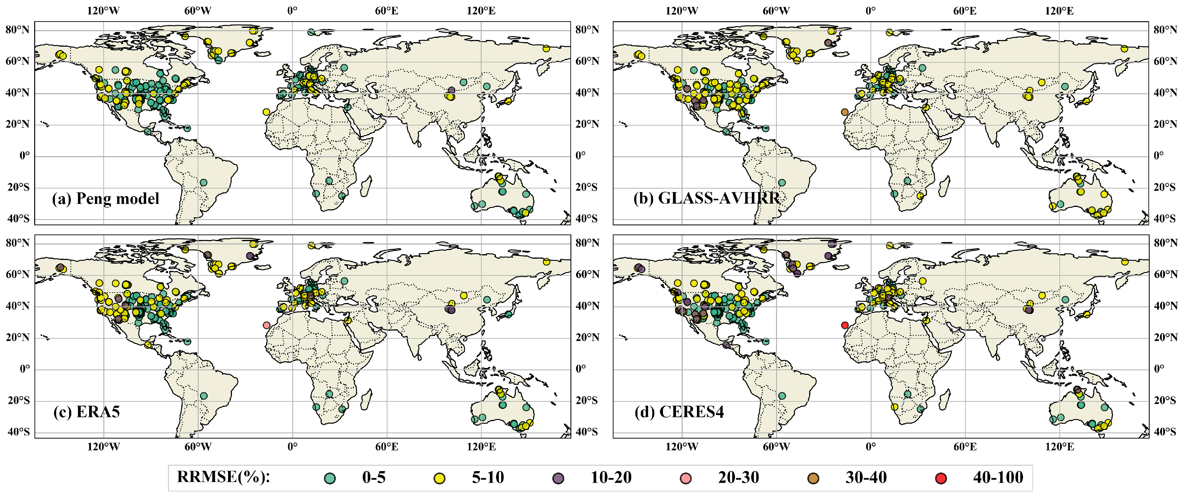
In order to examine the performance of the Peng model globally, the spatial distribution of the site validation accuracy daily is shown in Figure 8, and the same results of the three products are also given for comparison. It is seen that the Peng model demonstrated the most robustness globally, though all estimates performed poorly in the Polar Regions. Moreover, the accuracy of daily SDLR estimates was generally worse in western North America compared to eastern North America.
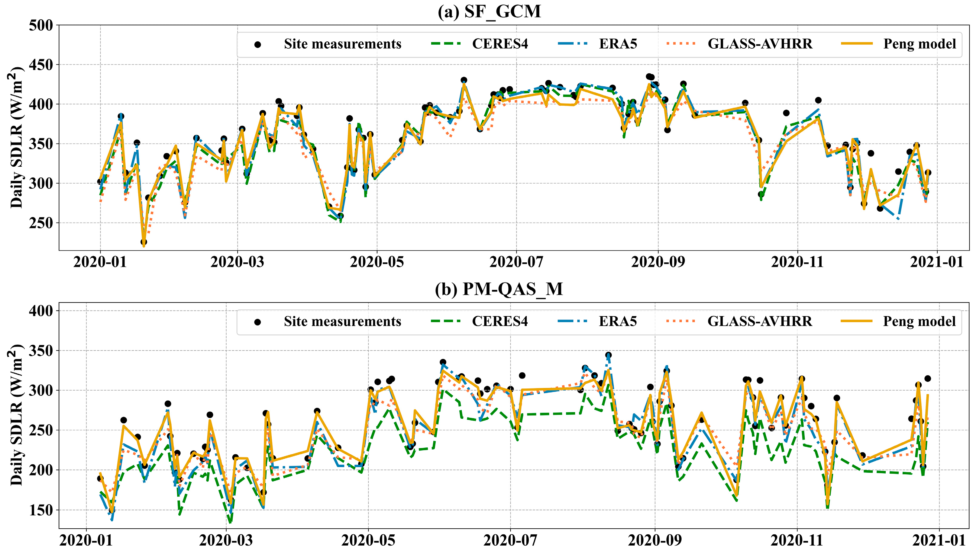
Meanwhile, the time series of the four daily SDLR estimates at two randomly selected stations (SF_GCM: 34.25°N, 89.87°W, Grassland; PM-QAS_L: 61.100°N, −46.833°W, ICE) were examined to assess their long-term variations, as shown in Figure 9. The in situ measurements (black dots) were added to each plot as a reference. Generally, the estimates from the Peng model and the three products were able to roughly capture the variations in SDLR at the two sites, but they all tended to underestimate SDLR, particularly in winter and for ICE. Comparatively, the estimates from the Peng model and GLASS-AVHRR were close to each other, but the ones from the Peng model were closer to the in situ measurements. The underestimation was most severe for CERES4 at the ICE site.
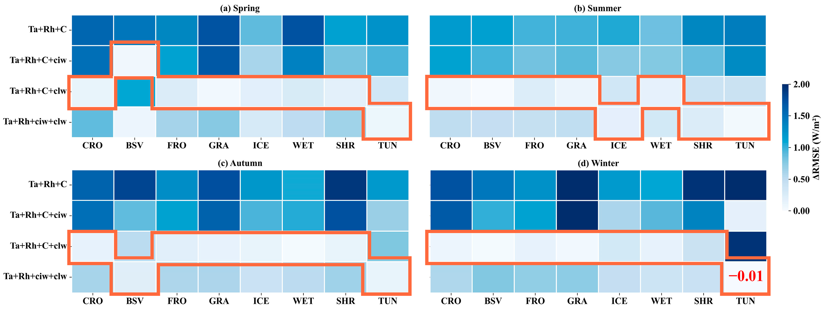
From all the above results, the significant advantages of the Peng model over the other three models and three SDLR products, particularly under a cloudy sky, are most possibly because of the two cloud-related parameters clw and ciw included besides the three commonly used parameters, Ta, RH, and C. However, the Peng model was initially proposed for sea surface; hence, the effectiveness of these variables for land surface application in the Peng model is analyzed. Against the same validation samples, the validated RMSE values of the Peng model with different combinations of the five input variables were calculated separately for various cases. Then, the differences in ΔRMSE, obtained by subtracting the RMSE of the original Peng model (Equation (12)) in the corresponding scenarios, are presented in Figure 10.
It is evident that introducing C, clw, and ciw into the Peng model yielded insignificant improvements (small ΔRMSE) under a clear sky. However, under cloudy-sky conditions, the ciw was less important than clw in the Peng model. For daily SDLR estimation, C + clw is suggested, whereas clw + ciw worked better for hourly scale, particularly during nighttime.
Combined with the results in Figure 11, for cloudy daily SDLR estimations across most land cover types across four seasons, the combination of C and clw yielded a similar performance to that of the original Peng model. The inclusion of ciw was only necessary for specific cases, such as for TUN across four seasons and BSV in autumn, which may be attributed to the typically lower temperatures and unique climatic conditions, facilitating the formation of high-altitude clouds where the impact of ciw on radiation becomes more pronounced. Besides TUN, the parameters clw and ciw were enough to provide cloud information for BSV, ICE, and SHR in some seasons, especially in summer. These results suggest that the insufficient information provided by C for cloudy skies can be effectively supplemented by ciw and clw, with the two cloud-related parameters playing different roles in various cases, thus requiring flexible selection, especially ciw, which is only extra needed when the high-altitude clouds appear (i.e., TUN).

5. Conclusions

The parameterization of SDLR models is widely utilized in practical applications due to their simplicity, efficiency, and acceptable accuracy. Given the abundance of SDLR parameterization models, especially newly developed ones, objective evaluation is crucial. Based on extensive ground measurements collected from 318 globally distributed stations, this study comprehensively evaluated three existing popular SDLR parameterization models, the Prata model, Carmona2 model, and the K-C model, alongside a newly proposed model, the Peng model. The evaluations considered clear-/cloudy-sky conditions at both hourly (daytime and nighttime) and daily scales.
The results demonstrated that the calibrated Peng model, which was applied for the first time to the land surface, outperformed the other models in terms of estimation accuracy and robustness across nearly all cases. Specifically, the discrepancies among the four models were minimal under clear-sky conditions. However, the advantage of the Peng model was significant under cloudy-sky conditions for both hourly (daytime and nighttime) and daily scales. Subsequently, comparing the estimates from the four models with three existing SDLR products (GLASS-AVHRR, CERES4, and ERA5), all models showed better accuracy than the products. ERA5 and GLASS-AVHRR had similar accuracy, but ERA5 was significantly underestimated. Further analysis illustrated the robustness of the Peng model under various conditions, including different land cover types, elevation zones, and seasons. The success of this model can be attributed to the inclusion of two cloud-related parameters, clw and ciw, which have a close physical correlation with CBT. The results also indicated that cloud information represented only by C, as used in most existing models, is insufficient for estimating SDLR under cloudy-sky conditions. We can flexibly select ciw and clw to supplement cloud information based on different situations. Specifically, ciw is only needed additionally when high-altitude clouds are present (e.g., TUN). Furthermore, the estimation accuracy of all SDLR models should be improved for wetlands, bare soil, ice-covered surfaces, and high-elevation regions.
In conclusion, the Peng model has strong potential to be widely used for SDLR estimation for both land and sea surfaces because of its high accuracy, robust performance, and simple implementation. However, this study primarily relies on data from mid-latitude regions, with relatively few data points from high-latitude areas, which may affect representativeness. Future research should incorporate more high-quality data from high-latitude regions, diverse climate types, and various surface covers to ensure thorough model validation and accuracy. Additionally, enhancing the accuracy of longwave downward radiation models for wetlands, bare soils, ice-covered surfaces, and high-elevation regions will be a crucial focus for future studies.

Author Contributions

Conceptualization, B.J.; data curation, Y.C. and J.P.; formal analysis, Y.C., X.Y., and Y.Z.; methodology, B.J. and Y.C.; writing—original draft preparation, Y.C.; writing—review and editing, Y.C. and B.J.; supervision, B.J. and J.P.; funding acquisition, B.J. All authors have read and agreed to the published version of the manuscript.

Funding

This research was funded by the National Natural Science Foundation of China, grant number 42090012.

Data Availability Statement

The websites of ARM, AsiaFlux, BSRN, Lathuile, AmeriFlux, EFDC, HiWATER, SURFRAD, and PROMICE networks are shown in Table 2. The GLASS-AVHRR, CERES4, and ERA5 are available at https://glass-product.bnu.edu.cn/ (accessed on 11 September 2024), https://ceres.larc.nasa.gov/ (accessed on 11 September 2024) and https://cds.climate.copernicus.eu/cdsapp#!/home (accessed on 11 September 2024), respectively.

Acknowledgments

The authors extend their heartfelt gratitude to ARM, AsiaFlux, BSRN, Lathuile, AmeriFlux, EFDC, HiWATER, SURFRAD, and PROMICE networks for providing essential radiative and meteorological data. We also thank the laboratories and researchers who contributed to the development and technical support of the GLASS-AVHRR, CERES, and ERA5 datasets. Additionally, we are grateful to the reviewers for their valuable suggestions.

Conflicts of Interest

The authors declare no conflicts of interest.

References

  1. Idso, S.B.; Jackson, R.D. Thermal Radiation from Atmosphere. J. Geophys. Res. 1969, 74, 5397–5403. [Google Scholar] [CrossRef]
  2. Peng, L.; Li, W.; Ye, J.; Cheng, D.; Li, Y.; Cao, L. A Review of Parameterization Methods for Downward Shortwave and Longwave Radiation on the Surface. Acta Sci. Nat. Univ. Pekin. 2015, 51, 772–782. [Google Scholar]
  3. Yu, S.; Xin, X.; Liu, Q. Comparison of Atmospheric Downward Longwave Radiation Parameterizations. Adv. Earth Sci. 2011, 26, 751–762. [Google Scholar]
  4. Duarte, H.F.; Dias, N.L.; Maggiotto, S.R. Assessing daytime downward longwave radiation estimates for clear and cloudy skies in Southern Brazil. Agric. For. Meteorol. 2006, 139, 171–181. [Google Scholar] [CrossRef]
  5. Roesch, A.; Wild, M.; Ohmura, A.; Dutton, E.G.; Long, C.N.; Zhang, T. Assessment of BSRN radiation records for the computation of monthly means. Atmos. Meas. Tech. Discuss. 2010, 3, 4423–4457. [Google Scholar] [CrossRef]
  6. Zhang, Y.C.; Rossow, W.; Lacis, A. Calculation of surface and top of atmosphere radiative fluxes from physical quantities based on ISCCP data sets: 1. Method and sensitivity to input data uncertainties. J. Geophys. Res. Atmos. 1995, 100, 1149–1165. [Google Scholar] [CrossRef]
  7. Cheng, J.; Liang, S.; Wang, W.; Guo, Y. An efficient hybrid method for estimating clear-sky surface downward longwave radiation from MODIS data. J. Geophys. Res. Atmos. 2017, 122, 2616–2630. [Google Scholar] [CrossRef]
  8. Yang, F.; Cheng, J. A framework for estimating cloudy sky surface downward longwave radiation from the derived active and passive cloud property parameters. Remote Sens. Environ. 2020, 248, 111972. [Google Scholar] [CrossRef]
  9. Wang, T.; Shi, J.; Yu, Y.; Husi, L.; Gao, B.; Zhou, W.; Ji, D.; Zhao, T.; Xiong, C.; Chen, L. Cloudy-sky land surface longwave downward radiation (LWDR) estimation by integrating MODIS and AIRS/AMSU measurements. Remote Sens. Environ. 2018, 205, 100–111. [Google Scholar] [CrossRef]
  10. Zhou, W.; Shi, J.C.; Wang, T.X.; Peng, B.; Husi, L.; Yu, Y.C.; Zhao, R. New Methods for Deriving Clear-Sky Surface Longwave Downward Radiation Based on Remotely Sensed Data and Ground Measurements. Earth Space Sci. 2019, 6, 2071–2086. [Google Scholar] [CrossRef]
  11. Zhu, F.X.; Li, X.; Qin, J.; Yang, K.; Cuo, L.; Tang, W.J.; Shen, C.P. Integration of Multisource Data to Estimate Downward Longwave Radiation Based on Deep Neural Networks. IEEE Trans. Geosci. Remote Sens. 2022, 60, 4103015. [Google Scholar] [CrossRef]
  12. Xu, J.L.; Liang, S.L.; Ma, H.; He, T. Generating 5 km resolution 1981-2018 daily global land surface longwave radiation products from AVHRR shortwave and longwave observations using densely connected convolutional neural networks. Remote Sens. Environ. 2022, 280, 113223. [Google Scholar] [CrossRef]
  13. Ångström, A. A Study of the Radiation of the Atmosphere: Based upon Observations of the Nocturnal Radiation during Expeditions to Algeria and to California; Smithsonian Institution: Washington, DC, USA, 1915; Volume 65. [Google Scholar]
  14. Brunt, D. Notes on radiation in the atmosphere. Q. J. R. Meteorol. Soc. 1932, 58, 389–420. [Google Scholar] [CrossRef]
  15. Swinbank, W.C. Long-wave radiation from clear skies. Q. J. R. Meteorol. Soc. 1963, 89, 339–348. [Google Scholar] [CrossRef]
  16. Brutsaert, W. On a derivable formula for long-wave radiation from clear skies. Water Resour. Res. 1975, 11, 742–744. [Google Scholar] [CrossRef]
  17. Prata, A. A new long-wave formula for estimating downward clear-sky radiation at the surface. Q. J. R. Meteorol. Soc. 1996, 122, 1127–1151. [Google Scholar]
  18. Idso, S.B. A Set of Equations for Full Spectrum and 8-μm to 14-μm and 10.5-μm to 12.5-μm Thermal-Radiation from Cloudless Skies. Water Resour. Res. 1981, 17, 295–304. [Google Scholar] [CrossRef]
  19. Iziomon, M.G.; Mayer, H.; Matzarakis, A. Downward atmospheric longwave irradiance under clear and cloudy skies: Measurement and parameterization. J. Atmos. Sol.-Terr. Phys. 2003, 65, 1107–1116. [Google Scholar] [CrossRef]
  20. Lhomme, J.P.; Vacher, J.J.; Rocheteau, A. Estimating downward long-wave radiation on the Andean Altiplano. Agric. For. Meteorol. 2007, 145, 139–148. [Google Scholar] [CrossRef]
  21. Gupta, S.K.; Darnell, W.L.; Wilber, A.C. A parameterization for longwave surface radiation from satellite data: Recent improvements. J. Appl. Meteorol. Climatol. 1992, 31, 1361–1367. [Google Scholar] [CrossRef]
  22. Peng, J.; Jiang, B.; Liang, H.; Li, S.; Han, J.; Ingalls, T.C.; Cheng, J.; Yao, Y.; Jia, K.; Zhang, X. Development and Comparison of Empirical Models for All-sky Downward Longwave Radiation Estimation at the Ocean Surface Using Long-term Observations. Atmos. Meas. Tech. Discuss. 2024, 1–32. [Google Scholar] [CrossRef]
  23. Kjaersgaard, J.; Plauborg, F.; Hansen, S. Comparison of models for calculating daytime long-wave irradiance using long term data set. Agric. For. Meteorol. 2007, 143, 49–63. [Google Scholar] [CrossRef]
  24. Santos, C.A.C.d.; Silva, B.B.d.; Rao, T.V.R.; Satyamurty, P.; Manzi, A.O. Downward longwave radiation estimates for clear-sky conditions over northeast Brazil. Rev. Bras. Meteorol. 2011, 26, 443–450. [Google Scholar] [CrossRef]
  25. Guo, Y.; Cheng, J.; Liang, S. Comprehensive assessment of parameterization methods for estimating clear-sky surface downward longwave radiation. Theor. Appl. Climatol. 2019, 135, 1045–1058. [Google Scholar] [CrossRef]
  26. Cheng, J.; Yang, F.; Guo, Y. A comparative study of bulk parameterization schemes for estimating cloudy-sky surface downward longwave radiation. Remote Sens. 2019, 11, 528. [Google Scholar] [CrossRef]
  27. Carmona, F.; Rivas, R.; Caselles, V. Estimation of daytime downward longwave radiation under clear and cloudy skies conditions over a sub-humid region. Theor. Appl. Climatol. 2014, 115, 281–295. [Google Scholar] [CrossRef]
  28. Phillips, T.J.; Klein, S.A.; Ma, H.Y.; Tang, Q.; Xie, S.C.; Williams, I.N.; Santanello, J.A.; Cook, D.R.; Torn, M.S. Using ARM Observations to Evaluate Climate Model Simulations of Land-Atmosphere Coupling on the US Southern Great Plains. J. Geophys. Res.-Atmos. 2017, 122, 11524–11548. [Google Scholar] [CrossRef]
  29. Yu, G.R.; Hirano, T. Review and future perspective of AsiaFlux. J. Agric. Meteorol. 2021, 77, 1. [Google Scholar] [CrossRef]
  30. Driemel, A.; Augustine, J.; Behrens, K.; Colle, S.; Cox, C.; Cuevas-Agulló, E.; Denn, F.M.; Duprat, T.; Fukuda, M.; Grobe, H. Baseline Surface Radiation Network (BSRN): Structure and data description (1992–2017). Earth Syst. Sci. Data 2018, 10, 1491–1501. [Google Scholar] [CrossRef]
  31. Yi, C.; Ricciuto, D.; Li, R.; Wolbeck, J.; Xu, X.; Nilsson, M.; Aires, L.; Albertson, J.D.; Ammann, C.; Arain, M.A. Climate control of terrestrial carbon exchange across biomes and continents. Environ. Res. Lett. 2010, 5, 034007. [Google Scholar] [CrossRef]
  32. Novick, K.A.; Biederman, J.; Desai, A.; Litvak, M.; Moore, D.J.; Scott, R.; Torn, M. The AmeriFlux network: A coalition of the willing. Agric. For. Meteorol. 2018, 249, 444–456. [Google Scholar] [CrossRef]
  33. Li, X.; Liu, S.; Ma, M.; Xiao, Q.; Liu, Q.; Jin, R.; Che, T.; Wang, W.; Qi, Y.; Li, H.; et al. HiWATER:An Integrated Remote Sensing Experiment on Hydrological and Ecological Processes in the Heihe River Basin. Adv. Earth Sci. 2012, 27, 481–498. [Google Scholar]
  34. Augustine, J.A.; Hodges, G.B.; Cornwall, C.R.; Michalsky, J.J.; Medina, C.I. An update on SURFRAD—The GCOS surface radiation budget network for the continental United States. J. Atmos. Ocean. Technol. 2005, 22, 1460–1472. [Google Scholar] [CrossRef]
  35. Fausto, R.S.; van As, D.; Mankoff, K.D.; Vandecrux, B.; Citterio, M.; Ahlstrom, A.P.; Andersen, S.B.; Colgan, W.; Karlsson, N.B.; Kjeldsen, K.K.; et al. Programme for Monitoring of the Greenland Ice Sheet (PROMICE) automatic weather station data. Earth Syst. Sci. Data 2021, 13, 3819–3845. [Google Scholar] [CrossRef]
  36. Wang, K.; Liang, S. Estimation of daytime net radiation from shortwave radiation measurements and meteorological observations. J. Appl. Meteorol. Climatol. 2009, 48, 634–643. [Google Scholar] [CrossRef]
  37. Li, S.; Jiang, B.; Peng, J.; Liang, H.; Han, J.; Yao, Y.; Zhang, X.; Cheng, J.; Zhao, X.; Liu, Q. Estimation of the all-wave all-sky land surface daily net radiation at mid-low latitudes from MODIS data based on ERA5 constraints. Remote Sens. 2021, 14, 33. [Google Scholar] [CrossRef]
  38. Liu, B.Y.; Jordan, R.C. The interrelationship and characteristic distribution of direct, diffuse and total solar radiation. Sol. Energy 1960, 4, 1–19. [Google Scholar] [CrossRef]
  39. Yin, X.; Jiang, B.; Liang, S.; Li, S.; Zhao, X.; Wang, Q.; Xu, J.; Han, J.; Liang, H.; Zhang, X. Significant discrepancies of land surface daily net radiation among ten remotely sensed and reanalysis products. Int. J. Digit. Earth 2023, 16, 3725–3752. [Google Scholar] [CrossRef]
  40. Mousavi Maleki, S.A.; Hizam, H.; Gomes, C. Estimation of hourly, daily and monthly global solar radiation on inclined surfaces: Models re-visited. Energies 2017, 10, 134. [Google Scholar] [CrossRef]
  41. Flerchinger, G.; Xaio, W.; Marks, D.; Sauer, T.; Yu, Q. Comparison of algorithms for incoming atmospheric long-wave radiation. Water Resour. Res. 2009, 45. [Google Scholar] [CrossRef]
  42. Irmak, S.; Irmak, A.; Jones, J.W.; Howell, T.; Jacobs, J.M.; Allen, R.G.; Hoogenboom, G. Predicting daily net radiation using minimum climatological data. J. Irrig. Drain. Eng. 2003, 129, 256–269. [Google Scholar] [CrossRef]
  43. Hersbach, H.; Bell, B.; Berrisford, P.; Hirahara, S.; Horányi, A.; Muñoz-Sabater, J.; Nicolas, J.; Peubey, C.; Radu, R.; Schepers, D. The ERA5 global reanalysis. Q. J. R. Meteorol. Soc. 2020, 146, 1999–2049. [Google Scholar] [CrossRef]
  44. Simmons, A. ERA-Interim: New ECMWF reanalysis product from 1989 onwards. Ecmwf Newsl. 2006, 110, 25. [Google Scholar]
  45. Yao, B.; Teng, S.; Lai, R.; Xu, X.; Yin, Y.; Shi, C.; Liu, C. Can atmospheric reanalyses (CRA and ERA5) represent cloud spatiotemporal characteristics? Atmos. Res. 2020, 244, 105091. [Google Scholar] [CrossRef]
  46. Tang, W.; Qin, J.; Yang, K.; Zhu, F.; Zhou, X. Does ERA5 outperform satellite products in estimating atmospheric downward longwave radiation at the surface? Atmos. Res. 2021, 252, 105453. [Google Scholar] [CrossRef]
  47. Wielicki, B.A.; Barkstrom, B.R.; Harrison, E.F.; Lee III, R.B.; Smith, G.L.; Cooper, J.E. Clouds and the Earth’s Radiant Energy System (CERES): An earth observing system experiment. Bull. Am. Meteorol. Soc. 1996, 77, 853–868. [Google Scholar] [CrossRef]
  48. Fu, Q.; Liou, K.N. Parameterization of the Radiative Properties of Cirrus Clouds. J. Atmos. Sci. 1993, 50, 2008–2025. [Google Scholar] [CrossRef]
  49. Fu, Q.; Lesins, G.; Higgins, J.; Charlock, T.; Chylek, P.; Michalsky, J. Broadband water vapor absorption of solar radiation tested using ARM data. Geophys. Res. Lett. 1998, 25, 1169–1172. [Google Scholar] [CrossRef]
  50. Rutan, D.A.; Kato, S.; Doelling, D.R.; Rose, F.G.; Caldwell, T.E.; Loeb, N.G. CERES synoptic product: Methodology and validation of surface radiant flux. J. Atmos. Ocean. Technol. 2015, 32, 1121–1143. [Google Scholar] [CrossRef]
  51. Xu, J.L.; Liang, S.L.; He, T.; Ma, H.; Zhang, Y.F.; Zhang, G.D.; Liang, H. Variability and trends in land surface longwave radiation fluxes from six satellite and reanalysis products. Int. J. Digit. Earth 2023, 16, 2912–2940. [Google Scholar] [CrossRef]
  52. Konzelmann, T.; van de Wal, R.S.; Greuell, W.; Bintanja, R.; Henneken, E.A.; Abe-Ouchi, A. Parameterization of global and longwave incoming radiation for the Greenland Ice Sheet. Glob. Planet. Chang. 1994, 9, 143–164. [Google Scholar] [CrossRef]
  53. Robinson, G. Notes on the measurement and estimation of atmospheric radiation. Q. J. R. Meteorol. Soc. 1947, 73, 127–150. [Google Scholar] [CrossRef]
  54. Robinson, G. Notes on the measurement and estimation of atmospheric radiation–2. Q. J. R. Meteorol. Soc. 1950, 76, 37–51. [Google Scholar] [CrossRef]
  55. Carmona, F.; Rivas, R.; Ocampo, D.; Schirmbeck, J.; Holzman, M. Sensores para la medición y validación de variables Hidrológicas a escalas local y regional a partir del balance de energía. Aqua-LAC 2011, 3, 26–36. [Google Scholar] [CrossRef]
  56. Bignami, F.; Marullo, S.; Santoleri, R.; Schiano, M. Longwave radiation budget in the Mediterranean Sea. J. Geophys. Res. Ocean. 1995, 100, 2501–2514. [Google Scholar] [CrossRef]
  57. Clark, N.; Eber, L.E.; Laurs, R.M.; Renneer, J.; Saur, J. Heat exchange between ocean and atmosphere in the eastern North Pacific for 1961–71. 1974. Available online: https://repository.library.noaa.gov/view/noaa/11864/ (accessed on 28 July 2024).
  58. Frouin, R.; Gautier, C.; Morcrette, J.J. Downward longwave irradiance at the ocean surface from satellite data: Methodology and in situ validation. J. Geophys. Res. Ocean. 1988, 93, 597–619. [Google Scholar] [CrossRef]
  59. Trenberth, K.E.; Fasullo, J.T.; Kiehl, J. Earth’s global energy budget. Bull. Am. Meteorol. Soc. 2009, 90, 311–324. [Google Scholar] [CrossRef]
  60. Wild, M.; Ohmura, A.; Gilgen, H.; Morcrette, J.-J.; Slingo, A. Evaluation of downward longwave radiation in general circulation models. J. Clim. 2001, 14, 3227–3239. [Google Scholar] [CrossRef]
Figure 1. Spatial distribution of the 318 sites in nine surface radiation observing networks. Detailed information about the nine observing networks is provided in Table 2.
Remotesensing 16 03422 g001
Figure 2. Validation accuracy of the Prata, Carmona2, and Peng models with the original and calibrated coefficients at daily scales under clear-sky conditions. The color bar indicates the number of samples.
Remotesensing 16 03422 g002
Figure 3. The same as Figure 2, but for the K-C, Carmona2, and Peng models under cloudy-sky conditions.
Remotesensing 16 03422 g003
Figure 4. Validation accuracies of the four evaluated SDLR models at a daily scale for eight land cover types under clear- and cloudy-sky conditions. The dashed boxes indicate the results under a cloudy sky.
Remotesensing 16 03422 g004
Figure 5. The same as Figure 4, but for six elevation zones (<300 m, 300–1000 m, 1000–1500 m, 1500–2500 m, 2500–3500 m, 3500–4500 m). The results under cloudy-sky conditions are added to the gray background.
Remotesensing 16 03422 g005
Figure 6. The same as Figure 5, but for four seasons: Spring (Mar.–May), Summer (Jun.–Aug.), Autumn (Sep.–Nov.), and Winter (Dec.–Feb.).
Remotesensing 16 03422 g006
Figure 7. Overall validation accuracy of the four SDLR models and three products (ERA5, CERES4, and GLASS-AVHRR) at daily scales under clear- (af) and (gl) cloudy-sky conditions.
Remotesensing 16 03422 g007
Figure 8. The spatial distribution of the validated RRMSE at site scale for (a) Peng model and (bd) three products (GLASS-AVHRR, ERA5, CERES4).
Remotesensing 16 03422 g008
Figure 9. The time series of the daily SDLR from the Peng model and other three products at two sites (a) SF_GCM (34.25°N, 89.87°W, Grassland) and (b) PM-QAS_M (61.100°N, −46.833°W, ICE).
Remotesensing 16 03422 g009
Figure 10. Differences in the validated RMSE (ΔRMSE) between the Peng models with different combinations of the five input variables and the original one (all five variables).
Remotesensing 16 03422 g010
Figure 11. The same as Figure 10, but on a daily scale under cloudy-sky conditions for the four seasons. The red box indicates the smallest ΔRMSE. Note that a negative ΔRMSE indicates that the corresponding combination of variables in the Peng model performed better than the original one.
Remotesensing 16 03422 g011
Table 1. All variables used in this study and their sources.
Abbr.Full NameTime ScalesUnitData Source
DSRDownward shortwave radiationDaily/hourlyW/m2In situ
USRUpward shortwave radiationDaily/hourlyW/m2
SDLRSurface downward longwave radiationDaily/hourlyW/m2
TaAir temperature at 2 m above the surfaceDaily/hourlyK
RHRelative humidityDaily/hourly%
SnShortwave net radiationDaily/hourlyW/m2Calculated
eaWater vapor pressureDaily/hourlyhPa
CIClearness IndexDaily/hourly\
CCloud fraction (total cloud volume)Daily/hourly0–1ERA5
clwTotal column cloud liquid waterDaily/hourlyg/m3
ciwTotal column cloud ice waterDaily/hourlyg/m3
Table 2. Details of the nine observation networks.
NetworkFull NameNo. of SitesTime PeriodSampling Frequency
/min
URLReference
ARMThe Atmospheric Radiation Measurement331994–20191https://www.archive.arm.gov, accessed on 11 September 2024.[28]
AsiaFluxAsia Flux dataset142001–201430https://db.cger.nies.go.jp/asiafluxdb/?page_id=16, accessed on 11 September 2024.[29]
BSRNthe Baseline Surface Radiation Network441992–20211/3https://bsrn.awi.de, accessed on 11 September 2024.[30]
LathuileGlobal Fluxnet651996–201430https://fluxnet.fluxdata.org, accessed on 11 September 2024.[31]
AmeriFluxAmeriFlux1781996–202130https://ameriflux.lbl.gov, accessed on 11 September 2024.[32]
EFDCThe European Eddy Fluxes Database Cluster601997–202130http://www.europe-fluxdata.eu/, accessed on 11 September 2024.
HiWATERHeihe Watershed Allied Telemetry Experimental Research182012–202010http://data.tpdc.ac.cn/zh-hans/, accessed on 11 September 2024.[33]
SURFRADthe Surface Radiation Budget Observing Network71995–20213ftp://aftp.cmdl.noaa.gov/data/radiation/surfrad/, accessed on 11 September 2024.[34]
PROMICEPROMICE222007–202160https://www.promice.org, accessed on 11 September 2024.[35]
Table 3. Details of the samples used for model training and validation for each case.
Case ExplanationTraining SamplesValidation Samples
Case1Clear-skyHourlyDaytime1,067,240457,400
Case2Nighttime654,175280,389
Case3Daily\92,20439,541
Case4Cloudy-skyHourlyDaytime2,853,0721,222,767
Case5Nighttime2,643,8851,133,106
Case6Daily\328,701140,885
Table 4. The calibrated coefficients of the Prata, Carmona2, and Peng models under clear-sky conditions at an hourly scale.
Model abdefg
PrataDaytime0.9722.780
Nighttime1.1302.989
Carmona2Daytime−0.648 4.4 × 10 3 2.1 × 10 3
Nighttime−0.378 3.6 × 10 3 1.8 × 10 3
PengDaytime1.0268.5522.5620.7380.806−156.605
Nighttime0.9808.5511.6605.0960.661−124.783
Table 5. Validation accuracy of the Prata, Carmona2, and Peng models with their original and calibrated coefficients at hourly scale under clear-sky conditions.
SituationDaytimeNighttime
PrataCarmona2PengPrataCarmona2Peng
OriginalBias (W/m2)11.972−5.486−0.9381.488−9.068−8.764
RMSE (W/m2)20.60118.28717.73418.76120.20121.218
RRMSE (%)6.8216.0555.8726.8957.4247.797
R20.9350.9340.9290.8960.9040.897
CalibrationBias (W/m2)0.008−4.7490.026−0.368−1.2630.005
RMSE (W/m2)16.67917.31616.91718.66417.85917.793
RRMSE (%)5.5235.7335.6016.8596.5636.539
R20.9350.9350.9330.8970.9050.905
Table 6. The calibration coefficients of the Prata, Carmona2, and Peng models under clear-sky conditions at a daily scale.
Modelabdefg
Prata1.0582.852
Carmona2−0.521 4   ×   10 3 2   ×   10 3
Peng1.0115.5561.0461.3210.773−145.236
Table 7. The same as Table 4 but for the K-C, Carmona2, and Peng models under cloudy-sky conditions.
ModelTimeabdefg
K-CDaytime0.275 1.5 × 10 3 2.5 × 10 3 453.2940.915
Nighttime0.302 1.3 × 10 3 2.3 × 10 3 78.1880.929
Carmona2Daytime0.316 1.2 × 10 3 2.4 × 10 3 0.068
Nighttime0.379 0.8 × 10 3 2.3 × 10 3 0.113
PengDaytime0.88814.3144.9052.5580.761−94.553
Nighttime0.871115.5775.1643.9250.611−84.064
Table 8. The same as Table 5, but for the K-C, Carmona2, and Peng models under cloudy-sky conditions.
SituationDaytimeNighttime
Carmona2K-CPengCarmona2K-CPeng
OriginalBias (W/m2)23.5952.2032.19818.2580.720.014
RMSE (W/m2)36.24232.0223.12333.1529.43125.102
RRMSE (%)10.8039.5446.89210.8039.5918.181
R20.8090.6960.8550.8190.7520.846
CalibrationBias (W/m2)0.521−1.289−0.0275.1351.9260.015
RMSE (W/m2)22.20323.77420.14224.50624.90221.308
RRMSE (%)6.6187.0866.0047.9868.1156.944
R20.8390.8160.8670.8280.8150.864
Table 9. The same as Table 6 but for the K-C, Carmona2, and Peng models under cloudy-sky conditions.
Modelabdefg
K-C0.070 2   ×   10 3 2.6 × 10 3 7.6620.938
Carmona20.218 1.4 × 10 3 2.3 × 10 3 0.118
Peng0.90529.9244.4591.8710.686−109.290
Table 10. Validation accuracy of the SDLR estimates from four models and two products (ERA5, CERES4) at an hourly scale.
IndicesModelClear-SkyCloudy-SkyProductClear-SkyCloudy-Sky
Bias (W/m2)Prata model−0.224 ERA5−7.420−9.701
RMSE (W/m2)17.53021.03525.851
R20.9260.9070.845
Bias (W/m2)K-C model 0.228CERES41.620−3.571
RMSE (W/m2)24.34925.62227.770
R20.8250.8490.802
Bias (W/m2)Carmona2 model−3.5092.706
RMSE (W/m2)17.61023.355
R20.9280.841
Bias (W/m2)Peng model−0.074−0.046
RMSE (W/m2)17.32720.748
R20.9270.873
Disclaimer/Publisher’s Note: The statements, opinions and data contained in all publications are solely those of the individual author(s) and contributor(s) and not of MDPI and/or the editor(s). MDPI and/or the editor(s) disclaim responsibility for any injury to people or property resulting from any ideas, methods, instructions or products referred to in the content.