Abstract
In remote watersheds or large water bodies, monitoring water quality parameters is often impractical due to high costs and time-consuming processes. To address this issue, a cost-effective methodology based on remote sensing was developed to predict water quality parameters over a large and operationally challenging area, especially focusing on East Lake. Sentinel-2 satellite image data were used as a proxy, and a multiple linear regression model was developed to quantify water quality parameters, namely chlorophyll-a, total nitrogen, total phosphorus, ammonia nitrogen and chemical oxygen demand. This model was then applied to East Lake to obtain the temporal and spatial distribution of these water quality parameters. By identifying the locations with the highest concentrations along the boundaries of East Lake, potential pollution sources could be inferred. The results demonstrate that the developed multiple linear regression model provided a satisfactory relationship between the measured and simulated water quality parameters. The coefficients of determination R2 of the multiple linear regression models for chlorophyll-a, total nitrogen, total phosphorus, ammonia nitrogen and chemical oxygen demand were 0.943, 0.781, 0.470, 0.624 and 0.777, respectively. The potential pollution source locations closely matched the officially published information on East Lake pollutant discharges. Therefore, using remote sensing imagery to establish a multiple linear regression model is a feasible approach for understanding the exceedance and distribution of various water quality parameters in East Lake.
1. Introduction
Water quality remote sensing refers to the use of remote sensing technology to monitor water quality parameters in water bodies [1]. It is based on the absorption and scattering of solar radiation by the water, leading to distinct spectral characteristics. Since the early 1970s, remote sensing technology has made great strides in research on water quality monitoring of inland waters, from simple qualitative identification of waters to the ability to quantitatively obtain the concentration of water quality parameters and the ability to conduct remote sensing monitoring [2]. Compared to traditional water quality monitoring, which requires a large number of measurement points, satellite remote sensing monitoring is a low-cost and time-efficient method. It can display the spatial and temporal changes in water quality on a larger regional scale, provide a historical record of water quality in a certain area over a long period, predict future trends and help experimentalists exclude unsuitable sampling points to save investigation time [3]. The data are also presented in an intuitive manner. These advantages have led to the rapid progress and widespread use of satellite remote sensing in water quality monitoring.
Water color indicators are fundamental components of remote sensing data, making them the basis for remote sensing inversion [4]. Inversion models transform these water color indicators into the water quality parameters under study. The concentrations of various water quality indicators can be inferred by analyzing data from the water body. On this basis, the mathematical model can be developed to relate water monitoring data with corresponding satellite remote sensing data, and then be applied to satellite imagery in the study area, ultimately allowing for the extraction of the overall spatial distribution characteristics of water quality within the research scope.
Currently, remote sensing monitoring of water quality is mainly achieved through empirical, semi-empirical and machine learning methods. Kloiber et al. [5] successfully monitored water quality in the Twin Cities area of Minnesota using empirical methods. Machine learning methods are also being increasingly applied in the field of water quality remote sensing monitoring, as they can analyze water quality data to discover new patterns and correlations between water quality parameters. The software produces models to predict water quality that accurately reflect the current situation from multiple perspectives. In recent years, support vector machines (SVMs), neural networks and random forests have been commonly used for water quality inversion through machine learning. Many studies have reported positive results in water quality remote sensing monitoring using these models. Cheng et al. [6] demonstrated the effectiveness of a convolutional neural network in accurately extracting and classifying fish movement trajectories, which could distinguish between normal and abnormal water quality conditions. This approach uses biological indicators for water quality assessment. Xiao et al. [7] improved the GA-BP neural network to fit a complex water quality model, reducing absolute error and improving prediction accuracy. Guan [8] applied the support vector machines theory and methodology to water quality monitoring, resulting in a feasible monitoring model.
There are three main categories of substances that affect the spectral characteristics of water bodies, in addition to the pure water body itself: yellow matter, phytoplankton (chlorophyll-a) and total suspended solids (TSSs). Such water quality indicators with significant spectral characteristics that can be directly inverted by remote sensing are called water color indicators. Non-water color indicators are used to indirectly extrapolate or invert important indicators such as total nitrogen (TN) and total phosphorus (TP), which do not have significant spectral characteristics, in the evaluation and protection of the water environment. TSSs is one of the key parameters in water color indicators. Li et al. [9] used Landsat TM as a data source to analyze the pollution conditions in the coastal waters of Xiamen. Xingsps et al. [10] built an inversion model for total suspended matter concentration in the reservoir area using HJ-CCD satellite data, obtaining highly accurate results.
Chlorophyll-a concentration (Chl-a) is an important indicator for evaluating eutrophication in water environments [11]. Hoogenboom et al. [12] used a matrix inversion model to monitor Chl-a concentration in water bodies. Li et al. [13] used the position and value of reflection peaks in the blue-violet band and at 670 nm to indicate Chl-a concentration. Zhu et al. [14] discovered similarities between the results of GF-1 and HJ-1A CCD satellites. They compared the band information from GF-1 and HJ-1A satellites using different sources’ band response functions and a large amount of measured Taihu Lake water body data. Although TN and TP contents do not directly affect the spectral characteristics of the water body, they are significantly correlated with Chl-a concentration [15]. Wang et al. [16] established the relationship between remote sensing data and turbidity, suspended solids, TP and chemical oxygen demand using Landsat TM satellite information. Xu et al. [17] developed a quantitative inverse model for nitrogen and phosphorus concentrations using MODIS image data. The obtained results were consistent with the actual nitrogen concentrations in the study area.
Existing studies have indicated that, due to the complexity of water quality influencing factors in natural water bodies, it is not rigorous to use a single water quality indicator to evaluate the water quality status. Therefore, it is necessary to use the trophic state index to judge the trophic state of lakes. Lillesand et al. [18] calculated the Carlson trophic state index using Landsat satellite MSS data and used it to evaluate the trophic state of lakes. For non-water color indicators that do not directly affect the spectral characteristics of water bodies, such as TN, TP, dissolved oxygen (DO), five-day biochemical oxygen demand (BOD5) and chemical oxygen demand (COD), it is generally necessary to indirectly infer the water color parameters [19]. Remote sensing inversion of non-water color indicators is more difficult compared to water color indicators, and research in this area started later. However, there are still many related studies.
Rodríguez-Molina [20] introduced a software system called HydroTrack which could simulate pollutant transport and demonstrated a simulation of pollutant discharges with an example in the Maracaibo estuary in Venezuela. Richards et al. [21] studied different tracers to identify the sources of pollution by tracing contaminants in watercourses and the result suggested that a combination of multiple chemical and physical tracing approaches should be employed. Compared to the methods used in these studies, the inversion model constructed using remote sensing imagery and field-measured data can more clearly and intuitively identify the locations of pollutant discharges, with a shorter processing time.
This paper is based on fundamental theories, including remote sensing inversion and water quality monitoring. This study focuses on East Lake in Wuhan and utilizes satellite remote sensing inversion for water quality simulation. The research yields spatial distributions and temporal variations in key water quality parameters, such as Chl-a, COD, TN and TP. An inversion of pollutant concentration variations within the water quality field can identify potential pollution sources in East Lake.
2. Methods and Data
2.1. Study Area
The selected area for this study is East Lake, which is located in the eastern part of Wuchang District, Wuhan City, Hubei Province, with longitude from 114°20′32.89″E to 114°27′29.58″E and latitude from 30°33′52.78″N to 30°36′0.04″N. With a catchment area of 117.54 km2 and a water surface area of 33.76 km2 at a maximum control water level of 19.65 m, East Lake is the second largest urban lake in Asia. The geographical location and watershed of East Lake are shown in Figure 1. In the 1960s, as the economic and urban development of Wuhan, a city situated along the river, progressed, East Lake, which was originally an open body of water, was divided into ten sub-lakes [22].
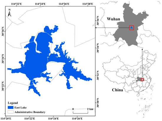
Figure 1.
Study area of East Lake in Wuhan city, China.
East Lake’s water quality is classified as Class III according to the surface water quality standards in China [23]. The background concentrations of TN, TP and COD in East Lake exceeding this standard are set at 1 mg/L, 0.2 mg/L and 20 mg/L, respectively. For NH3-N levels that do not exceed this standard, the background concentration is set at 0.15 mg/L, based on the standards of Class I.
2.2. Data Sources
2.2.1. In Situ Observation
The water quality and nutrient status of East Lake were collected and organized to obtain the inter-annual intra-annual water quality distribution maps (details in the Supplementary Materials), and the published data for the period of 2014~2022 were offered by Wuhan Municipal Bureau of Ecology and Environment (http://hbj.wuhan.gov.cn/hjsj/ (accessed on 31 March 2023)).
The present work has selected three sub-lakes, namely Xiaotan Lake (XTL), Tangling Lake (TLL) and Guozheng Lake (GZL), as sampling sites. XTL is connected to Tangling Lake, and TLL is connected to GZL through culverts or elevated bridges. The number of sampling points was determined based on the size of each sub-lake, with one sampling point for XTL, three for TLH and eight for GZL, totaling 12 sampling points. A total of 36 sets of data were collected on 10, 20 and 30 December 2021.
2.2.2. Satellite Data
The Sentinel series provides essential remote sensing data for the European Commission’s Copernicus program. The Sentinel 2 satellites are high-resolution multispectral imaging satellites divided into two spacecraft, 2A and 2B. Sentinel-2 satellite data are the only optical data that can include three bands in the red-bordered region, which is very helpful for monitoring vegetation health information. The primary purpose of Sentinel-2 is to observe global land conditions with high accuracy and resolution, supporting the mapping of physical and biological changes, and monitoring coastal and riparian dynamics. For this study, Sentinel 2 satellite image data were selected through the official website of the European Space Agency (https://www.copernicus.eu/ (accessed on 26 March 2023)) in the same steps as the measured water quality data, on 10 December 2021, 20 December 2021 and 30 December 2021, respectively.
2.3. Methods
2.3.1. Process of Water Quality Remote Sensing Inversion and Pollution Source Tracing
The following workflow outlines the methodology used to assess water quality in East Lake using satellite remote sensing and in-situ data collection. Sentinel-2 L2A-level satellite imagery was used in conjunction with measured water quality data to improve the spatial understanding of contaminant concentrations across the lake. The process involves the pre-processing of both satellite and field data, followed by regression-based water quality retrieval models. This allows the estimation of pollution sources, pollutant emission loads, and the formulation of remediation strategies. The detailed steps of this process are illustrated in Figure 2.
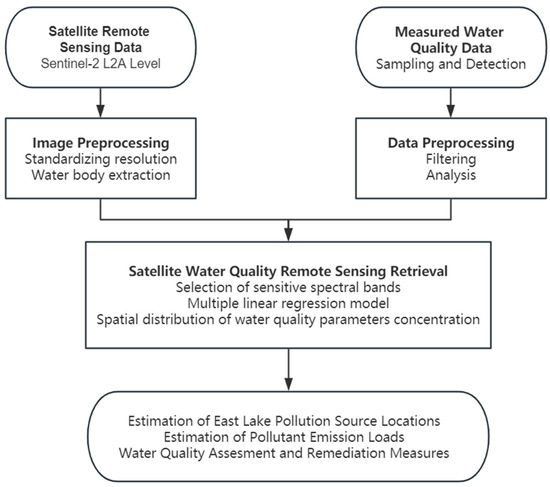
Figure 2.
Technical route illustrates the processing and comparison of remote sensing data from the Sentinel 2 Level 2A and actual water quality measurements. A multiple linear regression model is established through the selection of appropriate bands. The positions and quantities of pollution sources are determined based on the spatial concentration distribution of different water quality parameters. Recommendations for remediation are proposed based on the current state of the study area.
2.3.2. Selection of Bands
The traditional image threshold method is the most common method for water body extraction. It uses the feature that the water body has high reflectivity in some bands and low reflectivity in other parts of the bands to obtain the water body information in the image by band calculation, and extracts the water body after setting the threshold value. An adaptive extraction method based on the Normalized Difference Water Index (NDWI) is applied here to extract water completely and accurately from remote sensing images, with NDWI defined as indicated in Equation (1).
where Green and NIR represent the green band and the near-infrared band, respectively. The corresponding Sentinel-2 satellite image bands are B3 and B8.
The water quality data obtained from field sampling were tested for outliers and the data points in the samples that deviated the most from the mean were detected using the Grubbs method on SPSS. In the data analysis process, although outlier detection was initially planned, a review of the data revealed no significant outliers that required removal. Therefore, all 36 valid data for Chl-a, TN, TP, NH3-N and COD were finally obtained, of which 24 were taken for rate determination and 12 for validation.
Combined with the band settings of Sentinel 2 satellite data, Pearson correlation analysis was carried out on the correlation between the satellite data in each band and their combinations and the measured water quality index data on the ground, and the bands or combinations of bands with the strongest correlation were compared and selected.
2.3.3. Development of Multi-Regression Models
An analysis of the various factors is conducted using the Multiple Linear Regression (MLR) model. The dependent variable (target variable) is dependent on many independent variables, in this case. Using multiple linear regression model to study the quantitative relationship between dependent variables and two or more independent variables has become a widely used quantitative analysis method, as it better reflects in-situ conditions [24]. The regression equation involving multiple variables can be described as follows:
where is the predictor or target variable and are the independent variables. is the y-intercept and and are the coefficients and error term, respectively.
The selected band combinations were subjected to residual analysis with covariance determination to exclude outliers and multicollinearity between independent variables. Stepwise regression analysis was used to add independent variables into the model one by one and calculate their partial regression sum of squares. If the calculated result passes the significance test, the regression model incorporates the independent variable. At the same time, the variables already present in the model are also tested for significance and are removed from the model if they fail [25]. The linear regression models for Chl-a, TN, TP, ammonia nitrogen (NH3-N) and COD were developed using the coefficients of determination R2 of the multiple linear regression models, as an important reference index for model superiority, as shown in Appendix A.
2.3.4. Identification of the Pollution Sources
The watershed boundary of East Lake was selected according to the data provided on Google Earth, and then we used the Inverse Distance Weighted (IDW) interpolation method for generating the bathymetric map of East Lake due to its practicality and effectiveness with our dataset. The IDW method was applied to the water depth data collected from 12 measurement points across the lake. While Kriging is a more advanced geostatistical method that could offer enhanced accuracy by modeling spatial correlations, it requires a larger dataset and more complex computational resources to estimate spatial variances. Given that our dataset consisted of 12 points, IDW was chosen as it is well-suited for scenarios with limited data, offering a balance between simplicity and the level of detail required for our interpolation needs.
Due to the low flow velocity and low mobility of the lake, it can be assumed that the pollutants generated by the pollution sources at the boundary of East Lake do not spread with the water in a short period. Therefore, the concentration of the water quality parameters of the pollution source should exceed the background concentration of the surrounding water body. Based on the law of conservation of mass, the pollutants released from the pollution source are equal to the amount of pollutants degraded at that point, which can be obtained as
Divide from each side of Equation (3):
where (mg/s) is the rate of pollution from point source; (1/d) is the degradation coefficient of water quality parameter; (mg/L) is the high concentration value at the water body boundary; (mg/L) is background concentration; (L) is the volume of the water column at the selected high-concentration picture element.
With the inversion results obtained based on the remote sensing data on 10 December 2021, the spatial distribution of key water quality parameters was mapped in East Lake. Locations along the lake boundary with the highest concentrations were identified as potential pollutant discharge points. The highest concentration locations were determined by selecting the maximum pixel values along the boundary using the attribute table in ArcGIS. The principle of mass conservation was applied to link the high-concentration areas to possible pollution sources, thereby identifying the most probable discharge points. Additionally, a gradual decrease in water quality parameter concentrations from these discharge points to the surrounding areas was observed, indicating the dispersion of pollutants.
3. Results
3.1. Results of Water Surface
This study used NDWI to identify the water body of East Lake and extracted the Region of Interest (ROI) for cropping. Figure 3 shows the images before and after cropping. The bathymetric data for East Lake were processed using ArcGIS, with spatial interpolation performed via the Inverse Distance Weighting (IDW) method to obtain the underwater topography data for the entire lake. The interpolation results are illustrated in Figure 4, indicating the water depth data for the entire East Lake. From the data depicted in the Figure 4, it is observed that the maximum water depth in East Lake is approximately 4.95 m, while the minimum water depth is around 0.02 m.
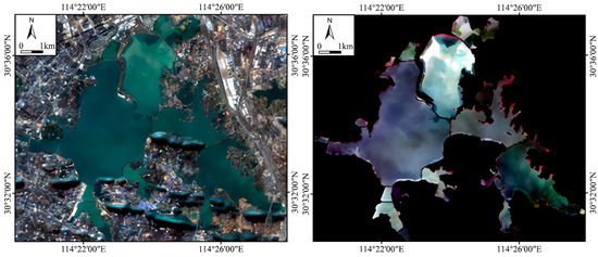
Figure 3.
Original image of East Lake water body (left) and cropped image after the extraction of water body (right).
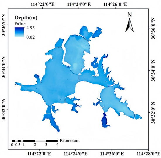
Figure 4.
The water depth of East Lake.
3.2. Multi-Regression Models for Different Index
Multiple linear regression models were established for chlorophyll-a (Chl-a), total nitrogen (TN), total phosphorus (TP), ammonia nitrogen (NH3N), and chemical oxygen demand (COD). The specific models are shown in Table 1. Based on the established model for water quality parameters, predictions were made for the validation stage data. The actual measurements and remote sensing retrieval results for both the validation and training stages were compared, as illustrated in Figure 5.

Table 1.
The multiple linear regression model for each water quality parameter and its coefficient of determination.
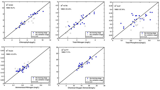
Figure 5.
Graphical fit results of the five water quality parameters (chlorophyll-a, total nitrogen, total phosphorus, ammoniacal nitrogen and chemical oxygen demand) for 10, 20 and 30 December, 1-1 line of predicted (Y) and targeted (T).
The results from the multiple linear regression models show that the majority of data points are distributed near the 1-1 standard line at the training and validation phases.
The model fitting for chlorophyll-a, total nitrogen, ammonia nitrogen and chemical oxygen demand concentrations shows satisfactory results with regression coefficients (R2) of 0.943, 0.781, 0.624 and 0.777, respectively. The predictive performance for total phosphorus is slightly inferior, with a regression coefficient (R2) of 0.489. This demonstrates that remote sensing retrieval can effectively reflect the concentrations of Chl-a, TN, TP, NH₃-N and COD. Figure 5 presents some of these graphical fit results for the five selected water quality parameters, indicating the relatively good agreement between the monitored and the simulated values and revealing that the present methodology can be used as a suitable technique to predict water quality data in East Lake.
3.3. Spatial Pattern of Remote Sensing Water Quality in Lakes
Based on the constructed multiple linear regression models for various water quality parameters, remote sensing inversion of water quality in East Lake on 10 December 2021 and 20 December 2021 was performed using ArcGIS. The results depict the spatial distribution of concentrations for Chl-a, TN, TP, NH3-N and COD, as indicated in Figure 6.
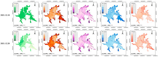
Figure 6.
The concentration distribution of the five water quality parameters (chlorophyll-a, total nitrogen, total phosphorus, ammoniacal nitrogen and chemical oxygen demand) on 10 December and 20 December 2021.
3.4. Pollution Patterns
With the inversion results obtained based on the remote sensing data on 10 December 2021, the location of possible pollution sources on the boundary can be inferred. Comparing the obtained East Lake bathymetric data with the previously acquired dataset, depths corresponding to potential pollution source locations were identified. Subsequently, the concentrations of pollutants at these source locations were calculated (see Table 2 and Figure 7).

Table 2.
Estimated locations of potential pollution sources for each water quality indicator along with the discharged pollutant quantities.
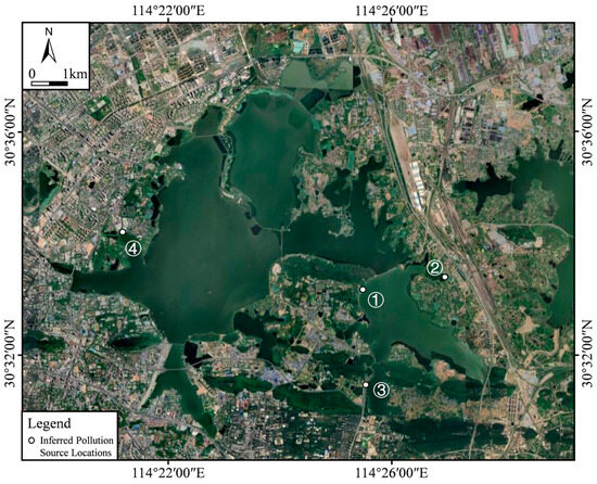
Figure 7.
Locations of potential discharge pollution for various water quality indicators in East Lake.
The information table of the outfalls of each sub-lake in East Lake was downloaded from the official website of the Wuhan Ecological and Environmental Protection Bureau (WEPB), and excerpts of some of the outfalls of Hou Lake (HL), Yujia Lake (YJL) and Tiane Lake (TEL) are shown in Table S1.
The highest emissions of total nitrogen and total phosphorus occur in the posterior lake area, with the highest ammonia nitrogen emissions observed in Yujia Lake. Chemical oxygen demand has the highest emissions in the Tiane Lake area.
Upon comparing the coordinates in Table S1, it becomes apparent that the locations of the four potential pollution sources (① to ④ in Table 2 and Figure 7) are associated with nearby outfalls. Specifically, point 1 is located near outfall number 217. The presumed pollution source at point 2 lies between outfalls 126 and 128. Additionally, the presumed pollution source at point 3 is in proximity to outfall 198, and the presumed pollution source at point 4 is flanked by outfalls 408 and 409. Figure 8 presents a visual comparison between the officially disclosed locations of East Lake outfalls (marked in red) and the presumed pollution source positions estimated in this study (marked in white). The observation that each of the four presumed pollution source locations is surrounded by stormwater and wastewater outfalls indicates the applicability of this method for inferring pollution source locations.
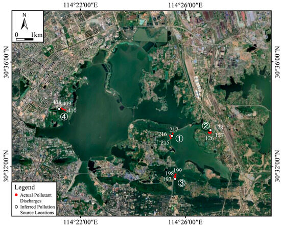
Figure 8.
Comparison between the actual pollutant discharges in East Lake and the inferred pollution source locations.
4. Discussion
The spatial distribution of water quality parameters obtained through remote sensing inversion, as shown in Figure 6, closely corresponds to prior research findings in East Lake. In general, nitrogen and phosphorus concentrations in East Lake surpass standard limits. The southern part of East Lake exhibits relatively poorer water quality compared to the northern part. Concentration trends for Chl-a, TN, TP and NH3-N are generally consistent, with the central regions of large sub-lakes in East Lake, such as Guozheng Lake (GZL), Tangling Lake (TLH) and Tuan Lake (TL), showcasing relatively better water quality. Conversely, peripheral smaller sub-lakes like Yujia Lake (YJL) and Miao Lake (ML) demonstrate relatively poorer water quality due to limited water exchange [26]. The distribution trend of COD concentration deviates from other indicators, with lower COD concentrations observed in YJL and ML. Areas near East Lake sewage outlets, regions with frequent human activities and enclosed small sub-lakes with poor water mobility exhibit poorer water quality conditions. These findings align with the regional eutrophication status reported on the official website of the Wuhan Municipal Ecology and Environment Bureau (Table S1). And they are also consistent with previous research findings that higher concentrations of Chl-a are commonly observed in sub-lakes such as Yujia Lake, Tuan Lake, Miao Lake and Shuiguo Hu [27]. Notably, Chl-a levels are higher near the edges of these lakes, close to the land, compared to the central regions of the lakes [28]. Li et al. [29] utilized Landsat-8 images and measured data to construct a MIKE 21 model and similarly investigated chlorophyll-a concentrations in East Lake. Their findings indicated that chlorophyll-a concentrations were generally poorer near the periphery of the southwest bank of East Lake, with water quality gradually improving toward the central area of the lake. This study’s results are consistent with these results, further confirming the spatial patterns of water quality distribution in East Lake.
Zhang et al. [30] used Landsat TM/ETM+ and OLI imagery to predict water quality parameters in Danjiangkou Reservoir, and the coefficients of determination R2 for total nitrogen and chemical oxygen demand were 0.62 and 0.61, respectively, during the dry season. For this study, using Sentinel-2 data and a multiple linear regression model achieved higher R2 values for the same two water quality parameters (R2 > 0.75). This suggests that the remote sensing approach used in this study is effective in capturing water quality variations, particularly when compared to similar methodologies in other studies. However, as both studies indicate, the performance of regression models may vary depending on the specific water quality parameters and the characteristics of the study area, highlighting the need for further research across different temporal and spatial scales.
The proximity of stormwater and wastewater outfalls to each of the four identified potential pollution sources, as shown in Figure 8, demonstrates the effectiveness of this method in pinpointing pollution source locations. This finding demonstrates the potential utility of our model in identifying areas with elevated pollution risks, supporting its broader application in similar contexts.
After analyzing the water quality data for Chl-a, TN, TP, NH₃-N and COD, it was determined that there were no significant outliers that required removal. It is important to note that the handling of outliers can significantly impact the conclusions drawn from a small dataset.
From the remotely sensed concentration of water quality parameters in this study, it is evident that East Lake faces water pollution issues in the year 2021, often falling short of the planned Class III water quality standards. Despite increased efforts by the Wuhan municipal government to address pollution in East Lake, the water quality has frequently reached Class V conditions in recent years, as presented in Figure S1. During the investigation of East Lake outfalls, a significant amount of industrial and domestic wastewater discharge into the lake was observed. Although the treated discharged wastewater meets standards, the cumulative volume still exceeds the water environmental capacity of East Lake.
However, there are still many limitations to this study that require further exploration and validation in future research.
First, due to the lack of long-term data, the measured data in this study primarily reflect the water quality conditions of East Lake during the winter of 2021, which is not comprehensive enough to represent the conditions in other seasons or years. Additionally, the time scale for simulation and prediction is relatively short. With more extensive water quality data, future research can conduct a more thorough analysis of the spatial and temporal variations in East Lake’s water quality over an extended period. This would allow for a comparison of water quality across different seasons and enable long-term predictions on an annual scale, helping to identify the factors influencing changes in East Lake’s water quality.
Secondly, the satellite-based remote sensing approach used in this study is limited to assessing the uppermost part of the water column, and thus may not fully represent the vertical stratification of the water body. We did not consider the effects of hydrodynamic processes within East Lake, such as hydrodynamic mixing, eddies and water circulation patterns, which can influence the distribution of pollutants. These processes may cause pollutants to disperse and accumulate in areas that do not directly correspond to their source, potentially leading to inaccuracies in pinpointing discharge locations. In addition, factors such as water, grass and sediment can affect spectral data and, consequently, the identification of pollution sources. To address these limitations in future studies, incorporating hydrodynamic modeling alongside remote sensing data would be beneficial. By simulating water flow and mixing patterns within the lake, we could more accurately trace the movement of pollutants from their source to their observed concentrations. Future studies should consider removing pixels from areas near the shore or aquatic zones to enhance the accuracy of the results. Additionally, including data from different depths and integrating in situ measurements could improve our understanding of subsurface discharges and their impact on water quality.
5. Conclusions
This study focuses on East Lake in Wuhan and involves constructing a remote sensing inversion model based on satellite imagery and concurrently collected water quality data. The model is used to infer the spatial distribution of water quality indicators. The accuracy and simulation performance of the model are evaluated by comparing its results with actual water quality data from sampled points. Assessing the distribution of water quality indicators makes it possible to identify regions with elevated concentrations along the boundaries, enabling the determination of potential pollution sources and the calculation of pollutant discharge. Verification is conducted by comparing these findings with the actual discharge points in East Lake. Remote sensing technology is utilized for water quality monitoring in East Lake, and an efficient water quality prediction model is developed.
The multiple linear regression model provided a good relationship between the observed and simulated water quality parameters, with four parameters correlated at R2 > 0.6 and the remaining one correlated at R2 > 0.45. The result shows that the location of the main pollution sources for the inferred water quality parameters was close to the publicly disclosed discharge point. This method can be applied to lakes where the discharge point locations are unknown. A longer period should be investigated to test the multiple linear regression model, determine its performance and assess the impacts of East Lake restoration on water quality parameters.
Considering the analyzed concentration distribution results of remotely sensed parameters in various sub-lakes of East Lake, issues with the current water quality status are identified, such as non-compliance with water quality standards and the frequent occurrence of “algae bloom”. In response to these problems, several remediation recommendations are proposed.
5.1. Improvement in East Lake Water System Structure
Although the “Grand East Lake Water Network Connection Project” was initiated by the Wuhan municipal government in 2009, effectively managing water quality parameters in the large sub-lakes of East Lake, some of the smaller sub-lakes in its vicinity still experience poor water circulation. These smaller sub-lakes are significantly influenced by pollution discharges from surrounding enterprises and human activities. Beyond the existing culverts and sluice gates, enhancing connectivity between the sub-lakes could be considered to improve the self-purification capacity of the water body in East Lake.
5.2. Management of Pollution Sources in East Lake
To tackle the increased pollution in the southern and nearshore areas of East Lake, it is essential to enhance the redevelopment of adjacent sewage treatment plants. This includes expanding the sewage treatment capacity to accelerate the purification of water. Furthermore, a centralized approach for treating pollutants from urban sewage and aquaculture is imperative.
5.3. Enhancement of the Construction Supervision System
The water protection authority responsible for East Lake should actively disseminate information by consistently consolidating and publishing monthly water quality monitoring data on its official website. This initiative aims to uphold transparency, enabling easy public access to crucial water quality information. By involving the community in overseeing the water conditions of East Lake, a collaborative partnership between the government and the public can be established.
Utilizing remote sensing inversion data for East Lake, we inferred potential discharge points. Four locations, characterized by the highest pollutant concentrations with a subsequent decrease in surrounding water bodies, were designated as potential pollution sources. A comparative analysis with publicly available information on East Lake’s discharge points confirmed a reasonable alignment, showcasing the utility of the remote sensing inversion model in pinpointing pollutant source locations. This significantly enhances the model’s potential application to other water bodies.
In conclusion, this model can subsequently be applied to broader watershed studies, including the Yangtze River, for improved assessment of water quality conditions. This approach holds scientific significance and practical value in enhancing water environmental management and remediation efforts.
Supplementary Materials
The following supporting information can be downloaded at: https://www.mdpi.com/article/10.3390/rs16183402/s1.
Author Contributions
Methodology, S.H. and Y.Z.; Data curation, S.H. and Y.Z.; Writing—original draft, S.H. and Y.Z.; Writing—review & editing, L.L. and Y.S. All authors have read and agreed to the published version of the manuscript.
Funding
This research was funded by National Natural Science Foundation of Joint Fund for Changjiang River Water Science Research, grant number U2340201.
Data Availability Statement
The products used in this study are publicly available as follows: The Sentinel 2 satellite image data presented in the study can be accessed via https://www.copernicus.eu/ (accessed on 31 March 2023). The nutrient status of East Lake can be accessed via http://hbj.wuhan.gov.cn/hjsj/ (accessed on 31 March 2023). The raw data supporting the conclusions of this article will be made available by the authors on request.
Acknowledgments
The subject of this paper is derived from the 2022 Major Science and Technology Project of the Ministry of Water Resources: “Key Technologies for Operation and Control of Water Conservancy Satellite Constellation and Applications”, and “Collaborative Research and Development of Luojia-2 (Guangyin-2) 01 Satellite”. The authors thank the supervisors Yanjun Zhang at Wuhan University and Hong Zhang at Griffith University for their support.
Conflicts of Interest
The authors declare no conflict of interest.
Appendix A. Selection of Bands

Table A1.
The spectral bands utilized in this study to the absence of Band 10 data in Level 2A imagery.
Table A1.
The spectral bands utilized in this study to the absence of Band 10 data in Level 2A imagery.
| Band Number | Band Name | Center Wavelength (nm) | Bandwidth (nm) | |
|---|---|---|---|---|
| B1 | Band 1 | Coastal | 443 | 20 |
| B2 | Band 2 | Blue | 490 | 65 |
| B3 | Band 3 | Green | 560 | 35 |
| B4 | Band 4 | Red | 665 | 30 |
| B5 | Band 5 | Red Edge1 | 705 | 15 |
| B6 | Band 6 | Red Edge2 | 740 | 15 |
| B7 | Band 7 | Red Edge3 | 783 | 20 |
| B8 | Band 8 | NIR | 842 | 115 |
| B9 | Band 8A | Red Edge4 | 865 | 20 |
| B10 | Band 9 | Water vapor | 945 | 20 |
| B11 | Band 11 | SWIR-1 | 1610 | 90 |
| B12 | Band 12 | SWIR-2 | 2190 | 180 |
Considering the band configuration of Sentinel-2 data, Pearson correlation analysis was conducted using the correlation analysis tools in SPSS software. This analysis aimed to assess the correlation between various satellite bands or their combinations and ground-measured water quality indicators. Recent domestic and international research on water quality remote sensing has suggested that models derived from feature bands with strong correlations to water quality parameters yield higher accuracy than single-band models [31]. Therefore, a total of 342 band combinations were explored by adding, subtracting, multiplying and dividing the participating bands. The correlation coefficients between these 342 band combinations and the five water quality indicators in this study (Chl-a, TN, NH3-N, TP and COD) are presented in Table A2, Table A3, Table A4, Table A5 and Table A6, highlighting the band combinations with significant correlations.

Table A2.
Correlation between Chl-a and spectral bands (combinations).
Table A2.
Correlation between Chl-a and spectral bands (combinations).
| Bands (Combinations) | Correlation Coefficient R |
|---|---|
| B8–B11 | 0.876 ** |
| B8 | 0.864 ** |
| B1 * B8 | 0.863 ** |
| B8 + B12 | 0.862 ** |
| B7 + B8 | 0.859 ** |
| B6 + B8 | 0.858 ** |
| B1 + B8 | 0.856 ** |
| B8–B12 | 0.856 ** |
| B8 + B9 | 0.855 ** |
| B6–B11 | 0.855 ** |
| B7–B11 | 0.855 ** |
| B1 * B7 | 0.855 ** |
| B5 * B9 | 0.855 ** |
| B7 * B8 | 0.855 ** |
| B1 + B7 | 0.853 ** |
| B1 * B6 | 0.853 ** |
| B6 * B8 | 0.853 ** |
Significance levels: ** p < 0.01.

Table A3.
Correlation between TN and spectral bands (combinations).
Table A3.
Correlation between TN and spectral bands (combinations).
| Bands (Combinations) | Correlation Coefficient R |
|---|---|
| B1–B6 | −0.752 ** |
| B1–B5 | −0.676 ** |
| B3–B5 | −0.661 ** |
| B1–B7 | −0.653 ** |
| B2–B5 | −0.641 ** |
| B3–B4 | −0.624 ** |
| B1/B5 | −0.619 ** |
| B5/B1 | 0.617 ** |
| B2–B6 | −0.600 ** |
| B2–B7 | −0.572 ** |
| B2/B5 | −0.550 ** |
| B5/B2 | 0.548 ** |
| B1–B8 | −0.532 ** |
| B1–B8A | −0.524 ** |
| B8A/B9 | 0.515 ** |
Significance levels: ** p < 0.01.

Table A4.
Correlation between NH3-N and spectral bands (combinations).
Table A4.
Correlation between NH3-N and spectral bands (combinations).
| Bands (Combinations) | Correlation Coefficient R |
|---|---|
| B6–B8A | 0.592 ** |
| B8–B8A | 0.570 ** |
| B6–B7 | 0.554 ** |
| B1–B2 | 0.503 ** |
| B2/B6 | −0.495 ** |
| B1/B2 | 0.495 ** |
| B8–B11 | 0.489 ** |
| B2/B1 | −0.487 ** |
| B2/B8 | −0.478 ** |
| B9/B8A | 0.476 ** |
Significance levels: ** p < 0.01.

Table A5.
Correlation between TP and spectral bands (combinations).
Table A5.
Correlation between TP and spectral bands (combinations).
| Bands (Combinations) | Correlation Coefficient R |
|---|---|
| B2–B8 | −0.480 ** |
| B2–B9 | −0.460 ** |
| B2–B7 | −0.421 * |
| B2–B8A | −0.414 * |
| B2–B12 | −0.393 * |
| B2–B6 | −0.392 * |
| B1–B9 | −0.391 * |
| B1–B8 | −0.388 * |
| B2 * B3 | −0.384 * |
| B2–B11 | −0.382 * |
Significance levels: * p < 0.05, ** p < 0.01.

Table A6.
Correlation between COD and spectral bands (combinations).
Table A6.
Correlation between COD and spectral bands (combinations).
| Bands (Combinations) | Correlation Coefficient R |
|---|---|
| B4–B8 | 0.598 ** |
| B4–B8A | 0.578 ** |
| B4–B9 | 0.564 ** |
| B4–B6 | 0.542 ** |
| B4–B7 | 0.534 ** |
| B4–B11 | 0.528 ** |
| B3 * B12 | 0.517 ** |
| B3 * B4 | 0.509 ** |
| B4 * B12 | 0.508 ** |
| B4 + B12 | 0.506 ** |
| B3 + B12 | 0.501 ** |
| B3 + B4 | 0.500 ** |
| B4 | 0.499 ** |
Significance levels: ** p < 0.01.
The concentrations of TN, TP and NH₃-N show a predominantly negative correlation with band combinations, while Chl-a and COD concentrations exhibit predominantly positive correlations with band combinations. The relationship between Chl-a concentration in East Lake and various band combinations is particularly strong, with many correlation coefficients exceeding 0.85. TN, NH₃-N and COD exhibit moderate correlations with band combinations, reaching values above 0.5. However, the correlation between TP and band combinations is relatively weak, with only a few combinations exceeding 0.4. Notably, the band combination B8-B11 shows the highest correlation with Chl-a, B1-B6 with TN, B6-B8A with NH₃-N, B2-B8 with TP and B4-B8 with COD. These strong correlations suggest the potential for constructing multiple linear regression models using band combinations to predict water quality indicators.
References
- Xie, H.; Tong, X. Remote sensing applications in water quality monitoring and assessment. Remote Sens. Inf. 2006, 2, 67–70+75. [Google Scholar] [CrossRef]
- Kallio, K. Remote sensing as a tool for monitoring lake water quality. In Water Quality Measurements Series: Hydrological and Limnological Aspects of Lake Monitoring; John Wiley & Sons: Hoboken, NJ, USA, 2007. [Google Scholar]
- Zhou, Y.; Zhou, W.; Wang, S.; Zhang, B. Application of remote sensing technology in inland water quality monitoring. Adv. Water Sci. 2004, 15, 312–317. [Google Scholar]
- Ma, R.; Tang, J. Acquisition and algorithm analysis of lake water color remote sensing parameters. Adv. Water Sci. 2006, 17, 720–726. [Google Scholar]
- Kloiber, S.M.; Brezonik, P.L.; Olmanson, L.G.; Bauer, M.E. A procedure for regional lake water clarity assessment using Landsat multispectral data. Remote Sens. Environ. 2002, 82, 38–47. [Google Scholar] [CrossRef]
- Cheng, S.; Zhang, S.; Zhao, K. Biological water quality monitoring method based on convolutional neural network. J. Metrol. Soc. 2019, 40, 721–727. [Google Scholar]
- Xiao, J.; Zhou, X.; Pan, Y.; Feng, W.; Chen, D. Application of GA-BP optimized TS fuzzy neural network in water quality monitoring and evaluation system prediction model—Taking Taihu Lake as an example. J. Southwest Univ. (Nat. Sci. Ed.) 2019, 41, 110–119. [Google Scholar]
- Guan, J. Application of Support Vector Machine in Fusion and Evaluation of Water Quality Monitoring Information. Ph.D. Thesis, Hohai University, Nanjing, China, 2006. [Google Scholar]
- Li, S.; Xu, H.; Wang, L. Remote sensing analysis of suspended particles in coastal waters. Remote Sens. Technol. Appl. 2005, 20, 601–605. [Google Scholar] [CrossRef]
- Xing, X.; Shen, Q.; Li, J.; Zhang, F.; Pang, Z.; Lü, S. Remote sensing inversion of river suspended sediment concentration in Manwan Dam area based on HJ-CCD. Remote Sens. Technol. Appl. 2016, 31, 682–690. [Google Scholar]
- Kuang, Q.; Xia, Y.; Li, Z.; Zhuang, D.; Liu, B.; Zhan, F. Aquatic organisms and aquatic function in different nutrient types of sub-lakes in Donghu, Wuhan. J. Lake Sci. 1997, 9, 249–254. [Google Scholar]
- Hoogenboom, H.J.; Dekker, A.G.; de Haan, J.F. Retrieval of chlorophyll and suspended matter from imaging spectrometry data by matrix inversion. Can. J. Remote Sens. 1998, 24, 144–152. [Google Scholar] [CrossRef]
- Li, S.; Wang, X. Spectral characteristics and quantitative remote sensing of inland water quality parameters. Geogr. Territ. Res. 2002, 18, 26–30. [Google Scholar]
- Zhu, L.; Li, Y.; Zhao, S.; Guo, Y. Remote sensing monitoring of water quality in Taihu Lake based on GF-1 satellite WFV data. Remote Sens. Land Resour. 2015, 27, 113–120. [Google Scholar]
- Carlson, R.E. A trophic state index for lakes. Limnol. Oceanogr. 1977, 22, 361–369. [Google Scholar] [CrossRef]
- Wang, X.; Sun, S. Study on monitoring of river water quality based on TM and ANN. Chin. J. Environ. Eng. 2009, 3, 1532–1536. [Google Scholar]
- Xu, Y.; Zhang, Y.; Chen, H.; Zhang, D. Remote sensing monitoring of soluble inorganic nitrogen concentration in Haizhou Bay based on MODIS. Adv. Mar. Sci. 2011, 29, 73–80. [Google Scholar]
- Lillesand, T.M.; Johnson, W.L.; Deuell, R.L.; Lindstrom, O.M.; Meisner, D.E. Use of Landsat data to predict the trophic state of Minnesota lakes. Photogramm. Eng. Remote Sens. 1983, 49, 219–229. [Google Scholar]
- Lathrop, R.G.; Lillesand, T.M.; Yandell, B.S. Testing the utility of simple multi-date thematic mapper calibration algorithms for monitoring turbid inland waters. Int. J. Remote Sens. 1991, 12, 2045–2063. [Google Scholar] [CrossRef]
- Rodríguez-Molina, J.J.; García-Martínez, R. Hydrotrack: A graphical software system for the simulation of pollutant discharges in water. Environ. Model. Softw. 1998, 13, 211–223. [Google Scholar] [CrossRef]
- Richards, S.; Withers, P.J.; Paterson, E.; McRoberts, C.W.; Stutter, M. Potential tracers for tracking septic tank effluent discharges in watercourses. Environ. Pollut. 2017, 228, 245–255. [Google Scholar] [CrossRef]
- Liu, J.; Huang, X. Overview of ecological research on Donghu. Environ. Sci. 1997, 18, 51–53. [Google Scholar]
- GB 3838-2002; Surface Water Environmental Quality Standards. China Environmental Publishing Group: Beijing, China, 2019.
- Guo, Y.; Li, Y.; Li, Y.; Lü, H.; Liu, G.; Wang, X.-D.; Zhang, S.-M. A three-band estimation model of chlorophyll-a concentration based on GOCI data. Environ. Sci. 2015, 36, 3175–3185. [Google Scholar]
- Cong, S. Theory and Application of Neural Network for MATLAB Toolbox; China University of Science and Technology Press: Beijing, China, 2009. [Google Scholar]
- Yu, C.; Ren, X.; Ban, X.; Zhang, L.; Du, Y. Study on the spatial distribution characteristics of nitrogen in typical shallow lakes in Hubei Province in winter—Taking Honghu and Donghu in Wuhan as examples. J. Cent. China Norm. Univ. (Nat. Sci. Ed. ) 2011, 45, 490–496. [Google Scholar]
- Bai, K. Monitoring and Evaluation System of Lake Eutrophication Based on 3S Technology. Ph.D. Thesis, Huazhong University of Science and Technology, Wuhan, China, 2019. [Google Scholar]
- Yang, X.; Jiang, Y.; Deng, X.; Zheng, Y.; Yue, Z. Temporal and spatial variations of Chlorophyll a concentration and eutrophication assessment (1987–2018) of Donghu Lake in Wuhan using Landsat images. Water 2020, 12, 2192. [Google Scholar] [CrossRef]
- Li, X.; Huang, M.; Wang, R. Numerical simulation of Donghu Lake hydrodynamics and water quality based on remote sensing and MIKE 21. ISPRS Int. J. Geo-Inf. 2020, 9, 94. [Google Scholar] [CrossRef]
- Zhang, Y.; Huang, X.; Yin, W.; Zhu, D. Multitemporal landsat image based water quality analyses of Danjiangkou Reservoir. Photogramm. Eng. Remote Sens. 2017, 83, 643–652. [Google Scholar] [CrossRef]
- Zhang, J.; Li, Y. Research on sensor situation based on multiple linear regression prediction model. Comput. Technol. Dev. 2011, 21, 229–232. [Google Scholar]
Disclaimer/Publisher’s Note: The statements, opinions and data contained in all publications are solely those of the individual author(s) and contributor(s) and not of MDPI and/or the editor(s). MDPI and/or the editor(s) disclaim responsibility for any injury to people or property resulting from any ideas, methods, instructions or products referred to in the content. |
© 2024 by the authors. Licensee MDPI, Basel, Switzerland. This article is an open access article distributed under the terms and conditions of the Creative Commons Attribution (CC BY) license (https://creativecommons.org/licenses/by/4.0/).