Article

On Connecting Hydrosocial Parameters to Vegetation Greenness Differences in an Evolving Groundwater-Dependent Ecosystem

by
Matthew R. Lurtz
1,2,*,
Ryan R. Morrison
3 and
Pamela L. Nagler
4
1
Department of Geosciences, Colorado State University, Fort Collins, CO 80523, USA
2
Cooperative Institute for Research in Environmental Sciences, University of Colorado, Boulder, CO 80309, USA
3
Department of Civil and Environmental Engineering, Colorado State University, Fort Collins, CO 80523, USA
4
U. S. Geological Survey, Southwest Biological Science Center, University of Arizona, Tucson, AZ 85719, USA
*
Author to whom correspondence should be addressed.
Remote Sens. 2024, 16(14), 2536; https://doi.org/10.3390/rs16142536
Submission received: 29 April 2024 / Revised: 14 June 2024 / Accepted: 29 June 2024 / Published: 10 July 2024
(This article belongs to the Special Issue Monitoring Ecohydrology with Remote Sensing)

Abstract

:
Understanding groundwater-dependent ecosystems (i.e., areas with a relatively shallow water table that plays a major role in supporting vegetation health) is key to sustaining water resources in the western United States. Groundwater-dependent ecosystems (GDEs) in Colorado have non-pristine temporal and spatial patterns, compared to agro-ecosystems, which make it difficult to quantify how these ecosystems are impacted by changes in water availability. The goal of this study is to examine how key hydrosocial parameters perturb GDE water use in time and in space. The temporal approach tests for the additive impacts of precipitation, surface water discharge, surface water mass balance as a surrogate for surface–groundwater exchange, and groundwater depth on the monthly Landsat normalized difference vegetation index (NDVI). The spatial approach tests for the additive impacts of river confluences, canal augmentation, development, perennial tributary confluences, and farmland modification on temporally integrated NDVI. Model results show a temporal trend (monthly, 1984–2019) is identifiable along segments of the Arkansas River at resolutions finer than 10 km. The temporal impacts of river discharge correlate with riparian water use sooner in time compared to precipitation, but this result is spatially variable and dependent on the covariates tested. Spatially, areal segments of the Arkansas River that have confluences with perennial streams have increased cumulative vegetation density. Quantifying temporal and spatial dependencies between the sources and effects of GDEs could aid in preventing the loss of a vulnerable ecosystem to increased water demand, changing climate, and evolving irrigation methodologies.

Graphical Abstract

1. Introduction

Groundwater-supported ecosystems are under threat from the changing climate and human encroachment in the form of land-use change and agriculture [1]. Groundwater-dependent ecosystems (GDEs), or riparian ecosystems, like the ecosystems along the Arkansas River in southeastern Colorado, USA, can be measured to identify shared hydrologic connections between managed surface water and the adjacent agricultural landscape [2]. This research focuses on terrestrial vegetation, referred to here as GDE and riparian, because it is an ecosystem that (a) naturally emerges near the river bank, (b) relies on groundwater for water requirements (b), and meets the third type of classification (i.e., terrestrial vegetation as opposed to aquatic) of a GDE as summarized by Eamus et al. (2006) [3,4]. Understanding the interconnections between an agro-ecosystem (i.e., human-modified area used for production of crops) and a riparian ecosystem can improve the conjunctive management of groundwater and surface water [5]. The research dissecting the interconnections between riparian ecosystems and the surrounding landscape are plentiful. Previous research has emphasized applications like the numerical modeling of groundwater and surface water flow [5,6,7,8,9], theoretical with stochastic modeling [10,11], and a plethora of geospatial approaches [12,13,14,15] that utilize satellite imagery all to quantify the sources and effects for groundwater-dependent ecosystems. Groundwater plays a critical role supplying water for terrestrial vegetation that, in turn, provides ecosystem services like migratory bird habitats, water purification, and soil accumulation [16].
The background on quantifying the connectivity between an irrigated landscape and riparian water use is incomplete [17]. There are little data about the temporal impact of irrigation-perturbed return flow on riparian water use. Temporal lags and spatial dependencies between the source (i.e., water supply) and effect (i.e., riparian water use) should be examined to prevent the loss of a vulnerable ecosystem to increased water demand, changing climate, and evolving irrigation methodologies. Temporal lag refers to the relationship between two variables at earlier times. Floodplain activity in southeastern Colorado consists of flood-furrow irrigation of agricultural crops with a portion of land that utilizes center-pivot and drip technology [18]. Flooding as an irrigation method, as opposed to center-pivot, can cause spatially dependent increases in surface–groundwater exchange [7]. A review of groundwater recharge measurement methodologies by Scanlon, Healy, and Cook (2002) shows irrigating activity can contribute a large portion of water to return flow (i.e., from groundwater to surface water body) [19]. Recently, a global synthesis of recharge data indicates that groundwater plays a larger role than previously thought in controlling streamflow and evapotranspiration (ET) [20]. In turn, locations along the riparian corridor that are in the path of irrigation-perturbed exchange flows can depend on the extra flow as a water source [5]. Relevant research estimates 50% of the water applied to agricultural areas in the Arkansas River basin is converted to return flow [21,22], and irrigation-altered return flows are connected to riparian ecology along the Arkansas River in Colorado [23].
Two unique layers of complexity to the water balance in southeastern Colorado consist of a process known as canal augmentation and the influx of non-native vegetation. Canal augmentation occurs when a water user (e.g., farmer) has switched from flood-furrow practices to center-pivot irrigation. The Arkansas River then receives augmentation water, in timing and amount, that would have occurred if the water user still required water from a canal [24]. The augmentation water prevents changes in historic stream hydrology when irrigation methods change [24]. The dual impact of canal augmentation and irrigation methodology changes on GDE response (i.e., ET or vegetation density changes) are not well understood. Similar to river systems in western USA, non-native species like saltcedar (Tamarix ramosissima, also known as tamarisk or tamarix) grow unfettered given their ability to withstand high temperatures and salt-laden soils [23,25,26,27,28,29]. Saltcedar growth is more dependent on groundwater than precipitation, which has water use implications in an irrigated river valley with groundwater reliance [30]. The research presented here examines key human-influenced hydrologic factors (i.e., hydrosocial) on GDE vegetation patterns to draw inferences on green vegetation abundance due to water supply. Exchange flow and return flow exist across many spatial and temporal scales [31]. We use both terms interchangeably in this research because the methodology applied in the time series approach examines irrigation-altered exchange flows from a near-river perspective (i.e., upstream to downstream mass balance), and the spatial analysis examines which floodplain characteristics can provide inference on the presence of return flow using point and non-point source data (i.e., confluence location and irrigation methodology change).
We use publicly available data, cloud computing capabilities, and Bayesian techniques to examine the spatial and temporal dependencies of riparian vegetation health [32]. The models applied in this study deal with lagged covariates and autoregressive (AR) signatures and are used in economic, hydrologic, and ecological studies to understand data and make predictions [33,34,35,36,37,38]. Lagged temporal regression (e.g., estimation of dependence on factors at earlier times) is appropriate for examining GDE vegetation greenness because the state of the ecosystem at a given time could be due to past inputs into the watershed [5,39]. Spatial regression combined with categorical covariates can test hypotheses about the connections between floodplain activity and GDEs [40]. A family of Bayesian linear regression models are used to investigate patterns of vegetation over time and space. Linear models are used because advanced applications of remote sensing of ET have linear functional forms [41,42,43], and though the underlying mechanisms that connect human-made and natural ecosystems are complex, applying linear models is a necessary step in understanding spatio-temporal processes [44].
This research evaluates what temporal and spatial statistical models can uncover about the connections between natural ecosystem biomass, as a surrogate for water use, and the adjacent landscape and if the findings agree with previous studies. The following hypotheses are addressed: (1) a temporal trend in monthly normalized difference vegetation index (NDVI) covering the riparian vegetation along the Arkansas River is only detectable at spatial scales smaller than catchment (10 km), (2) the time lag of monthly NDVI with precipitation is shorter than that with river discharge, (3) riparian areas along the Arkansas River that intersect with perennial streams have increased cumulative vegetation density compared to other floodplain characteristics examined (e.g., agriculture transition to fallow). The first hypothesis is useful to determine if the spatial scale at which temporal trend is identifiable (i.e., identifying ecosystem change) is spatially relevant to the scale at which the Arkansas River is managed. This hypothesis has implications for the co-management of water supply and ecosystem sustainability. The second hypothesis is useful in separating the timing of inputs to the GDE. This hypothesis has implications for management action, like environmental flows (i.e., managed surface water input) to support GDE function. The third hypothesis associates floodplain characteristics with GDE response to inform resource managers on the connectivity between two ecosystems. These hypotheses are proposed to deduce the hydrosocial connections between human-built and natural ecosystems to inform decision making at operational scales. The analysis conducted herein tests these hypotheses using a time series modeling approach, previously used to highlight the connections between vegetation life cycles and various external forcing [13,35,45,46,47,48] and a spatial modeling approach with Gaussian-process regression techniques that has been previously used on spatial data problems to account for spatial random effects between similar regions [44,49,50].

2. Materials and Methods

2.1. Study Area

The GDE under examination borders a 96 km segment of the Arkansas River in southeastern Colorado with an areal coverage of 52.5 km2. Figure 1 depicts the study area that begins downstream of the John Martin Reservoir near Lamar, Colorado, and extends to the Colorado–Kansas border. The climate is semiarid with rainfall ranging from 343 mm to 394 mm [24]. We demarcated the extents of the GDE using Google’s platform of satellite imagery (varies upon resolution) and a series of past cropping-pattern extents from the National Land Cover Database collected in 2001 and 2016 [32].

2.2. The Landsat Data and Strategic Spatial Partitioning

Using Google Earth Engine (GEE), all Landsat 5, 7, and 8 imagery (path: 31 and row: 34) from 1984–2019 are used to extract NDVI for the study area [32]. The NDVI product is used in this study to track biomass, as a proxy for ET, due to the history the product has as an effective parameter in satellite-based ET algorithms [41,53] and because NDVI has been validated in tracking groundwater-dependent ecosystems [14,54,55]. In total, data from 932 satellites are used. Each satellite pixel (30 m) centroid that falls within the areal extent of the riparian corridor is defined as a sampling point to extract values of surface-reflected NDVI from each satellite scene. This sampling scheme resulted in a total of 58,443 satellite pixels covering the study area. All imagery is screened for clouds, ice, and cloud shadows within the areal extent of the riparian corridor. We follow the same methodology as Albano et al. (2020) using a built-in GEE algorithm that combines image metadata and spectral reflectance data to mask-out erroneous pixel values [12,32]. Following Hungtington et al. (2016), Landsat 8 Operation Land Imager data are linearly corrected for comparison with Landsat 5 and 7 [14]. The data are exported into R to be organized [56]. All pixel values found in error, likely due to the presence of clouds or snow and scan line corrector error, are assigned an NA value. Points that fall within the water surface area of the Arkansas River are removed using the National Land Cover Database Open Water classification [57]. All satellite pixels are divided into areal plots, hereafter referred to as subregions, based on the location of the satellite pixel along the Arkansas River. The landward extent of each sub-region is defined by past and present crop-patterning extents and varies between ten to hundreds of meters. Table 1 provides a summary of the subregions within the study area. The subregions in this study correspond to areas with eight distinct hydrologic response functions as defined by the rainfall-runoff model that Colorado’s Division of Water Resources (DWR) uses to model sections of the Arkansas River with the Hydrologic Institutional Model to ensure compliance with the Arkansas River Compact between Colorado and Kansas [58].

2.2.1. Temporal Representation of NDVI

Each sub-region is represented as a time series vector with dimensions of T = 428 × 1 , where T is the length of the time series in months. Each value in the vector is the average monthly NDVI ranging from May 1984 to December 2019. Subregions ( d = 1 , , D = 8 ) represent the number of separate time series vectors created for the entire study area. Monthly NDVI is computed at the Landsat-pixel level first, and then, the areal average of all satellite pixels located within a given sub-region creates a single average NDVI value per month per subregion. The average NDVI for each month of the year at each Landsat pixel is computed using the xts package in R (v. 4.3.2) [59]. Temporally averaging all data to a value per month compensates for gaps in satellite imagery from clouds and snow and reduces noise [13,60].

2.2.2. Spatial Representation of NDVI

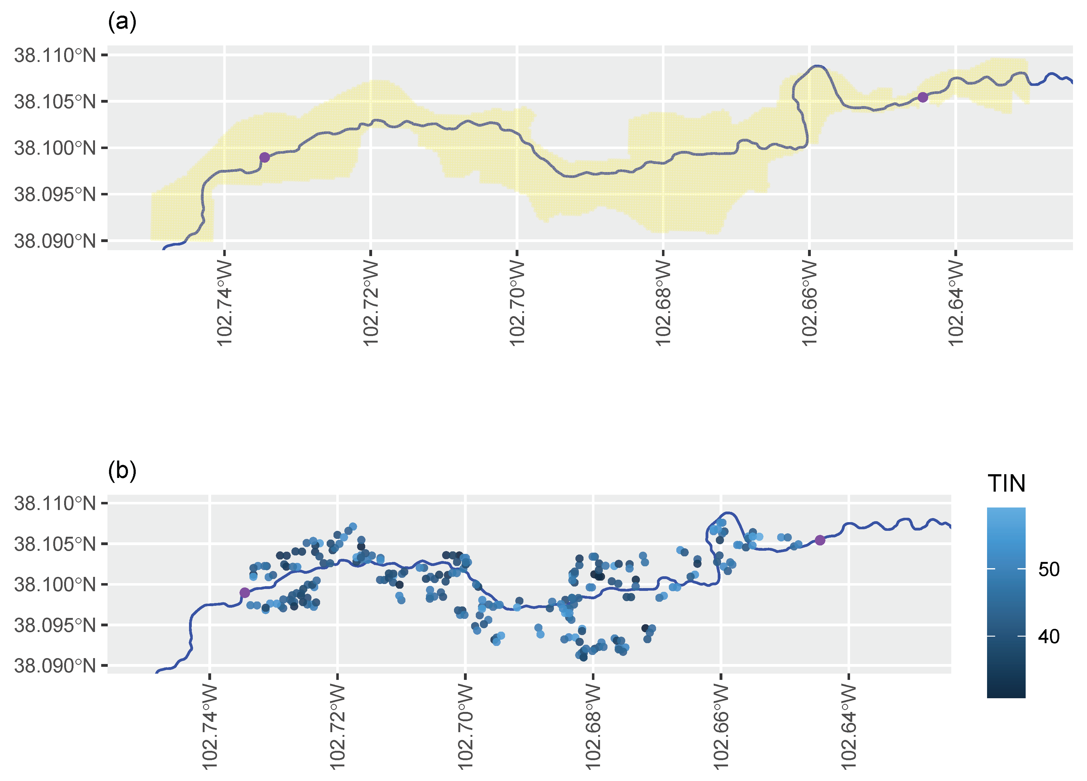
In order to represent ecosystem water use changes in a spatial format, temporal integration (i.e., sum) is applied to the average monthly NDVI to convert the time series into a single value of cumulative density at every Landsat pixel within the study region. The approach to integrated NDVI included herein is simpler than the methods proposed by Reed, Loveland, and Tiezen (1996), who defined the onset of greenness and summed all values of NDVI to a point in time when the plant is considered dormant [61]. The time period chosen to analyze temporally integrated NDVI is from January 2000 to December 2019. By 1996, several major surface-irrigation canals in the study area had been affected by augmentation [24], so January 2000 serves as an inflection point for land-use change. Satellite pixels are filtered in space and time to normalize each sub-region and thereby create an equal-area analysis among subregions (i.e., all subregions have the same number of observations of integrated NDVI per satellite pixel). The data filters are as follows: exclude data in space by removing all pixels with five or more observations of monthly NDVI less than 0, and exclude data in time by removing images with greater than 1% of missing areal data covering our study area. The filtered data are randomly sampled to create a data vector for the spatial analysis that is of size N d = 250 × 1 (0.225 km2) where N d is the number of spatial observations for each sub-region (See Appendix A Figure A1). The data are randomly sampled to reduce computational burden.

2.3. Temporal Covariates

Cumulative monthly precipitation (P), and average daily temperature per month (T) for the Upper Arkansas hydrologic boundary (HUC: 11020002) are downloaded from WestWide Drought Tracker [62]. Precipitation and temperature are assumed spatially uniform in the study area (i.e., all subregions share the same data), and these variables are standardized before being analyzed to reduce collinearity and improve model convergence [44].
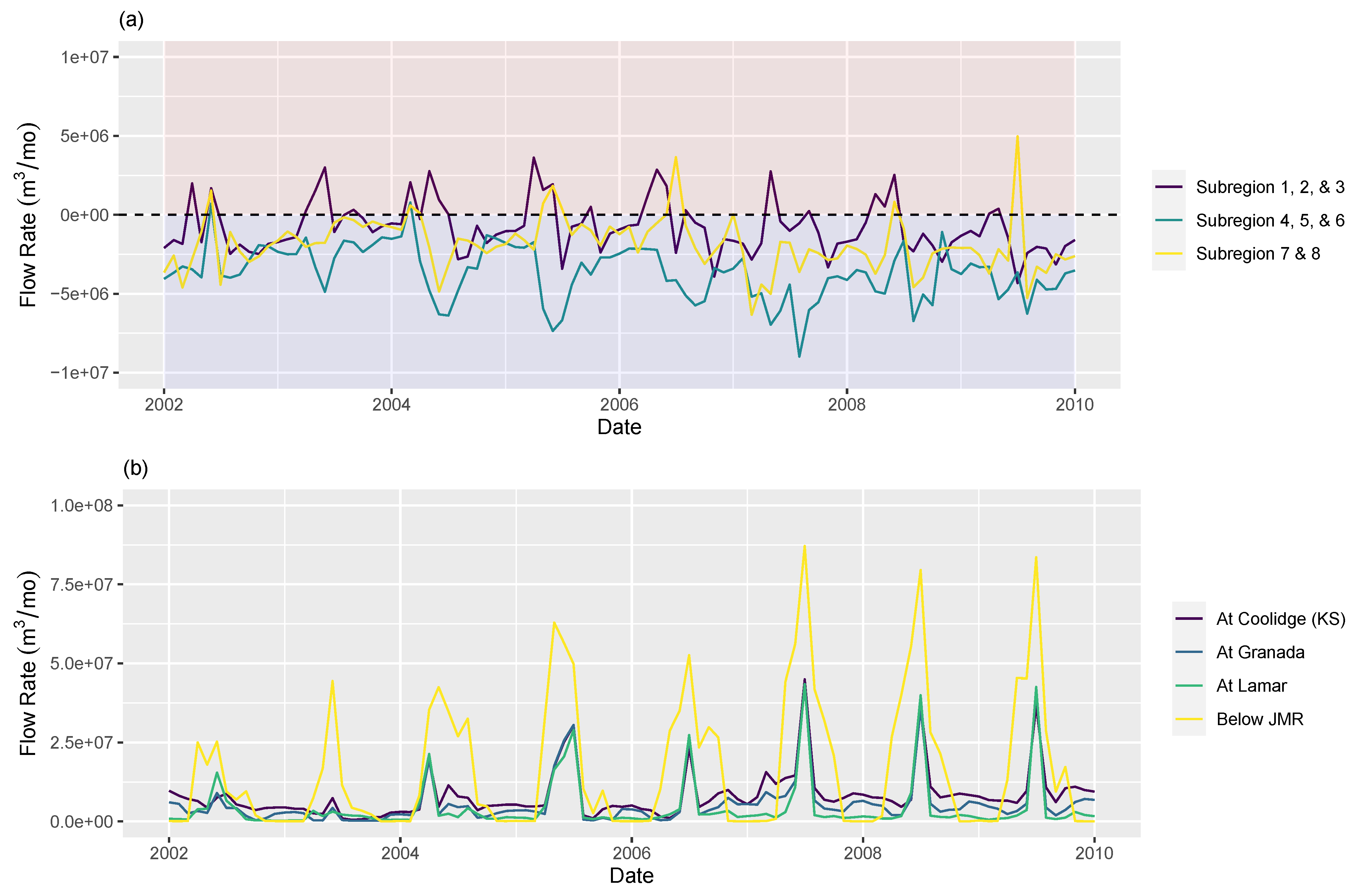
Monthly mean discharge for the Arkansas River is extracted from USGS Surface-Water Monthly Statistics for the Nation (U.S. Geological Survey, 2016) [52]. To create a surrogate variable for exchange flow, several USGS gages are used to perform a mass balance for each sub-region in the study area. This mass-balance technique converts discharge into a value of net stream gain or stream loss per month ( Q G / L t ), hereafter referred to as stream gain–loss. There are six USGS gages used in the stream gain–loss calculation with four on-stream gages and two tributary gages (Figure 1). The stream gain–loss covariate is used as the key proxy to connect the agro-ecosystem to the riparian ecosystem. The assumption is that when the river is gaining, then exchange flow (i.e., discharge from the alluvium to the river) is occurring. Figure 2 depicts the monthly discharge (using the nearest upstream gage) and monthly stream gain–loss applied to each subregion.
Data on monthly depth to groundwater (dtgw) are collected from the geographical information system hosted by Colorado’s Division of Water Resources [63]. There are numerous groundwater wells in the study area. One groundwater observation well is chosen for each sub-region based on the following criteria: duration of observations is from 1980 to 2018, and the observation well is within the spatial extent of the Quartenary Alluvium, shortest distance to the Arkansas River, and within the longitudinal extents of a subregion. The only exception to this criterion is the well used for sub-region 8, which is located at the downstream end of sub-region 7. This inconsistency is because sub-region 8 did not have observation wells that met the criteria above. Each observation record had to be extended to 2019 so the WestWide Drought Tracker [62] was used to find a similar hydrologic year, based on the percentage of normal precipitation, and the groundwater data from the hydrologically similar year replaced the missing data in 2019.

2.4. Spatial Covariates

Using Colorado’s Decision Support Systems Map Viewer, data for several landscape characteristics are compiled to explain spatial changes in temporally integrated riparian NDVI per subregion [63]. Each explanatory variable used in the spatial analysis is called a group, and each sub-region is assigned a value from each group. The groups are described in order as they appear in Table 2: (1) number of confluences, (2) are the operating canals outside of the riparian corridor impacted by augmentation [yes (1) or no (0)], (3) is there development (i.e., city or pastoral practices) located outside of the adjacent floodplain [yes (1) or no (0)], (4) is there a confluence between the Arkansas River and a perennial tributary [yes (1) or no (0)], and (5) is the sub-region adjoined by permanent dry up locations of irrigated land identified by the Substitute Water Supply Plans or decrees in Colorado for the Division of Water Resources [yes (1) or no (0)].
The spatial analysis includes count and binary variables that can be used to verify predictions about the connections between a riparian ecosystem and the surrounding landscape. The number of confluences is used as a count-covariate to account for the presence of drainage ditches, canals, and ephemeral draws in a sub-region as an indication for increased surface runoff and exchange flow (Group 1). Canal augmentation is coded as a binary covariate to track changing water availability in a sub-region as a result of altered soil-moisture and infiltration from modified irrigation methodologies (Group 2). Floodplain activity is a broad covariate that tests if pastoral practices and cities impact temporally integrated NDVI through altered surface runoff in timing and amount (Group 3). Confluence type is used as a binary covariate to account for the presence of a perennial tributary in a sub-region as an indication of a seasonally shallow groundwater table and increased exchange flow (Group 4). Irrigated land dry-up indicates subregions that are abutted by historic agricultural land that are no longer irrigated but can be re-irrigated with groundwater under a plan for augmentation, dryland-farmed, or have revegetation requirements (Group 5).

2.5. The Linear Models

The Bayesian multiple linear regression models used in the analyses are in Table 3. Model 1 is a classic linear regression model in a Bayesian setting that is used as the control model to validate the need to account for autocorrelation in our data. Model 2 is a hierarchical Bayesian linear time series model that accounts for an autoregressive signature of order one. Model 3 is a hierarchical Bayesian linear network model that accounts for spatial dependence among pixel neighbors within a given subregion. The reader is directed to Lurtz (2023) for a more in-depth understanding of the models used in this study [17]. A custom Markov chain Monte Carlo (MCMC) sampler is created for the models shown in Table 3 following the six general steps outlined by Hobbs and Hooten (2015) [44].
Model 2 equates to a fully Gibbs MCMC algorithm [17]. The model variables for the time series case are described as follows: y t comes from a univariate normal distribution and represents a measurement of monthly NDVI at time t = 1 , , T ; x t is a p × 1 vector of fixed covariates measured at time t where p represents the number of covariates; β is a multivariate normal p × 1 vector of regression coefficients with a p × 1 prior mean vector μ β and a p × p covariance matrix Σ β = σ β 2 I ; each I is an identity matrix with 1 on the diagonal elements of the matrix and 0 elsewhere; z t represents the autoregressive error in the ecohydrologic process at time t; and α is a scalar autocorrelation parameter of order one with hyperparameters μ α and σ α 2 . The data model variance, σ y 2 , accounts for the leftover variance not captured by the mean and autocorrelation components. The process model variance, σ z 2 , is a scalar that represents the variance in the autoregressive error, and z 0 is the initial state which comes from a univariate normal distribution.
The spatial model is a hybrid Gibbs and Metropolis–Hastings sampling scheme [17]. The spatial model is similar to the time series model in that the model accounts for a latent correlated process directly (i.e., z t in the temporal model and η d in the spatial model). The correlated process ( η d ) comes from a multivariate normal distribution; μ η d is the n d × 1 prior mean vector, and Σ ( σ η d 2 , ρ ) is an n d × n d covariance matrix set equal to σ η d 2 R ( ρ ) which is equivalent to σ η 2 ( diag ( W 1 d ) ρ W d ) 1 . diag ( W 1 d ) is a diagonal matrix with the row sums of W as diagonal elements [33]. This network model has W d as a binary distance matrix where locations within a certain distance of a pixel are neighbors [33]. In this study, the binary proximity matrix is developed for each sub-region by dictating that all pixels within 150 m of each other are considered neighbors (e.g., similar plant functional group). The spatial dependence parameter, ρ , is from a symmetric proposal with a univariate normal distribution set as the mean and a variance with a tuning parameter [33]. In the spatial formulation, σ d 2 represents the leftover variability after accounting for correlation among pixels that represent the same plant functional group. The variance in the spatially correlated random effect, σ η d 2 , is the expected error between the estimations of temporally integrated NDVI for image pixels that are neighbors and contain a similar plant functional group. The regression coefficients ( β ) and the spatial dependence parameter ( ρ ) are shared among subregions which forces smoothing across the eight subregions [50].

2.5.1. The Priors

The prior distributions represent insights about a variable in a statistical model and do not depend on the data being analyzed [44]. All variance structures are specified with strictly positive distributions (e.g., Gamma and IG). The autocorrelation coefficient in the time series model ( α ) is specified with a mean ( μ α ) equal to 0.6 and a variance ( σ α 2 ) equal to one because the correlation parameter is between −1 and 1 for stationary time series. The hyperparameters used to explain the covariance structures are vaguely specified with q z = 0.001 , r z = 1000 , q y = 0.001 , and r y = 1000 . The initial state variable has a mean of μ z 0 = 0 and a variance σ z 0 2 = 1 . The mean vector for the regression coefficients μ β is set equal to zero, and Σ β is equal to 10,000 I to control collinearity among covariates [33].
The priors in the spatial model are weakly informed similar to the time series approach, except for the spatial dependence parameter ( ρ ) and the spatially correlated effect ( η d ). The spatial dependence parameter has hyperparameters set to γ 1 = 9801 and γ 2 = 9900 , and ρ is instantiated in the MCMC chain close to one (e.g., 0.999) with a small tuning parameter ( ρ tune = 0.0005 ). The MCMC algorithm has an accept–reject sampling scheme so that the spatial dependence parameter remains between 0 and 1 [33]. The model is informed so that σ η d 2 comes from a mean of 5 and a variance of 4. This prior informing helps the model identify the spatial dependence among like vegetation communities as the smaller covariance between two covariance structures (e.g., σ d 2 and σ η d 2 ). The independent error variance, σ d 2 , is vaguely informed with q d = 0.001 and r d = 1000 .

2.5.2. Convergence, Model Checking, and Model Comparison

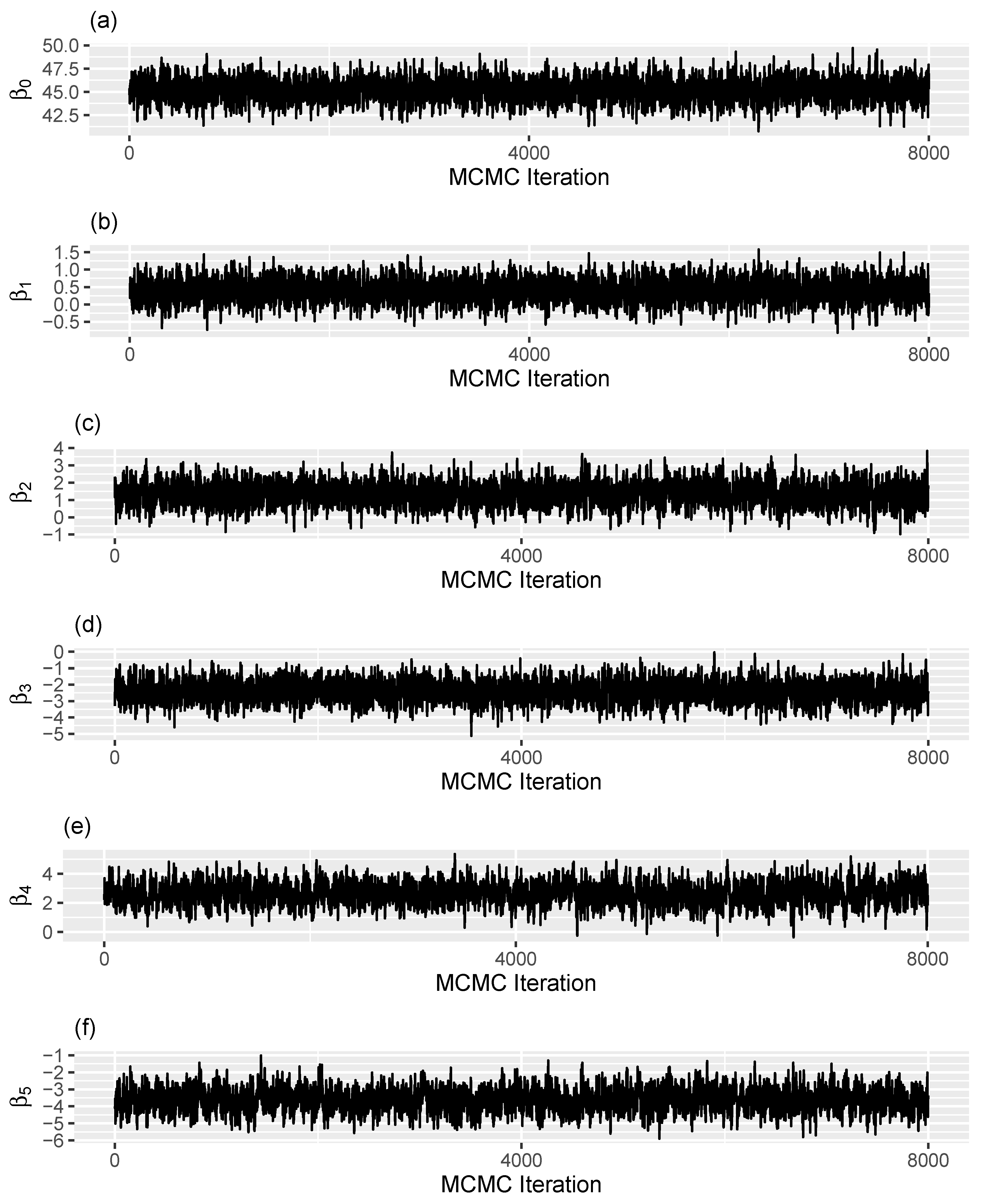
All models used in this analysis are checked for convergence by visual inspection of the MCMC trace plots (See examples in Appendix A Figure A2 and Figure A3). Posterior predictive distributions are used to determine if the models are capable of generating data that resemble the observed data [44]. The deviance information criterion (DIC) is used to measure how each covariate impacts the model in the time series approach. The DIC score is commonly used in Bayesian analysis and is good for comparing models of the same class [44]. The DIC is calculated as follows:
DIC = 2 log [ y | E ( θ | y ) ] + 2 p D
where the term −2log [ y | E ( θ | y ) ] represents the loss function, and 2 p D represents a penalty based on the number of model parameters [33]. The model with the lowest DIC score fits the data the best [33].

2.6. Prediction Testing

2.6.1. Hypothesis 1: Identifiable Temporal Trend at Catchment Scale

The temporal trend (growth or decay) is predicted to be identifiable at scales finer than catchment (10 km) because of first-hand experience with the vegetation distribution in the study area and previous research on the riparian trend [12,46]. To determine the spatial scale at which the temporal trend is identifiable, the study area is divided along the Arkansas River into successively smaller areas, and Model 2 is used to derive the correlation coefficient for the trend covariate. The baseline version of Model 2 consists of an intercept, trend, periodicity, an AR(1) component, and an independent error component (e.g., y t = α z t + β 0 + β 1 ( t ) + β 2 ( T t ) + ϵ t ). This study adopts definitions of scale in hydrology from Blöschl and Sivapalan (1995) [64]. The study area is divided into sub-areas with resolutions of large-reach scale (1 km), small-catchment scale (<5 km), catchment scale (>10 km), and sub-regional scale (100 km). If the 95% credible interval of the posterior distribution for β 1 does not overlap zero, this suggests there is growth or decay in time at a given spatial resolution.

2.6.2. Hypothesis 2: Precipitation Will Have a Shorter Lag Effect

Precipitation is assumed to have a shorter lag effect because the recent literature studying a riparian ecosystem with similar climatic conditions suggests that there are stronger relationships between riparian NDVI and precipitation compared to other hydrologic inputs like streamflow and reservoir stage [12,65,66]. We test this hypothesis by focusing on the intra-seasonal impacts of hydrologic and hydrosocial covariates (i.e., precipitation, discharge, exchange flow, and groundwater depth) on riparian NDVI using residual versus standardized predictor plots. Residuals are computed by fitting the baseline model (e.g., y t = α z t + β 0 + β 1 ( t ) + β 2 ( T t 2 ) + ϵ t ) to each NDVI time series to remove the autocorrelation, periodicity, and trend from each monthly NDVI time series to examine the leftover perturbations in NDVI as a function of lagged hydrologic and hydrosocial covariates (i.e., t, t 1 , and t 2 ). The DIC score confirmed that lagged monthly temperature ( t 2 ) was the best predictor to remove seasonality in the NDVI data.

2.6.3. Hypothesis 3: Confluences with Perennial Streams Increase Cumulative Vegetation Density

Perennial confluences with the Arkansas River are hypothesized to serve as a hydraulic boundary that uplifts the local groundwater table creating an exchange flow hotspot that supports existing and emerging vegetation. A spatial random effects model is used with a spatial partitioning approach, similar to one of many applied in Heaton et al. (2019) to test how floodplain characteristics impact riparian vegetation [50]. This regression model allows us to draw inferences about a variable relative to the other variables used in the model. We test this hypothesis by examining a form of derived distributions called contrasts [33]. The derived quantities are x ¯ a β , x ¯ b β , x ¯ c β , and x ¯ d β (where x ¯ a = ( 1 , x ¯ 2 , 1 , 0 , 0 , 0 ) , x ¯ b = ( 1 , x ¯ 2 , 0 , 1 , 0 , 0 ) , x ¯ c = ( 1 , x ¯ 2 , 0 , 0 , 1 , 0 ) ), and x ¯ d = ( 1 , x ¯ 2 , 0 , 0 , 0 , 1 ) ). These derived quantities are the average integrated NDVI for a riparian zone that is abutted by either augmentation or cities and pastoral practices or intersected by a perennial river or abutted by permanent irrigated land dry-up. The 95% credible intervals of the derived distributions are plotted to determine how perennial confluences impact cumulative vegetation density, relative to other variables tested in the model.

3. Results

3.1. Hypothesis 1: Identifiable Temporal Trend at Catchment Scale

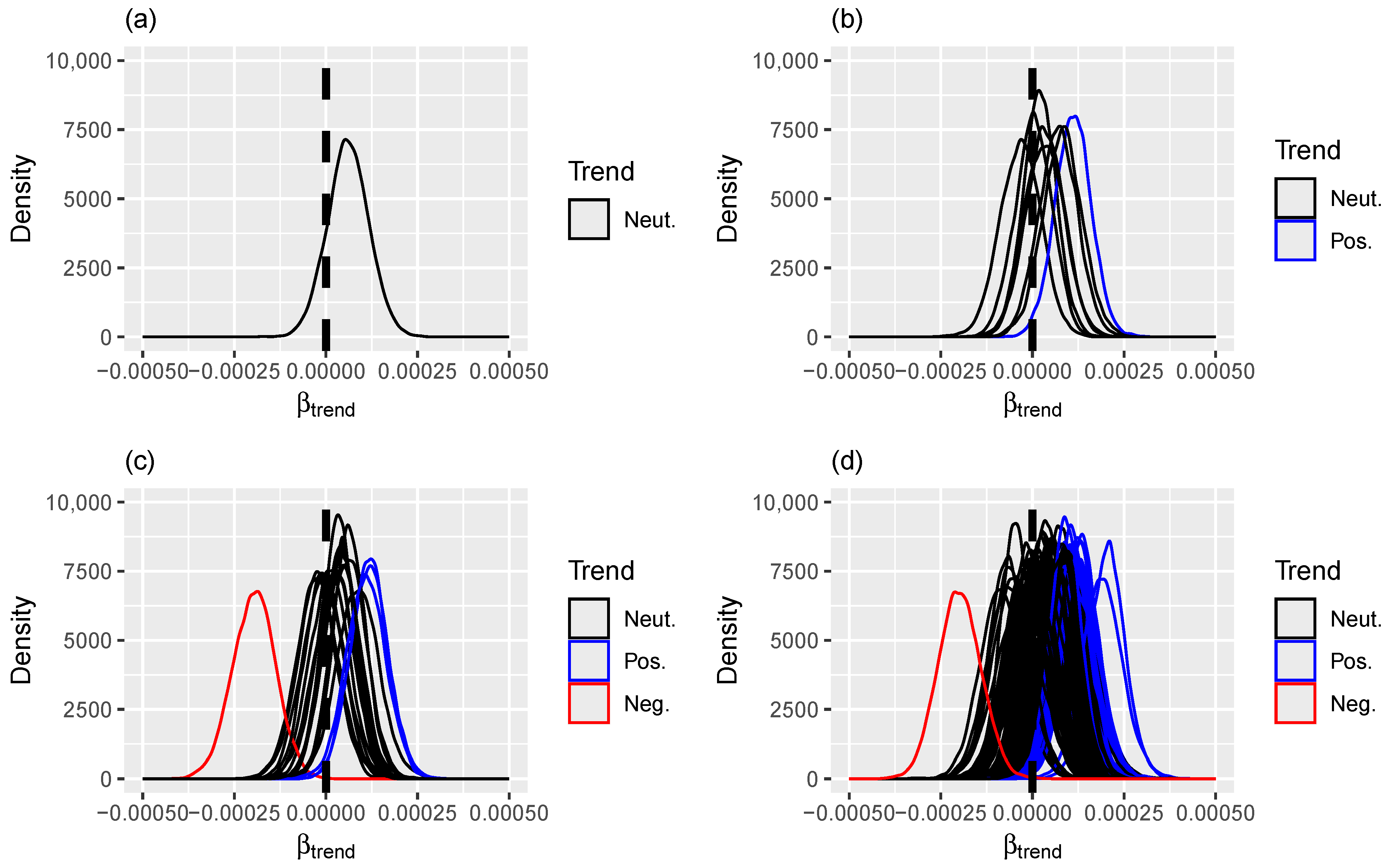
To address the first prediction, the study area is split into progressively finer scale riparian areas to determine the spatial-scale threshold for detecting a trend. The posterior distributions in Figure 3 corroborate the first hypothesis by indicating that a temporal trend, positive or negative, is not detectable at spatial scales coarser than catchment size (>10 km).
As summarized in Figure 3a, the correlation coefficient for the trend covariate overlaps zero (i.e., neutral trend) when the entire study area is examined using a single, areal average value of NDVI per month. Out of eight catchment-scale segments, the correlation coefficient for the trend covariate for sub-regionthree is positive, and the credible intervals do not overlap zero (Figure 3b). At spatial scales finer than catchment size, 4 of 19 (21%) segments of the Arkansas River have an identifiable trend (5 km scale), and 19 of 97 (20%) segments have an identifiable trend (1 km scale), growth or decay, from 1984 to 2019.

3.2. Hypothesis 2: Precipitation Will Have a Shorter Lag Effect

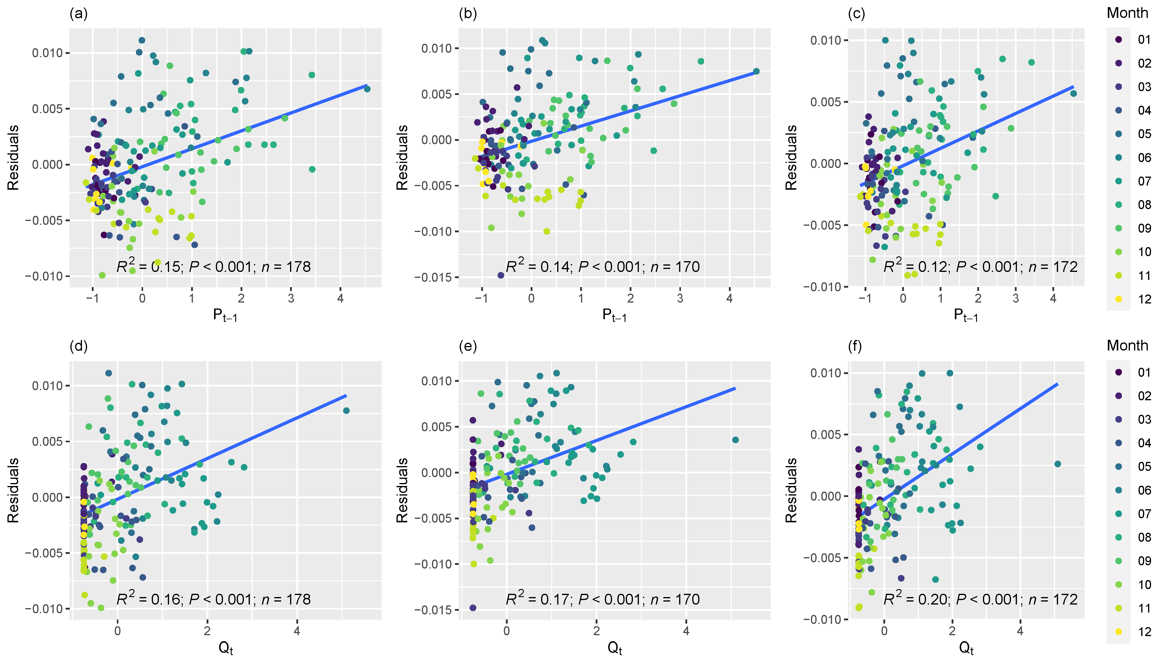
The second hypothesis is not supported by our analysis. Precipitation was mostly commonly correlated with model residuals at time t 1 across all sites except for sub-regioneight. Comparatively, river discharge showed slightly higher correlation with model residuals at time t which indicates, on a monthly time scale, river fluctuations correlate with riparian water use sooner in time than precipitation (Figure 4). All correlations between the residuals of the baseline model fit and explanatory covariates were low (i.e., R 2 < 0.4 ).
There are a variety of patterns between the residuals of the fitted model and the tested explanatory variables. While lagged precipitation showed consistent correlation to model residuals across subregions, discharge showed a decreasing pattern (i.e., R 2 decreased from t to t 2 ) of correlation at sub-region one, two, and three. Discharge showed the highest correlation at sub-region one, two, and three and no correlation at all other subregions. Stream gain–loss showed very poor to no correlation with model residuals at all subregions. Groundwater depth showed the highest correlations with model residuals at sub-region one ( R 2 = 0.28 at t 1 ), two ( R 2 = 0.29 at t 1 ), three ( R 2 = 0.31 at t 1 ), and eight ( R 2 = 0.34 at t 1 ).

3.3. Hypothesis 3: Confluences with Perennial Streams Increase Vegetation Density

The marginal posterior density plots for key spatial model parameters can be seen in Figure 5; this graph validates the third hypothesis. The mean and 95% central intervals (2.5% and 97.5%) for the contrasts can be seen in Figure 5. For the average sub-region investigated (e.g., average number of confluences), and with respect to all other model variables, areal segments that are intersected with perennial streams have larger temporally integrated NDVI. The contrast vector x ¯ c β indicates that subregions that have a perennial confluence have noticeable larger temporally integrated NDVI, while x ¯ b β (floodplain activity) and x ¯ d β (land dry-up) have a decreasing impact on temporally integrated NDVI.

4. Discussion

4.1. Hypothesis 1: Identifiable Temporal Trend at Catchment Scale

All subregions in the study area showed a strong first-order autoregressive signature. The relationship between the responses and covariates at time t and t 1 created the autoregressive structure, and the mean AR(1) value for all subregions combined was approximately 0.5. Temporal dependence in a water resource time series like the data analyzed in this study can be caused by atmospheric and hydrologic forcings, as well as agriculture and pastoral practices [38,67].
After accounting for the autoregressive component of each subregion’s time series, a temporal trend was identified in riparian NDVI at spatial resolutions finer than catchment scale (Figure 3). In terms of the strategic areas that were examined, the sub-region from the Amity canal to the Lamar gage was the only sub-region that showed a significant temporal trend in monthly NDVI as indicated by the posterior histogram that does not significantly overlap zero (95% credible interval), as summarized in Figure 3. Seven out of eight subregions did not exhibit a temporal trend in monthly NDVI at the operational scale. Figure 3a indicates a neutral trend at the sub-regional scale, but this result could be impacted by the section of the Arkansas River we examined (i.e., other sub-regional segments of the Arkansas River may show identifiable trends). In contrast, Nguyen et al. (2015) found a clear decreasing trend using linear least-squares analysis on mean annual values of riparian vegetation indices for a 39.51 km2 plot on the upper San Pedro River in Arizona [46]. The differences in the results between these two studies could be explained by differences in time series length (i.e., sample size), applied methodology, and the spatial scale at which the temporal trend is examined. For example, a negative trend is identifiable at spatial scales less than 5 km (Figure 3), although this could be due to landcover change (i.e, the conversion of agriculture land to fallow land).

4.2. Hypothesis 2: Precipitation Will Have a Shorter Lag Effect

The correlation of a two-month lag, or less, between precipitation and riparian NDVI is likely due to the area receiving most of its rainfall during the summer months and by spring snow replenishing soil moisture and recharging the aquifer in time for riparian green-up [24]. The lagged dependence between precipitation and riparian NDVI is consistent across all subregions, but this consistency could be due to the use of gridded precipitation compared to point-based data (i.e., precipitation could have local impacts not detected at the scale of analysis). Nguyen et al. (2015) found direct correlations between generalized NDVI and precipitation [46]. Vanderhoof et al. (2019) tested the significance of lagged precipitation to explain the temporal changes in riparian wetness and found that annual precipitation with drought indices are good predictors of the observed decline of riparian wetness [13]. Parsons and Thoms (2013) found discernible greenness changes in riparian vegetation during periods of increased rainfall and flooding [68]. Huntington et al. (2016) measured moderate but direct correlations between summer NDVI and annual precipitation and groundwater depth [14].
The residual versus standardized predictor plots reveal that discharge is correlated with riparian NDVI at the first three subregions downstream of the John Martin Reservoir (Figure 4). This result contrasts with findings on the San Pedro River in Arizona, USA, where remote sensing of ET showed perennial streams have higher correlation with atmospheric temperature than rainfall or stream discharge at the landscape scale [69]. The connection between reservoir-controlled discharge and riparian-NDVI response implies that connections between managed and natural ecosystems exist, and this evidence could be used to promote the use of environmental flows in the Arkansas River to improve natural ecosystem health. The variable Q G / L t is a proxy for exchange flow occurring between a stream segment and the alluvial aquifer. The lack of correlation between riparian NDVI and stream gain–loss is unexpected given the groundwater-dependent ecosystem being studied, and our mass balance indicates a gaining Arkansas River (Figure 2). Previous studies like Nagler et al. (2016) have used river discharge loss as a way to validate riparian water use for approximately 380 km2 of red gum riparian forests in the Yanga National Park, Australia [70]. Velpuri et al. (2020) used estimates of satellite-derived ET and river discharge to quantify how irrigation curtailment impacted the water balance in the upper Klamath Lake basin [71].
Most groundwater observations were recorded twice per year in the spring and fall to capture static water levels at pre- and post-irrigation time stamps. Groundwater depth had higher correlations with model residuals at time t 1 and t 2 , which indicates that changing groundwater depth has a delayed impact on riparian NDVI. While other studies have shown agreement between groundwater depth and NDVI [72,73], few studies have examined the delayed impact of groundwater depth on riparian water use.

4.3. Hypothesis 3: Confluences with Perennial Streams Increase Vegetation Density

Quantifying the connection of irrigating communities and riparian water use remains an elusive component of the hydrosocial framework. Spatial autoregressive statistics, like the model used here, are required when the data have spatial dependence and have been used to detect land use change from driving factors [74]. Based on the spatial analysis, a sub-region that has a confluence with a perennial stream (e.g., Mud, Big Sandy, and Wild Horse Creek) has increased integrated NDVI when compared to sites that are impacted by augmentation, floodplain activity, or permanent irrigated land dry-up (Figure 5). Albano et al. (2020) analyzed the residuals of a vegetation–climate regression analysis in relation to non-climatic forcings in Nevada and found, outside of the model, negative temporal trends in riparian vegetation were abutted by agriculture [12]. Albano et al. (2020) found growth in the temporal patterns of riparian vegetation that were connected to tributaries and perennial ponds and wetlands [12]. Vanderhoof et al. (2019), outside of the random forest regression, related the trend in the residuals of a climate–vegetation model fit to changing irrigation methodologies over a given area [13]. The spatial knowledge acquired from this work could be used to inform strategic field efforts aimed at preserving vulnerable ecosystems.

5. Conclusions

This work using statistical analysis on publicly available water resources data can be used to help resource managers understand lagged catchment processes in perturbed systems, but there are a few key drawbacks to this study to consider. We relied on the previous use of NDVI to measure groundwater-dependent ecosystems and did not investigate NDVI saturation [75]; however, semiarid GDEs typically include sparse vegetation. The spatial resolution of the Landsat NDVI product is coarse in that pixel-wide observations likely include more than one type of vegetation. The coarseness of the imagery makes inference on a specific vegetation type difficult in a heterogeneous riparian corridor. Future work on this subject could include imagery from new satellite platforms to overcome coarseness in time and space [76]. In the temporal and spatial analysis, the data model is Gaussian, which has support from to , and NDVI is strictly positive. This drawback is quickly overcome using conjugate relationships between the data, process, and parameters.
With the use of temporal and spatial statistics, this work provides an alternate way of validating previous observations and modeling that highlight floodplain connections to riparian ecosystems in groundwater-dependent regions. This work highlights that (a) temporal trend is spatial-scale-dependent (Figure 3), (b) gridded precipitation has a <2-month lagged correlation with riparian NDVI but varies upon sub-region (Figure 4) indicating an intra-seasonal dependence, and (c) perennial tributary confluences explain increased vegetation density (Figure 5). Future efforts in this direction may consider combining the independent analyses used in this investigation into a single spatio-temporal approach similar to Hooten and Wikle (2007) [77]. There is opportunity to link well-known models for handling spatial data with those for handling latent temporal patterns [78].

Author Contributions

Conceptualization, M.R.L. and R.R.M.; methodology, M.R.L.; formal analysis, M.R.L.; writing—original draft preparation, M.R.L., R.R.M. and P.L.N.; writing—review and editing, M.R.L., R.R.M. and P.L.N. All authors have read and agreed to the published version of the manuscript.

Funding

This work was originally funded by the Colorado Agricultural Experiment Station under Contract COL00756. Additional funding to continue and expand on this work was supported by a Graduate Teaching Fellowship in the Department of Civil Engineering at Colorado State University and by the National Science Foundation under Award No. 2305449. Any opinions, findings, and conclusions or recommendations expressed in this material are those of the author(s) and do not necessarily reflect the views of the National Science Foundation. Any use of trade, firm, or product name is for descriptive purposes only and does not imply endorsement by the U.S. Government.

Data Availability Statement

The datasets used in this study were derived from the following resources available in the public domain: Google Earth Engine [32], Colorado’s Division of Water Resources (https://dwr.colorado.gov/, accessed on 1 January 2023), and Surface-Water Monthly Statistics for the Nation United States Geological Survey (U.S. Geological Survey, 2016) [52]. The raw data and code supporting the conclusions of this article will be made available by the main author on request.

Acknowledgments

The authors would like to thank several representatives from Colorado’s Division of Water Resources in the Department of Natural Resources for guidance on data acquisition using the Decision Support Systems Map Viewer: Bill Tyner, Kelley Thompson, Monica Long, and Ivan Valles.

Conflicts of Interest

The authors declare no conflicts of interest. Pamela Nagler is an Associate Editor for the journal Remote Sensing. She is also the lead Guest Editor for the Special Issue on Monitoring Ecohydrology with Remote Sensing. She is not the handling editor for this submission. The funders had no role in the design of the study; in the collection, analyses, or interpretation of data; in the writing of the manuscript, or in the decision to publish the results.

Appendix A

Appendix A.1

Figure A1. Spatial representation of temporally integrated NDVI: (a) Location map for sub-region three with GDE delineation (transparent-yellow polygon), Arkansas River (blue line), and sub-region demarcations (purple points); (b) Location map for sub-region three with Arkansas River (blue line), sub-region demarcations (purple points) and 250 randomly sampled estimates of temporally integrated NDVI (TIN, blue points). Coordinate reference system: WGS84.
Remotesensing 16 02536 g0a1

Appendix A.2

Figure A2. Time series convergence summary plot for sub-region three in the form of Markov chain Monte-Carlo (MCMC) trace plots: (a) intercept ( β 0 ), (b) trend ( β 1 ), (c) temperature/seasonality ( β 2 ), (d) autogressive component ( α ), (e) data model variance ( σ y 2 ), and (f) process model variance ( σ z 2 ). MCMC iterations were 30,000 with 20% removed for the burn-in period.
Remotesensing 16 02536 g0a2
Figure A3. Convergence summary plot for the spatial analysis in the form of Markov chain Monte-Carlo (MCMC) trace plots: (a) intercept ( β 0 ), (b) number of confluences ( β 1 ), (c) canal augmentation ( β 2 ), (d) development ( β 3 ), (e) perennial tributary ( β 4 ), (f) land dry up ( β 5 ).
Remotesensing 16 02536 g0a3

References

  1. Saccò, M.; Mammola, S.; Altermatt, F.; Alther, R.; Bolpagni, R.; Brancelj, A.; Brankovits, D.; Fišer, C.; Gerovasileiou, V.; Griebler, C.; et al. Groundwater is a hidden global keystone ecosystem. Glob. Change Biol. 2023, 30, e17066. [Google Scholar] [CrossRef] [PubMed]
  2. Pace, G.; Gutiérrez-Cánovas, C.; Henriques, R.; Carvalho-Santos, C.; Cássio, F.; Pascoal, C. Remote sensing indicators to assess riparian vegetation and river ecosystem health. Ecol. Indic. 2022, 144, 109519. [Google Scholar] [CrossRef]
  3. Orellana, F.; Verma, P.; Loheide, S.P.; Daly, E. Monitoring and modeling water-vegetation interactions in groundwater-dependent ecosystems. Rev. Geophys. 2012, 3, 501–512. [Google Scholar] [CrossRef]
  4. Eamus, D.; Hatton, T.; Cook, P.; Colvin, C. Ecohydrology: Vegetation Function, Water and Resource Management; CSIRO Publishing: Clayton, VIC, Australia, 2006. [Google Scholar] [CrossRef]
  5. Kendy, E.; Bredehoeft, J.D. Transient effects of groundwater pumping and surface-water-irrigation returns on streamflow. Water Resour. Res. 2006, 8. [Google Scholar] [CrossRef]
  6. Ronayne, M.; Roudebush, J.; Stednick, J. Analysis of managed aquifer recharge for retiming streamflow in an alluvial river. J. Hydrol. 2017, 544, 373–382. [Google Scholar] [CrossRef]
  7. Bailey, R.T.; Wible, T.C.; Arabi, M.; Records, R.M.; Ditty, J. Assessing regional-scale spatio-temporal patterns of groundwater–surface water interactions using a coupled SWAT-MODFLOW model. Hydrol. Process. 2016, 23, 4420–4433. [Google Scholar] [CrossRef]
  8. Maddock, T.; Baird, K.; Hanson, R.; Schmid, W.; Ajami, H. RIP-ET: A riparian evapotranspiration package for MODFLOW-2005. U.S. Geol. Surv. Tech. Methods 2012, 6, A39. [Google Scholar]
  9. Loheide, S.P.; Gorelick, S. Riparian hydroecology: A coupled model of the observed interactions between groundwater flow and meadow vegetation patterning. Water Resour. Res. 2007, 43. [Google Scholar] [CrossRef]
  10. Tamea, S.; Laio, F.; Ridolfi, L.; D’Odorico, P.; Rodriguez-Iturbe, I. Ecohydrology of groundwater-dependent ecosystems: 2. Stochastic soil moisture dynamics. Water Resour. Res. 2009, 45. [Google Scholar] [CrossRef]
  11. Laio, F.; Tamea, S.; Ridolfi, L.; D’Odorico, P.; Rodriguez-Iturbe, I. Ecohydrology of groundwater-dependent ecosystems: 1. Stochastic water table dynamics. Water Resour. Res. 2009, 45. [Google Scholar] [CrossRef]
  12. Albano, C.; Mcgwire, K.; Hausner, M.; Mcevoy, D.; Morton, C.; Huntington, J. Drought Sensitivity and Trends of Riparian Vegetation Vigor in Nevada, USA (1985–2018). Remote Sens. 2020, 12, 1362. [Google Scholar] [CrossRef]
  13. Vanderhoof, M.; Christensen, J.; Alexander, L. Influence of multi-decadal land use, irrigation practices and climate on riparian corridors across the Upper Missouri River Headwaters Basin, Montana. Hydrol. Earth Syst. Sci. 2019, 23, 4269–4292. [Google Scholar] [CrossRef]
  14. Huntington, J.; McGwire, K.; Morton, C.; Snyder, K.; Peterson, S.; Erickson, T.; Niswonger, R.; Carroll, R.; Smith, G.; Allen, R. Assessing the role of climate and resource management on groundwater dependent ecosystem changes in arid environments with the Landsat archive. Remote Sens. Environ. 2016, 185, 186–197. [Google Scholar] [CrossRef]
  15. Groeneveld, D. Remotely-sensed groundwater evapotranspiration from alkali scrub affected by declining water table. J. Hydrol. 2008, 358, 294–303. [Google Scholar] [CrossRef]
  16. Tuinstra, J.; van Wensem, J. Ecosystem services in sustainable groundwater management. Sci. Total Environ. 2014, 485–486, 798–803. [Google Scholar] [CrossRef] [PubMed]
  17. Lurtz, M. Multiscale Connections between a Groundwater Dependent Ecosystem and Socio-Hydrology: Insight Gained from Numerical Modeling, Geospatial Informatics, and Bayesian Statistics. Ph.D. Thesis, Department of Civil and Environmental Engineering, Colorado State University, Fort Collins, CO, USA, 2023. [Google Scholar]
  18. Morway, E.D.; Gates, T.K.; Niswonger, R.G. Appraising options to reduce shallow groundwater tables and enhance flow conditions over regional scales in an irrigated alluvial aquifer system. J. Hydrol. 2013, 495, 216–237. [Google Scholar] [CrossRef]
  19. Scanlon, B.R.; Healy, R.W.; Cook, P.G. Choosing appropriate techniques for quantifying groundwater recharge. Hydrogeol. J. 2002, 10, 18–39. [Google Scholar] [CrossRef]
  20. Berghuijs, W.; Luijendijk, E.; Moeck, C.; van der Velde, Y.; Allen, S. Global Recharge Data Set Indicates Strengthened Groundwater Connection to Surface Fluxes. Geophys. Res. Lett. 2022, 49, e2022GL099010. [Google Scholar] [CrossRef]
  21. Gates, T.K.; Garcia, L.A.; Hemphill, R.A.; Morway, E.D.; Elhaddad, A. Irrigation Practices, Water Consumption, and Return Flows in Colorado’s Lower Arkansas River Basin: Field and Model Investigations; CWI Completion Report No. 221; CAES Report No. TR12-10; Colorado Water Institute: Fort Collins, CO, USA, 2012. [Google Scholar]
  22. Gates, T.K.; Steed, G.H.; Niemann, J.D.; Labadie, J.W. Data for Improved Water Management in Colorado’s Arkansas River Basin: Hydrological and Water Quality Studies; Colorado Water Institute Special Report No. 24; Colorado Agricultural Experiment Station No. TR-16-03; Colorado Water Institute: Fort Collins, CO, USA, 2016. [Google Scholar]
  23. Kittel, G.; Vanwie, E.; Damm, M.; Rondeau, R.; Kettler, S.; Mcmullen, A.; Sanderson, J. A Classification of Riparian Wetland Plant Associations of Colorado: User Guide to the Classification Project; Technical Report; Colorado Natural Heritage Program, Colorado State University: Fort Collins, CO, USA, 1999. [Google Scholar]
  24. Osborn, B. Lower Arkansas River Watershed Plan: John Martin Reservoir to Stateline; Technical Report; Colorado Water Institute—Colorado State University: Fort Collins, CO, USA, 2019. [Google Scholar]
  25. González-Sargas, E.; Shafroth, P.; Baró, F. Integrating social-ecological outcomes into invasive species management: The Tamarix case. NeoBiota 2024, 92, 173–192. [Google Scholar] [CrossRef]
  26. Hultine, K.R.; Froend, R.; Blasini, D.; Bush, S.E.; Karlinski, M.; Koepke, D.F. Hydraulic traits that buffer deep-rooted plants from changes in hydrology and climate. Hydrol. Process. 2020, 34, 209–222. [Google Scholar] [CrossRef]
  27. Yao, J.; Liu, H.; Huang, J.; Gao, Z.; Wang, G.; Li, D.; Yu, H.; Chen, X. Accelerated dryland expansion regulates future variability in dryland gross primary production. Nat. Commun. 2020, 20, 1665. [Google Scholar] [CrossRef] [PubMed]
  28. Nagler, P.; Morino, K.; Didan, K.; Erker, J.; Osterberg, J.; Hultine, K.; Glenn, E. Wide-area estimates of saltcedar (Tamarix spp.) evapotranspiration on the lower Colorado River measured by heat balance and remote sensing methods. Ecohydrology 2009, 2, 18–33. [Google Scholar] [CrossRef]
  29. Glenn, E.P.; Nagler, P.L.; Morino, K.; Hultine, K.R. Phreatophytes under stress: Transpiration and stomatal conductance of saltcedar (Tamarix spp.) in a high-salinity environment. Plant Soil 2013, 1–2, 655–672. [Google Scholar] [CrossRef]
  30. Yuana, G.; Zhang, P.; Shaoa, M.; Luoa, Y.; Zhu, X. Energy and water exchanges over a riparian Tamarix spp. stand in the lower Tarim River basin under a hyper-arid climate. Agric. For. Meteorol. 2014, 194, 144–154. [Google Scholar] [CrossRef]
  31. Brunke, M.; Gonser, T. The ecological significance of exchange processes between rivers and groundwater. Freshw. Biol. 1997, 37, 1–33. [Google Scholar] [CrossRef]
  32. Gorelick, N.; Hancher, M.; Dixon, M.; Ilyushchenko, S.; Thau, D.; Moore, R. Google Earth Engine: Planetary-scale geospatial analysis for everyone. Remote Sens. Environ. 2017, 202, 18–27. [Google Scholar] [CrossRef]
  33. Hooten, M.B.; Hefley, T.J. Bringing Bayesian Models to Life; Chapman and Hall/CRC: Boca Raton, FL, USA, 2019. [Google Scholar]
  34. Rumyantseva, O.; Sarantsev, A.; Strigul, N. Autoregressive Modeling of Forest Dynamics. Forests 2019, 10, 1074. [Google Scholar] [CrossRef]
  35. Jiang, B.; Liang, S.; Wang, J.; Xiao, Z. Modeling MODIS LAI time series using three statistical methods. Remote Sens. Environ. 2010, 14, 1432–1444. [Google Scholar] [CrossRef]
  36. Montanari, A.; Rosso, R.; Taqqu, M. Fractionally differenced ARIMA models applied to hydrologic time series: Identification, estimation, and simulation. Water Resour. Res. 1997, 33, 1035–1044. [Google Scholar] [CrossRef]
  37. Bras, R.L.; Rodriguez-Iturbe, I. Random Functions and Hydrology; Addison-Wesley Publ. Co.: Reading, MA, USA, 1985; ISBN 0-486-67626-9. [Google Scholar]
  38. Salas, J.D.; Tabios, G.Q., III; Bartolini, P. Approaches to multivariate modeling of water resources time series. J. Am. Water Resour. Assoc. 1985, 21, 683–708. [Google Scholar] [CrossRef]
  39. Shumway, R.H.; Stoffer, D.S. Time Series Analysis and Its Applications—With R Examples, 4th ed.; Springer: Cham, Switzerland, 2016. [Google Scholar]
  40. Fernandes, M.R.; Aguiar, F.C.; Ferreira, M.T. Assessing riparian vegetation structure and the influence of land use using landscape metrics and geostatistical tools. Landsc. Urban Plan. 2008, 99, 166–177. [Google Scholar] [CrossRef]
  41. Bastiaanssen, W.G.M.; Pelgrum, H.; Wang, J.; Ma, Y.; Moreno, J.F.; Roerink, G.J.; van der Wal, T. A remote sensing surface energy balance algorithm for land (SEBAL), Part 1: Formulation. J. Hydrol. 1998, 212–213, 198–212. [Google Scholar] [CrossRef]
  42. Elhaddad, A.; Garcia, L.A. Surface Energy Balance-Based Model for Estimating Evapotranspiration Taking into Account Spatial Variability in Weather. J. Irrig. Drain. Eng. 2008, 6, 681–689. [Google Scholar] [CrossRef]
  43. Senay, G.B.; Budde, M.; Verdin, J.P.; Melesse, A.M. A coupled remote sensing and simplified surface energy balance approach to estimate actual evapotranspiration from irrigated fields. Sensors 2007, 6, 979–1000. [Google Scholar] [CrossRef]
  44. Hobbs, N.T.; Hooten, M.B. Bayesian Models: A Statistical Primer for Ecologists; Princeton University Press: Princeton, NJ, USA, 2015. [Google Scholar]
  45. Anderson, K.; Fawcett, D.; Cugulliere, A.; Benford, S.; Jones, D.; Leng, R. Vegetation expansion in the subnival Hindu Kush Himalaya. Glob. Change Biol. 2019, 26, 1608–1625. [Google Scholar] [CrossRef]
  46. Nguyen, U.; Glenn, E.; Nagler, P.; Scott, R. Long-term decrease in satellite vegetation indices in response to environmental variables in an iconic desert riparian ecosystem: The Upper San Pedro, Arizona, United States. Ecohydrology 2015, 8, 610–625. [Google Scholar] [CrossRef]
  47. de Jong, R.; de Bruin, S.; de Wit, A.; Schaepman, M.E.; Dent, D.L. Analysis of monotonic greening and browning trends from global NDVI time-series. Remote Sens. Environ. 2010, 115, 692–702. [Google Scholar] [CrossRef]
  48. Lin, Y.; Xin, X.; Zhang, H.; Wang, X. The implications of serial correlation and time-lag effects for the impact study of climate change on vegetation dynamics—A case study with Hulunber meadow steppe, Inner Mongolia. Int. J. Remote Sens. 2015, 36, 5031–5044. [Google Scholar] [CrossRef]
  49. Hefley, T.; Broms, K.; Brost, B.; Buderman, F.; Kay, S.; Scharf, H.; Tipton, J.; Williams, P.; Hooten, M. The basis function approach for modeling autocorrelation in ecological data. Ecol. Concepts Synth. 2016, 98, 632–646. [Google Scholar] [CrossRef]
  50. Heaton, M.; Datta, A.; Finley, A.; Furrer, R.; Guinness, J.; Guhaniyogi, R.; Gerber, F.; Gramacy, R.; Hammerling, D.; Katzfuss, M.; et al. A Case Study Competition Among Methods for Analyzing Large Spatial Data. J. Agric. Biol. Environ. Stat. 2019, 24, 398–425. [Google Scholar] [CrossRef]
  51. Environmental Systems Research Institute. ArcGIS Desktop, v10.0+; Environmental Systems Research Institute: Redlands, CA, USA, 2011. [Google Scholar]
  52. U.S. Geological Survey. National Water Information System Data Available on the World Wide Web (USGS Water Data for the Nation). 2016. Available online: https://waterdata.usgs.gov/nwis (accessed on 1 January 2023).
  53. Senay, G.B.; Schauer, M.; Friedrichs, M.; Velpuri, N.M.; Singh, R.K. Satellite-based water use dynamics using historical Landsat data (1984–2014) in the southwestern United States. Remote Sens. Environ. 2017, 202, 98–112. [Google Scholar] [CrossRef]
  54. Hausner, M.; Huntington, J.; Nash, C.; Morton, C.; McEvoy, D.; Pilliod, D.; Hegewisch, K.; Daudert, B.; Abatzoglou, J.; Grant, G. Assessing the effectiveness of riparian restoration projects using Landsat and precipitation data from the cloud-computing application ClimateEngine.org. Ecol. Eng. 2018, 120, 432–440. [Google Scholar] [CrossRef]
  55. Eamus, D.; Zolfaghar, S.; Villalobos-Vega, R.; Cleverly, J.; Huete, A. Groundwater-dependent ecosystems: Recent insights from satellite and field-based studies. Hydrol. Earth Syst. Sci. 2015, 10, 4229–4256. [Google Scholar] [CrossRef]
  56. R Core Team. R: A Language and Environment for Statistical Computing; R Foundation for Statistical Computing: Vienna, Austria, 2023. [Google Scholar]
  57. Dewitz, J.; U.S. Geological Survey. National Land Cover Database (NLCD) 2019 Products; Earth Resources Observation and Science (EROS) Center: Sioux Falls, SD, USA, 2021.
  58. US Supreme Court Case 514, C. In AMENDED APPENDIX C.1, Hydrologic—Institutional Model: Model Documentation, Amended September 2011; Colorado Department of Water Resources: Denver, CO, USA, 2011.
  59. Ryan, J.A.; Ulrich, J.M.; Bennett, R.; Joy, C. xts: EXtensible Time Series. 2020. Available online: https://cran.r-project.org/web/packages/xts/index.html (accessed on 1 January 2023).
  60. Pettorelli, N.; Vik, J.; Mysterud, A.; Gaillard, J.; Tucker, C.; Stenseth, N. Using the satellite-derived NDVI to assess ecological responses to environmental change. Trends Ecol. Evol. 2005, 20, 503–510. [Google Scholar] [CrossRef] [PubMed]
  61. Reed, B.C.; Loveland, T.R.; Tiezen, L.L. An approach to using AVHRR data to monitor U.S. great plains grasslands. Geocarto Int. 1996, 11, 13–22. [Google Scholar] [CrossRef]
  62. Abatzoglou, J.T.; McEvoy, D.J.; Redmond, K.T. The West Wide Drought Tracker: Drought Monitoring at Fine Spatial Scales. Bull. Am. Meteorol. Soc. 2017, 98, 1815–1820. [Google Scholar] [CrossRef]
  63. Colorado Department of Natural Resources. Division of Water Resources. 2022. Available online: https://dwr.colorado.gov/ (accessed on 1 January 2023).
  64. Blöschl, G.; Sivapalan, M. Scale Issues In Hydrological Modelling: A Review. Hydrol. Process. 1995, 9, 251–290. [Google Scholar] [CrossRef]
  65. Scott, R.; Cable, W.; Huxman, T.; Nagler, P.; Hernandez, M.; Goodrich, D. Multiyear riparian evapotranspiration and groundwater use for a semiarid watershed. J. Arid Environ. 2008, 72, 1232–1246. [Google Scholar] [CrossRef]
  66. Nagler, P.; Glenn, E.; Kim, H.; Emmerich, W.; Scott, R.; Huxman, T.; Huete, A. Relationship between evapotranspiration and precipitation pulses in a semiarid rangeland estimated by moisture flux towers and MODIS vegetation indices. J. Arid Environ. 2007, 70, 443–462. [Google Scholar] [CrossRef]
  67. Bartolini, P.; Salas, J.; Obeysekera, J. Multivariate Periodic ARMA(1, 1) Processes. Water Resour. Res. 1988, 24, 1237–1246. [Google Scholar] [CrossRef]
  68. Parsons, M.; Thoms, M.C. Patterns of vegetation greenness during flood, rain and dry resource states in a large, unconfined floodplain landscape. J. Arid Environ. 2013, 88, 24–38. [Google Scholar] [CrossRef]
  69. Mayes, M.; Caylor, K.; Singer, M.; Stella, J.; Roberts, D.; Nagler, P. Climate sensitivity of water use by riparian woodlands at landscape scales. Hydrol. Process. 2020, 34, 4884–4903. [Google Scholar] [CrossRef]
  70. Nagler, P.; Doody, T.; Glenn, E.; Jarchow, C.; Barreto-Muñoz, A.; Didan, K. Wide-area estimates of evapotranspiration by red gum (Eucalyptus camaldulensis) and associated vegetation in the Murray-Darling River Basin, Australia. Hydrol. Process. 2016, 30, 1376–1387. [Google Scholar] [CrossRef]
  71. Velpuri, N.M.; Senay, G.B.; Schauer, M.C.; Garcia, A.; Singh, R.K.; Friedrichs, M.; Kagone, S.; Haynes, J.; Conlon, T. Evaluation of hydrologic impact of an irrigation curtailment program using Landsat satellite data. Hydrol. Process. 2020, 34, 1697–1713. [Google Scholar] [CrossRef]
  72. Lv, J.; Wang, X.; Zhou, Y.; Qian, K.; Wan, L.; Eamus, D.; Tao, Z. Groundwater-dependent distribution of vegetation in Hailiutu River catchment, a semi-arid region in China. Ecohydrology 2012, 1, 142–149. [Google Scholar] [CrossRef]
  73. Sims, N.; Colloff, M. Remote sensing of vegetation responses to flooding of a semi-arid floodplain: Implications for monitoring ecological effects of environmental flows. Ecol. Indic. 2012, 18, 387–391. [Google Scholar] [CrossRef]
  74. Overmars, K.P.; de Koning, G.H.J.; Veldkamp, A. Spatial autocorrelation in multi-scale land use models. Ecol. Model. 2003, 164, 257–270. [Google Scholar] [CrossRef]
  75. Huete, A.; Didan, K.; Miura, T.; Rodriguez, E.; Gao, X.; Ferreira, L. Overview of the radiometric and biophysical performance of the MODIS vegetation indices. Remote Sens. Environ. 2002, 83, 195–213. [Google Scholar] [CrossRef]
  76. McCabe, M.; Aragon, B.; Houborg, R.; Mascaro, J. CubeSats in Hydrology: Ultrahigh-Resolution Insights Into Vegetation Dynamics and Terrestrial Evaporation. Water Resour. Res. 2017, 53, 10017–10024. [Google Scholar] [CrossRef]
  77. Hooten, M.B.; Wikle, C.K. Shifts in the spatio-temporal growth dynamics of shortleaf pine. Environ. Ecol. Stat. 2007, 14, 207–227. [Google Scholar] [CrossRef]
  78. Comber, A.; Wulder, M. Considering spatiotemporal processes in big data analysis: Insights from remote sensing of land cover and land use. Trans. GIS 2019, 23, 879–891. [Google Scholar] [CrossRef]
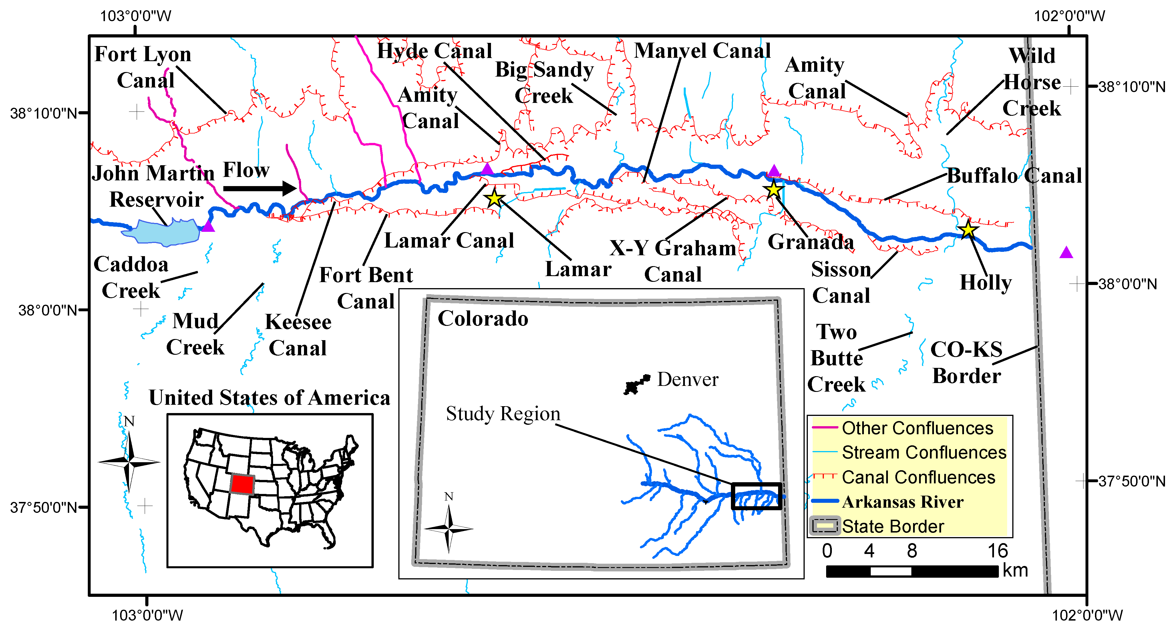
Figure 1. General location map of the 96 km reach of the Arkansas River located downstream of the John Martin Reservoir (JMR). Yellow stars indicate a township or city. Purple triangles represent four of six U.S. Geological Survey (USGS) gages located on the Arkansas River: Below JMR (ID: 07130500; 38.07°, −102.93°), at Lamar, CO (ID: 07133000; 38.11°, −102.62°), near Granada, CO (ID: 07134180; 38.10°, −102.31°), near Coolidge, KS (ID: 07137500; 38.03°, −102.01°) [51]. Two gages, not shown for simplicity, used in the time series analysis are Big Sandy Creek near Lamar, CO (ID: 07134100; 38.11°, −102.48°) and Wild Horse Creek above Holly, CO (ID: 07134990; 38.06°, −102.14°) (U.S. Geological Survey, 2016) [52].
Remotesensing 16 02536 g001
Figure 2. (a) Time series of monthly stream gain–loss from 1 January 2002 to 1 January 2010; negative values of stream gain–loss indicate a net gain (transparent blue) to the Arkansas River, and positive values indicate a net loss (transparent red). The dashed black line demarcates the point at which no exchange flow occurs. (b) Time series of monthly discharge from 1 January 2002 to 1 January 2010 for the four USGS gages located on the main stem of the Arkansas River.
Remotesensing 16 02536 g002
Figure 3. Marginal posterior densities for β t r e n d estimated at varying spatial resolutions: (a) sub-regional scale (100 km); (b) catchment scale or operational scale based on subregions (>10 km); (c) small-catchment scale (<5 km); (d) large-reach scale (1 km).
Remotesensing 16 02536 g003
Figure 4. Residual versus standardized predictor plots: (a,d) Sub-region one comparisons with precipitation at t 1 and discharge at time t; (b,e) Sub-region two comparisons with precipitation at t 1 and discharge at time t; (c,f) Sub-region three comparisons with precipitation at t 1 and discharge at time t.
Remotesensing 16 02536 g004
Figure 5. Derived distributions in the form of contrasts. The yellow circles represent the mean, and the purple vertical lines represent the span of the 95% credible interval for each derived distribution. The dashed black line represents the mean integrated NDVI value for a sub-region not impacted by any of the floodplain characteristics analyzed in this study.
Remotesensing 16 02536 g005
Table 1. A summary of the sub-region demarcations that correspond to the Hydrologic Institutional Model to simulate water processes on the Arkansas River. The Δ Dist. (km) is the incremental length of each river segment in a subregion.
No.NameLocation (Long.°) Δ Dist. (km)
1Below JMR to Below Fort Bent Canal(begin, −102.8°]10.03
2Below Fort Bent Canal to Below Amity Canal(−102.8°, −102.7°]11.38
3Below Amity Canal to Lamar Gage(−102.7°, −102.6°]10.48
4Lamar Gage to Below Manvel Canal(−102.6°, −102.5°]17.39
5Below Manvel Canal to Below X-Y Graham Canal(−102.5°, −102.4°]8.78
6Below X-Y Graham Canal to Granada Gage(−102.4°, −102.3°]11.28
7Granada Gage to Below Sisson-Stubbs Canal(−102.3°, −102.2°]14.43
8Below Sisson-Stubbs Canal to CO-KS Border(−102.2°, end]12.80
Table 2. A summary of the subregions with count and binary variables incorporated into a coding matrix.
-Group 1Group 2Group 3Group 4Group 5
SubregionNo. of ConfluencesCanal AugmentationDevelopmentPerennial TributaryLand Dry-Up
140000
231011
321100
420100
511011
621000
720001
831010
Table 3. A summary of the models used in this study. The symbol ∼ implies two sides of an equation are proportional to each other. The probability distribution abbreviations are as follows: Normal-Gaussian (N), multivariate normal (MVN), and Inverse Gamma (IG).
Model 1 (General)Model 2 (Time)Model 3 (Space)
y i N ( x i β , σ 2 ) y t N ( x t β + z t , σ y 2 ) y d MVN ( X d β + η d , σ d 2 I )
β MVN ( μ β , Σ β ) z t N ( α z t 1 , σ z 2 ) η d MVN ( μ η , Σ ( σ η d 2 , ρ ) )
σ 2 IG ( q , r ) β MVN ( μ β , Σ β ) β MVN ( μ β , Σ β )
α N ( μ α , σ α 2 ) ρ Gamma ( γ 1 , γ 2 )
σ y 2 IG ( q y , r y ) σ d 2 IG ( q d , r d )
σ z 2 IG ( q z , r z ) σ η d 2 IG ( q η , r η )
z 0 N ( μ z 0 , σ z 0 2 )
Disclaimer/Publisher’s Note: The statements, opinions and data contained in all publications are solely those of the individual author(s) and contributor(s) and not of MDPI and/or the editor(s). MDPI and/or the editor(s) disclaim responsibility for any injury to people or property resulting from any ideas, methods, instructions or products referred to in the content.