Article

A Target Detection Algorithm Based on Fusing Radar with a Camera in the Presence of a Fluctuating Signal Intensity

School of Information and Communication Engineering, Hainan University, Haikou 570228, China
*
Author to whom correspondence should be addressed.
Remote Sens. 2024, 16(18), 3356; https://doi.org/10.3390/rs16183356
Submission received: 29 July 2024 / Revised: 2 September 2024 / Accepted: 4 September 2024 / Published: 10 September 2024
(This article belongs to the Special Issue Technical Developments in Radar—Processing and Application)

Abstract

:
Radar point clouds will experience variations in density, which may cause incorrect alerts during clustering. In turn, it will diminish the precision of the decision-level fusion method. To address this problem, a target detection algorithm based on fusing radar with a camera in the presence of a fluctuating signal intensity is proposed in this paper. It introduces a snow ablation optimizer (SAO) for solving the optimal parameters of the density-based spatial clustering of applications with noise (DBSCAN). Subsequently, the enhanced DBSCAN clusters radar point clouds, and the valid clusters are fused with monocular camera targets. The experimental results indicate that the suggested fusion method can attain a Balance-score ranging from 0.97 to 0.99, performing outstandingly in preventing missed detections and false alarms. Additionally, the fluctuation range of the Balance-score is within 0.02, indicating the algorithm has an excellent robustness.

1. Introduction

With vehicle ownership increasing, traffic safety and congestion problems have become increasingly severe. According to the statistical analysis, traffic accidents caused by humans, such as distraction and fatigue driving, are as high as 94% [1,2]. In this context, developing intelligent driving vehicles that aim to reduce traffic accidents has become a research hotspot [3,4]. The intelligent driving system mainly uses sensors such as LiDAR, cameras, and radar to sense information about targets [5,6]. Where LiDAR offers benefits such as high detection precision and an extensive detection range, but it is susceptible to weather and difficult to obtain the texture features of targets [7]. Although cameras are sensitive to target textures [8,9,10,11], they usually suffer from drawbacks such as large-ranging errors and susceptibility to weather [12,13]. On the contrary, radar can not only provide precise information about distance and speed, but can also work well around the clock [14,15,16,17]. However, it is difficult for radar to acquire the attributes of the targets [18].
In summary, each type of sensor has drawbacks, making it challenging to meet the requirements of complex environments. Therefore, using multi-sensor fusion methods to sense targets has become a trend in intelligent driving. Information fusion techniques can fully utilize the benefits of various sensors, thus enhancing redundancy and stability in the recognition system [19]. Currently, the radar-vision (RV) fusion method has become mainstream due to its ability to achieve a high detection accuracy with minimal computational and cost sacrifices [20,21].
The RV fusion methods are divided into data level, feature level, and decision level [22]. Where the decision-level fusion strategy first processes the data detected by different sensors individually, and then compares, evaluates, and correlates the processing results [23]. Because the structure and idea of this strategy are simple, it has become mainstream. However, its performance is usually limited by specific combinations of sensors and algorithms. For example, if radar false alarms are frequent, the accuracy of the fusion algorithm will dramatically decrease.
In [24], the authors utilize the constant false-alarm rate (CFAR) to process the radar data so as to reduce noise and false alarms. However, the method’s performance will drop drastically when the strength of the noise or interfering signal is strong. To solve this problem, ref. [25] plotted targets detected by radar on the image, and applied a Gaussian Mixture Model (GMM) to segment the dynamic targets from the static background. However, the method will be limited by the coordinate transformation error. In [26], the authors filtered out the background objects, such as road signs and bins, by setting a speed threshold. Nevertheless, because this method compares the velocity of all objects detected by radar to the same threshold, it is prone to situations where the valid targets will be misclassified as disturbances. For solving this problem, ref. [27] processed the radar point clouds using the density-based spatial clustering of applications with noise (DBSCAN), which can separate targets with a different reflectivity. Then, the valid objects from the radar and camera were fused. Nonetheless, DBSCAN requires pre-setting parameters, which will limit its generalizability and accuracy [28].
To summarize, the results of existing decision-level fusion methods usually depend on the specific combination of algorithms for sensors. In particular, when the echo signal strengths of the targets to be detected are diverse, the radar’s false alarms will increase dramatically. Accompanying, the effectiveness of fusion will decrease. To tackle this issue, a target detection algorithm based on fusing radar with a camera in the presence of a fluctuating signal intensity is proposed in this paper. Firstly, it introduces the snow ablation optimizer (SAO) [29] for solving the optimal parameters of DBSCAN. And the enhanced DBSCAN, which we name SAO-DBSCAN, is applied for clustering radar point clouds. Then, the targets in the image are extracted using the YOLOv5s model [30]. Finally, targets identified by radar and camera are integrated through a decision-level fusion strategy. Experiments indicate that the suggested fusion method can achieve excellent accuracy and be applied to scenarios where the intensities of the echo signal vary. This research makes several contributions, which are outlined below:
(1) We introduce the SAO to optimize the parameters of DBSCAN. This method does not require manual parameter adjustment and has excellent generality.
(2) We use the proposed SAO-DBSCAN to cluster the radar point clouds, which can automatically determine the optimal parameters based on the distribution of the point clouds, thereby significantly decreasing the radar false alarms.
(3) We fuse the valid clusters, which are obtained by the proposed SAO-DBSCAN, with the objects detected by a camera. It can enhance the precision of the decision-level fusion method by reducing false alarms from radar.
The remainder of the paper is structured as follows: Section 2 exhibits the fusion model. Section 3 describes some critical steps and algorithms of fusion. In Section 4, we showcase and analyze the experimental findings. Finally, Section 5 summarizes the conclusions.

2. Information Fusion Model

For the fusion model suggested in this study, radar primarily delivers the targets’ positions and velocities, while the camera supplies their classifications. In addition, the camera is also responsible for acquiring the lane information, which helps fuse video data with radar from a same lane line. The schematic is illustrated in Figure 1.
For the decision-level fusion strategy, it is crucial to process the data detected by each sensor separately before fusion. In the vision-based target detection module, we first use a second-order polynomial to extract the lane information in the picture [31]. Then, the YOLOv5s model is employed to identify the objects on the image. In the radar-based target detection module, data from radar are first pre-processed. Then, the radar point clouds reflected from each target are clustered by the proposed SAO-DBSCAN. Subsequently, we utilize the lane lines to eliminate interferences that lie outside the lanes, and mark the lane information of the valid objects that remain [32].
In the fusion-based target detection model, data detected by the two sensors are temporally aligned through software. And the spatial alignment is achieved based on the positional relationship between the two sensors. Next, we calculate the intersection over union (IOU) based on the detection boxes between objects identified by different sensors in the same lane. Finally, the value of IOU is used to achieve target-matching between sensors for information fusion.

3. Realization of Fusion

3.1. Radar Data Processing

3.1.1. Signal Model of the FMCW Radar

Here, the frequency-modulated continuous wave (FMCW) radar has been utilized to gather information about targets. Its basic principle is constructing an intermediate frequency (IF) signal using the transmitted and echo signals [33]. Assuming that the sampling period is T s , the expression for the IF signal is as follows:
S IF ( m , l , n ) = e j 4 π f 0 R e j 2 π dsin θ λ m e j 2 π 2 f 0 v c l e j 2 π f 0 2 v c + B 2 R T c nT s
where S IF ( m , l , n ) denotes the sample at the m−th antenna, the l−th frequency-modulation (FM) cycle, and the n−th sampling moment. T c is the duration of an FM cycle. f 0 represents the starting frequency of the transmitted signal. c indicates the velocity of light. d indicates the separation of neighboring array elements whose value is d = 2 π f 0 / c . Additionally, θ , R , and v represent the azimuth, distance, and velocity, respectively, between the target and radar. After pre-processing the IF signal, we can generate the radar point clouds for clustering.

3.1.2. The Improved DBSCAN Algorithm

DBSCAN [34] is a clustering algorithm based on density that focuses on grouping regions with varying densities into separate clusters. It is composed of two concepts: ε and MinPts . Where ε represents the domain radius of the sample points, and MinPts signifies the minimum quantity of point clouds within each cluster. Based on the above concepts, the samples can be divided into core, border, and noise points by DBSCAN, as shown in Figure 2.
The core point indicates that the quantity of points contained in its ε - neighborhood is at least MinPts. The border points are characterized by having fewer samples than MinPts in their ε - neighborhood , but they are located within the core point’s ε - neighborhood . The noise points are those except the core and border points. The basic modeling steps for DBSCAN are shown below:
(1) Choose any sample X i in the dataset as a point P in the space.
(2) Search for samples in the ε - neighborhood of point P . If the number of samples exceeds or is equal to MinPts, all points within the ε - neighborhood of P belong to the same cluster.
(3) Repeat Step (2) starting from the neighboring samples of point P until all samples in the dataset have been traversed. Ultimately, clusters that represent targets and noise are obtained.
The advantages of DBSCAN are that it can recognize noise in radar point clouds, as well as handle clusters with different shapes and sizes. However, its generalizability is poor. This is because the parameters of DBSCAN have to be pre-set, which makes it challenging to utilize in situations with significant fluctuations in point cloud density. To adaptively solve the optimal parameters according to the density of the point clouds, we introduce the SAO algorithm to improve DBSCAN. The methodology mainly consists of three phases: initialization, exploration, and exploitation. Additionally, a dual population scheme is utilized to balance the exploration and exploitation. Its basic principles are as follows:
Fistly, we define the optimization function ( fitness ) of SAO as follows:
fitness = 1 S
where S , taking the value in the range of [ 1 , 1 ] , is called the average silhouette coefficient [35] of clustering. And, as the value of S increases, the clustering performance will improve. Assuming that the point clouds are divided into C clusters by DBSCAN, the formula for S is as follows:
S = 1 C i = 1 C S ( p i )
S ( p i ) = b ( p i ) a ( p i ) max { b ( p i ) , a ( p i ) }
where S ( p i ) denotes the silhouette coefficient of each cluster. The role of a ( p i ) is to quantify the cohesion within the cluster. Its value is derived from the average of the distances between p i and other samples in its ε - neighborhood . b ( p i ) denotes the smallest value of the mean distances from p i to all points in the neighboring clusters, which is used to quantify the separation among clusters.
During the initialization phase, the upper (U) and lower (L) limits of the parameters to be optimized are pre-set. Then, the snow cluster J is generated:
J = L + β × ( U L )
where β is a random number with a value in the range of [0,1]. As the parameters of DBSCAN are ε and MinPts, J can be written as follows:
J = ε 1 MinPts 1 ε 2 MinPts 2 ε K MinPts K
where K denotes the size of the snow cluster.
During the exploration phase, a probability density function of the standard normal distribution is used to model the highly dispersive Brownian Motion phenomenon [36], which occurs when the snow-melted water is transformed into steam. Its mathematical expression is as follows:
f BM ( x ) = 1 2 π e x 2 / 2 .
Therefore, the positional update formula for this phase is as follows:
J ( j , t + 1 ) = J elite ( t ) + p BM ( j , t ) ( β 1 × ( J 1 st ( t ) J ( j , t ) ) + ( 1 β 1 ) × ( J ¯ ( t ) J ( j , t ) ) )
where ⊗ denotes entry-wise multiplications. β 1 denotes a random number from 0 to 1. p BM ( j , t ) is a random vector generated with a Gaussian distribution, which is used to represent the phenomenon of Brownian Motion. J ( j , t ) denotes the particle j in the snow cluster during iteration t. J 1 st ( t ) represents the current optimal particle. J ¯ ( t ) denotes the mean value of the whole snow cluster. And J elite ( t ) is an elite set. The mathematical expressions for J ¯ ( t ) and J elite ( t ) are as follows:
J ¯ ( t ) = 1 K j = 1 K J ( j , t )
J elite ( t ) = [ J 1 st ( t ) , J 2 nd ( t ) , J 3 rd ( t ) , J 1 / 2 ( t ) ]
where J 2 nd ( t ) is the second-best particle and J 3 rd ( t ) is the third-best. J 1 / 2 ( t ) is the mean value of the snow cluster ranked in the top 50 percent of fitness values:
J 1 / 2 ( t ) = 1 K 1 j = 1 K 1 J ( j , t ) .
Here, the value of K 1 is taken to be half of K .
During the exploitation phase, the snow-melt model mainly develops around the current optimal solution rather than further extending its high dispersion. The positional update formula for this phase is as follows:
J ( j , t + 1 ) = S M ( t ) × J 1 st ( t ) + p BM ( j , t ) ( β 2 × ( J 1 st ( t ) J ( j , t ) ) + ( 1 β 2 ) × ( J ¯ ( t ) J ( j , t ) ) )
where β 2 denotes a random number that takes a value in the range of [ 1 , 1 ] . And S M ( t ) is the snow-melt rate, which is expressed as follows:
S M ( t ) = ( 0.35 + 0.25 × e t t max 1 e 1 ) × e t t max
where t max denotes the maximum number of iterations.
Finally, the SAO algorithm designs a dual population scheme. It aims at balancing the exploration and exploitation phases. At the early stage of the optimization search, this scheme randomly divides the entire snow cluster into two equal-sized sub-populations, which are responsible for exploration and exploitation. As the iteration progresses, the membership of sub-population 1 dedicated to exploration gradually decreases. At the same time, the membership of sub-population 2 dedicated to exploitation gradually increases. Figure 3 illustrates the block diagram of the suggested SAO-DBSCAN.

3.2. Video Data Processing

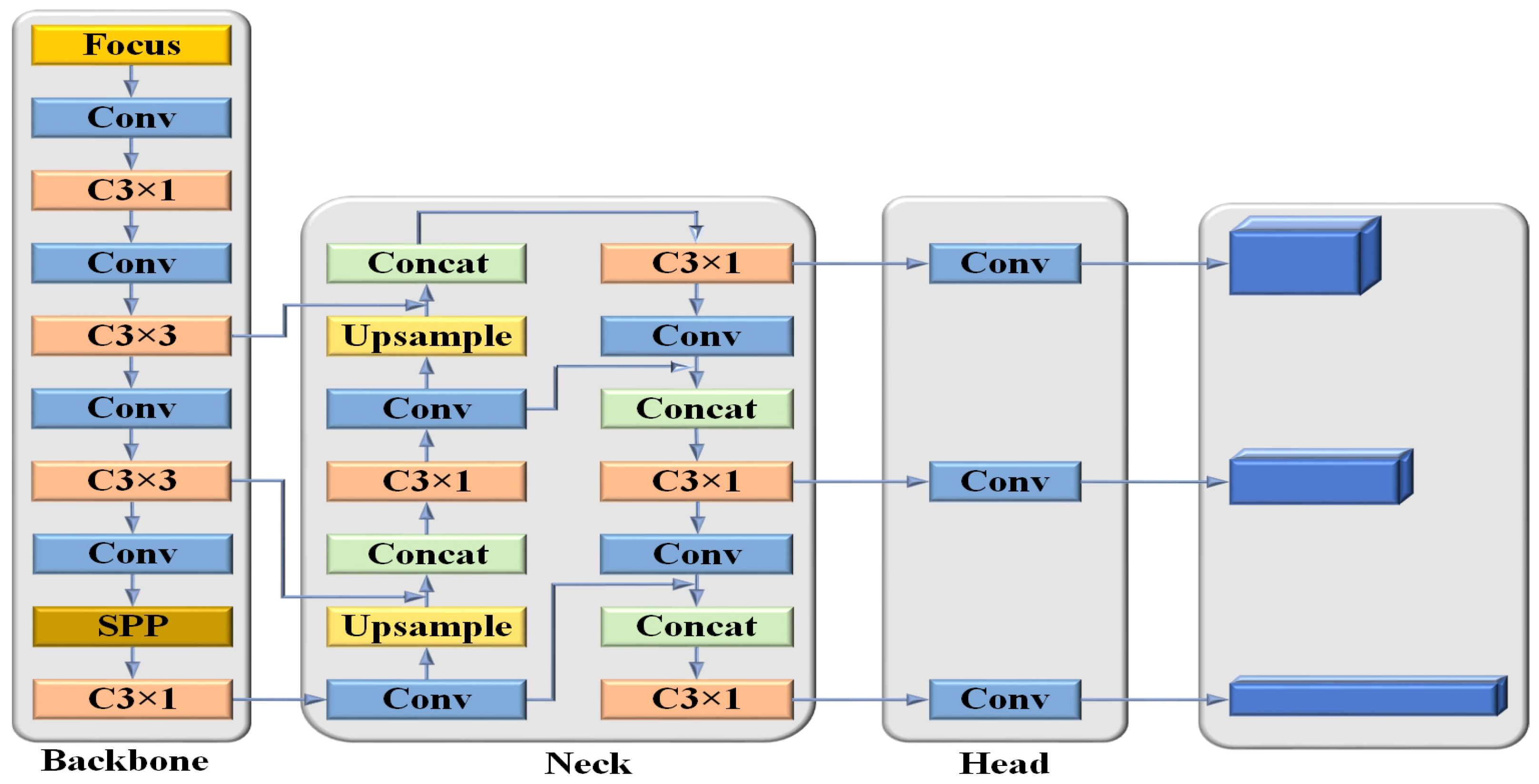
In this study, the YOLOv5s model is used to extract the targets in the image. Its structure is shown in Figure 4. This model mainly consists of the feature extraction network (Backbone), the feature fusion network (Neck), and the detection head (Head) [37,38]. Where the Backbone network is used to extract the targets’ features. The Neck network is used to fuse the features of different scales. The Head network is used to perform classification, regression, and prediction. It contains three detection heads, which are used to detect large, medium, and small targets.

3.3. Spatio-Temporal Calibration

3.3.1. Temporal Alignment

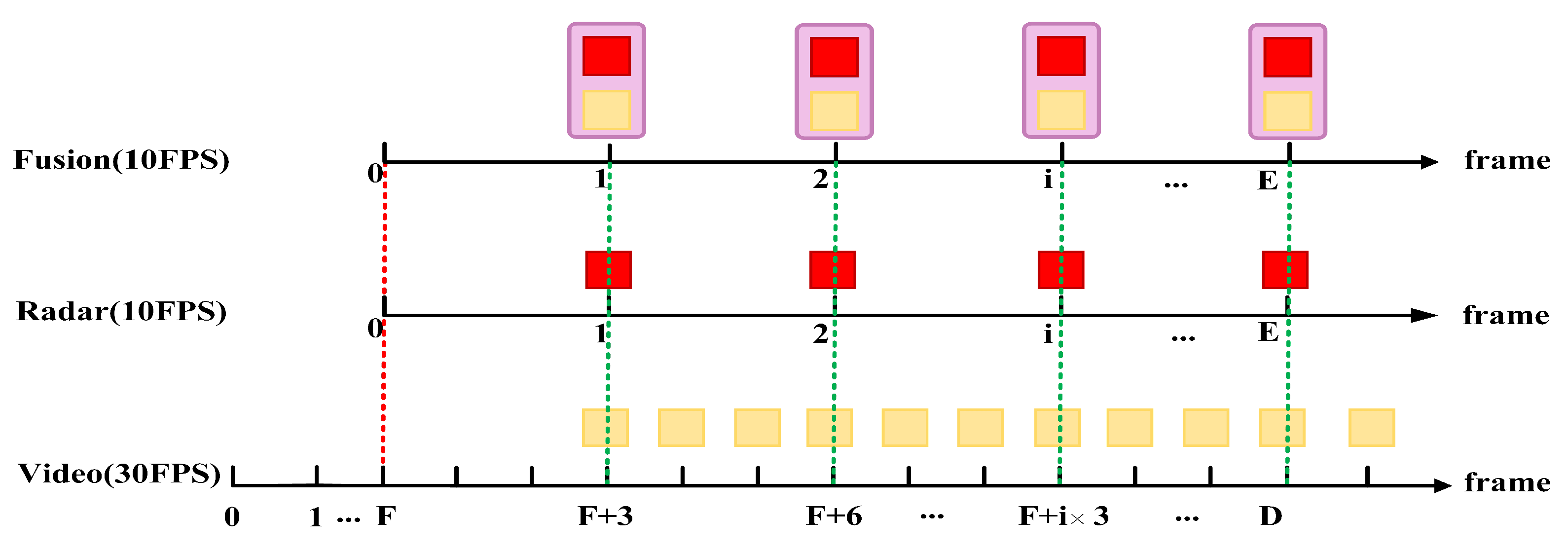
A popular method for aligning the sampling times of multi-sensors is based on timestamps [39]. Because the sampling periods for radar and video are 10 and 30 FPS, we chose that of radar as the baseline. Assume that the starting alignment time of radar and camera is α seconds, the corresponding frame is as follows:
F = α × 30
where the value of α is recorded by the software. Because video has three times the FPS of radar, the frame i of radar data is aligned with the frame F + i × 3 of the image. Figure 5 illustrates the principle of temporal alignment.
The horizontal axis indicates time, which is measured in FPS. The red boxes represent the radar data, the yellow boxes represent the video data, and the purple boxes represent the data after time synchronization.

3.3.2. Spatial Calibration

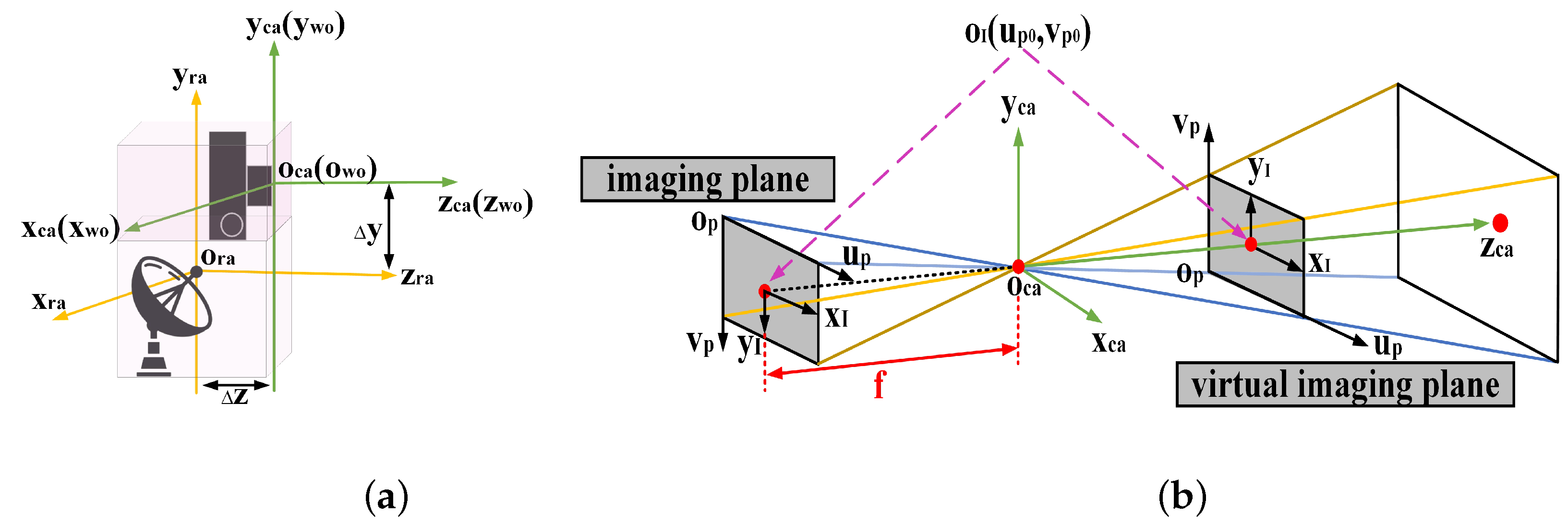
Spatial synchronization involves projecting radar-identified objects onto the image and quantifying their positions in pixels [40]. Figure 6 depicts the basic principle of coordinate transformation.
In this study, we take the world coordinate system as a reference, which is aligned with the camera. Then, the radar coordinate system can be obtained by rotating and translating that of camera. The transformation formula can be expressed as follows:
x ca y ca z ca 1 = R rc T rc 0 T 1 x ra y ra z ra 1
where ( x ca , y ca , z ca ) denotes the coordinates with an origin at the optical center of camera, and ( x ra , y ra , z ra ) denotes the coordinates with origin at the center of radar. R rc denotes a rotational relationship between the camera and radar, and T rc denotes a translational relationship. As shown in Figure 6a, the camera is fitted in the rectangular box to ensure no angular deflection between the two sensors. Thus, R rc is a unit matrix of dimension 3 × 3 . Then, by measuring, we can obtain the elements of the matrix T rc are as follows:
T rc = Δ x Δ y Δ z = 0 180 17
where Δ x , Δ y and Δ z denote the offset of the corresponding coordinate axes between the centers of the radar and the camera, respectively, which are measured in millimeters.
As shown in Figure 6b, a two-dimensional imaging plane is usually used to represent the position of a target in an image. Then, the transformation relationship between the camera coordinate and that of image can be expressed as follows:
z ca x I y I 1 = f 0 0 0 0 f 0 0 0 0 1 0 x ca y ca z ca 1
where f represents the camera’s focal length. However, the above coordinate systems are all in units of length, which are not conducive to subsequent operations. Therefore, it is necessary to convert the image coordinate system o I - x I y I into that of pixel o p - u p v p . These two coordinate systems are in the same plane, and their differences are that they have different origins and units of measurement. Here, the origin o p of the pixel coordinate system is located at the top left corner of the imaging plane, as shown in the shaded portion of Figure 6b. Assuming that the corresponding physical lengths of each pixel on the x I and y I axes are dx and dy , respectively, the coordinate transformation relationship between the image and pixel is as follows:
u p = x I dx + u p 0 v p = y I dy + v p 0
u p v p 1 = 1 dx 0 u p 0 0 1 dy v p 0 0 0 1 x I y I 1
where ( u p 0 , v p 0 ) denotes the position of point o I under the pixel coordinate system. To summarize, the transformation formula from the radar coordinate system to that of the pixel is as follows:
z ca u p v p 1 = f dx 0 u p 0 0 0 f dy v p 0 0 0 0 1 0 R rc T rc 0 T 1 x ra y ra z ra 1
It can be further simplified as:
u p v p 1 = 1 z ca K int K ext x ra y ra z ra 1
K int = f dx 0 u p 0 0 0 f dy v p 0 0 0 0 1 0 = α x 0 u p 0 0 0 α y v p 0 0 0 0 1 0
K ext = R rc T rc 0 T 1 = 1 0 0 0 0 1 0 180 0 0 1 17 0 0 0 1
where K int is the internal parameters matrix of the camera. K ext is the external parameters matrix, which can be measured using the Zhengyou Zhang calibration method [41]. The specific calibration process is as follows:
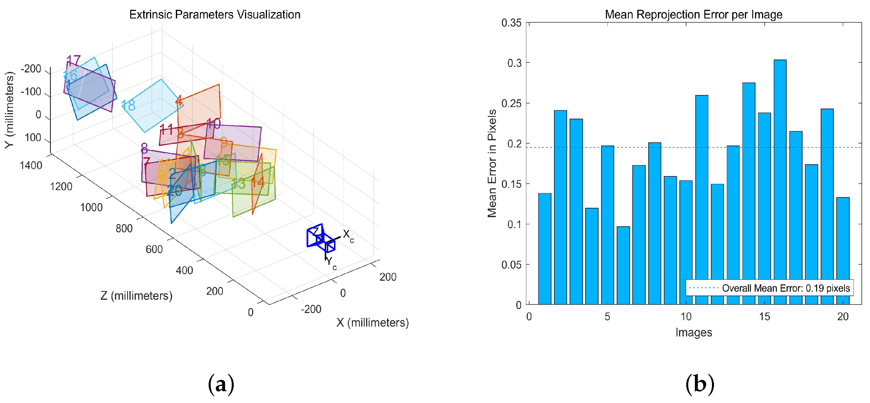
Firstly, a checkerboard with 10 × 8 squares is selected as the calibration board, and the side length of each square is 0.02 m . To obtain calibration results with a high accuracy, we need to take at least 20 images. The calibration images with different angles and attitudes are shown in Figure 7a.
Next, the internal corner points of the checkerboard grid in each image are extracted using the calibration toolbox. Finally, the internal parameters of the camera are derived, as shown in Table 1.
The error of the internal parameters calibration is shown in Figure 7b. Because the average error is within 0.19 pixels, it meets the requirements for practical applications.

3.4. Information Fusion Strategy

At the beginning, we plot the region of interest (ROI) of the radar-detected object on the image. According to the dimensional limits of the outer contour of the vehicle [42], we set the vehicle height to 2.4 m and width to 2.0 m . Thus, the width ( W ra ) and height ( H ra ) of the ROI occupied by the radar point in the imaging plane are as follows:
W ra = 2.4 × α x y ra H ra = 2.0 × α y y ra
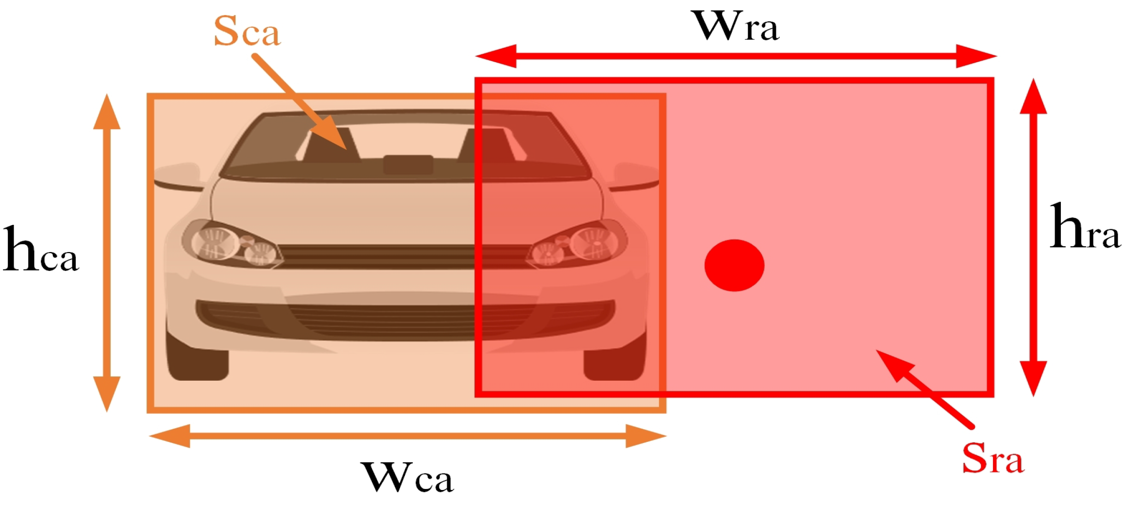
where both ( W ra ) and ( H ra ) are measured in pixels. Assume that the area of the radar ROI is S ra as well as S ca for the camera, as shown in Figure 8. Therefore, the equation for IOU is given below:
IOU = S ra S ca S ra S ca
Then, IOU is used to determine the degree of correlation between objects from the two sensors. The fusion strategy is established as illustrated in Table 2. Where, radar mainly provides the target’s distance, speed, and angle, while the camera mainly provides the category. In addition, if radar misses while the camera detects the target, the distance is provided by the camera.

3.5. Evaluation Indicators

In this study, we choose Precision, Recall, and Balanced-score as performance evaluation indicators [43]. The formulas are as follows:
Precision = TP TP + FP
Recall = TP TP + FN
Balance - score = ( Precision × Recall ) Precision + Recall × 2
where Precision is the correct detection probability. Recall denotes the detection probability. Balance - score is the reconciled average of Precision and Recall . TP indicates the quantity of valid objects that are accurately identified. FP indicates the quantity of invalid objects that are alarmed. FN indicates the quantity of valid objects that have been missed.

4. Results and Discussion

In this section, we analyze the algorithms’ performance in detail, using roads on campus as experimental scenarios. The camera and radar are mounted on the same tripod, and the height of the camera’s optical center from the ground is 1.28 m . The positional relationship between the camera and radar are aligned with those outlined in Section 3.3.2. And, the details of tools and environments are provided in Table 3.

4.1. Validation of YOLOv5s Algorithm

To verify that it is reasonable to adopt YOLOv5s as a visual target detection algorithm, we compared it with several mainstream algorithms, as shown in Figure 9. Where all of the models use pre-trained weights, which are provided by the official [44] and trained on the COCO dataset. Compared with YOLOv8s and YOLOv9s, YOLOv5s performs better in parameters (Params), floating-point operations per second (FLOPs), and FPS. Furthermore, while YOLOv5s has slightly fewer Params and FLOPs than YOLOv7-tiny, its AP value improves by 5.5% relative to YOLOv7-tiny. Therefore, we can conclude that YOLOv5s strikes a balance between spatio-temporal complexity and detection accuracy. The experimental outcomes justify the choice of YOLOv5s to recognize objects captured by the camera.
To validate the performance of YOLOv5s model in practical applications, we use it to process images we have captured ourselves. As illustrated in Figure 10, YOLOv5s performs well despite the targets being in harsh environments, such as exposure, low light, long distance, and partial occlusion.

4.2. Validation of SAO-DBSCAN Algorithm

4.2.1. Comparison with Kmeans Algorithm

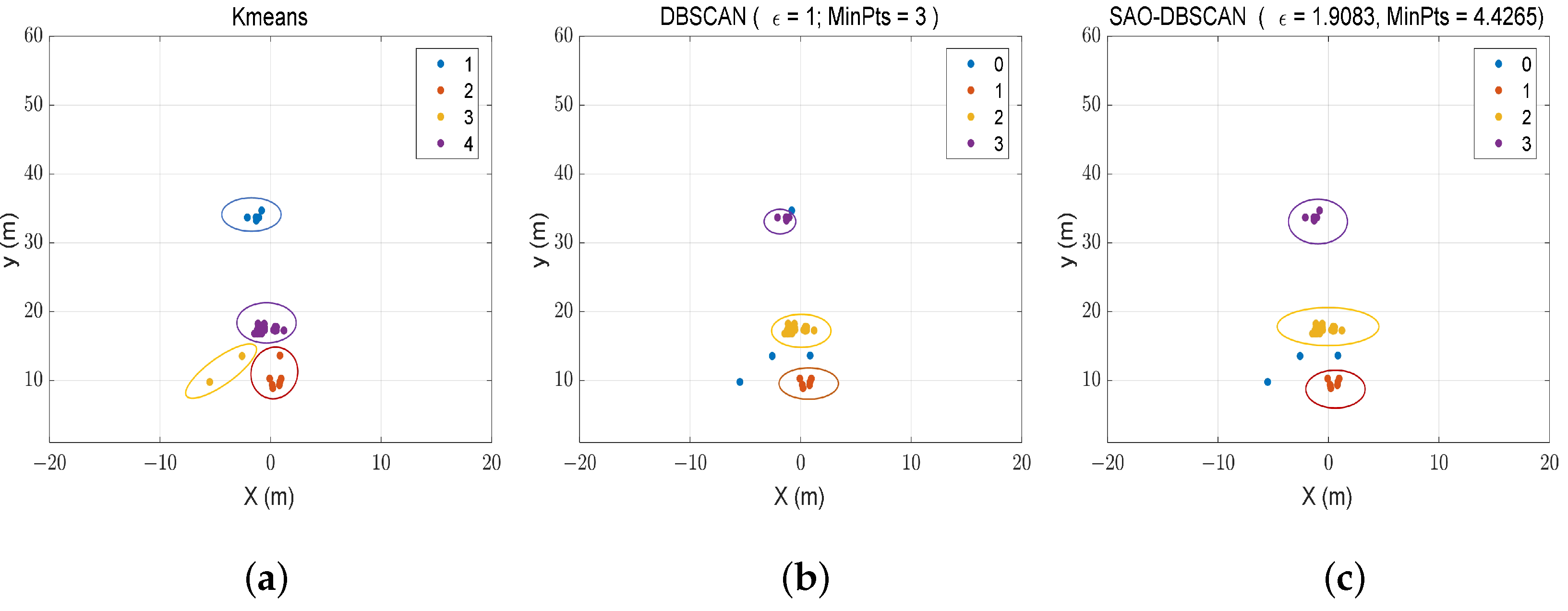
A tripod mounted with a radar and camera was fixed on the road during experiments. And, three stationary targets to be detected were placed at ( 1.10 m , 17.40 m ) , ( 1.18 m , 34.40 m ) , and ( 0.50 m , 9.40 m ) . Then, the information of the objects is pre-processed after collecting them using the radar. Subsequently, different clustering algorithms are used to cluster the radar point clouds, and the results are displayed in Figure 11.
Experiments show that the Kmeans, DBSCAN, and SAO-DBSCAN provide different clustering effects. In Figure 11a, the Kmeans demands the actual quantity of objects to be determined before clustering, but it is impossible for a vehicle-mounted radar. In contrast, the density-based clustering algorithms in Figure 11b,c do not need this information. In the density-based clustering algorithms, clusters are considered to be regions in space that are densely populated with points. On the contrary, low-density points among the clusters are considered as noise. Furthermore, the clusters can take any shape, and the points in the clusters can be distributed arbitrarily. As the density-based clustering algorithms have these features, which are remarkably close to those of targets detected by vehicle-mounted radar, they are preferable for processing data from the vehicle-mounted radar.

4.2.2. Comparison with DBSCAN Algorithm

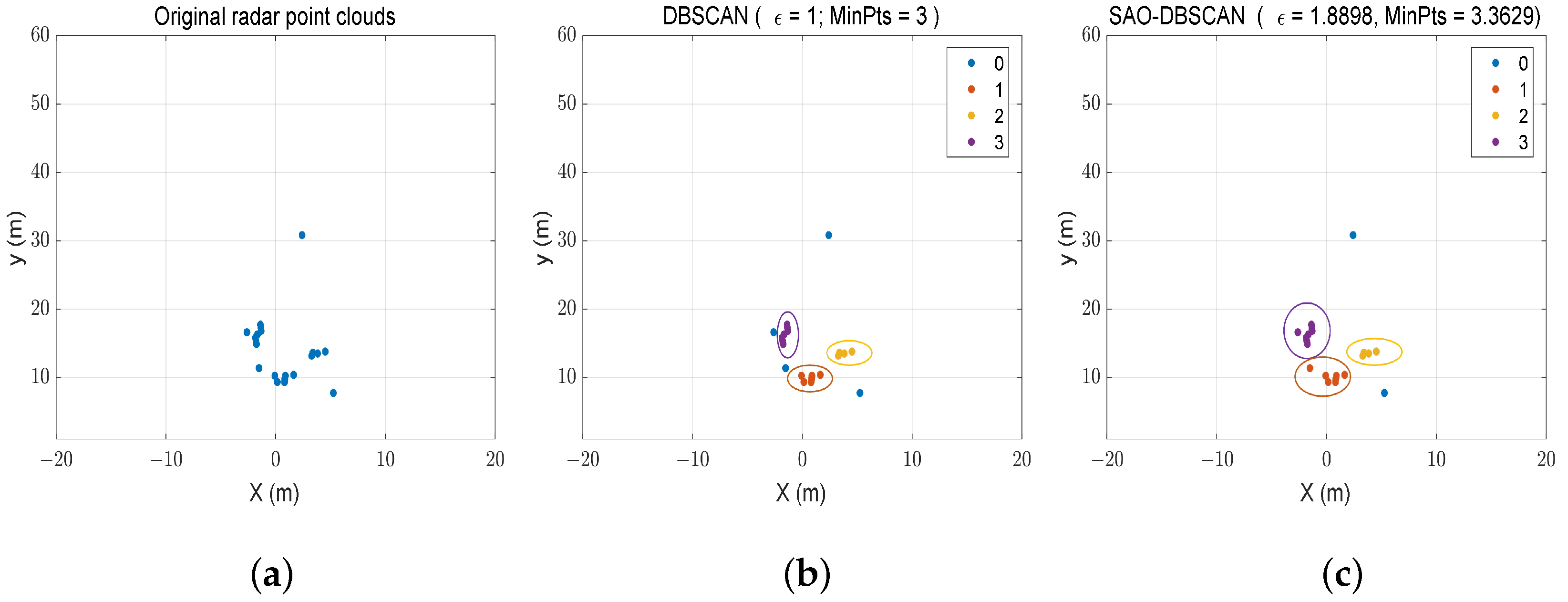
To demonstrate the robustness of SAO-DBSCAN, we use it to process point clouds with fluctuating density. During the experiments, the targets to be detected are constantly kept stationary, and three frames of data are repeatedly captured by radar. The actual positions of the targets are shown in Figure 12.
Figure 13a, Figure 14a and Figure 15a display the original radar point clouds after pre-processing. Experiments show that the density of the point clouds will change in different frames, even if they come from a same target. Subsequently, we obtain different clusters using the traditional DBSCAN and the proposed SAO-DBSCAN. Where the parameters of DBSCAN are ε = 1 and MinPts = 3 , and that of SAO-DBSCAN are L = [ 1 , 3 ] and U = [ 2 , 5 ] . In Figure 13b, DBSCAN can accurately distinguish the boundaries among different targets with the pre-setting parameters. However, in Figure 14b and Figure 15b, the clustering effects of DBSCAN show apparent defects. On the contrary, in Figure 13c, Figure 14c and Figure 15c, the proposed SAO-DBSCAN can automatically solve the optimal values of ε and MinPts so as to correctly distinguish each class of targets.
In the following, we place targets with different reflective properties on the road, aiming to verify the ability of SAO-DBSCAN to distinguish among them. The actual locations of targets are shown in Figure 16.
Figure 17a shows the point clouds after pre-processing and filtering. The cars have multiple reflective surfaces, which will cause the point clouds obtained from the same reflective surface to be dense while those among different reflective surfaces will be discrete. Therefore, the same large target is misreported as multiple targets by DBSCAN, as shown by the arrows in Figure 17b. On the contrary, the proposed SAO-DBSCAN can solve this problem perfectly. It can calculate the optimal values of ε and MinPts according to the reflective properties of the objects so as to classify them correctly. The results can be found in Figure 17c.
In summary, DBSCAN requires pre-setting the specific values of ε and MinPts . When the density of the point clouds fluctuates heavily, its performance will decrease drastically. In contrast, the proposed SAO-DBSCAN only requires a reasonable range of values for the parameters, which are related to the signal reflection performance of the radar. Consequently, it can work in changing scenarios and it exhibits an excellent clustering performance.

4.3. Validation of Information Fusion

4.3.1. Visualization of Information Fusion

Keep the positions of the targets consistent with those depicted in Figure 16 in Section 4.2.2, and collect their information by radar and camera. Then, the targets in the image are extracted using the YOLOv5s model, and the interferences located beyond the lanes are removed. The effective clusters detected by radar are extracted using DBSCAN and SAO-DBSCAN, respectively. Where the clustering results are consistent with those depicted in Figure 17b,c in Section 4.2.2. Subsequently, we calculate the average of the clusters’ coordinates to obtain their exact locations. Finally, the effective targets detected by radar and camera are fused, as illustrated in Figure 18.
Here, the purple bounding boxes indicate that both the two sensors recognize the same objects, and the red boxes indicate that only the radar detects targets. In Figure 18a, there are false severe positives when using DBSCAN to cluster radar point clouds, which will degrade the performance of the decision-level fusion method. On the contrary, the proposed SAO-DBSCAN in Figure 18b can effectively reduce the false alarms from the radar, thus enhancing the accuracy of fusion.

4.3.2. Performance Analysis of Algorithms

For proving the superiority of the fusion model that we suggest, we compare it with other related methods in comparison experiments. Where 199 frames of radar and video data were collected simultaneously for each scenario. Figure 19 demonstrates the details of target movement in various scenarios. Table 4 displays the performance of various algorithms. Where the parameters of DBSCAN are set to ε = 1 and MinPts = 3 , and that of SAO-DBSCAN are set to L = [ 1 , 3 ] and U = [ 2 , 5 ] .
In Table 4, both of these two fusion methods adopt the decision-level strategy. Additionally, ref. [29] uses DBSCAN to cluster the radar point clouds, whereas the proposed fusion model uses SAO-DBSCAN. In Scene 1, the experimental results indicate that the Balance-score for the suggested SAO-DBSCAN shows a 0.02 improvement over DBSCAN. Simultaneously, the fusion method that we suggest demonstrates a 0.01 enhancement compared to [29]. In Scene 2, the Balance-score of SAO-DBSCAN is improved by 0.16 over DBSCAN, and the fusion method is improved by 0.18 over [29]. Therefore, the proposed fusion method is more accurate than other methods in different scenarios.
In addition, comparing the results of Scene 2 with Scene 1, we notice that the generalizability of DBSCAN is poor. With the same parameters, the Balance-score of DBSCAN changes from 0.93 to 0.78, which has a decrease of 0.15. This is due to the fact that the parameters in DBSCAN have to be pre-set, making it difficult to apply in changing situations. Furthermore, because the accuracy of radar decreases dramatically, the Balance-score of the fusion algorithm [29] changes from 0.98 to 0.81, decreasing by 0.16. Conversely, the fluctuation of the Balance-score for the suggested SAO-DBSCAN is only 0.01, as well as that of the proposed fusion algorithm is only 0.02. Consequently, the experiments demonstrate that the fusion algorithm suggested here is robust.
Finally, we provide a detailed analysis of the time and space complexity for the fusion algorithm, illustrated in Table 5. Where 199 frame samples from Scene 1 shown in Figure 19a are used for the evaluation. The experiments indicate that, in comparison with [29], the inferring time for the suggested fusion method rises by just 0.04 s, while the space increases by 10 MB. Therefore, we can conclude that the fusion method suggested here could attain a greater detection accuracy while incurring a slightly larger time and space cost compared to [29].

5. Conclusions

Radar point clouds will experience variations in density, which may cause incorrect alerts during clustering. In turn, it will diminish the precision of the decision-level information fusion method. To address this problem, we suggest a target detection algorithm based on a fusing radar with a camera in the presence of a fluctuating signal intensity. Firstly, we introduce SAO to solve the optimal parameters of DBSCAN, and use the proposed SAO-DBSCAN to cluster the radar point clouds. Then, the YOLOv5s model is employed to identify the objects on the image. Finally, the information of objects detected by radar and vision is fused. The experimental results indicate that the suggested fusion method can attain a Balance-score ranging from 0.97 to 0.99, performing outstandingly in preventing missed detections and false alarms. Additionally, the Balance-score fluctuates within 0.02, indicating that the fusion method is robust. However, it still suffers from the disadvantages of a high spatio-temporal complexity. Therefore, in subsequent endeavors, we will try our best to reduce the time and space overhead while achieving a higher detection accuracy.

Author Contributions

Research design, Y.Y. and X.W. (Xianpeng Wang); data acquisition, X.W. (Xiaoqin Wu), X.L. and Y.G.; writing—original draft preparation, Y.Y.; writing—review and editing, X.W. (Xianpeng Wang), X.L. and T.S.; supervision, X.W. (Xianpeng Wang) and X.W. (Xiaoqin Wu); funding acquisition, X.W. (Xianpeng Wang) and X.L. All authors have read and agreed to the published version of the manuscript.

Funding

This work was supported by the Key Research and Development Project of Hainan Province (ZDYF2023GXJS159), the Natural Science Foundation of Hainan Province (620RC555), and the National Natural Science Foundation of China (No. 61961013, 62101088).

Data Availability Statement

The original contributions presented in the study are included in the article, further inquiries can be directed to the corresponding author.

Conflicts of Interest

The authors declare no conflict of interest.

References

  1. Ansariyar, A.; Taherpour, A.; Masoumi, P.; Jeihani, M. Accident Response Analysis of Six Different Types of Distracted Driving. Komunikácie 2023, 25, 78–95. [Google Scholar] [CrossRef]
  2. Bachute, M.R.; Subhedar, J.M. Autonomous driving architectures: Insights of machine learning and deep learning algorithms. Mach. Learn. Appl. 2021, 6, 100164. [Google Scholar] [CrossRef]
  3. Fernandes, D.; Silva, A.; Névoa, R.; Simões, C.; Gonzalez, D.; Guevara, M.; Novais, P.; Monteiro, J.; Melo-Pinto, P. Point-cloud based 3D object detection and classification methods for self-driving applications: A survey and taxonomy. Inf. Fusion 2021, 68, 161–191. [Google Scholar] [CrossRef]
  4. Hafeez, F.; Sheikh, U.U.; Alkhaldi, N.; Al Garni, H.Z.; Arfeen, Z.A.; Khalid, S.A. Insights and strategies for an autonomous vehicle with a sensor fusion innovation: A fictional outlook. IEEE Access 2020, 8, 135162–135175. [Google Scholar] [CrossRef]
  5. Ravindran, R.; Santora, M.J.; Jamali, M.M. Camera, LiDAR, and radar sensor fusion based on Bayesian neural network (CLR-BNN). IEEE Sens. J. 2022, 22, 6964–6974. [Google Scholar] [CrossRef]
  6. Yeong, D.J.; Velasco-Hernandez, G.; Barry, J.; Walsh, J. Sensor and sensor fusion technology in autonomous vehicles: A review. Sensors 2021, 21, 2140. [Google Scholar] [CrossRef] [PubMed]
  7. Li, Y.; Ibanez-Guzman, J. Lidar for autonomous driving: The principles, challenges, and trends for automotive lidar and perception systems. IEEE Signal Process. Mag. 2020, 37, 50–61. [Google Scholar] [CrossRef]
  8. Şentaş, A.; Tashiev, İ.; Küçükayvaz, F.; Kul, S.; Eken, S.; Sayar, A.; Becerikli, Y. Performance evaluation of support vector machine and convolutional neural network algorithms in real-time vehicle type and color classification. Evolut. Intell. 2020, 13, 83–91. [Google Scholar] [CrossRef]
  9. Duan, J.; Ye, H.; Zhao, H.; Li, Z. Deep Cascade AdaBoost with Unsupervised Clustering in Autonomous Vehicles. Electronics 2022, 12, 44. [Google Scholar] [CrossRef]
  10. Chen, L.; Lin, S.; Lu, X.; Cao, D.; Wu, H.; Guo, C.; Liu, C.; Wang, F.Y. Deep neural network based vehicle and pedestrian detection for autonomous driving: A survey. IEEE Trans. Intell. Transp. Syst. 2021, 22, 3234–3246. [Google Scholar] [CrossRef]
  11. Huang, F.; Chen, S.; Wang, Q.; Chen, Y.; Zhang, D. Using deep learning in an embedded system for real-time target detection based on images from an unmanned aerial vehicle: Vehicle detection as a case study. Int. J. Digit. Earth 2023, 16, 910–936. [Google Scholar] [CrossRef]
  12. Michaelis, C.; Mitzkus, B.; Geirhos, R.; Rusak, E.; Bringmann, O.; Ecker, A.S.; Bethge, M.; Brendel, W. Benchmarking robustness in object detection: Autonomous driving when winter is coming. arXiv 2019, arXiv:1907.07484. [Google Scholar]
  13. Yi, C.; Zhang, K.; Peng, N. A multi-sensor fusion and object tracking algorithm for self-driving vehicles. Proc. Inst. Mech. Eng. Part D J. Automob. Eng. 2019, 233, 2293–2300. [Google Scholar] [CrossRef]
  14. Shi, J.; Wen, F.; Liu, T. Nested MIMO radar: Coarrays, tensor modeling, and angle estimation. IEEE Trans. Aerosp. Electron. Syst. 2020, 57, 573–585. [Google Scholar] [CrossRef]
  15. Shi, J.; Yang, Z.; Liu, Y. On parameter identifiability of diversity-smoothing-based MIMO radar. IEEE Trans. Aerosp. Electron. Syst. 2021, 58, 1660–1675. [Google Scholar] [CrossRef]
  16. Shi, J.; Wen, F.; Liu, Y.; Liu, Z.; Hu, P. Enhanced and generalized coprime array for direction of arrival estimation. IEEE Trans. Aerosp. Electron. Syst. 2022, 59, 1327–1339. [Google Scholar] [CrossRef]
  17. Wei, Z.; Zhang, F.; Chang, S.; Liu, Y.; Wu, H.; Feng, Z. Mmwave radar and vision fusion for object detection in autonomous driving: A review. Sensors 2022, 22, 2542. [Google Scholar] [CrossRef]
  18. Hyun, E.; Jin, Y. Doppler-spectrum feature-based human—Vehicle classification scheme using machine learning for an FMCW radar sensor. Sensors 2020, 20, 2001. [Google Scholar] [CrossRef]
  19. Lu, Y.; Zhong, W.; Li, Y. Calibration of multi-sensor fusion for autonomous vehicle system. Int. J. Veh. Des. 2023, 91, 248–262. [Google Scholar] [CrossRef]
  20. Tang, X.; Zhang, Z.; Qin, Y. On-road object detection and tracking based on radar and vision fusion: A review. IEEE Intell. Transp. Syst. Mag. 2021, 14, 103–128. [Google Scholar] [CrossRef]
  21. Chen, B.; Pei, X.; Chen, Z. Research on target detection based on distributed track fusion for intelligent vehicles. Sensors 2019, 20, 56. [Google Scholar] [CrossRef]
  22. Lv, P.; Wang, B.; Cheng, F.; Xue, J. Multi-objective association detection of farmland obstacles based on information fusion of millimeter wave radar and camera. Sensors 2022, 23, 230. [Google Scholar] [CrossRef] [PubMed]
  23. Jha, H.; Lodhi, V.; Chakravarty, D. Object detection and identification using vision and radar data fusion system for ground-based navigation. In Proceedings of the 2019 6th IEEE International Conference on Signal Processing and Integrated Networks (SPIN), Noida, India, 7–8 March 2019; pp. 590–593. [Google Scholar]
  24. Zewge, N.S.; Kim, Y.; Kim, J.; Kim, J.H. Millimeter-wave radar and RGB-D camera sensor fusion for real-time people detection and tracking. In Proceedings of the 2019 7th IEEE International Conference on Robot Intelligence Technology and Applications (RiTA), Daejeon, Republic of Korea, 1–3 November 2019; pp. 93–98. [Google Scholar]
  25. Jibrin, F.A.; Deng, Z.; Zhang, Y. An object detection and classification method using radar and camera data fusion. In Proceedings of the 2019 IEEE International Conference on Signal, Information and Data Processing (ICSIDP), Chongqing, China, 11–13 December 2019; pp. 1–6. [Google Scholar]
  26. Wang, L.; Zhang, Z.; Di, X.; Tian, J. A roadside camera-radar sensing fusion system for intelligent transportation. In Proceedings of the 2020 17th IEEE European Radar Conference (EuRAD), Utrecht, The Netherlands, 13–15 January 2021; pp. 282–285. [Google Scholar]
  27. Wu, Y.; Li, D.; Zhao, Y.; Yu, W.; Li, W. Radar-vision fusion for vehicle detection and tracking. In Proceedings of the 2023 IEEE International Applied Computational Electromagnetics Society Symposium (ACES), Monterey, CA, USA, 26–30 March 2023; pp. 1–2. [Google Scholar]
  28. Cheng, D.; Xu, R.; Zhang, B.; Jin, R. Fast density estimation for density-based clustering methods. Neurocomputing 2023, 532, 170–182. [Google Scholar] [CrossRef]
  29. Deng, L.; Liu, S. Snow ablation optimizer: A novel metaheuristic technique for numerical optimization and engineering design. Expert Syst. Appl. 2023, 225, 120069. [Google Scholar] [CrossRef]
  30. Peng, D.; Ding, W.; Zhen, T. A novel low light object detection method based on the YOLOv5 fusion feature enhancement. Sci. Rep. 2024, 14, 4486. [Google Scholar] [CrossRef]
  31. YenIaydin, Y.; Schmidt, K.W. A lane detection algorithm based on reliable lane markings. In Proceedings of the 2018 26th IEEE Signal Processing and Communications Applications Conference (SIU), Izmir, Turkey, 2–5 May 2018; pp. 1–4. [Google Scholar]
  32. Yang, Y.; Wang, X.; Wu, X.; Lan, X.; Su, T.; Guo, Y. A Robust Target Detection Algorithm Based on the Fusion of Frequency-Modulated Continuous Wave Radar and a Monocular Camera. Remote Sens. 2024, 16, 2225. [Google Scholar] [CrossRef]
  33. Wu, J.X.; Xu, N.; Wang, B.; Ren, J.Y.; Ma, S.L. Research on Target Detection Algorithm for 77 GHz Automotive Radar. In Proceedings of the 2022 IEEE 16th International Conference on Solid-State & Integrated Circuit Technology (ICSICT), Nangjing, China, 25–28 October 2022; pp. 1–3. [Google Scholar]
  34. Zhao, R.; Yuan, X.; Yang, Z.; Zhang, L. Image-based crop row detection utilizing the Hough transform and DBSCAN clustering analysis. IET Image Process. 2024, 18, 1161–1177. [Google Scholar] [CrossRef]
  35. McCrory, M.; Thomas, S.A. Cluster Metric Sensitivity to Irrelevant Features. arXiv 2024, arXiv:2402.12008. [Google Scholar]
  36. Saleem, S.; Animasaun, I.; Yook, S.J.; Al-Mdallal, Q.M.; Shah, N.A.; Faisal, M. Insight into the motion of water conveying three kinds of nanoparticles shapes on a horizontal surface: Significance of thermo-migration and Brownian motion. Surfaces Interfaces 2022, 30, 101854. [Google Scholar] [CrossRef]
  37. Liu, Y.; Jiang, B.; He, H.; Chen, Z.; Xu, Z. Helmet wearing detection algorithm based on improved YOLOv5. Sci. Rep. 2024, 14, 8768. [Google Scholar] [CrossRef]
  38. Yang, J.; Huang, W. Pedestrian and vehicle detection method in infrared scene based on improved YOLOv5s model. Autom. Mach. Learn. 2024, 5, 90–96. [Google Scholar]
  39. Liu, C.; Zhang, G.; Qiu, H. Research on target tracking method based on multi-sensor fusion. J. Chongqing Univ. Technol. 2021, 35, 1–7. [Google Scholar]
  40. Du, Y.; Qin, B.; Zhao, C.; Zhu, Y.; Cao, J.; Ji, Y. A novel spatio-temporal synchronization method of roadside asynchronous MMW radar-camera for sensor fusion. IEEE Trans. Intell. Transp. Syst. 2021, 23, 22278–22289. [Google Scholar] [CrossRef]
  41. Lu, P.; Liu, Q.; Guo, J. Camera calibration implementation based on Zhang Zhengyou plane method. In Proceedings of the 2015 Chinese Intelligent Systems Conference, Yangzhou, China, 17–18 October 2015; Springer: Berlin/Heidelberg, Germany, 2016; Volume 1, pp. 29–40. [Google Scholar]
  42. Qin, P.; Hou, X.; Zhang, S.; Zhang, S.; Huang, J. Simulation research on the protection performance of fall protection net at the end of truck escape ramp. Sci. Prog. 2021, 104, 00368504211039615. [Google Scholar] [CrossRef] [PubMed]
  43. Zhao, X.; Liu, K.; Gao, K.; Li, W. Hyperspectral time-series target detection based on spectral perception and spatial-temporal tensor decomposition. IEEE Trans. Geosci. Remote Sens. 2023, 61, 5520812. [Google Scholar] [CrossRef]
  44. Wang, C.Y.; Yeh, I.H.; Liao, H.Y.M. Yolov9: Learning what you want to learn using programmable gradient information. arXiv 2024, arXiv:2402.13616. [Google Scholar]
Figure 1. Schematic diagram of multi-sensor fusion.
Remotesensing 16 03356 g001
Figure 2. Three types of points in DBSCAN.
Remotesensing 16 03356 g002
Figure 3. Block diagram of SAO-DBSCAN.
Remotesensing 16 03356 g003
Figure 4. The structure of YOLOv5s.
Remotesensing 16 03356 g004
Figure 5. The principle of temporal alignment.
Remotesensing 16 03356 g005
Figure 6. Schematic diagram of the coordinate transformation. (a) Positional relationship between the radar and camera. (b) Camera imaging model.
Remotesensing 16 03356 g006
Figure 7. The principle of internal parameter calibration. (a) Calibration images for different positions, angles, and attitudes. (b) Error analysis.
Remotesensing 16 03356 g007
Figure 8. ROIs of objects from different sensors.
Remotesensing 16 03356 g008
Figure 9. Performances of different YOLOs.
Remotesensing 16 03356 g009
Figure 10. Performance of YOLOv5s in practical applications. (a) Exposure. (b) Low light. (c) Small target from a distance. (d) Target is partially obscured.
Remotesensing 16 03356 g010
Figure 11. Processing results of different clustering algorithms. (a) Kmeans. (b) DBSCAN. (c) SAO-DBSCAN.
Remotesensing 16 03356 g011
Figure 12. Density of the same target fluctuates.
Remotesensing 16 03356 g012
Figure 13. Clustering results for the first frame. (a) Original radar point clouds. (b) DBSCAN. (c) SAO-DBSCAN.
Remotesensing 16 03356 g013
Figure 14. Clustering results for the second frame. (a) Original radar point clouds. (b) DBSCAN. (c) SAO-DBSCAN.
Remotesensing 16 03356 g014
Figure 15. Clustering results for the third frame. (a) Original radar point clouds. (b) DBSCAN. (c) SAO-DBSCAN.
Remotesensing 16 03356 g015
Figure 16. Reflectivity of different targets varies.
Remotesensing 16 03356 g016
Figure 17. Clustering results for targets with different reflectivity. (a) Original radar point clouds. (b) DBSCAN. (c) SAO-DBSCAN.
Remotesensing 16 03356 g017
Figure 18. Visualization of multi-sensor fusion. (a) Fusion results after clustering radar point clouds with DBSCAN. (b) Fusion results after clustering radar point clouds with SAO-DBSCAN.
Remotesensing 16 03356 g018
Figure 19. Details of target movement. (a) Scene 1. (b) Scene 2.
Remotesensing 16 03356 g019
Table 1. Calibration results of the internal camera parameters.
Internal ParametersHorizontal Axis/PixelVertical Axis/Pixel
Equivalent focal length α x = 1545.9 α y = 1550.4
Principal point u p 0 = 1001.1 v p 0 = 529.5
Table 2. Targets detection accuracy in different environments.
Value of IOUInformation on the Bounding BoxSensor Detection ResultsOutput
IOU 0 S ra 0 , S ca 0 Both radar and camera recognize the same object.Output the valid information recognized by radar and camera.
IOU = 0 S ra = 0 , S ca 0 Radar misses the target.Output the valid information detected by camera.
S ra 0 , S ca = 0 camera misses the target.Output the valid information detected by radar.
S ra = 0 , S ca = 0 There is no target.There is no information to output.
Table 3. Details of tools and environments.
NameVersionFunction
RadarTexas Instruments (TI) AWR2243- -
CameraHewlett-Packard (HP) 1080p- -
GPUNVIDIA GeForce RTX 3060- -
CPUi5-11400- -
Operating systemWindows11- -
Python3.8- -
Pytorch11.3- -
CUDA12.3- -
Pycharm2023Running YOLOs for detecting targets in images
MATLABR2022bRunning radar and fusion algorithms
Table 4. Performance of various algorithms.
Detection SceneAlgorithmSensors Combination SolutionsRecallPrecisionBalance-Score
Scene 1DBSCANradar95.24%90.70%0.93
SAO-DBSCANradar99.26%90.93%0.95
Fusion [29]Camera-radar99.31%97.96%0.98
Fusion (ours)Camera-radar99.08%97.96%0.99
Scene 2DBSCANradar94.87%66.82%0.78
SAO-DBSCANradar93.53%95.44%0.94
Fusion [29]Camera-radar99.11%68.10%0.81
Fusion (ours)Camera-radar99.11%95.59%0.97
Table 5. Spatio-temporal complexity analysis.
AlgorithmTime Overhead/sSpace Overhead/MB
Fusion [29]0.941291
Fusion (ours)0.901301
Disclaimer/Publisher’s Note: The statements, opinions and data contained in all publications are solely those of the individual author(s) and contributor(s) and not of MDPI and/or the editor(s). MDPI and/or the editor(s) disclaim responsibility for any injury to people or property resulting from any ideas, methods, instructions or products referred to in the content.