Cluster-Based Wood–Leaf Separation Method for Forest Plots Using Terrestrial Laser Scanning Data

Abstract

Successfully separating wood and leaves in forest plots is a prerequisite for measuring structural parameters and reconstructing 3D forest models. Terrestrial laser scanning (TLS) can distinguish between the leaves and wood of trees through precise and dense point clouds. However, most existing wood–leaf separation methods face significant accuracy issues, especially in dense forests, due to the complications introduced by canopy shading. In this study, we propose a method to separate the wood and leaves in forest plots using the clustering features of TLS data. The method first filters a point cloud to remove the ground points, and then clusters the point cloud using a region-growing algorithm. Next, the clusters are processed based on their sizes and numbers of points for preliminary separation. Chaos Distance is introduced to characterize the observation that wood points are more orderly while leaf points are more chaotic and disorganized. Lastly, the clusters’ Chaos Distance is used for the final separation. Three representative plots were used to validate this method, achieving an average accuracy of 0.938, a precision of 0.927, a recall of 0.892, and an F1 score of 0.907. The three sample plots were processed in 5.18, 3.75, and 14.52 min, demonstrating high efficiency. Comparing the results with the LeWoS and RF models showed that our method better addresses the accuracy issues of complex canopy structures.

1. Introduction

Effective management and conservation of forests, which are crucial for climate regulation, carbon cycling, and biodiversity preservation, require a precise understanding of their structural dynamics and compositions [1,2]. Accurate separation of wood and leaves is a critical step in forest ecology studies, particularly for calculating important parameters like the Leaf Area Index (LAI), Leaf Area Density (LAD), Aboveground Biomass (AGB), and so on. These parameters are foundational for understanding forest structure and health. Additionally, accurate separation is necessary for advanced tasks such as tree skeleton extraction and 3D reconstruction, which require high-quality input data [3]. Therefore, the precision of these subsequent tasks is closely linked to the accuracy of wood–leaf separation. Traditional methods primarily rely on manual leaf extraction, which is both costly and time-consuming. With the development of passive remote sensing technology (e.g., photogrammetric techniques), the efficiency of wood–leaf separation can be improved by applying Computer Vision (CV) theory combined with digital image processing [4,5,6]. However, these techniques have poor penetration abilities and cannot detect the interior of the canopy [7,8].

Light Detection and Ranging (LiDAR) is an emerging technology that offers high-precision active remote sensing detection. It is a powerful optical sensing technology that uses a laser as an emitting light source to measure the distance and other characteristics of a target object [9,10]. It works by emitting a laser signal in the green or near-infrared band towards a target. Then, it compares the received signal reflected from the target (target echo) with the transmitted signal. Relevant information about the target can be obtained after appropriate processing [11,12]. Compared to data collected using other remote sensing methods, LiDAR data provide more realistic depictions of object surfaces, morphologies, and other relevant details [9,13]. Terrestrial Laser Scanning (TLS) is a type of LiDAR that generates denser and more detailed point clouds compared to Backpack Laser Scanning (BLS), Uncrewed Aerial Vehicle Laser Scanning (ULS), and Airborne Laser Scanning (ALS). This high level of detail makes TLS data suitable for achieving wood–leaf separation [14].

TLS point cloud data contain 3D coordinates and intensity information for each point. At present, wood–leaf separation technology is mature for individual trees. However, the separation of the wood and leaves of individual trees cannot meet the needs of practical applications most of the time. In addition, when it comes to forest plots, the processing speed is slow due to the large amounts of data. Therefore, it is important to achieve efficient wood–leaf separation in forest plots. Methods for wood–leaf separation can be categorized into two types: those using a combination of radiation and geometric features and those using only geometric features [15]. Effective wood–leaf separation can be achieved by simultaneously analyzing the intensity and 3D coordinate differences between wood and leaves [16,17,18]. Despite its theoretical accuracy, applying this method to actual forest plots faces challenges, primarily due to the sensitivity of the intensity differences to various conditions [19]. To generalize these kinds of methods to actual forest plots, they still need to address the issue of intensity variability.

Geometric features are commonly used for wood–leaf separation and can be categorized based on their foci as graph-based features, local neighborhood features, and cluster-based features [15,20]. Graph-based features include the shortest paths and the mode point of the data. Multiple studies have shown that these parameters can be used to achieve high accuracy in wood–leaf separation [20,21,22]. Hui et al. [20] proposed a separation method based on the evolution of mode points with an average Kappa of 0.771. Tian et al. [21] proposed a graph-based wood–leaf separation (GBS) method that synthesizes the advantages of several existing wood–leaf separation methods by making full use of shortest path information. The average accuracy of GBS has reached 0.94, which is significantly better than those of other mainstream methods. However, existing graph-based methods have primarily been applied to single trees, and their application to forest plots has not yet been validated. Additionally, these methods often require empirical thresholds and are complex in principle [20,21].

The method based on local neighborhood features evaluates the geometric features of each point’s neighbors to achieve wood–leaf separation. The main parameters are the normal vector difference and the local density [23,24,25]. Separation using these features combined with machine learning has also been performed [24,25,26]. However, machine learning requires a large amount of data for manual training and a significant initial investment in terms of effort and time for program design [27,28]. The method based on local neighborhood features focuses on and fully utilizes the differences in the morphological characteristics of wood and leaves. Zhu et al. [24] proposed an adaptive radius-based local neighborhood search approach for forest location clouds combined with a Random Forest (RF) model. Moorthy et al. [26] proposed a method for wood–leaf separation that combines the geometric features defined by the radial boundary of the nearest neighbors in a machine learning model. The above studies have indicated that machine learning techniques based on local neighborhood features are feasible for wood–leaf separation and achieve high accuracy. However, these methods usually lack good transferability between different tree species and are significantly inefficient. While local neighborhood-based methods are generally easier to understand than graph-based methods, they require features to be extracted for many points, making them less efficient overall [24,26].

Cluster-based feature methods categorize a point cloud into clusters with similar attributes, then designate these clusters as either wood or leaves [29]. The main clustering methods for point clouds are Euclidean Clustering (EC), density clustering (e.g., Density-Based Spatial Clustering of Applications with Noise (DBSCAN)), hypervoxel clustering, K-Means, etc. [30,31]. Tan et al. [32] used geometric quantities that were derived by setting a threshold to separate leaves from wood. Wan et al. [33] proposed a segment-wise classification method where a point cloud was segmented into multiple small segments, and each segment was classified as wood or leaf based on its geometric features. LeWoS, an open-source method for wood–leaf separation in forest plots, has the advantage that wood–leaf separation can be completed with comparatively high accuracy [3,29]. The rationale for these methods is easier to understand compared to graph-based and local neighborhood feature-based methods. However, these methods have two obvious drawbacks: (1) they ignore differences in leaf and wood morphology, focusing only on geometric features, and (2) they are sensitive to canopy shading when identifying clusters, making separation difficult in dense forests.

To address the issues of inaccuracy in canopy shading situations and inefficiency, this study proposes a new method for separating wood and leaves in forest plots based on cluster features. This method efficiently achieves wood–leaf separation while maintaining high accuracy, particularly in dense forests. This study uses curvature-based regional growth clustering to demonstrate the effectiveness of normal vectors in wood and leaf segmentation. A new cluster parameter called Chaos Distance is proposed. Combined with cluster size and the number of points, Chaos Distance facilitates wood–leaf separation in forest plots. Additionally, we compare the proposed method with the classical LeWoS algorithm and the RF model to highlight its advantages.

2. Selection of Sample Plots

In order to verify the robustness of the proposed method, we selected data from three locations for wood–leaf separation. Overall, the three locations varied significantly, primarily in terms of geographic location, canopy density, tree species, and point cloud density. In this study, a typical plot was selected for accuracy assessment in each of the three locations, representing a broad range of broadleaf forests. The locations and topographies of the three plots are shown in Figure 1. We calculated the LAI and crown cover values in the three plots using the point cloud data processing and analysis software LiDAR360 V7.0 [34]. A summary of the sample plots is shown in

Table 1. Summary of sample plot information.

	Location	Size of Plot (m)	Number of Points	Point Density (Points/m2)	Number of Trees	LAI	Canopy Cover
Plot 1	China	18.71 × 18.43	5,042,403	24,413	44	4.57	0.767
Plot 2	Australia	52.23 × 54.44	6,388,675	4934	42	1.438	0.272
Plot 3	Germany	24.73 × 19.45	8,833,993	18,366	35	9.49	0.964

.

The sample from Plot 1 was collected by the authors at the University of Electronic Science and Technology of China (UESTC) in Chengdu City, Sichuan Province, China (Figure 1a). The plot was scanned multiple times using a Leica ScanStation C10 scanner made in Heerbrugg, Switzerland. It operates with a green laser (532 nm) and a minimum spot spacing of <1 mm. The predominant tree species in this plot was Phoebe Zhennan S. K. Lee. The trees had large numbers of branchlets, which were generally thin. The plot size was 18.71 m × 18.43 m. It comprised 5,042,403 points, with an average point density of approximately 24,413 points/m², and there were 44 clearly identifiable larger trees. This plot had an LAI of approximately 4.57 and a crown cover of approximately 0.767. The average height of the trees in this plot was approximately 8 m. The average DBH of the trees in this plot was approximately 20 cm. Because it was a planted forest, its trees were evenly and uniformly distributed, with moderate spacing between them.

The sample from Plot 2 in Victoria, Australia, corresponded to a publicly available dataset that accurately represented a native eucalypt open forest ecosystem (Figure 1b). The predominant tree species in this plot was Eucalyptus leucoxylon. This species is an evergreen woody tree. A single-station scan of Plot 2 was performed using an RIEGL VZ-400 made in Beijing, China. It works in the near-infrared band at 1550 nm. Specifically, the forest area in this dataset was classified as a dry sclerophyll box–ironbark forest [35]. A portion of the dataset was selected for experimental purposes. In the plot selected for the experiment, the average tree height was approximately 20 m and the average DBH was approximately 25 cm. The size of the plot was 52.23 m × 54.44 m. It comprised 6,388,675 points, with an average point density of approximately 4934 points/m², and there were 42 clearly identifiable larger trees. This plot had an LAI of approximately 1.438 and a crown cover of approximately 0.272. The tree distribution was relatively sparse, with greater space between the trees than in Plot 1. Each tree had fewer leaves, resulting in a lower overall crown cover.

The sample from Plot 3 was from a publicly available dataset from the Bretten municipal forest in the federal state of Baden-Württemberg, Germany (Figure 1c) [36]. The plot was scanned by multiple stations as well as an RIEGL VZ-400. For the experiment, a portion of the dataset from BR03 was selected. In this plot, the average tree height was approximately 24 m. The thickest trees had DBH values of approximately 72 cm, and the thinner ones had values of only 15 cm. The size of the plot was 24.73 m × 19.45 m. It comprised 8,833,993 points, with an average point density of approximately 18,366 points/m², and there were 35 clearly identifiable larger trees. This plot had an LAI of approximately 9.49 and a crown cover of approximately 0.964. Since it was a natural forest, it starkly contrasted with the neat, orderly, and unified forest of Plot 1. In this plot, the tree distribution was relatively dense, with various tree species present, and the overall canopy cover in this region was relatively high.

3. Methods

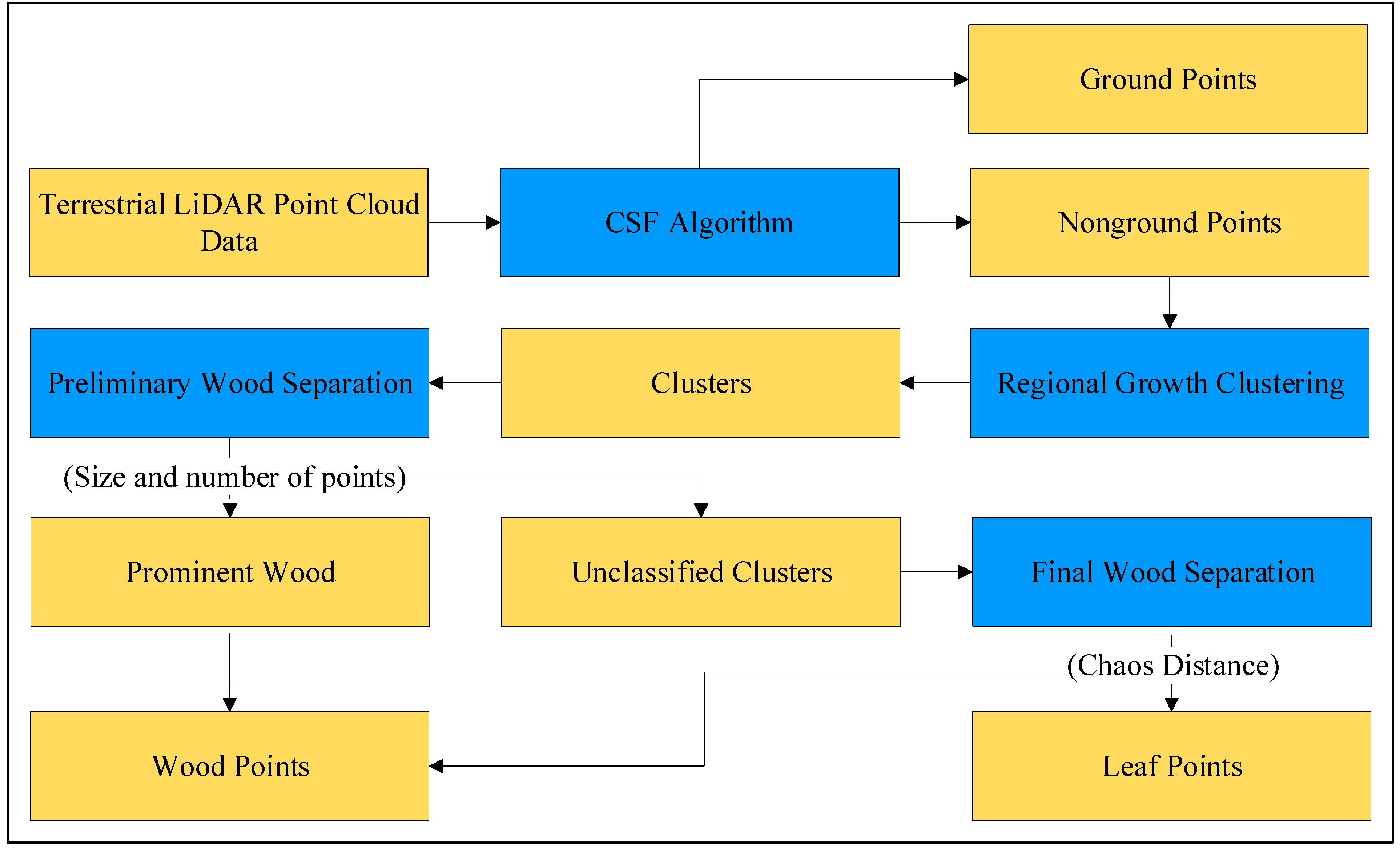
The method proposed in this study uses cluster size, the number of points, and Chaos Distance as key criteria for point cloud classification and separation. This method has four main steps (Figure 2). First, the point cloud is filtered using the Cloth Simulation Filtering (CSF) method, which mainly removes ground points to minimize their interference in the subsequent process [37]. Second, the point cloud is clustered using a region-growing algorithm. It can put wood and leaves in different clusters for better identification. Third, preliminary separation is performed based on size and the number of points, which mainly extracts obvious wood (i.e., the main trunk and the thicker branches of a tree). Finally, the refined final wood separation is accomplished based on the Chaos Distance of the clusters. Chaos Distance is employed to depict the distinct characteristics of wood and leaves in TLS data. In other words, wood tends to exhibit a more uniform morphology, whereas leaves typically display a more erratic distribution. This parameter is used to complete the classification in this step.

3.1. Extraction of Nonground Points

This step involves preprocessing the TLS data, primarily removing the ground points in the plots to reduce their interference in the subsequent process. Most traditional filtering algorithms use differences in slope, elevation, and other parameters to distinguish ground points from nonground points. However, the CSF algorithm proposed by Zhang et al. [37] introduced a new idea for filtering ground points. Currently, the CSF algorithm is widely used to remove ground points from point clouds because it has fewer parameter settings and higher accuracy [37,38].

The algorithm first inverts a point cloud and then assumes that a piece of cloth falls from above due to gravity, so the final position of the cloth represents the current sample terrain. It considers that the fabric particles are affected by both internal and external forces. In this study, the ground points in the three sample plots were effectively removed using this algorithm.

3.2. Point Cloud Clustering

This step involves clustering a preprocessed forest point cloud and grouping morphologically similar points into the same cluster. Due to the significant morphological differences between wood and leaves, clustering can be used to group them into different clusters. This step aims to separate wood and leaf points into different clusters in preparation for the subsequent separation process.

The region-growing clustering algorithm can be used to separate wood and leaves into different clusters. The fundamental principle of regional growth is to aggregate points with similar characteristics to form cohesive regions [30,39]. The resulting clusters are organized into one set or multiple sets through curvature-based region growth clustering, each representing a smooth surface. First, the normal vectors are calculated by selecting neighborhood points, computing the covariance matrix, and performing eigenvalue decomposition to identify the normal vectors based on the local point cloud geometry. The directions of the normal vectors are then determined based on the angles between the lines [30]. A region needs to grow from the point with the smallest curvature value because this point is in a flat region (growing from the flattest area can reduce the total number of line segments). Therefore, a point cloud sorts its points by curvature value [40,41].

Subsequently, for a sorted point cloud (${\mathrm{P}}_{\mathrm{sorted}}$), we select the point with the smallest curvature value (${\mathrm{P}}_{\min }$) as the starting seed point and initialize the current region (${\mathrm{R}}_{\mathrm{c}}$) and current seed list (${\mathrm{S}}_{\mathrm{c}}$). The algorithm starts from the seed point and finds the set of nearest neighbors through a neighborhood lookup. For each nearest neighbor point (${\mathrm{P}}_{\mathrm{j}}$), we check that it satisfies the following two conditions:

• Whether the ${\mathrm{P}}_{\mathrm{j}}$ is still in the untreated ${\mathrm{P}}_{\mathrm{sorted}}$;
• Whether the angle ${\mathsf{\theta }}_{\mathrm{ij}}$ satisfies ${\mathsf{\theta }}_{\mathrm{ij}}<{\mathsf{\theta }}_{\mathrm{th}}$, where ${\mathsf{\theta }}_{\mathrm{ij}}$ is the angle between the ${\mathrm{P}}_{\min }$ and the ${\mathrm{P}}_{\mathrm{j}}$ in the normal vectors’ direction and ${\mathsf{\theta }}_{\mathrm{th}}$ is the preset angle threshold.

If the conditions are met, the ${\mathrm{P}}_{\mathrm{j}}$ is added to the ${\mathrm{R}}_{\mathrm{c}}$ and removed from the ${\mathrm{P}}_{\mathrm{sorted}}$. Otherwise, if the curvature value of the ${\mathrm{P}}_{\mathrm{j}}$ (${\mathrm{cP}}_{\mathrm{j}}$) is less than the curvature threshold (${\mathrm{cP}}_{\mathrm{th}}$), the ${\mathrm{P}}_{\mathrm{j}}$ is added to the ${\mathrm{S}}_{\mathrm{c}}$. The algorithm continuously expands the ${\mathrm{R}}_{\mathrm{c}}$, aggregating points with less curvature and similar normal vector directions into the same region. The iterative process of the algorithm is expressed through the following formulas and conditions:

$${\mathsf{\theta }}_{\mathrm{ij}}={\cos }^{-1}\left(\left|{\overrightarrow{\mathrm{N}}}_{{\mathrm{P}}_{\min }}\cdot {\overrightarrow{\mathrm{N}}}_{{\mathrm{P}}_{\mathrm{j}}}\right|\right)$$

(1)

$${\mathrm{cP}}_{\mathrm{j}}<{\mathrm{cP}}_{\mathrm{th}}$$

(2)

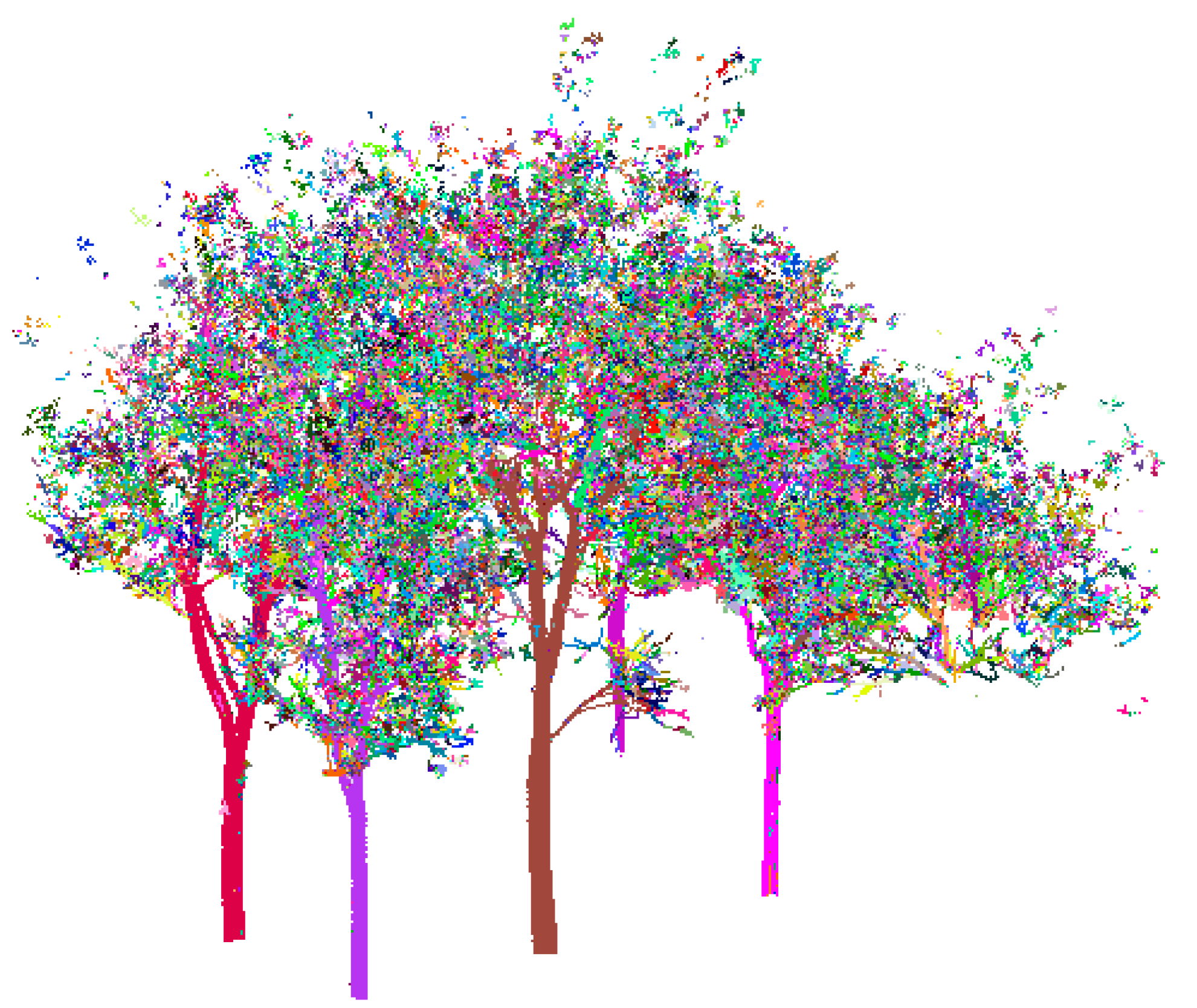
Eventually, the algorithm outputs a global list of segments (R) containing localized regions with similar curvatures and normal vectors [30]. The partial results of this algorithm are visualized in Figure 3, where each color represents a local cluster.

3.3. Preliminary Wood Separation

The purpose of this step is to preliminarily isolate clusters of prominent wood parts, such as the main trunk of a tree, as well as the more obvious thicker branches.

To optimize computational efficiency, preliminary separation prioritizes the identification of distinct wood clusters using relatively simple and computationally fast parameters, such as size and the number of points. During region-growing clustering, it is essentially impossible to cluster a large number of leaf points (i.e., many leaves) into a single cluster due to the utilization of normal vector features.

Therefore, if a cluster contains a large number of points, it is considered a wood cluster. Additionally, leaf clusters are unlikely to have significant height differences along the z-axis, whereas this feature is evident in the trunk. If a cluster has a large height difference, i.e., a large difference in the z-axis direction, it is considered a wood cluster. This can be expressed as follows:

$${\mathrm{W}}_{\mathrm{p}}=\left\{{\mathrm{C}|\mathrm{Z}}_{\mathrm{c}}>{\mathrm{Z}}_{\mathrm{t}},{\mathrm{or}\mathrm{N}}_{\mathrm{c}}>{\mathrm{N}}_{\mathrm{t}}\right\}$$

(3)

where ${\mathrm{W}}_{\mathrm{p}}$ denotes the preliminarily separated wood, $\mathrm{C}$ denotes the clusters, ${\mathrm{Z}}_{\mathrm{t}}$ denotes the difference between the class clusters in the Z-axis direction, ${\mathrm{N}}_{\mathrm{c}}$ denotes the number of points in the clusters, ${\mathrm{Z}}_{\mathrm{t}}$ denotes the threshold value set for the class clusters in the Z-axis direction, and ${\mathrm{N}}_{\mathrm{t}}$ denotes the threshold value set for the number of points. In general, setting ${\mathrm{Z}}_{\mathrm{t}}$ to 2.5 m and ${\mathrm{N}}_{\mathrm{c}}$ to 5000 means that misclassification of leaves can be avoided in this step with better separation of obvious wood.

3.4. Final Wood Separation

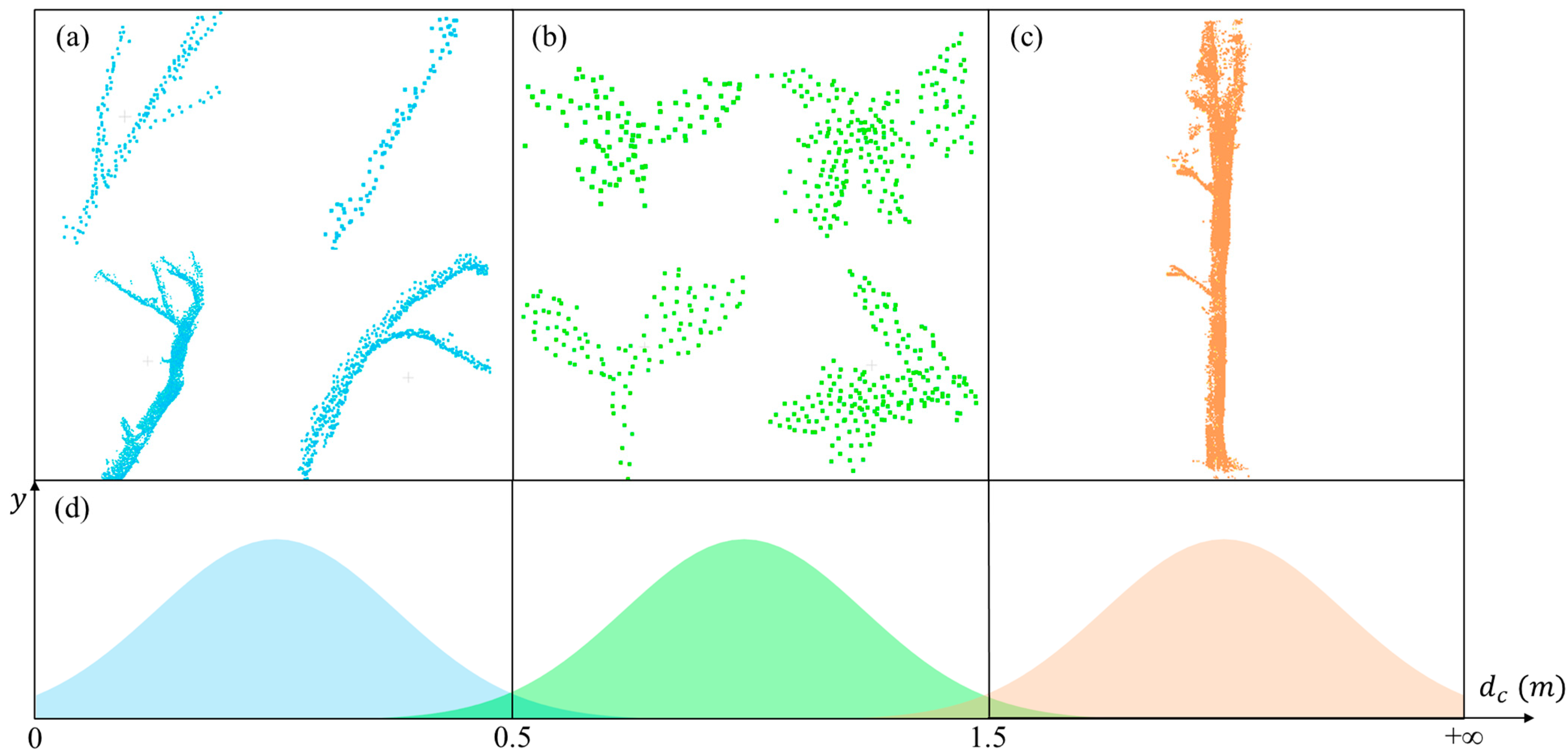
After preliminary wood separation, a more refined extraction and separation process is conducted. The purpose of this step is to classify all clusters that were not classified in the previous step as wood or leaf clusters. After preliminary separation, the remaining cluster types can be grouped into three categories, as shown in Figure 4: clusters containing mainly branches, clusters containing single leaves or a few leaves, and clusters containing mainly trunks. The characteristic that emerges here is a gradual increase in disorganization. We find that we can express this feature with the help of root-mean-square error ($\mathrm{RMSE}$) calculation. In statistics, $\mathrm{RMSE}$ is a good indicator of the precision of a measurement and is calculated as follows:

$$\mathrm{RMSE}=\sqrt{{\displaystyle \frac{{\sum }_{\mathrm{i}=1}^{\mathrm{n}}{\left({\mathrm{X}}_{\mathrm{obs},\mathrm{i}}-{\mathrm{X}}_{\mathrm{model},\mathrm{i}}\right)}^2}{\mathrm{n}}}}$$

(4)

In this equation, ${\mathrm{X}}_{\mathrm{obs},\mathrm{i}}$ and ${\mathrm{X}}_{\mathrm{model},\mathrm{i}}$ refer to the observed and predicted values of the ith data, respectively, and $\mathrm{n}$ is the number of observation points.

This equation cannot be used directly in a point cloud. There are some methods that can fit the model in a point cloud, such as least squares, random sample consensus (RANSAC), etc., but these methods require large computational resources and can directly affect efficiency. Therefore, we chose to process cluster point clouds directly. If a point cloud is considered a “model”, the error between the observed and modeled points can be expressed as follows:

$${\mathrm{E}}_{\mathrm{i},\mathrm{j}}=\sqrt{{\displaystyle \frac{{({\mathrm{X}}_{\mathrm{i}}-{\mathrm{X}}_{\mathrm{j}})}^2+{({\mathrm{Y}}_{\mathrm{i}}-{\mathrm{Y}}_{\mathrm{j}})}^2+{({\mathrm{Z}}_{\mathrm{i}}-{\mathrm{Z}}_{\mathrm{j}})}^2}{3}}}$$

(5)

The above equation represents the error of the ith point with respect to the jth point, where ${\mathrm{X}}_{\mathrm{i}},{\mathrm{Y}}_{\mathrm{i}},{\mathrm{Z}}_{\mathrm{i}},{\mathrm{X}}_{\mathrm{j}},{\mathrm{Y}}_{\mathrm{j}},{\mathrm{and}\mathrm{Z}}_{\mathrm{j}}$ are the $\mathrm{X},\mathrm{Y},\mathrm{and}\mathrm{Z}$ coordinates of the ith and jth points.

Iteration continues through all points in a cluster using the above equation, and results accumulate. Metrics are calculated from these accumulated results to assess the point cloud disorder within a cluster. After bringing the dimensions (units) of all variables into the equation, the final result is expressed in meters (m). Therefore, we named it the Chaos Distance (${\mathrm{d}}_{\mathrm{c}}$). After removing constants that may affect computational efficiency and simplifying the formula, the following equation can be obtained:

$${\mathrm{d}}_{\mathrm{c}}={\displaystyle \frac{2\ast {\sum }_{\mathrm{i}=1}^{\mathrm{n}-1}{\sum }_{\mathrm{j}=\mathrm{i}+1}^{\mathrm{n}}\sqrt{{\left({\mathrm{X}}_{\mathrm{i}}-{\mathrm{X}}_{\mathrm{j}}\right)}^2+{\left({\mathrm{Y}}_{\mathrm{i}}-{\mathrm{Y}}_{\mathrm{j}}\right)}^2+{\left({\mathrm{Z}}_{\mathrm{i}}-{\mathrm{Z}}_{\mathrm{j}}\right)}^2}}{\mathrm{n}\ast \left(\mathrm{n}+1\right)}}$$

(6)

where the unit of ${\mathrm{d}}_{\mathrm{c}}$ is meters ($\mathrm{m}$); $\mathrm{n}$ is the number of points in the class cluster; ${\mathrm{X}}_{\mathrm{i}},{\mathrm{Y}}_{\mathrm{i}},{\mathrm{Z}}_{\mathrm{i}},{\mathrm{X}}_{\mathrm{j}},{\mathrm{Y}}_{\mathrm{j}},{\mathrm{and}\mathrm{Z}}_{\mathrm{j}}$ are the $\mathrm{X},\mathrm{Y},\mathrm{and}\mathrm{Z}$ coordinates of the ith and jth points; and $\mathrm{i}\mathrm{and}\mathrm{j}$ are counted in $\mathrm{n}$. In practice, the calculated ${\mathrm{d}}_{\mathrm{c}}$ is generally multiplied by a scaling factor to amplify the differences between the data, leading to better separation. This scaling factor is generally 10.

It is intuitive to think that the ${\mathrm{d}}_{\mathrm{c}}$ becomes progressively larger from (a) to (c) in the types of clusters represented in Figure 4. Specifically, among similarly sized clusters, wood clusters appear denser and more organized, while leaf clusters are looser and more disorganized. Therefore, for similar-sized clusters, the ${\mathrm{d}}_{\mathrm{c}}$ of wood is smaller than the ${\mathrm{d}}_{\mathrm{c}}$ of leaves. As mentioned in Section 3.2, it is rare for a large number of leaves to be clustered together. At the same time, the class composed of trunks is significantly larger than case (b) in Figure 4 when ${\mathrm{E}}_{\mathrm{i},\mathrm{j}}$ is calculated at the more distant end; i.e., the ${\mathrm{d}}_{\mathrm{c}}$ of case (c) in Figure 4 is larger than that of case (b). Therefore, the ${\mathrm{d}}_{\mathrm{c}}$ of leaf clusters is in a threshold range. Values beyond this threshold indicate wood, as shown by the distribution in Figure 4d. These concepts can be expressed using the following equation:

$${\mathrm{W}}_{\mathrm{f}}=\left\{{\mathrm{C}|\mathrm{d}}_{\mathrm{c}}〈{\mathrm{d}}_{\mathrm{St}},{\mathrm{or}\mathrm{d}}_{\mathrm{c}}〉{\mathrm{d}}_{\mathrm{Lt}},\mathrm{or}\mathrm{C}\in {\mathrm{W}}_{\mathrm{p}}\right\}$$

(7)

where ${\mathrm{W}}_{\mathrm{f}}$ refers to the final set of separated wood and ${\mathrm{d}}_{\mathrm{St}}$ and ${\mathrm{d}}_{\mathrm{Lt}}$ refer to the larger and smaller thresholds, respectively. The threshold range is determined after a specific analysis based on different situations. Generally, the threshold range is [0.5, 1.5], which should be larger if the sample plot has high canopy closure or, conversely, smaller if the canopy closure is low. See Section 5.1 for details on setting and evaluating the threshold range.

3.5. Accuracy Assessment

The points in the processing results can be divided into four types: true separated wood (${\mathrm{W}}_{\mathrm{T}}$), true separated leaf (${\mathrm{L}}_{\mathrm{T}}$), false separated wood (${\mathrm{W}}_{\mathrm{F}}$), and false separated leaf (${\mathrm{L}}_{\mathrm{F}}$) [21]. To evaluate the method’s accuracy, manually separated data from the same plots were compared with the results in this study. A series of metrics were used to evaluate the accuracy of the plots’ separation results, including accuracy ($\mathrm{Ac}$), wood precision ($\mathrm{Pr}\text{-}\mathrm{Wood}$), leaf precision ($\mathrm{Pr}\text{-}\mathrm{Leaf}$), the wood recall rate ($\mathrm{Re}\text{-}\mathrm{Wood}$), the leaf recall rate ($\mathrm{Re}\text{-}\mathrm{Leaf}$), the wood F1 score ($\mathrm{F}1\text{-}\mathrm{Wood}$), the leaf F1 score ($\mathrm{F}1\text{-}\mathrm{Leaf}$), the wood missed alarm rate ($\mathrm{Ma}\text{-}\mathrm{Wood}$), the leaf missed alarm rate ($\mathrm{Ma}\text{-}\mathrm{leaf}$), the wood false alarm rate ($\mathrm{Fa}\text{-}\mathrm{Wood}$), and the leaf false alarm rate ($\mathrm{Fa}\text{-}\mathrm{Leaf}$).

$\mathrm{Ac}$ refers to the proportion of measured values that meet limited conditions among multiple measured values under certain experimental conditions. It is calculated as follows [21]:

$$\mathrm{Ac}={\displaystyle \frac{{\mathrm{L}}_{\mathrm{T}}+{\mathrm{W}}_{\mathrm{T}}}{{\mathrm{L}}_{\mathrm{T}}+{\mathrm{W}}_{\mathrm{T}}+{\mathrm{L}}_{\mathrm{F}}+{\mathrm{W}}_{\mathrm{F}}}}$$

(8)

$\mathrm{Pr}$ represents the proportion of samples with positive predictions and correct predictions among all samples with positive predictions [42]. High precision means that a sample recognized as positive is definitely positive. It is calculated as follows:

$$\mathrm{Pr}={\displaystyle \frac{\mathrm{TP}}{\mathrm{TP}+\mathrm{FP}}}$$

(9)

where $\mathrm{TP}$ denotes the number of positive categories predicted to be positive, $\mathrm{FN}$ denotes the number of positive categories predicted to be negative, $\mathrm{FP}$ denotes the number of negative categories predicted to be positive, and $\mathrm{TN}$ denotes the number of negative categories predicted to be negative [15,29]. In this experiment (including several subsequent indicators), the $\mathrm{Pr}$ of calculating wood is the result of wood being recorded as a positive class and leaves being recorded as a negative class. The opposite is true for the Pr of calculating leaves.

$\mathrm{Re}$ refers to the proportion of all positive samples that are correctly predicted to be positive. It is calculated for the original sample and means the probability of predicting a positive sample in a sample that is actually positive. A high recall rate means that there may be more false positives, but every effort will be made to find every object that should be found. $\mathrm{Re}$ is calculated as follows [31,43,44]:

$$\mathrm{Re}={\displaystyle \frac{\mathrm{TP}}{\mathrm{TP}+\mathrm{FN}}}$$

(10)

$\mathrm{Pr}$ and $\mathrm{Re}$ affect each other. Ideally, both are high, but the reality is that the two constrain each other: if a high $\mathrm{Pr}$ is pursued, the $\mathrm{Re}$ is lowered, and vice versa. The $\mathrm{F}1$ is a balance between $\mathrm{Pr}$ and $\mathrm{Re}$, as it is the reconciled average of $\mathrm{Pr}$ and $\mathrm{Re}$. The nature of reconciled averages is that they are only high if both values are very high. If one of them is low, the reconciled average will be pulled close to that very low number. $\mathrm{F}1$ is calculated as follows [31,43,44]:

$$\mathrm{F}1={\displaystyle \frac{2\ast \mathrm{Pr}\ast \mathrm{Re}}{\mathrm{Pr}+\mathrm{Re}}}$$

(11)

The $\mathrm{Fa}$ refers to the probability of a negative example being misjudged as a positive example, and it is the ratio of false-positive examples. The $\mathrm{Ma}$ refers to the probability of misjudgment of positive examples and is the proportion of missed positive examples. They are a pair of tradeoff metrics, corresponding to $\mathrm{Pr}$ and $\mathrm{Re}$, respectively. They are calculated as follows:

$$\mathrm{Fa}={\displaystyle \frac{\mathrm{FP}}{\mathrm{TP}+\mathrm{FP}}}$$

(12)

$$\mathrm{Ma}={\displaystyle \frac{\mathrm{FN}}{\mathrm{TP}+\mathrm{FN}}}$$

(13)

4. Results

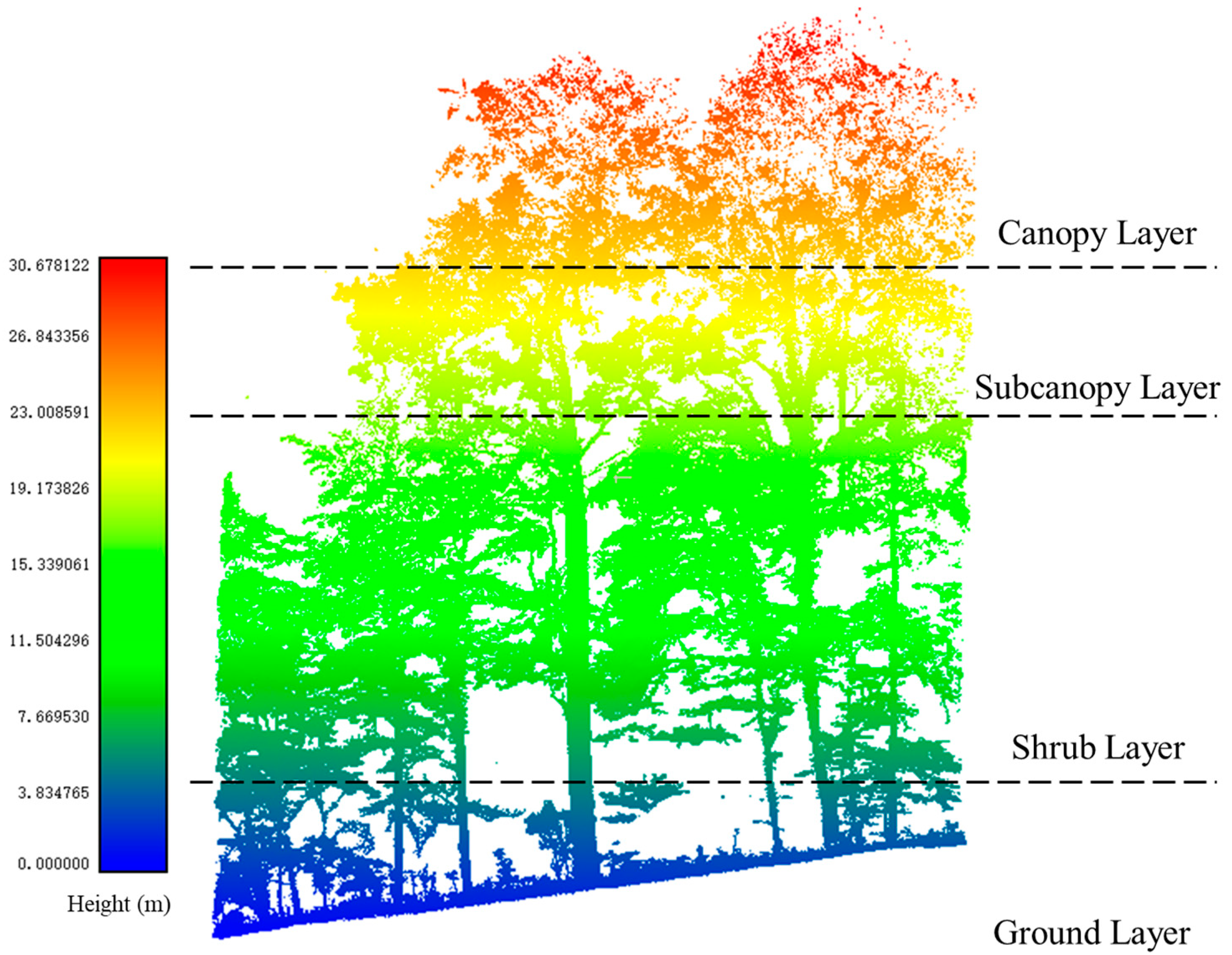
To better characterize the locations and significant errors in the separation results of the three plots, we referred to other methods of vertical stratification for forest plots [45]. In this study, the canopy structures of the forests in the point cloud data were categorized into canopy, subcanopy, shrub, and ground layers, as shown in Figure 5. These layers did not have clear demarcations and only represented approximate areas. The canopy mainly contained leaves, while there were fewer branches. In the subcanopy, the proportions of branches and leaves were comparable. As for the shrub layer, it had more branches.

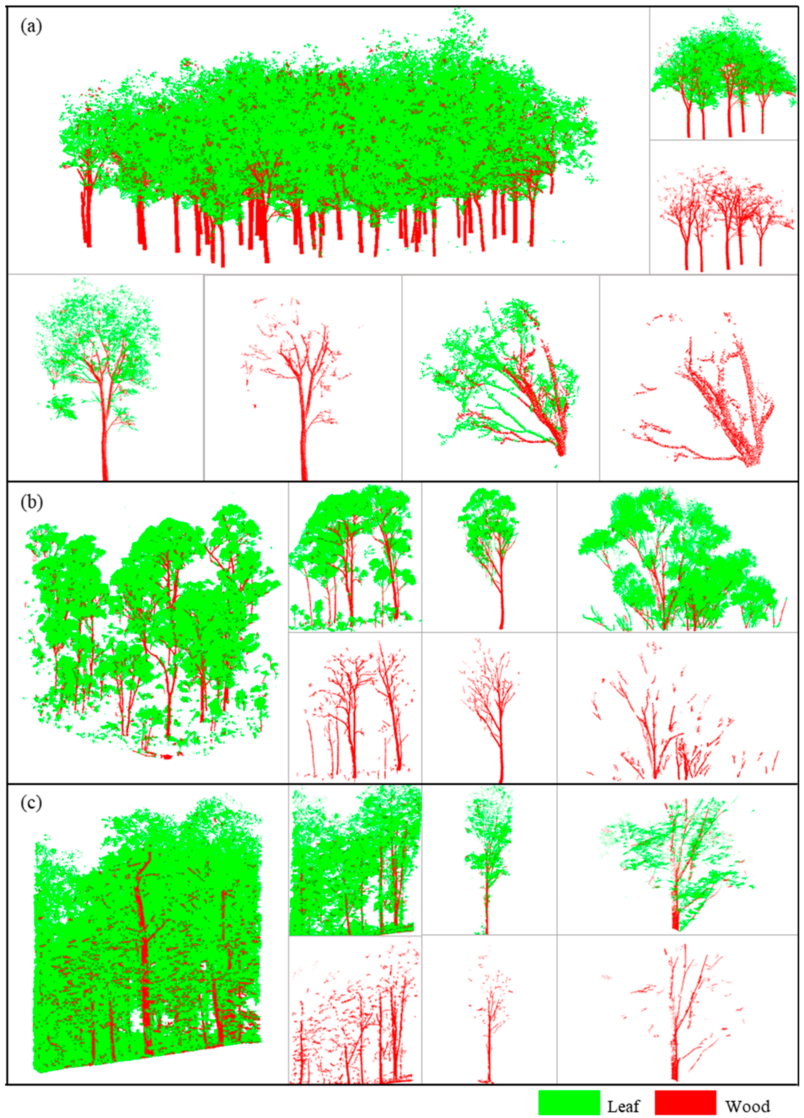
Figure 6a–c qualitatively represent the overall results and cropped sections of the final separation using the proposed method in the three sample plots. Red indicates separated wood, and the green indicates leaves in the figure. It can be seen that wood and leaves were successfully separated in the forest plots after processing with our method.

Figure 6a shows that leaves were mainly clustered in the canopy and subcanopy layers of the trees and were relatively neat in their growth in Plot 1. In this plot, the leaf distribution was relatively dense, and the method used in this study was more effective in separating the subcanopy layer. The main factor causing errors was the misclassification of leaves as wood in the canopy. As shown in Figure 6b, in Plot 2, leaves were primarily clustered in the canopy layer, while the bare branches in the subcanopy layer were distinct and could be extracted effectively. Due to the simple structures of the trees, it was easier to identify where errors occurred. Extracting wood from clusters with large numbers of overlapping leaves was challenging. In Plot 3, the structure was complex due to the fact that it was a natural forest with large numbers of leaves distributed in all layers. As can be seen in Figure 6c, the proposed method was accurate in identifying obvious wood, but many leaves were still misclassified as wood.

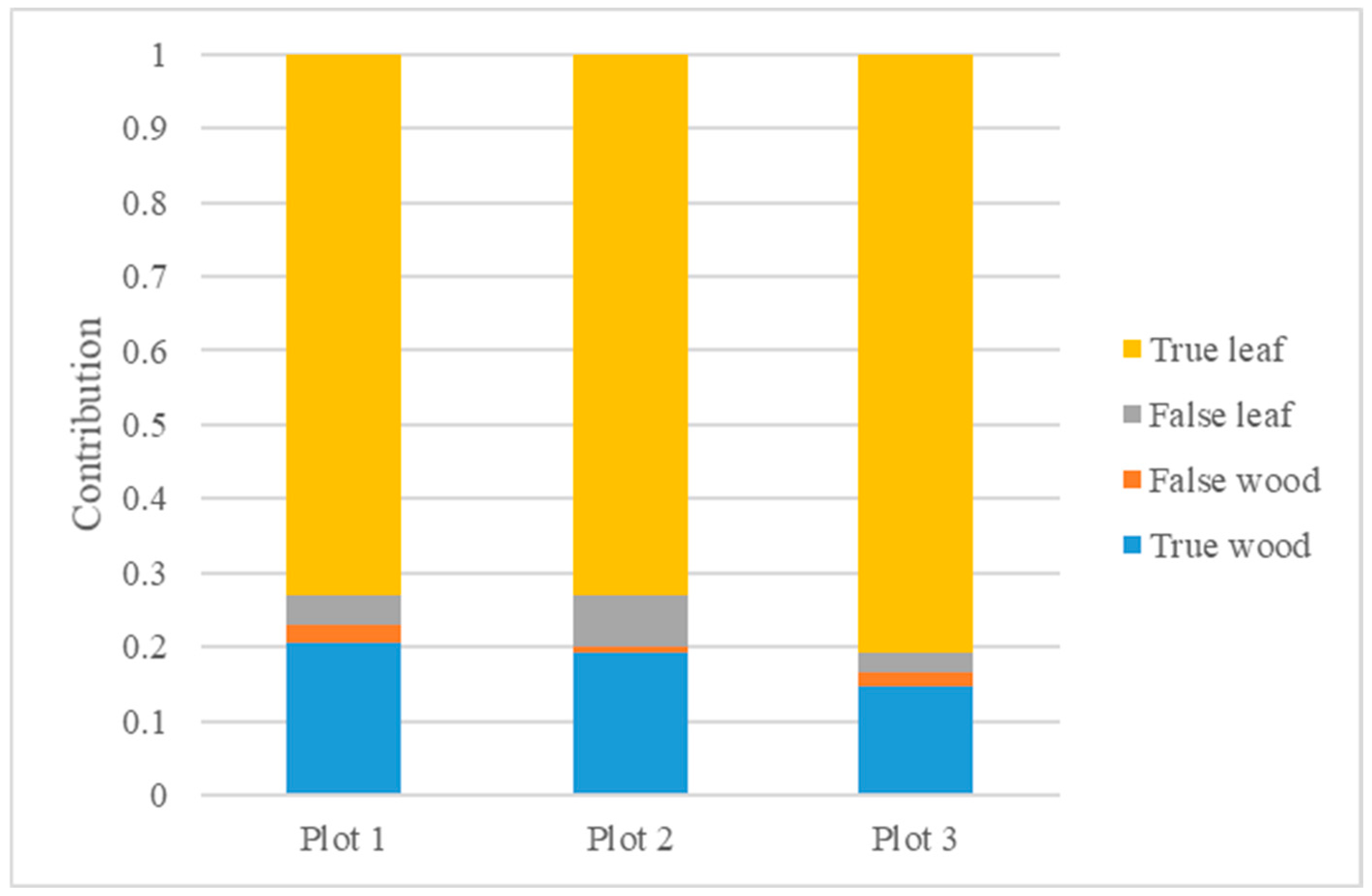
We used the experimental results and treated the manual segmentation as the reference for true separation. The results of the proposed method were compared with these manual results. The datasets were aligned, and the agreement at each point was checked. The numbers of points that were correctly or incorrectly categorized were then tallied accordingly. Figure 7 illustrates the contribution of each part, where a false leaf indicates a point where wood was incorrectly separated as a leaf. False wood is the opposite. It can be seen that the main cause of error was the misclassification of wood as leaves, in line with the response in Figure 6.

As can be seen in Figure 7, the point clouds of the three plots were dominated by leaves, ranging from 76% to 83%, and they contained relatively little wood. Therefore, when using the metrics for result assessment, clusters with larger leaf bases tended to show relatively high and less sensitive metrics for leaves, while the metrics for wood were more sensitive to errors.

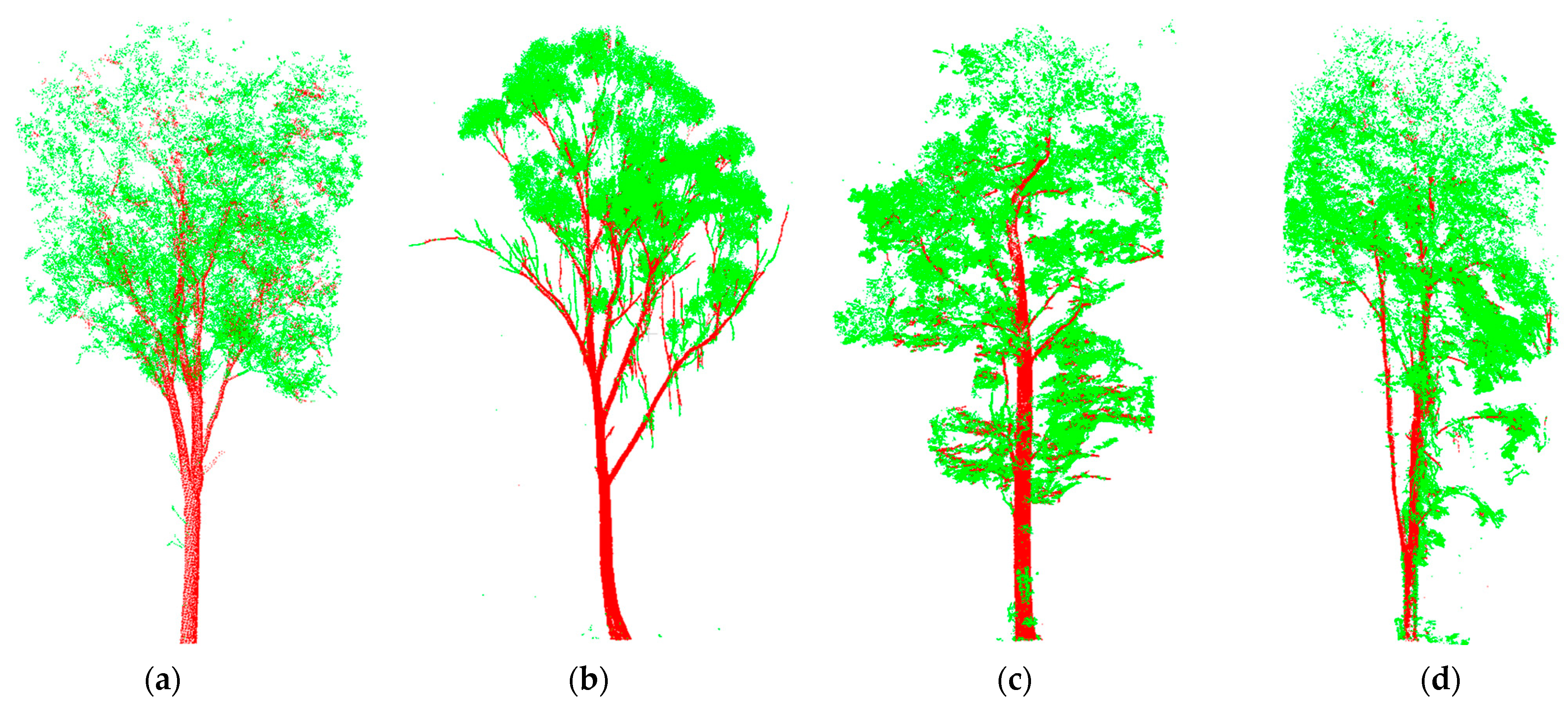
For the separation results of the different tree species, Figure 8 shows the separation of the individual trees within the plots. Figure 8a,b are from Plot 1 and Plot 2, respectively, while Figure 8c,d represent different tree species within Plot 3. Among these four main tree types, the canopy structures of (a) and (c) were more complex compared to (b). There were more types of tree species in Plot 3, with (c) and (d) being two representative types. The trees belonging to type (c) had many branches, similar to (a). Due to the complex canopy, canopy shading was relatively severe. In contrast, type (d) had more small branches, and the leaves were mainly distributed at the ends of the branches, similar to (b). This type of tree had a simpler canopy structure. Despite the significant differences in tree types and structures in this experiment, good separation results were still achieved. Additionally, this method effectively addressed, to some extent, the errors commonly caused by canopy shading. In the illustrated trees, the main errors were caused by the numerous small branches present in (b) and (d).

5. Discussion

5.1. Sensitivity Analysis

In order to investigate the suitability of the selection of ${\mathrm{d}}_{\mathrm{c}}$ thresholds using the method proposed in this study, we selected different threshold ranges in each plot for comparison. The results of an accuracy assessment using different threshold ranges are shown in

Table 2. Accuracy evaluation results for different threshold ranges.

	Threshold Range	Accuracy	Pr-Wood	Pr-Leaf	Re-Wood	Re-Leaf	F1-Wood	F1-Leaf
Plot 1	[0, 1.5]	0.856	0.995	0.841	0.414	0.999	0.595	0.913
	[0.5, 1.5]	0.937	0.894	0.950	0.843	0.968	0.868	0.959
	[0.5, 5]	0.863	0.931	0.853	0.473	0.989	0.628	0.916
Plot 2	[0, 1.5]	0.914	0.969	0.901	0.691	0.992	0.806	0.944
	[0.5, 1.5]	0.922	0.952	0.914	0.738	0.987	0.832	0.949
	[0.5, 5]	0.917	0.971	0.904	0.702	0.993	0.815	0.946
Plot 3	[0, 1.5]	0.934	0.891	0.941	0.711	0.982	0.791	0.961
	[0.5, 1.5]	0.953	0.884	0.967	0.841	0.977	0.864	0.972
	[0.5, 5]	0.933	0.972	0.928	0.633	0.996	0.767	0.961

.

We chose three threshold ranges for comparison ([0, 1.5], [0.5, 1.5], and [0.5, 5]). As can be seen in the results for the three plots in Table 2, the $\mathrm{Ac}$ of [0.5, 1.5] was the highest. This shows that for the overall wood–leaf separation results, a ${\mathrm{d}}_{\mathrm{c}}$ range of [0.5, 1.5] was selected for the most favorable results. Using [0.5, 1.5] as a base, when comparing the results with the other ranges, both the $\mathrm{Pr}\text{-}\mathrm{wood}$ and $\mathrm{Re}\text{-}\mathrm{leaf}$ were found to be lower. In contrast, the $\mathrm{Pr}\text{-}\mathrm{leaf}$ and $\mathrm{Re}\text{-}\mathrm{wood}$ were the highest in all three plots.

We can explain the above phenomenon with the help of Figure 4. We can approximate it in this way: The dc of case (a) in Figure 4 was mainly distributed in the range [0, 0.5], and similarly, cases (b) and (c) were distributed in [0.5, 1.5] and [1.5, +∞], respectively, as shown in Figure 4d. Thus, it can be seen that in choosing the range [0, 1.5], we misclassified a number of (a) categories as leaves. Similarly, in choosing the range [0.5, 5], we misclassified a number of (c) categories as leaves. That is, the proportion of leaves that were correctly identified in our results decreased in this case. The proportion of all real wood that was correctly identified using our method also decreased. This is why $\mathrm{Pr}\text{-}\mathrm{leaf}$ and $\mathrm{Re}\text{-}\mathrm{wood}$ decreased in both ranges.

It is worth noting that this dividing line was not absolutely correct, and there was some crossover between the three categories. Crossover was the main cause of error in the [0.5, 1.5] range. The crossover led to another phenomenon: Changing the threshold correctly categorized all leaves in these crossed ranges in (b). That is, the proportion of wood that was correctly identified increased in this case. The proportion of all real leaves that were correctly identified also increased. This led to increases in $\mathrm{Pr}\text{-}\mathrm{wood}$ and $\mathrm{Re}\text{-}\mathrm{leaf}$ in the ranges [0, 1.5] and [0.5, 5].

As described above, different accuracy metrics increased or decreased when different threshold ranges were selected. Due to the crossover of the ${\mathrm{d}}_{\mathrm{c}}$ ranges in several cases, it was difficult to find a threshold range where all accuracy metrics were superior. As demonstrated by $\mathrm{F}1\text{-}\mathrm{wood}$ and $\mathrm{F}1\text{-}\mathrm{Leaf}$ in Table 2, after balancing the effects of both $\mathrm{Pr}$ and $\mathrm{Re}$, the threshold range [0.5, 1.5] was clearly advantageous. Therefore, the ${\mathrm{d}}_{\mathrm{c}}$ range of [0.5, 1.5] was chosen for the evaluation of the results and comparison with other methods in this study.

5.2. Accuracy Validation and Method Comparison

We compared the method proposed in this study with the widely used LeWoS proposed by Wang et al. [46]. LeWoS used the default parameters in this experiment because it had fewer adjustable parameters and satisfactory robustness. The proposed method was also compared with a supervised learning method based on a Random Forest model (RF model) proposed by S. M. Krishna Moorthy et al. [26]. The model was trained by the authors using five plots located at two different locations and two single trees. They could be separated using the authors’ trained model directly. The model was compared to a number of other state-of-the-art methods described in the literature and could represent most machine learning models.

The results for the quantitative evaluation metrics for our method and the methods used for comparison (LeWoS and the RF model) are shown in Figure 9. For our method, the $\mathrm{Ac}$ of the three plots was higher than 0.9. $\mathrm{Pr}\text{-}\mathrm{wood}$ was approximately 0.92 ± 0.03. $\mathrm{Pr}\text{-}\mathrm{leaf}$ was approximately 0.94 ± 0.03. $\mathrm{Re}\text{-}\mathrm{wood}$ was approximately 0.79 ± 0.05. $\mathrm{Re}\text{-}\mathrm{leaf}$ was 0.97. $\mathrm{F}1\text{-}\mathrm{wood}$ and $\mathrm{F}1\text{-}\mathrm{Leaf}$ were 0.84 ± 0.02 and 0.96 ± 0.01, respectively. The lowest $\mathrm{F}1\text{-}\mathrm{wood}$ was in Plot 2, which also reached 0.83, indicating the high accuracy of our method.

In comparison to LeWoS, our method had more metrics that were superior. Figure 9a,c show that our method was significantly superior to LeWoS in the processing of Plots 1 and 3. While Figure 9b shows that our method had some metrics that were superior to LeWoS in Plot 2, several metrics were lower. Overall, it was about on par with LeWoS. This was also true when compared to the RF model. Our method was significantly superior to the RF model for both $\mathrm{Pr}\text{-}\mathrm{wood}$ and $\mathrm{Re}\text{-}\mathrm{leaf}$ in the three plots. This indicates that our method is significantly more accurate in detecting wood than the RF model when confronted with different forest types. In the three plots, the RF model showed a greater degree of uncertainty, with drastic changes in accuracy.

In Plots 1 and 3, the accuracy of our method was significantly higher than those of LeWoS and the RF model due to the complex canopy structures of these two plots. This phenomenon indicates that our method addressed the problem of difficult segregation in complex forests to a certain extent. Meanwhile, for Plot 2, which had a relatively simple canopy structure, our method was better than LeWoS for several metrics, and the overall accuracy was basically the same. Although the RF model’s $\mathrm{Re}\text{-}\mathrm{leaf}$ was significantly better than those of the other two methods in Plot 2, its Pr-wood was undeniably lower, which led to its $\mathrm{F}1\text{-}\mathrm{wood}$ and $\mathrm{F}1\text{-}\mathrm{leaf}$ values being lower than those of the other methods. Overall, the $\mathrm{Re}\text{-}\mathrm{wood}$ of our method was relatively low in all three plots. This was consistent with the contributions. It also further suggested that $\mathrm{F}1\text{-}\mathrm{wood}$ was less accurate in the three plots compared to the other metrics.

Among the three plots, the $\mathrm{Pr}\text{-}\mathrm{wood}$ and $\mathrm{Fa}\text{-}\mathrm{wood}$ of our method were significantly better than those of LeWoS and the RF model. This indicates that the correct proportion of the predicted wood was relatively high with our method. That is, the problem of classifying a large number of leaves as wood was addressed to a certain extent. The $\mathrm{Re}\text{-}\mathrm{wood}$ of our method was higher in Plots 1 and 3 but lower in Plot 2. This shows that for a simple canopy structure, the LeWoS treatment was superior, but our method found wood easier in a complex structure. On the other hand, while the RF model performed better in simpler canopy structures, it still had lower performance compared to LeWoS.

The better accuracy of our method was mainly due to the point cloud clustering described in Section 3.2. Our method divided the points into clusters with only leaves or wood, which made them easier to detect (Figure 3). The combination of the above caused the $\mathrm{F}1\text{-}\mathrm{wood}$ values of Plots 1 and 3 to be significantly higher than those of LeWoS and the RF model, while these values were the same in Plot 2. For leaves, the accuracy values of all methods were high for all indexes, which was due to the large base of leaves; that is, the proportion of leaves in the point cloud was relatively high (Figure 7).

5.3. Uncertainty Analysis

The cluster-based method proposed in this study showed effectiveness in three different plots. Through the detailed qualitative and quantitative results, it was shown that this method can achieve efficient and highly accurate wood–leaf separation in actual scenarios. In these plots, the proposed method effectively handled differences in geographical locations, tree species, and point cloud densities, indicating its versatility and robustness in diverse environments.

Specifically, detailed zoomed-in views are shown in Figure 6 and Figure 10. In Figure 10, the (2) in each figure represents a region with a relatively good separation effect. As can be seen in the figure, the proposed method also extracted relatively coarse wood well and was less affected by sheltering. Quantitatively,

Table 3. Comparison between plot parameters and accuracy of separation results.

	Point Density (Points/m2)	LAI	Canopy Cover	Accuracy	Pr-Wood	Pr-Leaf	Re-Wood	Re-Leaf	F1-Wood	F1-Leaf
Plot 1	24,413	4.57	0.767	0.937	0.894	0.950	0.842	0.967	0.867	0.958
Plot 2	4934	1.438	0.272	0.922	0.952	0.914	0.737	0.986	0.831	0.949
Plot 3	18,366	9.49	0.964	0.953	0.883	0.967	0.840	0.976	0.863	0.971

shows a comparison between the plot parameters and the accuracy of the separation results. Table 3 illustrates that the proposed method showed strong robustness in the face of different parameters, such as the point density, the LAI, and so on.

However, some points were still misclassified. The occurrence of such situations can be attributed to two main factors. On the one hand, errors might have arisen during the initial clustering step, where some leaf points were mistakenly clustered with wood points. Additionally, for very thin wood, which sometimes comprised only a single row of points, accurately clustering it with other wood was challenging, leading to separation difficulties during the subsequent extraction. Figure 10 shows the local areas of the point cloud data that exhibited the above characteristics. On the other hand, setting the Chaos Distance threshold could have introduced errors because it had to be adjusted based on the specific characteristics of the plots. As mentioned in Section 5.1 and shown in the lower part of Figure 4, the dividing line between leaf and wood was not clear when choosing the Chaos Distance threshold range. Inaccurate threshold settings might have led to deviations or errors in the separation process.

Other factors might have contributed to the observed situations. One such factor is the inherent complexity and variability of the natural environment. The data might have contained inherent noise, occlusions, or irregularities caused by vegetation density, lighting conditions, and sensor limitations. These factors might have introduced uncertainties and made it challenging to separate wood and leaves accurately.

Therefore, the combination of these factors, including the inherent challenges posed by clustering and the sensitivity of the parameter settings, contributed to inaccuracies in the wood–leaf separation process.

5.4. Efficiency Comparison and Analysis

In terms of the efficiency of the algorithm, the method had a time complexity of $\mathrm{O}\left(\mathrm{n}\log \mathrm{n}\right)$, where n is the total number of points in the point cloud. The actual execution duration varied depending on the size of the point cloud data and the specific parameters used for clustering and classification. C++ was the programming language used to implement the wood–leaf separation algorithm proposed in this study. The primary third-party library was the Point Cloud Library (PCL) [31]. The specific implementation algorithm was compiled using the Microsoft Visual Studio Community 2022 development environment. The open-source algorithm LeWoS, which was used for comparison, was run on the same computer using MATLAB Runtime [3]. The RF model algorithm used for the comparison was run using the Python 3.7 environment with version 0.21.3 of the scikit-learn library. The operating system was Windows 11 Professional Edition 22H2. The processor was an eleventh-generation Intel Core i5-11400H @ 2.70 GHz with 16.0 GB of RAM. Due to the large amount of data, which could easily exceed the computer’s memory, we opened an additional 30 GB of virtual memory (this was to “pretend” that a part of the hard disk space was for memory use, and the disadvantage was that this part of the space was slower to read and write). The recorded plot processing times of our method, LeWoS, and the RF model are shown in

Table 4. Comparison of processing times for sample plots.

	Number of Points	Time Cost (min)
		Our Method	LeWoS	RF Model
Plot 1	5,042,403	5.18	8.87	313.37
Plot 2	6,388,675	3.75	10.73	223.37
Plot 3	8,833,993	14.52	20.4	1523.3
Average	6,755,024	7.82	13.33	686.68

, which indicates the processing durations for the three study plots. The average processing duration was 7.82 min. It should be noted that the processing times for all methods are the times required to process the preprocessed data. All three methods used the same preprocessing method, as described in Section 3.1.

Compared with LeWoS and the RF model, the proposed method demonstrated significantly better performance when processing the same data. The main time consumption of the proposed method occurred during the estimation of the point cloud normal vectors and the regional growth clustering process, which was evidently related to the amount of data. The running time of the method in this study was directly related to the number of points in the point cloud and the number of clusters after clustering. The number of clusters was related to the characteristics of the data and the parameter settings used for clustering (such as the smoothing threshold, curvature threshold, the number of search points, etc.). Specifically, the focus was on the need to obtain point cloud neighbor information during normal vector estimation for point cloud clustering. This made it necessary to perform a traversal process on the entire point cloud. When clustering, different parameters, such as smoothing thresholds, curvature thresholds, the number of search points, etc., can lead to large differences in the cluster size, the degree of smoothing, and other characteristics. These differences may lead to significant time costs, such as variations in the frequency of updating seed points due to different parameter settings. In the subsequent separation process, in order to increase the efficiency of the algorithm, we first performed a preliminary separation of the wood in the clustering results. This effectively extracted the wood clusters that contained more points. In the final separation, we were only faced with the remaining clusters, which contained fewer points. The traversal of these clusters could be carried out efficiently to achieve the final separation. In addition, another reason why our approach was more effective than LeWoS and the RF model could be the choice of programming language. It has been shown that C/C++ is significantly more efficient than other languages in terms of runtime [47].

For the three plots in the experiment, the main reason why the time for Plot 2 was shorter than that of Plot 1 was that the proportion of ground points in Plot 2 was relatively low. After removing the ground points, there were 2,820,945 points left in Plot 2 and 3,270,721 points left in Plot 1. In addition, as shown in Figure 6, in Plot 2, the trees had a simpler structure compared to Plot 1, where the trees had more branchlets and leaves. This made the algorithm take more time to perform clustering in Plot 1, and it produced more clusters. The processing time for Plot 3 was significantly longer than for the other two plots. This was partly because the proportion of ground points in the data was smaller and because the number of points was significantly higher. Additionally, the structure of the canopy in Plot 3 was complex, with more intersections between trees and a high proportion of leaves. This resulted in more clusters, which further increased the run time.

6. Conclusions

In this study, we proposed a method based on cluster features for separating leaves and wood in forest plots using terrestrial LiDAR point cloud data. The main idea behind this method is to leverage the morphological differences between wood and leaves for separation. A point cloud with nonground points is clustered into groups using a region-growing clustering algorithm. Preliminary wood separation is then performed based on the cluster size and the number of points. Subsequently, the final wood extraction is completed by combining the Chaos Distance, and finally, the separation accuracy of the wood–leaf separation is verified. The proposed method is simple to implement. The Chaos Distances proposed in this study demonstrated high accuracy and efficiency, with an average recall rate of 0.89 and an average precision of 0.92. This validated the effectiveness of separating wood from leaves in forest plots. The study plots had an average of 44 trees, and all plots were treated with high efficiency. In addition, this method had good effects on different tree species and forest areas. The method comparison results show that the proposed method has higher accuracy in complex canopy structures and dense forests. Future work could focus on integrating this method with other remote sensing technologies, which could enhance its application in large-scale forest monitoring and management.