Abstract
Soil nutrient content varies spatially across agricultural fields in hard-to-predict ways, particularly in floodplains with complex fluvial depositional history. Satellite reflectance data from the Sentinel-2 (S2) mission provides spatially continuous land reflectance data that can aid model development when used with point observations of nutrients. Reflectance from vegetation is assumed to obstruct land reflectance of bare soil, such that researchers have masked vegetation in models. We developed a routine for masking vegetation within Google Earth Engine (GEE) using Random Forest classification for iterative application to libraries of S2-images. Using gradient boosting, we then developed soil nutrient models for surface soils at a 250-ha agricultural site using S2 images. Soils were sampled at 2145 point locations to a 23-cm depth and analyzed for Ca, K, Mg, P, pH, S, and Zn. Results showed that masking vegetation improved model performance for models from subsets of the data (80% of samples used for model development, 20% validation), but full data sets did not require masking to achieve accuracy. Models of Ca, K, Mg, and S were successful (validation R2 > 0.60 to 0.96), but models for pH, P, and Zn failed. Bare soil composite images from S2 data are helpful in predicting soil fertility in low-relief floodplains.
1. Introduction
Soil fertility is important for plants, including crops, and for supporting biological systems in general because crops and terrestrial organisms depend on nutrients that can be found in various quantities in the soil matrix [1]. Soil fertility varies spatially, even within homogenously managed agricultural fields, because of soil physical, chemical, and geological conditions [1,2,3,4]. Detailed soil fertility maps are desirable for effective soil management but are challenging to produce due to the high spatial and temporal variability of soil fertility factors (soil organic matter, mineralogy, plant-available nutrients, etc.), the high costs of soil sample extraction and laboratory analysis for control points, and the often unknown extent to which a limited set of samples can be relied upon to represent contiguous non-sampled soil areas [5,6,7].
Soils in floodplains are spatially complex owing to complex fluvial dynamics that can cause abrupt shifts in soil parent material, texture, and mineralogy even within topographically homogenous, flat landform profiles that show little apparent variability. Such landscapes are often rife with marks from archaic stream meanders and sporadic flood episodes that have deposited heterogeneous material over geologic time [5,8,9]. Land-surface reflectance of electromagnetic radiation is useful in the study of soil spatial and geographic variability [8,10,11,12,13,14,15,16,17,18] and is particularly salient in situations where variability may be unexpectedly high, such as in floodplains [5,9]. In such landscapes, where soil heterogeneity is high, spatial and temporal land-surface reflectance variability can indicate areas of soil variability that are not otherwise obvious [17]. Satellite reflectance data are sensitive both directly and indirectly to several properties related to soil fertility, including organic matter content, moisture content, soil mineralogy, soil depth, and soil texture [10,11,12,17,19,20]. For example, soil organic matter (SOM) is dark, causing soils with higher levels of SOM to have a lower albedo and reflect electromagnetic energy to a lesser extent than soils with lower SOM levels [13]. In turn, soils higher in SOM often have higher concentrations of nutrients. This and other relationships between soil properties and reflectance, such as the effect of soil moisture content in decreasing a soil’s albedo [21], may allow the use of reflectance data to explain the spatial distribution of nutrient contents in soils.
Complicating the interpretation of the signal measured by satellite reflectance from the soil are the variable effects of vegetation, both living and in the form of plant residues [13]. Importantly, plant communities cycle nutrients near the soil surface where they can be more readily available to growing plants, but they also block direct reflectance information from the soil surface [1,14,19]. In one sense, reflectance data from vegetation represents a response to environmental and soil conditions and can provide some indirect information about soil fertility. Where vegetation thrives, it can be inferred that conditions are adequate with respect to soil nutrition. On the other hand, vegetation blocks direct reflectance from bare soil to the satellite sensor and represents a modification of any direct signal from soil components. While the presence of vegetation in an image does not necessarily preclude its use in predictive models, relationships between land reflectance and soil properties are believed to be stronger when bare soil images are used [5,11]. This is because vegetation and crop residues can interfere with information gained about soil properties from reflectance images [13,14]. Conversely, analysis of bare soil may elucidate the most reliable relationships between soil fertility and reflectance because electromagnetic radiation reflected from bare soil gives information about the interaction of radiation with the components of soil with minimal interference. Vegetation obscures reflectance from the soil by covering it and can give a misleading uniformity of reflectance in a field of a single crop with uniform growth, obscuring soil variability. Vegetation can also show variability not pertaining to soil but rather to differences in planting rates, variations in crop choice, or other factors. Furthermore, different vegetation types may have different reflectance characteristics not directly related to soil characteristics. Also, differences in land use can be independent of soil characteristics but nevertheless display marked differences in reflectance.
For these reasons, several researchers have made attempts to remove the vegetation signal from reflectance data of serial imagery, preferentially retaining bare soil information when possible [8,15,16]. Given the relative scarcity of images depicting bare soil, particularly in humid locations where vegetative cover is consistent throughout growing seasons, many scenes may be needed for this approach. The scarcity of images results from humid areas having crop cover, crop residue, snow, or perennial vegetation cover for much of the year. Short windows of cultivation during planting seasons can sometimes offer glimpses of bare soil reflectance characteristics. Some authors used a W-Net approach to discriminate bare soil from other reflectance data, using thresholds of vegetation and wetness indices to mask features that are not bare soil [18]. Several authors mapped SOM during a bare soil period but only used one Sentinel-2 (S2) scene acquired when soils were sampled [22]. The use of time-series satellite data where satellite revisit times permit multiple collections of reflectance data within a single season or year has the advantage that they potentially show dynamic interactions among features such as precipitation, vegetation, soil moisture variability, and soil properties [8,16].
To our knowledge, no research has yet used machine learning supervised classification to automate vegetation masking applied to all available images in an S2 satellite collection to extract bare soil pixels for environmental correlation with soil properties. The objectives of the current study were to (1) determine the importance of remote sensing satellite reflectance data as an environmental covariate in predictive soil mapping of Ca, K, Mg, P, pH, S, and Zn in an agricultural floodplain, (2) develop a machine learning methodology using Google Earth Engine (GEE) for removing the potentially obstructive influence of vegetative pixels, thereby maximizing the information available from a suite of satellite images available for analysis, (3) determine whether pixel-based statistics from spectral data from satellites could be used to estimate soil fertility properties at the site, (4) use machine learning to train artificial intelligence to recognize and classify bare-soil portions of images that could then be analyzed for relationships between bare soil reflectance and soil fertility in the surface, and (5) make models of soil fertility properties for the site and assess them for accuracy. A further objective was to assess the accuracy of soil fertility predictions with and without the automated vegetative masking of images, thereby assessing the usefulness of the vegetation masking technique. To test our new vegetated pixel masking tool, we sought to determine the strength of relationships between soil fertility and reflectance scenes by generating a histogram-based gradient boosting interpolation routine to predict surface Mg, Ca, K, P, S, Zn, and pH in an agricultural area with extensive soil sample density (2145 point-locations). This research should be useful for efforts to generate high-detail, high-resolution geospatial maps of soil fertility properties in floodplains with intermittent vegetation cover.
2. Materials and Methods
2.1. Study Area
The study was conducted in Washington County, in Western Mississippi, USA, at the National Center for Alluvial Aquifer Research in the Mississippi Alluvial Plain. The site is approximately 250 hectares (2.5 km2) (Figure 1), with a mean elevation of approximately 37 m. Elevation is highest at the north end near Deer Creek and decreases only about three meters to the southern end of the site, nearly three kilometers away, in a slow, gradual declension with an average slope of approximately 0.1%. Following the pattern of gradual decrease in elevation, coarse sediments near Dear Creek overlie a thicker clay-rich layer of the broader floodplain, with the coarser levee deposit thinning out towards the south as the elevation decreases [9]. Texture grades from very fine sandy loam soils at the north (Bosket series, a fine-loamy, mixed, active, thermic Mollic Hapludalfs) to clay at the south (Downling, a very-fine, smectitic, nonacid, thermic Vertic Endoaquepts), and Sharkey (a very-fine, smectitic, thermic Chromic Epiaquerts) [23].
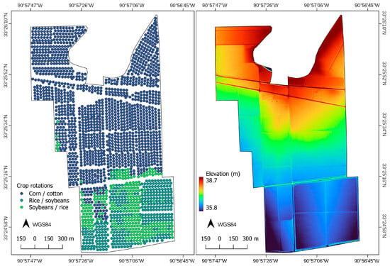
Figure 1.
Soil sample locations and crop rotations (left) and elevation model of the study site (right). The site is in Washington County, Western Mississippi, USA.
The site has a long history of row cropping with corn (Zea mays), cotton (Gossypium spp.), rice (Oryza sativa), and soybeans (Glycine max). Because the soils in the northern portions of the site are better drained, they have historically been cropped with alternating rotations of corn and cotton, while the southern portions of the site, marked by the higher clay soils of Sharkey and Downling, have been cropped with alternating rice and soybean rotations (Figure 1).
2.2. Soil Sampling and Laboratory Analysis
Soils were collected at 2145 point locations at the study site, approximately one sample for every 0.13 ha (i.e., approximately 9 samples per hectare). For each point location, soil from a sampling depth of 0–23 cm from the surface was aggregated, passed through a 2-mm sieve, and air-dried. To measure pH, a portion of each sample was then diluted with water to a 1:2 soil-to-water ratio and evaluated with a calibrated glass electrode. Soil nutrients Ca, K, Mg, P, S, and Zn were evaluated by extraction with the Mehlich-3 extract methods using a 1:10 soil mass:extractant solution volume ratio and analyzed by inductively coupled argon-plasma spectrometry (ICP, Agilent Technologies, Santa Clara, CA, USA) [24,25].
2.3. Data Analysis and Model Development
The analysis of soil, reflectance, and elevation data and development of soil nutrient models was conducted using R and packages tidyverse, caret, terra, sp, sf, clhs, ggpointdensity, and sen2r [26,27,28,29,30,31,32,33,34,35]. Development of the model to acquire S2 satellite reflectance data and to identify and mask vegetation from images was done using Python 3.12 and GEE [36].
2.3.1. Geospatial Data
We used a 1-m resolution digital elevation model made with laser altimetry for the site in Western Mississippi from the United States Geological Survey 3DEP program as a base map [37]. Elevation data were acquired between 24 January 2019 and 29 February 2019 using the Riegl 1560i system capable of acquiring 1.3 million measurements per second mounted on a Piper Navajo twin-engine aircraft [38]. The average point spacing was 2.04 points m−2 [38]. Light-detection and ranging (LiDAR, or airborne laser altimetry) bare-earth returns were converted to 1-m elevation rasters through a proprietary linear interpolation algorithm applied to a triangulated irregular network with a required vertical accuracy of 0.196 m [37]. These DEM data were made freely available to the public through the USGS website [39].
Reflectance data collected by the MultiSpectral instrument aboard the Sentinel-2A and B satellites of the Copernicus Mission of the European Space Agency [40] were used as input data for the soil fertility models for several reasons. Features such as the wide availability of these data through GEE from 2017 to the present, free and public open access, high spatial resolution 10-m pixels for most bands of the sensor, and high temporal resolution with a 5-day revisit time, made this dataset practical and useful for geospatial modeling purposes [5].
Cloud removal was accomplished programmatically through the cloud probability dataset contained in the Earth Engine Data Catalog, which offers the probability of pixels being cloud. Probabilities in this dataset were calculated by the s2cloudless Python package, which uses a tree-based algorithm (LightGBM) [41] trained with S2 bands to infer cloud probabilities. Pixels with greater than 80% probability of being cloud were computed as non-data for all utilized S2 images.
Some authors developed a methodology for collecting a bare soil mosaic from Landsat images to produce an unfragmented spatially continuous surface, or composite, which could represent unobstructed soil reflectance [15]. Their hypothesis was that the soil surface of their area of interest had been exposed to satellite measurements at least once, and each occurrence from multiple images could be aggregated into a single representation. They used thresholds of univariate spectral indices calculated from mutable band reflectance, including the normalized difference vegetation index (NDVI) to distinguish vegetation from bare soil and the normalized burn ratio 2 (NBR2) to distinguish areas showing influences of straw lignin, burned vegetation, and cellulose from bare soil. All areas flagged as clouds, cloud shadows, vegetation, water, or 6 provisional thresholds of the NBR2 were classed as non-data. The remaining pixels for all available images were summarized by selecting the median value of each pixel from all images for each spatial grid cell, thereby producing the bare-soil composite image. This bare-soil composite image was then used as an environmental covariate to predict soil properties and compared to a set of measured ground truth data. A similar effort was made by other authors to create a bare-soil composite using Landsat-4 through Landsat-8 images from 1985–2017 [42]. These authors aggregated the data to provide a pixel-by-pixel analysis that returned, for each pixel, the most representative instance of a bare pixel according to thresholds established to characterize a bare soil index (BSI) value. Pixels with the best BSI scores were returned as values in the final output images. Models for soil properties of SOM, clay, silt, and sand were then created using the BSI pixel image and multiple linear regression.
The vegetation masking algorithm was developed for this project in GEE using 10,531 hand-labeled data points on nine scenes for training the model. The selection of the training set prioritized scenes distributed throughout the year and containing representative pixels of crops and bare soil. The training set comprised scenes from January, March, April, and October of 2019; February, March, August, and October of 2020; and November 2021. To train the machine learning algorithm to distinguish bare-soil parts of images from vegetated parts of images, it was necessary to choose images that contained pixels depicting both bare soil and vegetated areas. It was assumed that these 9 scenes would provide sufficient training and testing opportunities for developing a classifier and testing it with independent samples. About half of the points were classed by human operators as bare soil (n = 5448) and half were classed as vegetation (n = 5083). Further, 80% of these hand-labeled points were used to train the model, and 20% were retained as validation points for assessing the accuracy of the model.
The Random Forest algorithm implemented within the GEE API was then trained on the 80% training data sampled from the nine training scenes and was applied to the entire available catalog of S2 images for the site. The intent of the model was to predict vegetated pixels of any image within the S2 image catalog and use this classification as a mask for removing vegetated pixels from each available scene, thereby providing scenes with only bare soil pixels for further analysis. In our analysis, we only included scenes from the cropping seasons (between June and October, from 2019 to 2023). The intent was to examine the influence of growing vegetation on the performance of models predicting soil fertility and to compare vegetated scenes to bare soil scenes. Since the presence of vegetation is minimal for much of the year in the studied site, summary statistics of all the scenes for all months do not capture the effects of vegetation very well. For this reason and also to simulate the case where bare soil scenes are hard to obtain, we chose to limit our time span to the five cropping seasons from June to October, during the years 2019–2023.
Vegetation masking was applied to the time series of images in the following way. First, each pixel of each time-series image was classified as vegetated or not vegetated following the vegetation masking algorithm described above. Two datasets were then analyzed separately, those with vegetation pixels masked (masked imagery) and those without any modification to the images (not-masked). Every pixel classed as vegetation was flagged as non-data and removed from the ‘masked’ dataset, but retained in the ‘not-masked’ dataset (Figure 2). The first dataset consisted of composites representing the median and interquartile ranges (IQR) calculated without masking vegetation (not-masked) for the analyzed period (between June and October, from 2019 to 2023). Next, composites were created to represent the median and IQR using vegetation-free pixels (masked) for the analyzed period. Composites were created for bands 2, 3, 4, 5, 6, 7, 8, 11, and 12. Other Sentinel-2 bands, such as bands 1, 9, and 10, were not used because they were assumed not to be relevant to terrestrial analysis of vegetation and bare soil characteristics. Band 1, for instance, gives information relevant to coastal aerosols; band 9 gives information about water vapor; and band 10 gives information about cirrus clouds. Thus, 18 images were produced for each dataset, 9 representing median pixel values for each pixel, and 9 representing the IQR of values from the time series for each pixel. Thus, 36 images were produced without masking vegetation (n = 18) and with vegetation masking (n = 18), representing statistical summaries of the reflectance characteristics of the study site. The median composite images were calculated to represent the central tendency in the time series of the reflectance values, while the IQR composites were intended to capture the range of variability in reflectance over time. IQR was chosen over standard deviation because we believed it would be less susceptible to extreme values. The calculation of the median value was likewise preferred as a measure of central tendency over the mean because it would be less susceptible to extreme values. The difference in values of IQR and mean reflectance are discussed in greater detail in the results section, but briefly, it can be noted here, that pixels depicting vegetation have lower reflectance in the visible part of the spectrum and higher reflectance in the infrared and near-infrared parts of the spectrum. The intensity of reflectance values statistically summarized in the pixel statistics of the ‘masked’ vs. ‘not-masked’ datasets illustrate the differences due to vegetation removal.
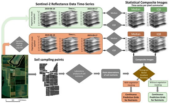
Figure 2.
Modeling process for developing soil nutrient models from point observations and satellite reflectance data from the S2 image. Arrows represent processing flow. Sampling points were collected and analyzed with Mehlich-3 extractant and ICP. Time-series images were collected and summarized for interquartile range and median values over time for each pixel in the image. The summaries were collected for each available band of the S2 library during the time period of the study. Output continuous prediction grids for soil nutrients were produced from the S2 data and point data with histogram-based gradient boosting both with and without vegetation masking. The site is in Washington County, Western Mississippi.
2.3.2. Model Development and Assessment
We used a histogram-based gradient boosting model with soil fertility response variables and statistical summaries of S2 surface reflectance as predictor variables [43]. To build soil nutrient maps, point samples were split into training and test sets (80/20%). Nutrient models were tuned by 10-fold cross-validations (CV) repeated 1000 times and tested against the test sets. CV was performed in the training set while varying the learning rate parameter. The learning rate has the purpose of decreasing the rate with which the model fits the data. Gradient boosting is a tree-based algorithm that creates many shallow decision trees (weak learners) sequentially. Each tree in the sequence tries to minimize the residuals of previous trees. Because trees know of the errors committed by their predecessors, they fit the data quickly and easily overfit. The learning rate thus constrains the rate of residual correction so that trees learn meaningful rules instead of convenient, unrealistic ones.
The goodness of fit was assessed using the coefficient of determination (R2) and the root mean square error (RMSE). The best-fit models were then tested against the validation set to identify possible overfitting. Importance scores of band statistics were calculated using permutation importance. Performance scores from permutation tests were calculated using the test set (the 20% split unseen by models). Permutation consists of shuffling the values of one of the variables (thus making the variable meaningless) and then calculating the validation score again (R2). The metric in the x-axis is the decrease in R2 after shuffling each variable 1000 times. Since several response variables were found to have similar spatial distributions, the most important variables selected by the algorithm for soil attributes were combined and used as explanatory variables for all response variables.
The effects of masking vegetation in prediction performance were also tested while varying sample density. The goal was to understand if the presence of vegetation affected prediction performance and if the effect was dependent on the number of samples used to train the spatial prediction model. Tests were performed for two sets of bands: visible (B2, B3, and B4), which were found less correlated to response variables, and infrared (B11 and B12), found to be more correlated to response variables, so to investigate the effects of vegetation masking in different parts of the spectrum. This evaluation was done by selecting n samples to train models and validating the model with all the remaining samples (2145 − n). One hundred repetitions were done for each model. First, results were compared for models trained based on masked and not-masked scenes using only the median of the tested bands. Next, IQR bands were added to test whether the results would improve.
3. Results
Soil fertility measurements of the 2145 soil samples taken from the soil surface of the 250-hectare study site are statistically summarized in Table 1. With only a few exceptions among the samples, values for pH and concentrations of P, Mg, Ca, and Zn were well within the tolerable range for conditions for agronomic crops [1] (Table 1). Concentrations of S and K, on the other hand, showed potential for deficiencies in some sample locations and the need for nutrient management strategies to correct nutrient imbalances [1]. Histograms of the measured soil nutrients are given in the Supplemental Materials (Figure S1).

Table 1.
Statistical summary of soil nutrient content extracted with Mehlich-3 extractant for surface soil samples (0–23 cm) at 2145 locations within the 250-hectare study site in Western Mississippi.
Data from the time-series imagery from the S2 mission for the study site is given in Table 2 for both original images and those that have had vegetation masking, removing pixels depicting vegetation by means of the masking algorithm. S2 reflectance imagery without vegetation masking had lower mean reflectance values for bands 2, 3, 4, 5, 11, and 12 than imagery with vegetation masked (Table 2). Bands 6, 7, and 8, however, showed stronger reflectance values in the images without vegetation masking, indicating the strong tendency of vegetation to reflect light in the near-infrared part of the spectrum while absorbing light in the visible part of the spectrum. In all bands except band 3, the IQR of the images that did not undergo vegetation masking was greater than for the images with masked vegetation (Table 2). Vegetation removal through the masking of pixels depicting vegetation after classification by the vegetation classification algorithm preferentially removes pixels depicting low reflectance in the visible portion of the spectrum while retaining pixels depicting high reflectance in the infrared and near-infrared portions of the spectrum because of the photon scattering characteristics of leaf mesophyll. This accounts for the differences in pixel statistics shown in Table 2. When vegetation is removed (‘masked’), values in the visible bands (bands 2, 3, and 4) are relatively increased and the infrared (bands 6, 7, and 8) are relatively decreased, while when vegetation pixels are retained (‘not-masked’) the effect is the opposite.

Table 2.
Reflectance characteristics of images prepared to represent the temporal dynamics of the site from S2 Satellite data before and after vegetation masking (referred to as not-masked and masked, respectively). Median images of S2 bands were calculated on a per-pixel basis and represent the median values over the time series of images available. IQR images represent the interquartile range of band reflectance values over time. The study site is in Western Mississippi.
Reflectance among all bands showed a greater correlation to soil properties after the vegetation masking routine was applied (Figure 3). Phosphorus showed a particularly poor correlation to satellite reflectance before vegetation was masked but improved markedly after vegetation masking. Correlations to soil nutrient concentrations were not strong in either dataset within the B6 to B8 range, but they improved to significant levels (α = 5%) after the application of the vegetation masking routine. Correlations among S2 bands given in the Supplemental Materials (Figure S2) showed high degrees of correlation among adjacent bands, with greater significance of correlations among masked imagery than the not-masked imagery.
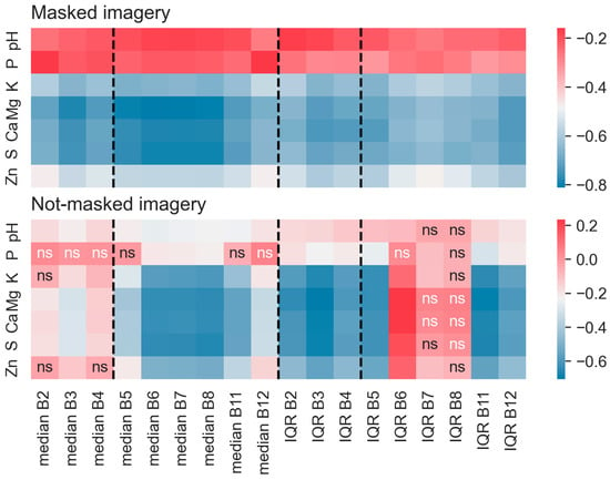
Figure 3.
Correlation analysis between band statistics for pixels spatially coincident with soil fertility measurements. The panel showing masked imagery (top) shows a stronger correlation between measured soil variables and reflectance bands than the panel for not-masked imagery (bottom). The bottom panel likely indicates some confounding influence of vegetation in the relationship. Cells not showing “ns” indicate relationships that are statistically significant at p < 0.05. Dashed lines separate the visible bands from the infrared bands of the spectrum. The study site is in Washington County, Western Mississippi, USA.
The vegetation masking algorithm implemented in GEE from the hand-selected training data was highly accurate (>99% accuracy, Figure 4). The y-axis indicates the number of observations giving the true value of the classification, while the x-axis indicates the number of observations giving the predicted value of the classification. For instance, 1352 observations were correctly predicted to be vegetation, and 1 observation was predicted to be soil when it was in fact vegetation. The remaining 1904 validation observations were correctly classified. No pixels predicted to be vegetation were found to be bare soil pixels. Seasonal changes associated with cropping patterns and changes after planting were evident after applying the vegetation masking model to the images in the Sentinel library within analyzed dates (between June and October, from 2019 to 2023) (Figure 5). The image from July 2021 shows similarities to the image from July 2023 in terms of patterns of where crops have been planted and their stages of growth and greening during the growing season, but some areas that have had bare soil are showing likely vegetation and vice versa. The vegetation masking model captures these trends. Likewise, the large change in greening from June 2023 to late July 2023 captures a quick change in vegetation cover associated with crop growth from the early to the middle parts of the growing season for the crops grown at the site.
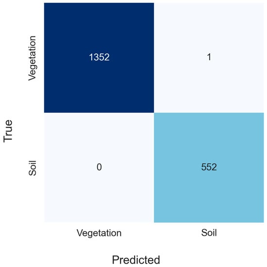
Figure 4.
Validation dataset observations for classes were predicted by the vegetation masking model. The color ramp from white to dark blue indicates the number of responses. The study site is in Washington County, Western Mississippi, USA.
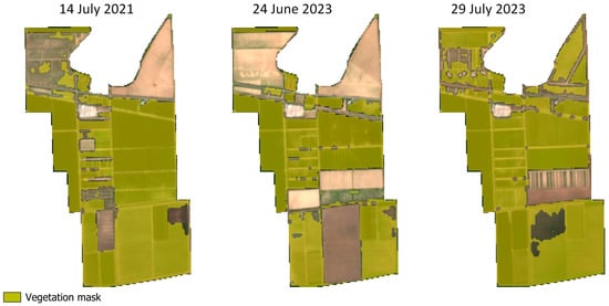
Figure 5.
The vegetation mask developed with random forest classification was applied to all scenes in the S2 library for the research site. Here the vegetation mask is depicted in greenish yellow draped over true color images from Sentinel-2. Individual pixels of each scene in the catalog were tagged as non-data if they were classed as vegetation in the vegetation masking workflow.
The next two figures (Figure 6 and Figure 7) show the influence of sample size on the effectiveness of models built with S2 data that underwent vegetation masking compared to models developed with not-masked S2 data. Overall, as the sample size increased to about 40 samples, model performance improved greatly for K, Mg, Ca, and S. The model improvement was greatest for the masked datasets when using only median bands or when using both median and IQR bands as explanatory variables. Models trained with not-masked median data presented the lowest performance per sample density increase, but their performance noticeably improved after IQR data was added. Still, models that used not-masked data generated less accurate predictions than their masked counterparts.
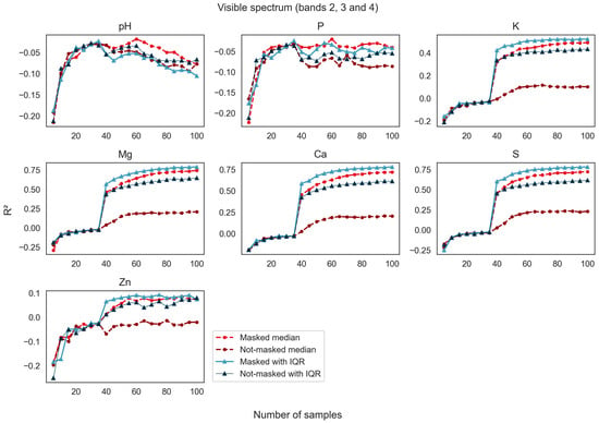
Figure 6.
R2 values report the goodness of fit among spatial estimation models using bands 2, 3, and 4 where pixels were masked and not-masked and whether respective band IQR values were used as an input with an increasing number of soil samples used to train the model.
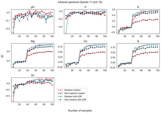
Figure 7.
Models of soil fertility generated using only short-wave infrared portions of the spectrum (bands 11 and 12) increased in performance as the sample size was increased. The images made using median pixel values prior to vegetation masking (not-masked) performed better in this portion of the spectrum than models using the visible spectrum. The R2 values report the goodness of fit between the models made with these limited portions of available soil point data and the data withheld from model development. The study site is in Washington County, Western Mississippi, USA.
Model performance for prediction of soil variables using spectral bands in the visible portion of the spectrum showed R2 values approaching 0.75 for Mg, Ca, and S, the three analytes that were the most predictable as the sample size was increased to 100 samples (Figure 6). Potassium, while being less predictable than Mg, Ca, and S, nevertheless showed a strong increase in model strength when the median reflectance composites were masked. The variables pH, P, and Zn were not adequately predicted by spectral bands in the visible range using this modeling approach. Models built using the median pixel values of the time series of images after masking to remove pixels depicting vegetation (labeled masked median in Figure 6) were superior to their not-masked counterparts in all models. Like models in the visible range of the spectrum, prediction performance using spectral bands in the short-wave infrared portions of the spectrum showed R2 values approaching or higher than 0.75 for Mg, Ca, and S, and values approaching 0.6 for K (Figure 7). Overall, not-masked median bands performed better in shortwave bands than in the visible portion of the spectrum. Here too, the masked S2 reflectance data supported better model performance for nutrient predictions than the not-masked S2 data, but the improvement from masking was more modest.
Models using the entire available soil point data with the S2 reflectance data (1716 point samples for training and 429 for independent validation) performed very well as expected for several soil nutrients but not well for others (Table 3).

Table 3.
Histogram-based gradient boosting model performance for predicting measured soil properties using all the sampled soil point data built from time-series analysis of S2 scenes to predict soil fertility characteristics using (a) S2 scenes after application of a vegetation masking algorithm, and (b) S2 scenes with no vegetation masking algorithm.
Map visualizations of model output for predicted soil nutrients with high prediction efficacy showed strong spatial aggregation for Ca, K, Mg, and S (Figure 8). Models for P, Zn, and pH, however, showed little spatial aggregation and almost no prediction efficacy. This implies satellite reflectance data had very little, if any, ability to elucidate spatial patterns of P, Zn, and pH at the site. For Ca, K, Mg, and S, strong and accurate predictions showed bimodal distributions, with fields at the south of the study site having much higher levels of nutrients. Furthermore, the spatial patterns of these nutrients showed a high degree of aggregation coincident with the boundaries of fields, implying a strong relationship between field nutrient management and reflectance characteristics. Spatial visualizations of band reflectance data after vegetation masking are shown in the Supplemental Materials (Figure S3).
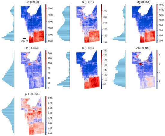
Figure 8.
Spatial models of soil nutrient distribution for surface soils at the research site in Western Mississippi were made using histogram-based gradient boosting applied to measured soil properties and composite images of time-series statistical summaries of multiple images of S2 satellite reflectance values. Histogram values showing the distributions in feature space for the measured soil properties are indicated to the left of each map. The color ramp from blue to red indicates increasing predicted concentrations of the soil property of interest. The R2 value for each prediction surface is given in parentheses above each site map. The study site is in Washington County, Western Mississippi, USA.
The relative importance in the models of the composite median and IQR images calculated from the time series of S2 data indicates that some bands are more useful for distinguishing soil fertility variability than others (Figure 9). The most useful bands for modeling were from the short-wave infrared range, which are also the bands that were least influenced by variability in vegetation characteristics. The models with the best fit were most strongly aided by median composite bands 11 and 8 in their ability to minimize the decrease in R2 in nutrient predictions. Median values of bands 12, 6, and 7 were also among the most important, as was the IQR of band 12.
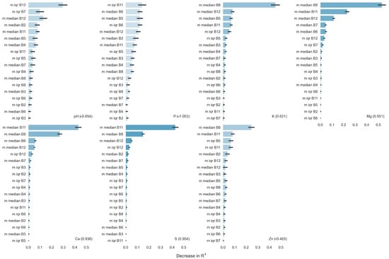
Figure 9.
Variable importance metrics for the IQR and median band composites. To determine the importance of each variable, models were constructed by randomly shuffling the data of the indicated variable, thereby rendering it meaningless, and then tabulating the decrease in the R2 between predicted and measured soil property value. The decrease in R2 associated with excluding the variable is plotted. Model R2 values for each predicted property are given in parentheses at the bottom of each figure. The strength of model R2 is also indicated by the degree of shading of the bars (darker shade of blue is stronger). The term ‘median’ refers to the median composite image in the time series, and ‘IQR’ refers to the interquartile range composite image for each indicated band of S2 satellite reflectance data. The study site is in Washington County, Western Mississippi, USA.
4. Discussion
Satellite imagery is a useful proxy for examining the variability of soil fertility in a floodplain agricultural soil because soil properties that relate to soil fertility variability influence the reflectance characteristics of the soil surface. The variables that were reliably predicted by models at the study site were Ca, Mg, K, and S. These four nutrients are bound within the cation exchange capacity (CEC) of soils and strongly associated with the organic matter complexes in relatively high numbers, and their concentrations often follow the trend of the variability of soil characteristics that dominate CEC, namely SOM and clay content [1]. In A horizons, in most temperate regions, a vast majority of the S in soils is in the organic form, meaning that S content should be strongly correlated with soil organic matter content [1]. Soils at the southern end of the study have greater clay content, greater SOM content, poorer drainage, and darker color. Increases in SOM, clay content, and moisture all decrease a soil’s albedo [14,21], thereby supporting a strong relationship between reflectance intensity as measured by satellite and measured soil properties dominated by CEC. This reliable relationship was useful for modeling soil nutrient spatial variability.
Prior to vegetation masking, the variability of reflectance due to vegetation was higher, as seen in the higher IQR of the reflectance data (Table 2). The IQR from bands 6, 7, and 8 were strongly influenced by the reflectance of infrared light from vegetation. The increased variability of these bands was not meaningfully related to soil fertility and likely reflected variability in vegetation characteristics not pertaining to soil fertility but perhaps to crop choice, variable planting dates, cropping intensity, or other factors (Figure 3). One exception to this observation is the IQR of the not-masked image representing band 5, which is better correlated to soil fertility variables than its masked counterpart. A similar effect was seen in band 11 and band 3.
Interestingly, the advantage conferred by masking vegetation (as seen in Figure 6 and Figure 7) did not translate to the full dataset. In fact, model performance for the models using not-masked S2 data was just as good as, or sometimes better than, models from the vegetation-masked dataset. This is likely because the density of soil samples was so high that nearly any spatial estimation method would likely produce relatively successful models.
The variables that were not as successfully modeled, pH, P, and Zn, have a more complex relationship to reflectance data and do not show reliable correlations at the site. Both pH and P were highly managed variables. P is a macronutrient that can have field-to-field variability relating to applications of P fertilizers related to management goals and cropping requirements. Soil pH is actively managed with lime and can vary greatly depending on management strategies based on crop tolerances.
The number of soil observations taken at this study site was intended to comprehensively characterize the soil nutrient variability. The sampling density was far greater than typical for such agricultural studies and was, in retrospect, excessive to the needs of the study. In a separate study, researchers looking at this dataset estimated that the sampling density required for adequate characterization of the soil variability for this site was on the order of 1 sample per 2.5 hectares, or about 100 samples for the site [5]. By exceeding this sample density by more than an order of magnitude, we were able to fully characterize the soil nutrient variability and determine the advantage conferred by using satellite reflectance data for continuous spatial estimations. Our data show that when developing models using fewer than 100 samples for the site, masking vegetation as non-data confers a distinct improvement in model performance for the respective nutrients investigated. This advantage is diminished as sampling density increases to the full dataset of 1716 samples used for model development and 429 samples used for model validation. At this high density, any confounding effects of including vegetated pixels in the model were outweighed by the greater density of data.
Masking vegetation can improve soil nutrient models built on satellite reflectance data and a limited set of soil observations. Reflectance data from the surface is documented to be different for different soil properties, so reflectance properties provide real information about the soils. Vegetation cover blocks the satellite view of the soil surface and degrades the effectiveness of the ability of the gradient boosting model to predict soil fertility response variables. Masking greatly improved models produced by datasets with point samples intentionally reduced well below the complete dataset. In all bands except Band 3, the IQR of images that did not undergo vegetation masking was greater than for the images with masked vegetation, implying greater consistency and homogeneity in the scenes with vegetation masked as non-data. This gives further evidence that S2 reflectance data provides useful covariate information for predicting soil properties of K, Mg, Ca, and S, especially when masking vegetation.
5. Conclusions
Composite images representing time-series statistics from spectral data from satellites were useful for predicting the spatial variability of soil fertility measurements for K, Mg, Ca, and S at a low-relief floodplain agricultural site. Further investigation is needed to determine if other methods can estimate pH, P, and Zn. The vegetation masking procedure described herein using GEE was a successful approach to isolating bare soil pixels that best-represented reflectance data for soils versus soils and vegetation combined. As such, the method described could be readily replicated and can be applied using S2 or other satellite-based remotely sensed data products at other site locations. The application scope of this method is directed toward floodplain landscapes with soil variability that can be related to reflectance characteristics where vegetation potentially hinders direct observation of soil reflectance. The masking technique allows for automated summary statistics of reflectance values from scenes during unvegetated intervals. Further application and analysis in other landscapes and land uses is warranted. Using time-series pixel-based statistics of satellite reflectance data over time as predictor variables also has a strong utility by providing covariates for predicting nutrient concentrations at the site, particularly soil nutrients associated with the CEC complex. When modeling pixel-based statistics of reflectance variables over time to predict soil nutrients, vegetation interferes with prediction, and masking it could improve nutrient concentration predictions.
Supplementary Materials
The following supporting information can be downloaded at: https://www.mdpi.com/article/10.3390/rs16173297/s1. Figure S1: Histograms showing the total number of soil observations by value bin for the study site for all measured soil nutrients and pH; Figure S2: Dendograms and correlation matrices of S2 band composites from reflectance data at the study site; Figure S3. Intensity of reflectance by S2 band for the research study site; and Table S1: Measured soil property values and geographic locations of observations.
Author Contributions
Conceptualization, P.R.O., M.M., J.M.B. and H.E.W.; methodology, M.M., J.M.B. and H.E.W.; validation, M.M.; formal analysis, M.M.; investigation, M.M., J.M.B., Z.L., P.R.O., A.J.A. and H.E.W.; resources, P.R.O., A.J.A., D.M.M. and S.H.G.S.; data curation, M.M., J.M.B., Z.L., H.E.W., P.R.O. and A.J.A.; writing—original draft preparation, H.E.W. and M.M.; writing—review and editing, M.M., J.M.B., Z.L., P.R.O., A.J.A., H.E.W., D.M.M. and S.H.G.S.; visualization, M.M., Z.L., J.M.B. and H.E.W.; supervision, P.R.O. and A.J.A.; project administration, P.R.O. and A.J.A.; funding acquisition, P.R.O., A.J.A., D.M.M. and S.H.G.S. All authors have read and agreed to the published version of the manuscript.
Funding
Funding was provided by National Institute of Food and Agriculture Award #2022-67013-37319. This research used resources provided by the SCINet project of the USDA Agricultural Research Service, ARS project number 0500-00093-001-00-D.
Data Availability Statement
Soil fertility measurements for point locations are given in tabular format in the attached Supplemental Materials. Remote sensing and elevation data used in this study are publicly available.
Acknowledgments
Authors appreciate CNPq, CAPES, and FAPEMIG for supporting this research, USDA-ARS Sustainable Water Management Research Unit employees James Dean and Roderick Patterson for their crucial assistance in soil sampling, and Poultry Production and Product Safety Unit employee Taylor Adams for sample laboratory analysis.
Conflicts of Interest
The authors declare no conflicts of interest.
References
- Brady, N.C.; Weil, R.R. The Nature and Properties of Soils, 13th ed.; Prentice Hall: Upper Saddle River, NJ, USA, 2002. [Google Scholar]
- Schaetzl, R.J.; Anderson, S. Soils: Genesis and Geomorphology; University Press: Cambridge, UK, 2005. [Google Scholar]
- Iqbal, J.; Read, J.J.; Thomasson, A.J.; Jenkins, J.N. Relationships between Soil-Landscape and Dryland Cotton Lint Yield. Soil Sci. Soc. Am. J. 2005, 69, 872–882. [Google Scholar] [CrossRef]
- Winzeler, H.E.; Owens, P.R.; Joern, B.C.; Camberato, J.J.; Lee, B.D.; Anderson, D.E.; Smith, D.R. Potassium Fertility and Terrain Attributes in a Fragiudalf Drainage Catena. Soil Sci. Soc. Am. J. 2008, 72, 1311–1320. [Google Scholar] [CrossRef]
- Mancini, M.; Winzeler, H.E.; Blackstock, J.; Owens, P.R.; Miller, D.M.; Silva, S.H.G.; Ashworth, A.J. Pixel-Based Spatiotemporal Statistics from Remotely Sensed Imagery Improves Spatial Predictions and Sampling Strategies of Alluvial Soils. Geoderma 2024, 447, 116919. [Google Scholar] [CrossRef]
- Scull, P.; Franklin, J.; Chadwick, O.A.; McArthur, D. Predictive Soil Mapping: A Review. Prog. Phys. Geogr. Earth Environ. 2003, 27, 171–197. [Google Scholar] [CrossRef]
- Mendes, W.D.S.; Demattê, J.A.M.; Silvero, N.E.Q.; Rabelo Campos, L. Integration of Multispectral and Hyperspectral Data to Map Magnetic Susceptibility and Soil Attributes at Depth: A Novel Framework. Geoderma 2021, 385, 114885. [Google Scholar] [CrossRef]
- Guo, L.; Fu, P.; Shi, T.; Chen, Y.; Zeng, C.; Zhang, H.; Wang, S. Exploring Influence Factors in Mapping Soil Organic Carbon on Low-Relief Agricultural Lands Using Time Series of Remote Sensing Data. Soil Tillage Res. 2021, 210, 104982. [Google Scholar] [CrossRef]
- Saucier, R.T.; United States Army Engineer Waterways Experiment Station; United States Mississippi River Commission. Geomorphology and Quaternary Geologic History of the Lower Mississippi Valley; U.S. Army Engineer Waterways Experiment Station: Vicksburg, MS, USA, 1994.
- Vaudour, E.; Gomez, C.; Fouad, Y.; Lagacherie, P. Sentinel-2 Image Capacities to Predict Common Topsoil Properties of Temperate and Mediterranean Agroecosystems. Remote Sens. Environ. 2019, 223, 21–33. [Google Scholar] [CrossRef]
- Vaudour, E.; Gholizadeh, A.; Castaldi, F.; Saberioon, M.; Borůvka, L.; Urbina-Salazar, D.; Fouad, Y.; Arrouays, D.; Richer-de-Forges, A.C.; Biney, J.; et al. Satellite Imagery to Map Topsoil Organic Carbon Content over Cultivated Areas: An Overview. Remote Sens. 2022, 14, 2917. [Google Scholar] [CrossRef]
- Vaudour, E.; Gomez, C.; Lagacherie, P.; Loiseau, T.; Baghdadi, N.; Urbina-Salazar, D.; Loubet, B.; Arrouays, D. Temporal Mosaicking Approaches of Sentinel-2 Images for Extending Topsoil Organic Carbon Content Mapping in Croplands. Int. J. Appl. Earth Obs. Geoinf. 2021, 96, 102277. [Google Scholar] [CrossRef]
- Dvorakova, K.; Heiden, U.; Pepers, K.; Staats, G.; Van Os, G.; Van Wesemael, B. Improving Soil Organic Carbon Predictions from a Sentinel–2 Soil Composite by Assessing Surface Conditions and Uncertainties. Geoderma 2023, 429, 116128. [Google Scholar] [CrossRef]
- Dvorakova, K.; Shi, P.; Limbourg, Q.; van Wesemael, B. Soil Organic Carbon Mapping from Remote Sensing: The Effect of Crop Residues. Remote Sens. 2020, 12, 1913. [Google Scholar] [CrossRef]
- Demattê, J.A.M.; Fongaro, C.T.; Rizzo, R.; Safanelli, J.L. Geospatial Soil Sensing System (GEOS3): A Powerful Data Mining Procedure to Retrieve Soil Spectral Reflectance from Satellite Images. Remote Sens. Environ. 2018, 212, 161–175. [Google Scholar] [CrossRef]
- Guo, L.; Sun, X.; Fu, P.; Shi, T.; Dang, L.; Chen, Y.; Linderman, M.; Zhang, G.; Zhang, Y.; Jiang, Q.; et al. Mapping Soil Organic Carbon Stock by Hyperspectral and Time-Series Multispectral Remote Sensing Images in Low-Relief Agricultural Areas. Geoderma 2021, 398, 115118. [Google Scholar] [CrossRef]
- Fordyce, S.I.; Carr, P.M.; Jones, C.; Eberly, J.O.; Sigler, W.A.; Ewing, S.; Powell, S.L. Sentinel-2-Based Predictions of Soil Depth to Inform Water and Nutrient Retention Strategies in Dryland Wheat. Agric. Water Manag. 2023, 289, 108524. [Google Scholar] [CrossRef]
- Hengl, T.; Miller, M.A.E.; Krizan, J.; Shepherd, K.D.; Sila, A.; Kilibarda, M.; Antonijevic, O.; Glusica, L.; Dobermann, A.; Haefele, S.M.; et al. African Soil Properties and Nutrients Mapped at 30 m Spatial Resolution Using Two-Scale Ensemble Machine Learning. Sci. Rep. 2021, 11, 6130. [Google Scholar] [CrossRef]
- Jobbágy, E.G.; Jackson, R.B. The Distribution of Soil Nutrients with Depth: Global Patterns and the Imprint of Plants. Biogeochemistry 2001, 53, 51–77. [Google Scholar] [CrossRef]
- Van Der Werff, H.; Van Der Meer, F. Sentinel-2 for Mapping Iron Absorption Feature Parameters. Remote Sens. 2015, 7, 12635–12653. [Google Scholar] [CrossRef]
- Bhadra, S.K.; Bhavanarayana, M. Estimation of the Influence of Soil Moisture on Soil Colour. Z. Für Pflanzenernährung Und Bodenkd. 1997, 160, 401–405. [Google Scholar] [CrossRef]
- Xu, X.; Zhai, X. Mapping Soil Organic Matter Content during the Bare Soil Period by Using Satellite Data and an Improved Deep Learning Network. Sustainability 2022, 15, 323. [Google Scholar] [CrossRef]
- Morris, W.M.; Eason, W.P. Soil Survey, Washington County, Mississippi; U.S. Government Printing Office: Washington, DC, USA, 1961.
- Mehlich, A. Mehlich 3 Soil Test Extractant: A Modification of Mehlich 2 Extractant. Commun. Soil Sci. Plant Anal. 1984, 15, 1409–1416. [Google Scholar] [CrossRef]
- Soltanpour, P.N.; Jones, J.M.B., Jr.; Workman, S.M. Optical Emission Spectrometry. In Methods of Soil Analysis; John Wiley & Sons, Ltd.: Hoboken, NJ, USA, 1983; pp. 29–65. ISBN 978-0-89118-977-0. [Google Scholar]
- R Core Team. R: A Language and Environment for Statistical Computing; R Foundation for Statistical Computing: Vienna, Austria, 2021. [Google Scholar]
- Wickham, H.; Averick, M.; Bryan, J.; Chang, W.; McGowan, L.D.; François, R.; Grolemund, G.; Hayes, A.; Henry, L.; Hester, J.; et al. Welcome to the Tidyverse. J. Open Source Softw. 2019, 4, 1686. [Google Scholar] [CrossRef]
- Kuhn, M. Building Predictive Models in R Using the Caret Package. J. Stat. Softw. 2008, 28, 1–26. [Google Scholar] [CrossRef]
- Hijmans, R.J. Terra: Spatial Data Analysis. 2023. Available online: https://CRAN.R-project.org/package=terra (accessed on 14 June 2024).
- Bivand, R.S.; Pebesma, E.; Gomez-Rubio, V. Applied Spatial Data Analysis with R, 2nd ed.; Springer: New York, NY, USA, 2013. [Google Scholar]
- Pebesma, E.J.; Bivand, R. Classes and Methods for Spatial Data in R. R News 2005, 5, 9–13. [Google Scholar]
- Pebesma, E. Simple Features for R: Standardized Support for Spatial Vector Data. R J. 2018, 10, 439–446. [Google Scholar] [CrossRef]
- Roudier, P. Clhs: A R Package for Conditioned Latin Hypercube Sampling. 2011. Available online: https://cran.r-project.org/web/packages/clhs/index.html (accessed on 14 June 2024).
- Kremer, L.P.M. Ggpointdensity: A Cross between a 2D Density Plot and a Scatter Plot; R Core Team: Vienna, Austria, 2019. [Google Scholar]
- Ranghetti, L.; Boschetti, M.; Nutini, F.; Busetto, L. “Sen2r”: An R Toolbox for Automatically Downloading and Preprocessing Sentinel-2 Satellite Data. Comput. Geosci. 2020, 139, 104473. [Google Scholar] [CrossRef]
- Gorelick, N.; Hancher, M.; Dixon, M.; Ilyushchenko, S.; Thau, D.; Moore, R. Google Earth Engine: Planetary-Scale Geospatial Analysis for Everyone. Remote Sens. Environ. 2017, 202, 18–27. [Google Scholar] [CrossRef]
- U.S. Geological Survey. 20221121, USGS 1 Meter 15 x69y371 MS_Central_Delta_2018_D18. 2022. Available online: https://www.sciencebase.gov/catalog/item/6392d084d34e0de3a1efd555 (accessed on 14 June 2024).
- Quantum Spatial MS_MississippiDelta_2018_D18 Lidar Processing Report. 2020. Available online: https://maris.mississippi.edu/MARISdata/Elevation/LIDAR/MS_Delta_2019to20/UTM_15/metadata/reports/Final_MS_Delta_ProcessingReport_UTM15.pdf (accessed on 14 June 2024).
- U.S. Geological Survey. 3D Elevation Program 1-Meter Resolution Digital Elevation Model (Published 20200606); 2002. Available online: https://www.usgs.gov/3d-elevation-program (accessed on 14 June 2024).
- European Space Agency. Sentinel-2 Mission Guide2024. Available online: https://sentinels.copernicus.eu/web/sentinel/missions/sentinel-2 (accessed on 14 June 2024).
- Ke, G.; Meng, Q.; Finley, T.; Wang, T.; Chen, W.; Ma, W.; Ye, Q.; Liu, T.-Y. LightGBM: A Highly Efficient Gradient Boosting Decision Tree. In Advances in Neural Information Processing Systems; Guyon, I., Von Luxburg, U., Bengio, S., Wallach, H., Fergus, R., Vishwanathan, S., Garnett, R., Eds.; Curran Associates, Inc.: Red Hook, NY, USA, 2017; Volume 30, Available online: https://proceedings.neurips.cc/paper_files/paper/2017/file/6449f44a102fde848669bdd9eb6b76fa-Paper.pdf (accessed on 14 June 2024).
- Diek, S.; Fornallaz, F.; Schaepman, M.E.; De Jong, R. Barest Pixel Composite for Agricultural Areas Using Landsat Time Series. Remote Sens. 2017, 9, 1245. [Google Scholar] [CrossRef]
- Friedman, J.H. Greedy Function Approximation: A Gradient Boosting Machine. Ann. Stat. 2001, 29, 1189–1232. [Google Scholar] [CrossRef]
Disclaimer/Publisher’s Note: The statements, opinions and data contained in all publications are solely those of the individual author(s) and contributor(s) and not of MDPI and/or the editor(s). MDPI and/or the editor(s) disclaim responsibility for any injury to people or property resulting from any ideas, methods, instructions or products referred to in the content. |
© 2024 by the authors. Licensee MDPI, Basel, Switzerland. This article is an open access article distributed under the terms and conditions of the Creative Commons Attribution (CC BY) license (https://creativecommons.org/licenses/by/4.0/).