Article

Sugarcane Mosaic Virus Detection in Maize Using UAS Multispectral Imagery

1
Department of Food, Agricultural, and Biological Engineering, The Ohio State University, Columbus, OH 43201, USA
2
Corn, Soybean and Wheat Quality Research Unit, USDA-ARS, 1680 Madison Ave., Wooster, OH 44691, USA
*
Author to whom correspondence should be addressed.
Remote Sens. 2024, 16(17), 3296; https://doi.org/10.3390/rs16173296
Submission received: 21 May 2024 / Revised: 26 August 2024 / Accepted: 29 August 2024 / Published: 5 September 2024
(This article belongs to the Special Issue Crops and Vegetation Monitoring with Remote/Proximal Sensing II)

Abstract

:
One of the most important and widespread corn/maize virus diseases is maize dwarf mosaic (MDM), which can be induced by sugarcane mosaic virus (SCMV). This study explores a machine learning analysis of five-band multispectral imagery collected via an unmanned aerial system (UAS) during the 2021 and 2022 seasons for SCMV disease detection in corn fields. The three primary objectives are to (i) determine the spectral bands and vegetation indices that are most important or correlated with SCMV infection in corn, (ii) compare spectral signatures of mock-inoculated and SCMV-inoculated plants, and (iii) compare the performance of four machine learning algorithms, including ridge regression, support vector machine (SVM), random forest, and XGBoost, in predicting SCMV during early and late stages in corn. On average, SCMV-inoculated plants had higher reflectance values for blue, green, red, and red-edge bands and lower reflectance for near-infrared as compared to mock-inoculated samples. Across both years, the XGBoost regression model performed best for predicting disease incidence percentage (R2 = 0.29, RMSE = 29.26), and SVM classification performed best for the binary prediction of SCMV-inoculated vs. mock-inoculated samples (72.9% accuracy). Generally, model performances appeared to increase as the season progressed into August and September. According to Shapley additive explanations (SHAP analysis) of the top performing models, the simplified canopy chlorophyll content index (SCCCI) and saturation index (SI) were the vegetation indices that consistently had the strongest impacts on model behavior for SCMV disease regression and classification prediction. The findings of this study demonstrate the potential for the development of UAS image-based tools for farmers, aiming to facilitate the precise identification and mapping of SCMV infection in corn.

Graphical Abstract

1. Introduction

Corn/maize (Zea mays) is one of the most important food crops globally and is the leading staple cereal in terms of annual production, exceeding 1 billion metric tons [1,2]. Ensuring the healthy and sustainable production of corn is, therefore, critical to maintaining food security and successful agricultural development on a global and local scale. One of the greatest challenges for farmers in maintaining profitable corn yields is the sustainable management of pests and pathogens. Annual global yield loss for corn due to pests and pathogens is approximately 22.5% of total yields [3]. One of the most important and widespread virus diseases in corn is maize dwarf mosaic (MDM), which is widely distributed in the USA and abroad.
MDM is induced by viruses in the family Potyviridae, most commonly by maize dwarf mosaic virus (MDMV) or by sugarcane mosaic virus (SCMV) [4]. SCMV infects various grain crops such as corn, sorghum, sugarcane, and other poaceous species, causing severe grain and forage yield losses among susceptible cultivars [4,5]. Monitoring the spread and emergence of new virus variants is critical for disease management [6,7]. Recently, a novel and highly virulent SCMV isolate was discovered in South Asia [8,9]. Furthermore, potyviruses are known to enhance other virus diseases. Notably, maize lethal necrosis (MLN) disease, caused by co-infection with maize chlorotic mottle virus and a potyvirus, devastated corn production in regions of East Africa, Southeast Asia, and South America [10,11,12,13]. The widespread distribution and diversity of MDM-inducing potyviruses, combined with their ability to cause severe disease individually or in co-infection with other viruses, highlight the long-term threat SCMV poses for the cultivation of corn and other grains [14,15].
Symptoms associated with MDM include mosaic, chlorosis, plant stunting, reduced biomass, and small ear size [16,17]. Early symptoms in young leaves appear as irregular, light, or dark green mosaicking or mottling patterns that may develop into greenish or yellowish streaks along the veins of the corn leaves [14]. Overall, visual symptoms alone are often insufficient for a positive identification of SCMV infection, and, thus, serological or molecular diagnostic tests are needed [14]. Currently, the preferred method for controlling SCMV is to grow resistant corn varieties. However, most commercial field corn hybrids commercially available in the USA are only partially resistant to SCMV and many sweet corn lines and varieties are highly susceptible to both MDMV and SCMV [18,19,20,21]. Furthermore, changes in climate, seasonal patterns, and extreme weather events may shift spatial and temporal SCMV population dynamics as well as the levels of SCMV virulence. For these reasons, the proactive development of better monitoring and identification techniques for virus detection is critical.
The early identification and continuous monitoring of pests and pathogens are key components in effective disease management and can help improve yields while also minimizing environmentally and economically costly control methods. Remote sensing leverages electromagnetic radiation as the information carrier [22], and so by capturing crop health information in the form of spectral signatures that cannot be detected by the human eye during traditional scouting approaches, multispectral remote sensing may provide an efficient and scalable approach to monitoring pathogen impacts [23]. UAS technology plays a vital role in precision agriculture by supporting the four pillars of farm input management: applying the right practice, at the right place, at the right time, and in the right quantity [24]. From pre-season planning to post-harvest, UAS technology can be integrated into every stage of production agriculture, enabling the collection of high-spatial- and -temporal-resolution images that can support efficient decision making, reductions in costs, and potential increases in yield and profit [24]. Since 2015, the use of UAS-based remote sensing has seen a sharp increase in agricultural applications [25], and there are now techniques that use spectral signatures, collected in the visible to near-infrared wavelengths by a multispectral sensor, to assess vegetation health. Specifically, vegetation indices derived from a combination of various spectral bands are useful in assessing the structural, physiological, or biochemical properties of vegetation [26,27,28,29]. Typically, healthy vegetation reflects large portions of near-infrared light and absorbs blue and red light for photosynthetic processes and chlorophyll production [30]. The reflectance spectra of vegetation can be analyzed via machine learning methods to identify anomalies or unique vegetation characteristics such as the presence of disease or nutrient stresses [25,31,32].
Several studies have investigated the spectral characteristics of mosaic viruses in crops, such as mosaic virus in sugarcane [33,34], mungbean yellow mosaic India virus in soybeans [35], wheat streak mosaic virus in wheat [36], and yellow mosaic disease in black beans [37]. In 2018, Moriya et al. [31] mapped the mosaic virus in sugarcane using in-field identification, spectroradiometer readings, and UAS-collected hyperspectral imagery. This involved creating a spectral reference library for healthy and infected leaves, weeds, and bare soil, followed by a spectral information divergence classification process of collected hyperspectral orthomosaics. The study successfully classified 74 out of 80 samples. Another similar study [34] used satellite imagery and the random forest algorithm to classify maize streak virus in corn, showing that the inclusion of vegetation indices as compared to images only improved classification accuracy by 3.4%, reaching 82.75%. However, hyperspectral imagery is expensive and complex to process, and satellite imagery has spatial resolution limitations.
Specific to corn, there have been a handful of studies that have investigated the spectral signatures of diseases, including foliar fungal diseases [29], maize dwarf mosaic virus [38,39], maize streak virus [40,41,42], northern leaf blight [43,44,45], grey leaf spot [46], and tar spot complex [47]. These studies utilize various spectral methodologies and data types, including multispectral satellite data, UAS-collected RGB/multispectral images, and proximal spectroradiometer reflectance measurements. However, to our knowledge, there have been no prior studies investigating the unique spectral characteristics of SCMV in corn and its corresponding relation to yields.
This study integrates a machine learning analysis of multispectral imagery collected via UAS for disease detection, focusing on three objectives: (i) identifying the most important/correlated spectral bands and vegetation indices with SCMV infection, (ii) comparing spectral signatures of mock-inoculated (noninfected) and SCMV-inoculated (infected) corn plants, and (iii) evaluating model prediction performances for four algorithms concerning early and late infections of SCMV.

2. Materials and Methods

2.1. Study Area and Experimental Setup

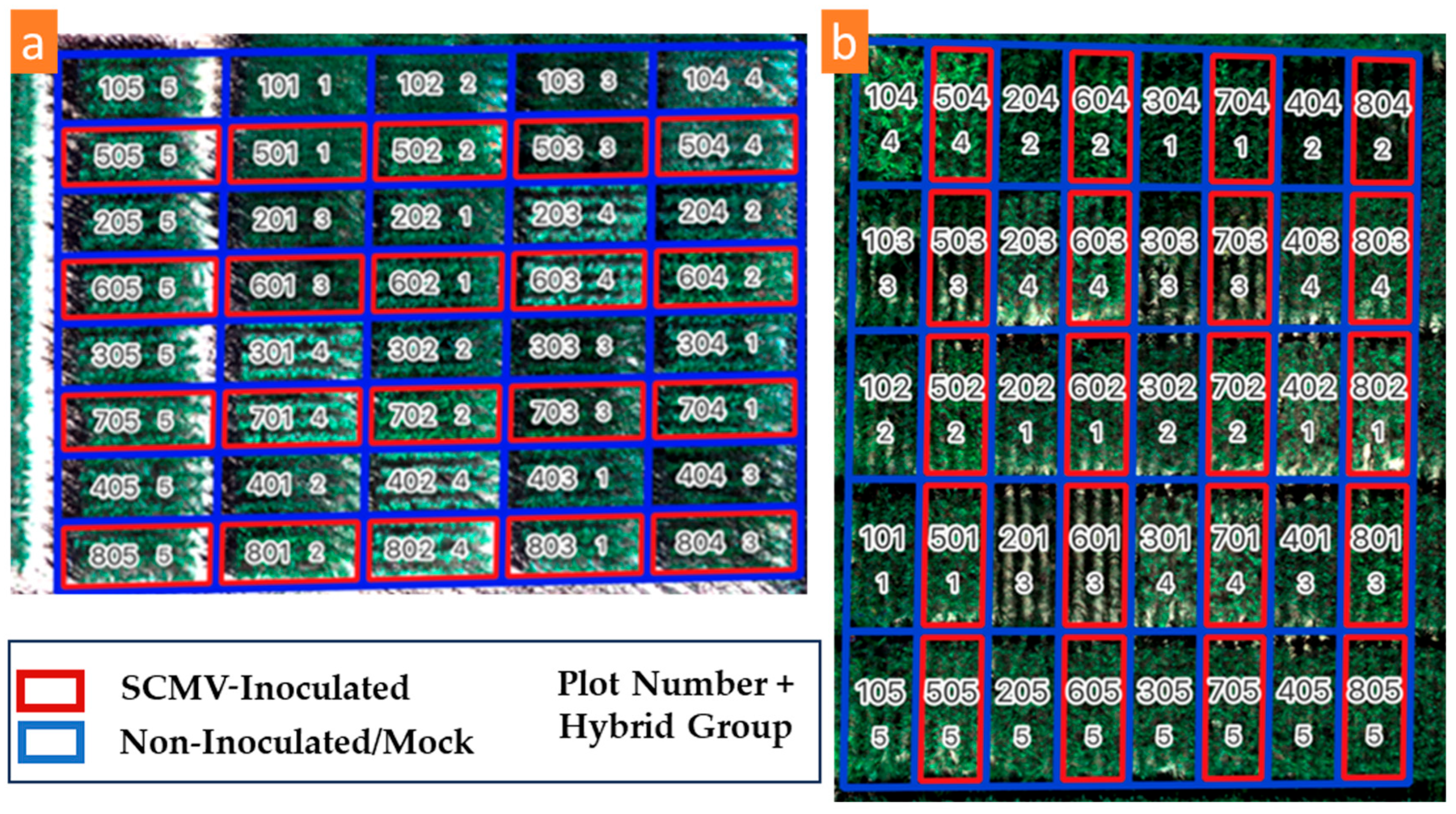
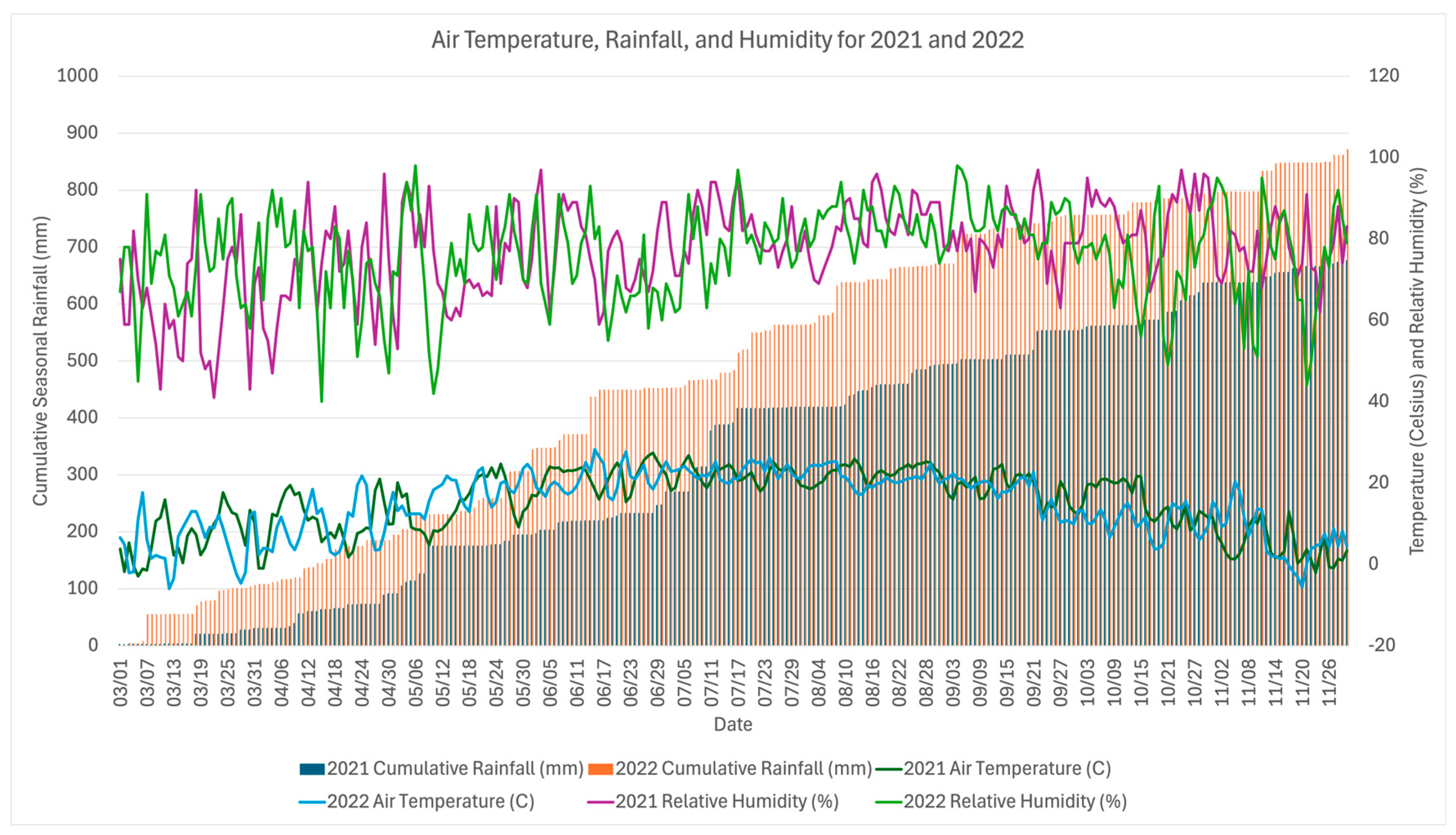
Experiments were conducted during corn growing seasons in 2021 and 2022 on research plots at Snyder and Schaffter Farms of the Ohio State University (OSU) located in Wooster, OH, USA (Figure 1 and Figure 2). The Snyder Farm plots were approximately 0.64 acres in 2021 and 0.33 acres in 2022, containing Canfield silt loam soils. The 2022 Schaffter Farm plots were approximately 0.37 acres in size, containing Wooster-Riddles silt loams. Air temperature and relative humidity were similar for both years; however, the cumulative rainfall was greater for 2022 than for 2021 (Figure 3).
Forty-eight commercial field corn hybrid varieties, provided by Rich Minyo, OSU, from the remnant seed of the Ohio Corn Performance Tests, were evaluated using a randomized block design in the 2021 field experiment. These varieties represent some of the highest-yielding varieties currently available from five major commercial seed companies and were found to be susceptible to SCMV from previous trials [20]. Thus, three in-house hybrid controls were used as SCMV-resistant (Oh28 × Pa405; Oh28 × Oh1VI) and -susceptible (Wf9 × Oh51A) controls. Seeds were planted with a Kinze 2100 planter (Kinze Manufacturing, Williamsburg, IA, USA) with Almaco seed distribution cones in single-row plots on May 20 in 2021.
Based on the 2021 field experiment, four susceptible varieties were selected from the 48 commercial hybrids for more in-depth characterization in the 2022 experiment, considering their disease incidence scores and yield penalty due to infection. Three hybrid controls were used in 2021 and Wf9 × Oh51A (hybrid 4)-susceptible control was used in 2022 to evaluate disease pressure and uniformity of inoculation. Seeds were planted in four-row plots on 23 May 2022. In each year, there were four replications per hybrid for each treatment (Figure 1 and Figure 2). Row length was 6.7 m with 35 kernels per row. Rows were 0.76 m in width. For both years, the best agronomic practices achieved optimal yields without irrigation, as well as without the application of insecticides or fungicides.
The replicates included both SCMV-inoculated and mock-inoculated treatments (Figure 1). In 2021, Snyder Field had a total of 408 hybrid sample plots (rows) (51 hybrids with 4 replicates each). In 2022, each field had a total of 40 hybrid sample plots (blocks). Hybrids were inoculated as previously described in [19]. Briefly, SCMV-infected plant tissues were homogenized using a commercial blender in 0.01 M potassium phosphate buffer in a 1:10 wt/v ratio. The homogenate was filtered through fine cheesecloth. Then, 2 g of carborundum was mixed with 6 L of inoculum and applied using a gas-powered mist blower (Model 452 Solo, Newport News, VA, USA) at an approximate application rate of 1 L per 75 m. Mock inoculations were similarly applied using only 0.01 M potassium phosphate buffer and carborundum. Plants were inoculated between the V3 and V5 maturity stages. Inoculations were performed five times at five-day intervals between June and July (18 June, 24 June, 29 June, 1 July, and 6 July) in 2021 and four times (17 June, 22 June, 27 June, and 1 July) in 2022.

2.2. Data Collection

2.2.1. Imagery via UAS Flights

UAS flights were conducted using a DJI Matrice 200 drone (DJI, Shenzhen, China) on three dates each year for each field—(28 June, 14 July, and 28 July) in 2021 and (30 June, 28 June, and 1 September) in 2022—to capture trends in the spectral signatures of corn plants resulting from inoculations. During these flights, multispectral imagery with five spectral bands was collected using a MicaSense RedEdge-MX multispectral sensor (MicaSense, Seattle, WA, USA) at an altitude of 30m. The flights maintained a 75% front-overlap and 75% side-overlap, following a lawnmower pattern. To ensure the spatial accuracy of images respective to treatments on the field, four permanent ground control points (GCPs) were positioned at the corners of each corn field and remained visible and undisturbed throughout the growing season. Precise GPS coordinates for these GCPs were recorded using a Trimble real-time kinetic (RTK) GPS system (Trimble, Westminster, CO, USA).
Additional thermal imagery was collected with a DJI Zenmuse XT2 sensor (DJI, Shenzhen, China) using the same drone at an altitude of 20m with a 90% front-overlap and 90% side-overlap. Due to challenges in stitching the orthomosaic thermal images, usable images were obtained only for 28 June 2021 (Snyder), 14 July 2021 (Snyder), 30 June 2022 (Snyder), 30 June 2022 (Schaffter), 28 July 2022 (Snyder), and 1 September 2022 (Snyder).
LiDAR data were also collected using a Free Fly Alta X drone (Freefly Systems, Woodinville, WA, USA) at an altitude of 44m using a Velodyne VLP-16 Hi-Res sensor (Velodyne, San Jose, CA, USA). LiDAR data were collected for both fields only on 28 July 2022 to assess differences in canopy heights between treatments. For additional details on the data used in model development, refer to the subscript description in Table 1.

2.2.2. Grain Yield

Yield values were recorded at the end of the season during harvest on 9 November 2021 and 21 November 2022 using a tractor-mounted yield monitor. Weight, moisture percentage, and bushels were used to calculate the standard ‘bushels per acre’ metric for each hybrid plot/block, and these values were interpreted as ‘ground truth’ yield values. Yields were normalized to a standard 15.5% moisture content and reported as kg/ha (or Bu/A).

2.2.3. Plant Disease Incidence

The percentage of plants that displayed mosaic symptoms for each hybrid plot was recorded using human scouting. Plant disease was evaluated based on the presence or absence of visible mosaic symptoms. Disease incidence for each hybrid variety was calculated based on the number of symptomatic plants divided by the final stand count. During 2021, symptoms were evaluated on 30 June 2021, 8 July 2021, and 12 July 2021. In 2022, the disease incidence scores were recorded on 15 July 2022 and 19 July 2022 for Schaffter Field and on 6 July 2022, 15 July 2022, and 18 July 2022 for Snyder Field. The percentage of plants symptomatic for SCMV within each hybrid sample plot (Figure 1 and Figure 2) was recorded for each date. The value on the final scouting date was interpreted as the respective disease incidence rate and was used in subsequent analyses and modeling.

2.3. Data Processing

2.3.1. UAS Collected Imagery and Plant Reflectance

A flow diagram displaying the general methodological process implemented can be seen in Figure 4. The multispectral images collected by UAS were stitched into single-orthomosaic files of each field for each flight and for each of the five bands using Pix4D Mapper software Version 4.2.27 (Pix4D SA, Lausanne, Switzerland) [48]. To ensure that all images were aligned, the five-band composite files for each flight date were georeferenced based on the GCPs using ArcGIS Pro 3.2.0 software [49]. This process was also performed for the thermal images; however, some dates had stitching issues (see Table 1).
Using the multispectral orthomosaics, mean pixel reflectance values were calculated and extracted for each of the five bands within each individual hybrid sample plot using the zonal statistics function in R v2022.07.0 Build 548 [50] for each field and flight date. To remove spectral noise from soil pixels, only pixels with corn vegetation were considered when summarizing reflectance values. For this, a threshold based on an excess green index, which amplifies green reflectance over red and blue [51,52], was used. In the threshold file, all vegetation pixels are assigned a value of one, and non-vegetation pixels are given a value of zero. For each flight, pixel-wise reflectance data for the five multispectral bands were extracted in R by multiplying each band file by the threshold file to remove non-vegetation pixels and then using an extract function to isolate reflectance values within each hybrid sample plot boundary. The same extraction process was applied to thermal orthomosaic pixels. A crop canopy height model was created from the LiDAR data collected using a .las file in CloudCompare v2.12.3 software [53], with more details reported in the Supplementary Materials.

2.3.2. Vegetation Indices

To further understand the effect of SCMV on corn vigor, 36 vegetation indices based on various combinations of spectral bands were calculated for each plot, alongside the individual spectral bands from multispectral (5) and thermal (1) sensors (Table 2). These vegetation indices include the following: BI, CI, CIG, CIRE, CVI, EVI, GARVI, GNDVI, gWDRVI 1, gWDRVI 2, HI, IRVI, lnRE, MCARI 1, MCARI 2, MCARIOSAVI, MSAVI, MSR, MTVI 1, MTVI 2, NDRE, NDVI, NGRDI, NIR/Green, NIR/Red, NIR/Red-Edge, OSAVI, RDVI, RI, SAVI, SCCCI, SI, TCARI, TCARIOSAVI, WDRVI 1, and WDRVI 2 (see Table 2).

2.4. Statistical Analysis and Machine Learning Models

2.4.1. Model Formation and Performance

A correlation scatterplot matrix was created using the psych library [77] in R [50] to investigate the linear correlation between each pair of available variables/features, including yield, canopy height, thermal value, disease incidence, the five spectral bands, and the 36 vegetation indices for each flight date. Specifically, a Pearson correlation (r) was analyzed for the SCMV-inoculated plots to explore the relationships between the spectral bands/vegetation indices and the ‘disease incidence’ scores. Correlation matrices were generated for all included variables and revealed the presence of multicollinearity, and this informed appropriate model selection. Kruskal–Wallis one-way analysis of variance [78] was also performed to test for statistically significant differences between SCMV-inoculated and mock-inoculated treatments for each of the spectral bands/vegetation indices.
To predict disease incidence and classify disease presence using multispectrally derived features, the performance of four commonly used machine learning models—ridge regression [79], support vector machine (SVM) [80], random forest (RF) [81], and XGBoost [82]—were evaluated. These models have robust capabilities for handling multicollinearity [79,83,84], which is often present among VIs derived using multispectral images. While XGBoost, SVM, and RF were used to predict the presence or absence of SCMV infection, XGBoost, SVM, RF, and ridge regression were used for predicting disease incidences.
For a detailed technical understanding of these algorithms, please see the original articles as cited. The modeling approach taken can be described primarily as a supervised machine learning-based strategy rather than a deep learning- or statistics-based approach [22]. Briefly outlining the selected models, ridge regression is a commonly used multiple regression technique for analyzing data that suffer from multicollinearity [79,85,86]. Ridge regression shrinks model coefficients and can help reduce overfitting and model complexity. The value for the penalty term or regularization parameter, lambda, was optimized for each ridge regression model using a grid search method. Support vector machine regression (SVM or SVR) tends to have very good generalization capability, is robust to outliers, and is effective even when the number of features/predictors is greater than the number of samples/observations [87,88,89]. For both ridge and SVR algorithms, all feature values were scaled to ensure features were contributing equally to the model. Random forest (RF) is a commonly used machine learning algorithm that averages the output of multiple individual regression trees to reach a single result [81]. RF models are an extension of bagging, which also randomly selects subsets of features [90]. RF models tend to be easily interpretable and efficient to train and display high generalization capabilities. XGBoost is a decision tree algorithm that implements regularized gradient boosting [82]. XGBoost training proceeds iteratively as new trees predict residuals of prior trees and then together yield a final result [82]. XGBoost is one of the leading machine learning algorithms, works well with non-scaled data, and is efficient and scalable. The SVM, rF, and XGboost algorithms were implemented in Python with scikit-learn libraries [91], while ridge regression was implemented in R using the caret and glmnet packages.

2.4.2. Model Performance Optimization (Using Multispectrally Derived Data)

The hyperparameters of all SVM, RF, and XGBoost models were optimized using Hyperopt in Python 3.7.16. Hyperopt is a library that provides sequential model-based optimization (also known as Bayesian optimization) for efficient function minimization, such as root mean squared error (RMSE), by exploring differing hyperparameter values [92]. While grid search (used for ridge regression) exhaustively examines all hyperparameter permutations, it becomes computationally demanding for algorithms with many parameters. Hyperopt navigates the hyperparameter space iteratively, leveraging prior evaluations for efficient exploration. Detailed hyperparameter spaces explored for each model are available in the Supplementary Materials (Table S1).
Initial models for predicting disease incidence used only multispectral-derived features, encompassing 5 bands and 36 indices, totaling 41. Models were trained for each individual year and combined years (all available data). Combined models included 888 samples across both years with 768 observations occurring in 2021 and 120 observations occurring in 2022. For this, five-fold cross-validation with a randomized split of 70% and 30% for training and testing sets, respectively, was used. Additionally, we also implemented the assigning of 2021 data for training and 2022 data for the testing of models, specifically for the XGBoost regression and SVM classification models due to their strong performances. Model performances were compared using RMSE and the coefficient of determination (R2) as metrics.
For a more effective analysis of spectral bands and vegetation indices crucial for SCMV infection, a binary classification approach based on inoculation status was considered, rather than relying on a continuous ‘disease incidence’ score prone to human error and environmental factors. Classification models were built with two categories: SCMV-inoculated versus mock-inoculated. For the annotation of the classification models, the inoculated plots, regardless of disease incidence score, were set to values of 1, and non-inoculated plots were set to values of 0. Similar to regression models, all 41 features were incorporated into these classification models.
After identifying the best-performing models with multispectral-derived features, they were simplified using recursive feature elimination (RFE) as a feature selection tool to mitigate overfitting and enhance generalizability. RFE was applied to both years of data with the XGBoost model, maintaining optimized hyperparameters, and this was carried out using boostrfe and shap-hypetune in Python [93]. Following this simplification, feature importance and model behavior were analyzed using SHAP analysis. For the SVM classification model, a confusion matrix [94] was created to summarize SCMV infection status classification performance. Three metrics, including accuracy, precision, and recall, were estimated using predicted and actual observations (Equations (1)–(3)).
In the confusion matrix, true positive (TP) and true negative (TN) are represented by numbers in the diagonal and indicate the model’s ability to accurately detect mock and SCMV inoculations, respectively. False positive (FP) refers to instances where the model predicts mock inoculations as SCMV inoculations. False negative (FN) indicates the model’s failure to detect mock inoculations.
Accuracy   =   T P + T N / T P + F P + T N + F N
Precision   =   T P / T P + F P
Recall   =   T P / T P + F N

2.4.3. Modeling with Additional Available Data

Further models were investigated by incorporating additional features, such as LiDAR-derived canopy height and thermal imagery-based temperature values, to assess potential performance enhancement with data from extra sensors. These models utilized all available data from all sensors, extending beyond multispectral-derived information. XGBoost was selected for training these models due to its consistently superior performance with multispectral-only data. Hyperopt was employed once again to optimize the hyperparameters of these models. Additional variables such as thermal and canopy height that were available across both fields and years (Table 1) were incorporated into these models. This resulted in two additional features, totaling 43 features in the model. This modeling was only performed for all data in aggregate as the additional data occurred sporadically (i.e., both years were used and June dates were included so that all thermal data could be leveraged). Five-fold cross-validation was used with a total of 1059 observations and with a randomized split of 70% and 30% for training and testing sets, respectively.

2.4.4. Shapely Additive Explanations Analysis

SHAP analysis [95] was used to investigate model behavior and examine the influence of each feature on predicting the model output. This analysis was conducted for two best-performing models, one for disease incidence percentage and another for disease classification (inoculation vs. mock). TreeExplainer and KernelExplainer in Python were used for the SHAP analysis, which aids in interpreting the inner workings of machine learning models [96]. Feature importance and impact on model behavior were investigated using bar and summary plots. SHAP values quantify the contribution of each feature to model predictions. While SHAP values do not imply causation, they elucidate how the model behaves concerning predictions. In a SHAP plot, leftward dots along the x-axis indicate negative impacts, while rightward dots indicate a positive influence on the target variable (e.g., disease incidence percentage). The color gradient from red (high feature value) to blue (low value) illustrates feature significance. For instance, a red dot on the left side implies a negative contribution due to a high feature value. Features are ranked by average SHAP value, mirrored in the bar plots showing mean SHAP values along the x-axis, and offering insights into feature importance.

3. Results

3.1. Disease Incidence and Corn Yield

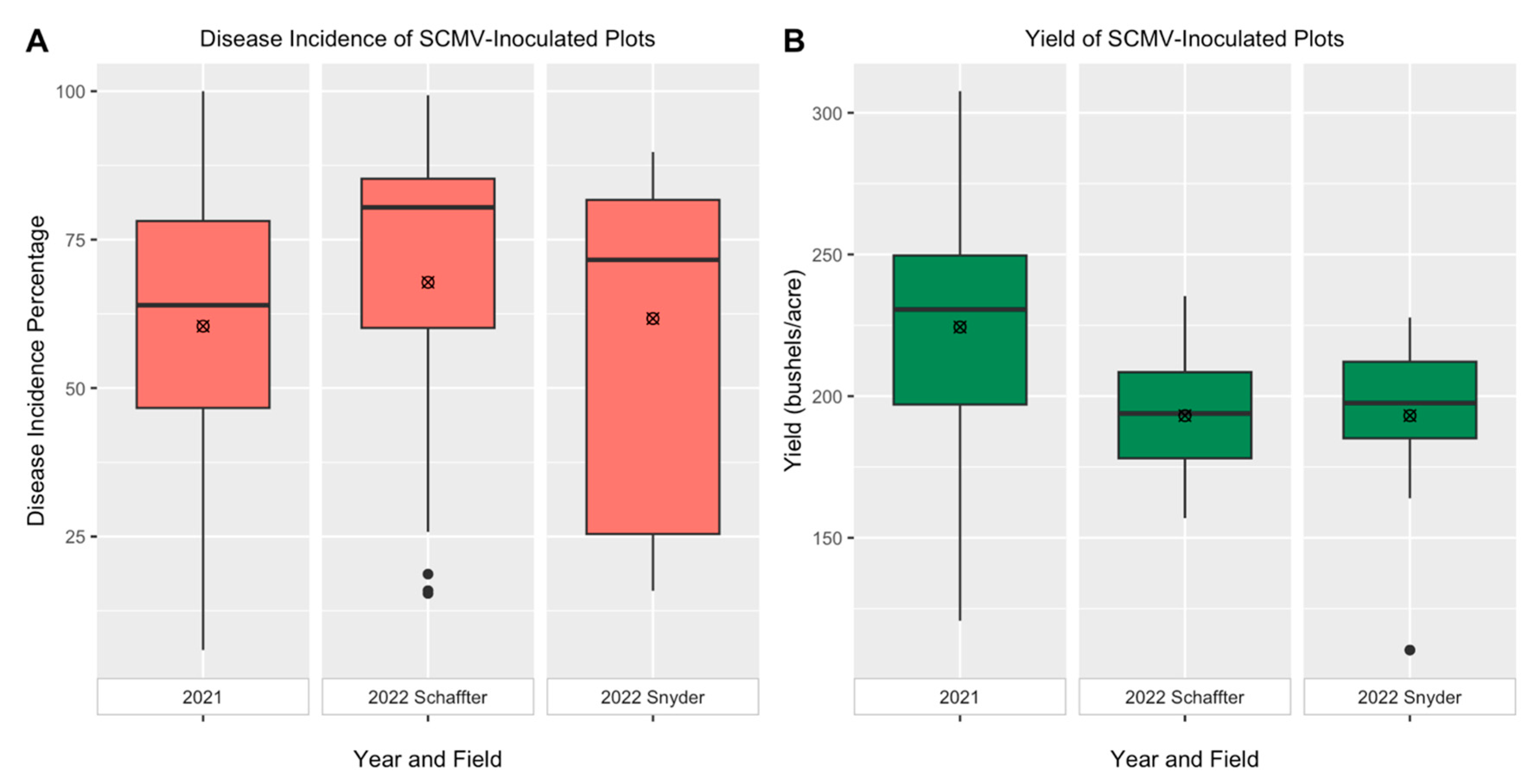
In 2021, disease incidence scores for commercial hybrids at Snyder Farm ranged from 5% to 100%, with median scores of 63% and mean scores of 60% (Figure 5). Susceptible (Wf9 × Oh51A) control had a mean of 96%, resistant (Oh28 × Pa405) control had 6%, and resistant (Oh28 × Oh1VI) control had 0%. Inoculated plot yields averaged 15,090 kg/ha (224 Bu/A), while non-inoculated plots averaged 16,821 kg/ha (250 Bu/A).
In 2022, disease incidence at Synder varied between 15% and 89%, with median and mean scores of 71% and 61%. Hybrid mean disease severities were 70%, 82%, 83%, 76%, and 21% for hybrids 1, 2, 3, 4, and 5, respectively. Mean yields for the inoculated plots were 12,987 kg/ha (193 Bu/A), while non-inoculated plots were 13,123 kg/ha (195 Bu/A).
At Schaffter Farm, disease incidences varied between 15% and 99%, with median and mean scores of 80% and 67%. Hybrid mean disease severities were 78%, 93%, 79%, 80%, and 18%, for hybrids 1, 2, 3, 4, and 5, respectively. The inoculated mean yield was 12,987 kg/ha (193 Bu/A), and the non-inoculated mean was 14,341 kg/ha (213 Bu/A).

3.2. Feature Correlation

Significant relationships between disease incidence and various vegetation indices (or spectral bands) were identified on 14 July 2021. SCCCI, TCARI/OSAVI, MACARI/OSAVI, and CVI showed the most significant correlations, with r values of −0.40, 0.30, 0.30, and 0.26, respectively. On 28 July 2021, SCCCI was found again as the most strongly correlated vegetation index with disease incidence, with an r value of −0.31, followed by NDRE, CIRE, and NIR/Red with r values of −0.24 each.
On 28 July 2022, no significant correlations were detected for disease incidence at Snyder. However, at Schaffter, disease incidence was significantly correlated with the NIR spectral band (r = −0.63), MCARI1 (r = −0.61), and MTVI1 (r = −0.60). On 1 September 2022, towards the later growth stage of corn, significant correlations were discovered at both locations. At Snyder, disease indices were most strongly correlated with NIR, MCARI1, and MTVI1 with r values of −0.63, −0.61, and −0.56, respectively. In Schaffter Field, MCARI2, NIR/Red, and MSR all had the highest r value of 0.56 (Table 3 and Supplementary Table S2). Compared to other VIs or spectral bands, SCCCI and MACRI were identified as consistently capturing variability in disease incidence at a higher percentage.

3.3. Analysis of Variance

On average for both years, SCMV-inoculated plots had a higher reflectance in the visible (red, green, blue) and red-edge portions of the electromagnetic spectrum and a lower average reflectance in the NIR portion as compared to mock-inoculated plots. On 14 July 2021, all bands showed significant differences, with significance in descending order: red, green, near-infrared, red-edge, and blue. On 28 July 2021, only red-edge and green had significant differences. Notably, no statistically significant differences were found in individual flight dates during 2022. Aggregated data for 2021 revealed significant differences in red-edge, red, and near-infrared bands, while no significant differences were found in the 2022 aggregated data (Figure 5, Figure 6, and Figure S1). Please see Figure S1 in the Supplementary Materials for boxplots displaying the comparison of the average reflectance values for each of the spectral bands for SCMV-inoculated and mock-inoculated corn plants.
On 14 July 2021, 37 out of 41 bands/indices exhibited statistically significant differences (p < 0.05) between SCMV-inoculated and mock-inoculated treatments. Of these variables, SCCCI exhibited the most difference with the highest chi-squared value, followed by NIR/Red-Edge, NDRE, and CIRE. On 28 July 2021, thirty of the variables showed significant differences, with SCCCI, NIR/Red-Edge, NDRE, and CIRE identified as being at the top.
In 2022, fewer significant differences in bands/indices between treatments were detected. On 28 July 2022, at Synder, no significant differences were found. However, at Schaffter, nearly significant differences were discovered between treatments for NIR/Green, CIG, and GNDVI (p = 0.0596). Similarly, on 1 September 2022 in Snyder Field, nearly significant differences were detected for NIR/Red-Edge, NDRE, and CIRE s (p = 0.0596). On 1 September 2022, at the Schaffter location, three variables were statistically significant: CVI, RI, and GARVI (ordered by descending chi-squared values).
Considering all 2021 data combined; thirty-seven variables (bands/indices) were found to be significantly different between treatments. The highest chi-squared values were found for SCCCI, followed by NIR/Red-Edge, NDRE, and CIRE. For all combined data (both fields) in 2022, no variables were found to be statistically significant. Thirteen variables were found to be significant for the aggregated Schaffter data in 2022. The highest chi-squared values were found for NIR/Red, IRVI, lnRE, gWDRVI_01, gWDRVI_02, WDRVI_01, WDRVI_02, MSR, and NDVI. At Snyder in 2022, no variable was found to be statistically significant between SCMV-inoculated and mock-inoculated treatments.
Despite challenges in collecting and processing thermal and LiDAR canopy height data, useful insights were gained. On 28 July 2022, a positive and statistically significant correlation was found between canopy height and disease incidence for both Snyder (r = 0.34) and Schaffter (r = 0.53) fields. On the same date, Snyder showed no significant correlation between canopy height and corn yield (r = 0.00), while Schaffter displayed a statistically significant r value of 0.42. However, the relationship between thermal values and disease incidences was not statistically significant for any available flight dates (r = 0.14 for thermal on 28 June 2021, 0.02 for 14 July 2021, 0.07 for Schaffter on 30 June 2022, −0.26 for Snyder on 30 June 2022, −0.50 for Snyder on 28 July 2022, and 0.21 for Snyder on 1 September 2022). Thermal correlations with corn yield were significant on 28 June 2021 (r = −0.27) and 14 July 2021 (r = −0.17). All other thermal correlations with yield were not significant (r = −0.13, −0.32, −0.48, and −0.06 for 30 June 2022 at Snyder, 30 June 2022 at Schaffter, 28 July 2022 at Snyder, and 1 September 2022 at Snyder, respectively).

3.4. Regression Modeling of Disease Incidence

In 2021, both the random forest and XGBoost models for disease incidence achieved high performance, yielding R2 values of 0.40 each, with RMSE values of 26.23 and 26.32, respectively (using a 70/30 random split). However, predictive ability declined notably in 2022, with R2 values close to zero across all models. Combining data from both years, the XGBoost and random forest models remained the best performers, with R2 values of 0.29 each and RMSE values of 29.35 and 29.26, respectively (Table 4). When using 2021 data to train and 2022 data to test XGBoost regression models, the model performed poorly, with an average RMSE of 45.67 and an R2 value of −0.433.
Following feature selection via RFE, a simplified XGBoost disease incidence regression model incorporating data from both years with 14 features achieved an R2 of 0.31 and an RMSE of 28.39. This closely matched the performance of the best XGBoost model utilizing all 41 features, with an R2 of 0.29 and an RMSE of 29.26. The individual analysis of XGBoost models by UAS flight date revealed a stronger predictive ability for later (July) dates in 2021, particularly on 28 July 2021 with an R2 of 0.43 and an RMSE of 26.19. This was closely followed by 14 July 2021 with an R2 of 0.35 and an RMSE of 28.14. Despite the overall weak performance in 2022, a progressive improvement trend in model performances was observed throughout the season (Table 5).

3.5. Classification Modeling of SCMV Inoculation Status (Mock- vs. SCMV-Inoculated)

When evaluating the binary disease classification models for each year independently (using a 70/30 random split), SVM slightly outperformed XGBoost in 2021, with an accuracy of 0.759 (Table 6). Conversely, in 2022, random forest exhibited the highest performance, albeit poor, with an accuracy of 0.472. Combining data from both years, SVM remained the top performer with an accuracy of 0.729. SVM classification models trained on 2021 data and tested on 2022 data showed a slight improvement, with an average test accuracy of 57.2%. A confusion matrix is included alongside the SHAP analysis section for more details regarding the precision and recall of the best SVM performance (Figure 7).

3.6. XGBoost Regression Model for Disease Incidence

Based on the SHAP analysis of the best-performing XGBoost regression model for disease incidence prediction, the feature that had the overall strongest impact on model prediction behavior (i.e., most important) was the simplified canopy chlorophyll content index (SCCCI), followed by SI and TCARI/OSAVI (Figure 6). With 14 features determined by recursive feature elimination, the model achieved R2 = 0.312 and RMSE = 28.39. Medium and low (purple and blue, respectively) values of SCCCI indicate a positive impact on the prediction value of disease incidence. The trend for the saturation index (SI) feature is less clear, but generally, low values have a negative impact, while medium to high values have a positive impact. Similarly, for TCARI/OSAVI, low to medium values have a negative impact, and mid–high to high values have a positive impact. The bar plot (5b) displays the average magnitude of the SHAP value for each feature, indicating the relative impact on XGBoost model predictions for disease incidence values.
Figure 6. Summary plot ((a), left) and bar plot ((b), right) visualize SHAP analysis for the XGBoost regression model for the prediction of disease incidence.
Remotesensing 16 03296 g006

3.7. Support Vector Machine Classification Model for SMCV Inoculation Status
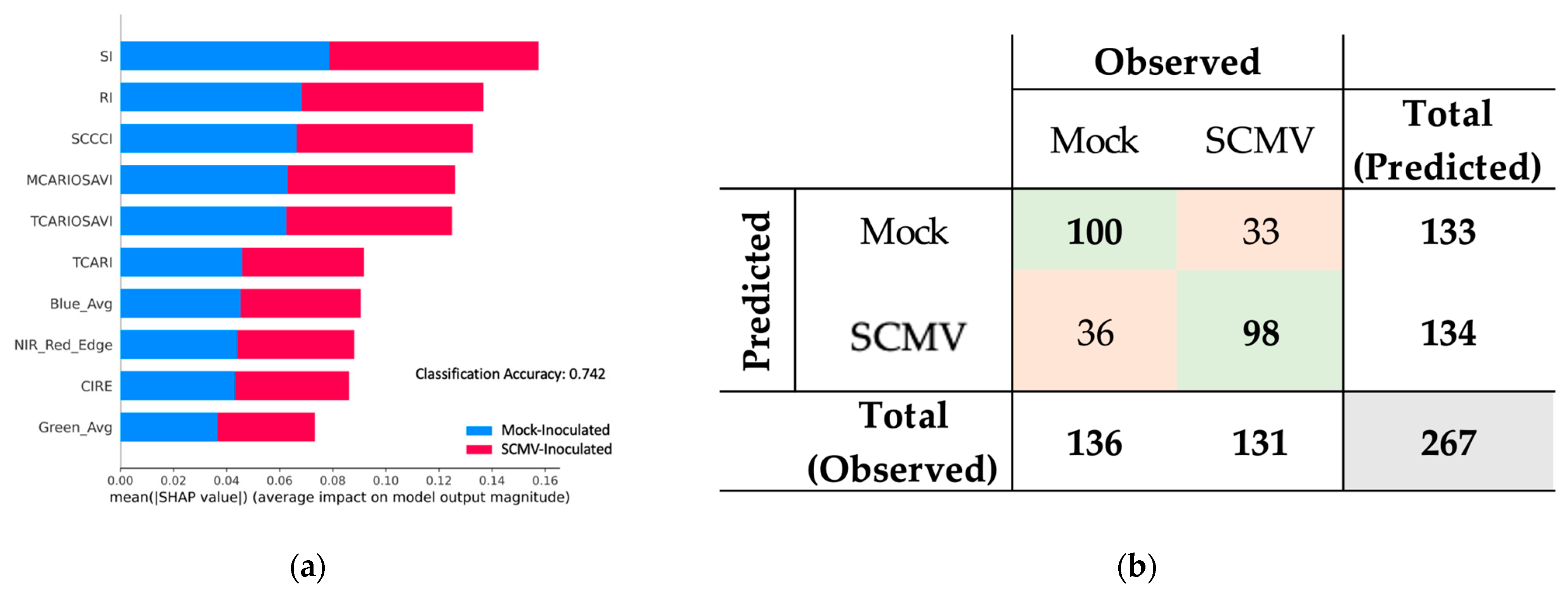
Based on the SHAP analysis of the best-performing SVM classification model for binary SCMV infection prediction, the saturation index (SI) emerged as the feature with the strongest impact on model prediction behavior (Figure 7a). Following SI, TCARI/OSAVI, MCARI/OSAVI, and SCCCI were identified as the most impactful features. The confusion matrix provides more detailed metrics on the SVM model performance with the testing data (Figure 7b). For the test data, the model correctly recalled 100 out of 136 mock-inoculated samples (0.73) and 98 out of 131 SCMV-inoculated samples (0.75). The model misclassified ‘mock-inoculated’ and ‘SCMV-inoculated’ a total of 33 and 36 times, respectively. Precision scores for mock-inoculated and SCMV-inoculated samples were 0.75 and 0.73, respectively.
Figure 7. Bar plot (a) depicts SHAP analysis for SVM classification based on 41 features, using ‘SCMV-inoculated’ and ‘mock-inoculated’ as categories. The confusion matrix (b) displays model performance metrics on a total of 267 test data samples. Numbers in green and red-orange boxes were correctly and incorrectly classified, respectively.
Remotesensing 16 03296 g007

3.8. Model Performance with Additional Features for Disease Incidence Prediction

The addition of thermal and canopy height features resulted in an R2 of 0.225 and an RMSE of 30.73 for the XGBoost regression model trained on both years of data. This is a decreased performance in comparison to an R2 of 0.29 and an RMSE of 29.26 for the equivalent XGBoost model that used 41 multispectrally derived features. Also, the equivalent RFE-simplified XGBoost model with just 14 multispectrally derived features outperformed both models with an R2 of 0.312 and RMSE of 28.39. So, it appears that the additional sensor-based data did not improve model performance and that a reduction in features through RFE slightly improved overall performance.

3.9. Important Indices: SCCCI and SI

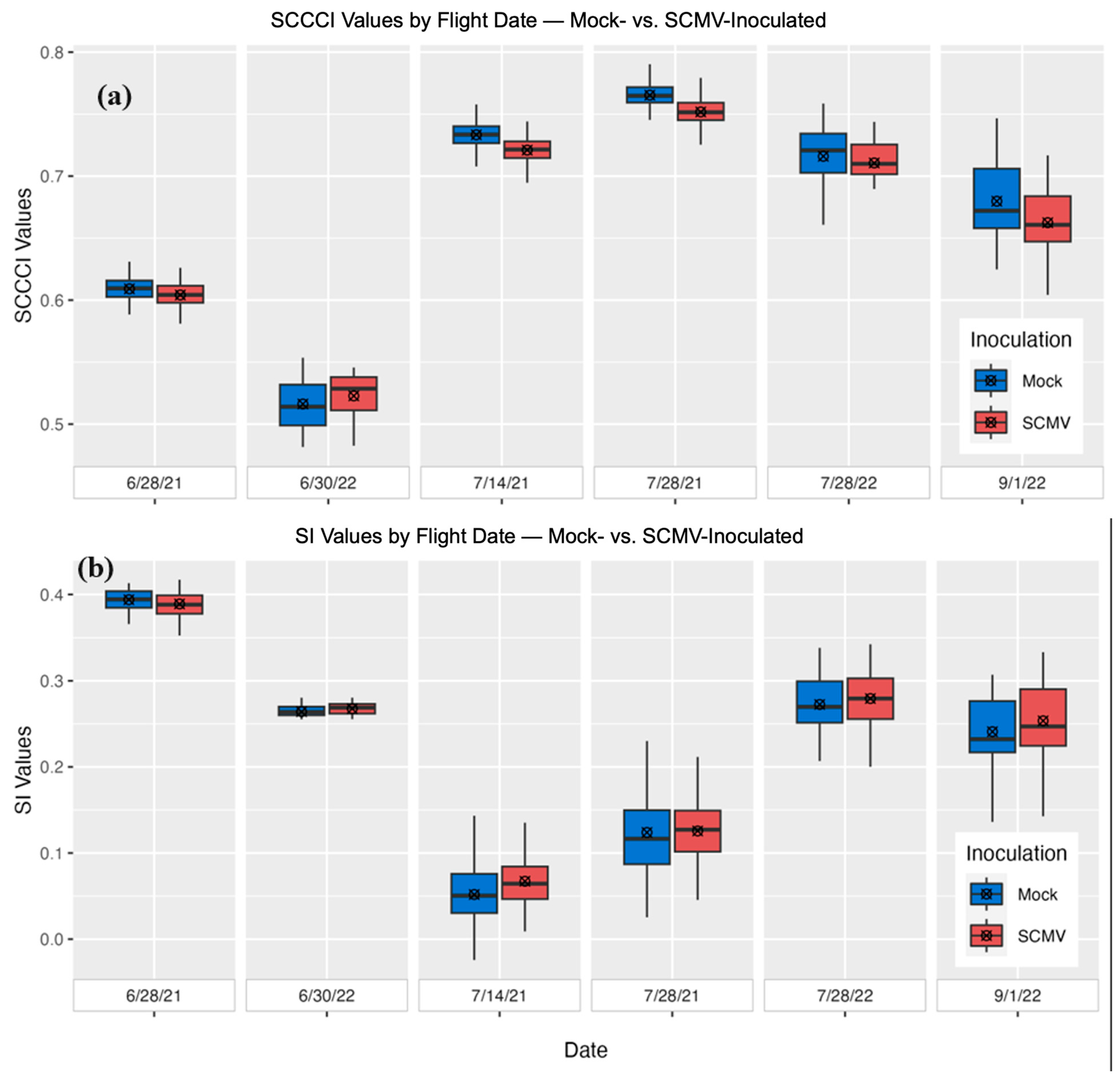
SHAP analysis of both the top-performing XGBoost regression and SVM classification models indicated that SCCCI and SI are two of the most important indices influencing model behavior in SCMV prediction. Further investigation of the SCCCI values across seasonal data indicates that, on average, mock-inoculated samples had consistently higher SCCCI values than SCMV-inoculated samples at all times post-inoculation (Figure 8a). Peak SCCCI values occurred during mid-to-late July and then declined as the season progressed toward harvest. Conversely, SI values exhibited an almost opposite trend (Figure 8b). Following inoculation, the SCMV-inoculated samples had higher SI values compared to mock-inoculated samples, with SI values generally increasing as the season progressed, peaking at the final data collection date.

4. Discussion

4.1. Regression and Classification Modeling

In this study, various modeling approaches were used to investigate the presence and absence of SCMV infection in corn. Given our primary metric for measuring disease incidence was the ‘percentage of infected plants’ per sample plot, our approach can be best viewed as exploratory, with the focus being on variable interpretation and impacts of features on model behavior, as opposed to inferential or predictive analysis.
In this study, treatment plots varied in size across years, making it challenging to interpret the ‘percentage of symptomatic plants’ into an interpretable pixel-wise prediction map. For disease mapping purposes, the classification of disease presence may be more appropriate. Using only multispectral imagery-derived features, the XGBoost regression model for disease incidence percentage had an RMSE value of 29.26, which was reduced to 28.39 after feature reduction via RFE from 41 to 14 features. In contrast, the binary classification SVM model for classifying SCMV inoculation vs. mock inoculation achieved an overall accuracy of 72.9%, with 0.75 recall and 0.73 precision for SCMV inoculation. While the classification model may not provide as much insight into the relationships between spectral features and SCMV disease severity, it could effectively highlight areas suspected to be infected with SCMV. Given that SCMV management largely relies on planting resistant corn varieties, the SVM classification model’s performance may suffice for identifying disease presence across a field. Very precise field locations may not be as necessary as would be the case for a disease that may require the variable-rate precision spraying of pesticides.
Effective models for the prediction of disease incidence were obtained only in 2021 when examining models by year. The models did not capture the variability in the 2022 data very well, which may be attributed to several things. For instance, in 2021, the experimental design had a larger number of hybrid varieties in smaller spatial block sizes, resulting in a larger sample size compared to 2022 (768 observations vs. 120 observations for 2021 and 2022, respectively). This increased diversity of 48 unique hybrid varieties may have resulted in a wider variation in spectral responses due to SCMV inoculation, unlike the limited five hybrid samples in 2022. Generally, larger studies with more samples tend to produce more robust outcomes with reduced margins of error, which may partially explain the stronger fit in the XGBoost regression and SVM classification models for disease incidence in 2021. The lack of significant correlation between disease incidence and spectral variables at Snyder on 28 July 2022 may also be due to the small sample size. Additionally, disease progression at this timestamp might not have yet reached a spectrally significant stage since several significant correlations were noted at the next timestamp.
Furthermore, 2022 included an additional field location not used in the 2021 trials, potentially introducing variation in biotic and abiotic field parameters that could contribute to differences in disease response, thereby impacting model performances. Differences in environmental factors such as temperature, irradiance, and moisture between two years may have also contributed to differences in disease incidence and subsequent spectral responses. While it appeared that both years had similar air temperature and humidity, the 2022 season had higher cumulative rainfall than 2021. For mosaic disease in sugarcane fields, it has been observed that drought conditions and reduced rainfall environments favor the reproduction and activities of aphids, thereby facilitating the spread of mosaic disease [97]. Additionally, excessively hot climates constrain disease transmission, resulting in slower virus proliferation, fewer disease symptoms, and reduced severity of disease outbreaks [97]. This interplay between environmental parameters could contribute to different disease responses and subsequent spectral characteristics between the years.
Lastly, the timing of data collection differed between the years. In 2021, the last disease score date was 12 July 2021, with UAS flight dates on 14 July 2021 and 28 July 2021. In 2022, the last disease score date was 19 July 2022 for Schaffter and 18 July 2022 for Snyder, with UAS flight dates on 28 July 2022 and 1 September 2022. So, all data collection that was used for modeling occurred within 16 days during 2021 and within 46 days during 2022. This discrepancy between plant disease evaluation and UAS flight dates could further explain the weaker model performance in 2022. There may have been continued disease progression that occurred throughout the season and was not comprehensively recorded by the disease incidence scores. Between the recording of disease incidence scores and the last UAS flights (a 16-day gap in 2021 and a 46-day gap in 2022), the SCMV infection may have progressed differently across plots, leading to shifts in disease scores that are not strongly represented in the reported disease scores. Perhaps the disease progressed strongly during this time period for plots that were initially recorded to have low disease scores (a smaller percentage of infected plants). This would render the disease scores less accurate and less informative, such that the ability of the regression model to capture a strong trend in disease scores was diminished. The seemingly better performance of the classification models indicates that the models were more effective at identifying infection presence rather than the severity of the infection (percentage of infected plants).

4.2. Selection of Sensors

Efforts were made to collect temperature data via thermal imagery and canopy height data via LiDAR sensors. However, the addition of these features did not notably enhance model performance for disease incidence prediction. Models built using all the multispectral-derived features (41 bands and indices) performed similarly to the simplified model (14 features). Given these findings, it may not be worth the resources and efforts to collect additional thermal and LiDAR data for SCMV detection purposes as it will require additional sensors and likely additional UAS flights. Moreover, the thermal data exhibited limited correlation with disease incidence, and the collection and processing of thermal data proved challenging, resulting in inconsistent data availability across fields and flight dates. Further investigation into thermal imagery may unveil previously undiscovered trends. However, it is essential to ensure that distinguishable physical characteristics are present in the field when using aerial thermal imagery for remote sensing applications in homogeneous agricultural fields. This will ensure smooth orthomosaic stitching processes.

4.3. Model Performance throughout the Season

This study aimed to compare the performance of models for SCMV detection across time periods and crop growth stages throughout the growing season using 2021 and 2022 data. Each year involved three data collection dates for UAS flights, with the first flight in June occurring before SCMV systemic infection. Thus, the June dates for both years exhibited poor predictive ability, leading to their exclusion from the final model building. Unfortunately, this resulted in less data available for modeling, suggesting potential benefits from additional flights post-inoculation.
In 2021, the performance of models for disease incidence prediction gradually improved throughout the season, whereas the effectiveness of disease prediction in 2022 generally lagged behind, although it did show improvement as the growing season progressed. This trend aligns with the progression of infection and increasing plant physiological symptoms. However, this trend may not hold true for MDM, as many hybrids lack visible symptoms at later growth stages. Based on these findings, aerial imagery scouting for SCMV infection during the latter half of July or potentially later into August may prove most effective and economical. Generating a predicted disease presence map could also facilitate targeted on-ground investigation, enabling effective disease management strategies for subsequent seasons, such as crop rotation or improved weed control, to mitigate virus overwintering and its aphid vector.

4.4. Spectral Features and Model Behavior

4.4.1. Spectral Bands

SCMV infection can alter plant pigment and canopy structure, influencing spectral reflectance values. In 2021, SCMV-inoculated plants displayed significant differences in red, red-edge, and NIR bands compared to mock-inoculated plants. SCMV-inoculated plants generally had higher reflectance in the visible and red-edge bands but lower reflectance in the NIR bands (Figure S1). These changes align with expected variations in spectral profiles in healthy and unhealthy vegetation [98,99].
Using chlorophyll content as a positive proxy for healthy vegetation, it is expected that healthier vegetation will have a higher absorption (lower reflectance) in the blue (peaks at 430 and 453 nm for chlorophyll a) and red (peaks at 642 and 662nm for chlorophyll b) bands and a lower absorption in green (in the 500–600 nm) bands as compared to unhealthy plants that lack the equivalent amount of chlorophyll [99,100,101]. SCMV infection causes initial chlorotic spotting, streaking, mosaicking, and the eventual progressive yellowing of leaves, which may explain the average differences found in the visible reflectance values. The higher reflectance values observed in SCMV-inoculated plots for both blue and red bands suggest an impact on chlorophyll content due to SCMV infection. This finding is supported by the significant differences observed in the red band, suggesting a stronger influence on chlorophyll b content by SCMV infection, leading to reduced red reflectance.
The red-edge portion (680–740 nm) of the spectrum serves as a transition zone between the red and NIR spectra where reflectance shifts from being primarily influenced by photosynthetic pigments (chlorophyll) to vegetation structural properties [102,103,104]. Red-edge radiation penetrates deeper into crop canopies than visible light, making red-edge-based indices less susceptible to chlorophyll saturations with increasing values of the leaf area index later in the growing season unlike NDVI [104,105]. Furthermore, the red-edge position typically shifts towards longer wavelengths in healthy plants, while it shifts towards shorter wavelengths in diseased plants [103,106]. In this study, SCMV-inoculated plants exhibited higher average red-edge reflectance across both fields and years, suggesting potential stress from disease infection. However, confirming this speculation is challenging due to the use of broadband multispectral images in the analyses.

4.4.2. Vegetation Indices and Feature Importance

SCCCI was identified as the most impactful feature for model behavior in both XGBoost Regression and SVM classification models (Figure 6a). SCCCI, derived from NDRE divided by NDVI, integrates NIR, red, and red-edge bands. Originally proposed as a red-edge index for cotton, SCCCI offers robustness compared to NDVI, particularly in avoiding early-season saturation [68,107,108]. Similarly, TCARI/OSAVI was ranked high in both regression and classification analyses. These two indices, along with MCARI/OSAVI, also show promise in explaining corn’s nitrogen status using multispectral aerial imagery [76,108]. The prominence of SCCCI in disease incidence prediction suggests that SCMV-infected plants may exhibit reduced chlorophyll or photosynthetic pigment production across the canopy, while the leaf area index and vegetation cover remain relatively unaffected. This indicates that SCMV infection primarily impacts pigment performance rather than the structural integrity of the plant from an aerial imagery perspective. While SCMV infection may not drastically affect plant structure, it can lead to stunting or increased bushiness. LiDAR-derived canopy heights on 28 July 2022 did not show significant stunting between inoculated and mock-inoculated plants, but visible height differences in August/September suggest some stunting due to SCMV infection.
The saturation index (SI), also known as the normalized pigment chlorophyll index (NPCI), utilizes the red and blue regions and emerged as the most important feature for SCMV infection classification by SVM and the second most crucial feature for disease incidence prediction by XGBoost according to SHAP analyses. SI was originally designed to assess the carotenoid-to-chlorophyll ratio and is higher in nitrogen-limited leaves and inversely correlated with chlorophyll content [75]. The ratio between carotenoids and chlorophyll a typically decreases as plants grow and then increases as they senesce [109,110].
Carotenoids, with their photoprotective role in photosynthesis [111], contribute similarly to chlorophyll in visible absorption for wavelengths shorter than green [75]. However, they do not absorb as strongly in the red region as chlorophyll does. SI may, therefore, relate to the proportions of total photosynthetic pigments to chlorophyll proportions, influenced by nitrogen limitations or the protective effects of carotenoids [75,111]. The SHAP analysis of the disease incidence model indicates an almost inverse relationship of SI on model prediction compared to SCCCI. High SI values suggest increased disease incidence prediction, potentially indicating a discrepancy in carotenoid to chlorophyll content in heavily SCMV-infected plants [111]. However, these observations remain speculative without quantified estimations of photosynthetic pigment content levels in SCMV-inoculated and mock-inoculated plants. Notably, SI can be calculated using just an RGB camera, making it a potentially more cost-efficient method for predicting disease incidence in corn compared to using a multispectral camera.

4.5. Limitations and Steps Forward

The study revealed insights into the spectral characteristics of SCMV infection and proposed a methodology for its detection using multispectral data. However, variations in model performance between years suggested limited generalizability to new data. Specifically, the performance of the XGBoost regression model trained on 2021 data and tested with 2022 data highlighted this issue. This could be attributed to the limited dataset, particularly the lack of extensive 2022 data. This limitation can be addressed through the further collection of annotated multispectral imagery and ground truth data covering a range of field sites, environmental conditions, inoculation rates, corn hybrid varieties, crop growth stages, and management practices. This helps to build a larger, more diverse dataset, ultimately enhancing model performance and transferability to new fields and new seasons. Additionally, we had success using sequential model-based optimization (Hyperopt) to finalize model hyperparameters and then using recursive feature elimination to minimize the included features for XGBoost regression modeling. However, the additional fine-tuning of all the models with more data would confirm that XGBoost is indeed the best model and would also likely improve predictive accuracy.
The use of field scouting and disease incidence percentage as infection metrics to correlate with spectral properties can introduce human subjectivity and potential errors, which might have influenced the modeling process. Although these methods are practical and efficient, reflecting real-world SCMV scouting practices, obtaining quantitative estimates of virus titer through serological and molecular testing for individual plants could offer a deeper understanding of spectral relationships. However, these lab-based approaches are costly and time-consuming. Using the average disease incidence value and the average reflectance values of each hybrid plot has limitations regarding the precise mapping of disease incidence. For instance, some of the plants within a specific inoculated plot may be relatively healthy (e.g., they may have a high NDVI value) compared to other plants within the same plot, and, thus, the detection of disease presence or severity may be reduced or understated by averaging. Deriving a standard deviation from zonal statistics as a feature may also yield insightful results. However, as stated, given that SCMV treatment largely relies on planting resistant maize varieties during the next season, the identification of disease presence from means within a general area of a field can still be very informative for management decisions.
While limited observations of LiDAR and thermal imagery did not enhance model performance, exploring them further by incorporating data collected at various stages of SCMV infection may be valuable. To avoid concerns with the stitching of thermal imagery, it is suggested that special consideration be given to ground control points and georeferencing techniques specific to thermal imagery collection. Quantifying chlorophyll and pigment content through leaf tissues or plant sap analysis may elucidate the biochemical and physiological responses of corn to SCMV, which may then provide clarity on spectral indices’ effectiveness for SCMV prediction. Additionally, hyperspectral imagery may offer a higher-resolution understanding of SCMV’s impact on spectral characteristics and aid in disease identification.

5. Conclusions

This study primarily explores the potential of using UAS multispectral imagery for the detection of SCMV infection in corn fields using data collected over the 2021 and 2022 growing seasons at two farms in Ohio, USA. Field experiments with randomized block designs were implemented such that it was known which plots of each field were noninfected or infected with SCMV. Using the multispectral orthomosaic images, mean pixel reflectance values were calculated for each of the five spectral bands within each individual sample treatment plot. On average, SCMV-inoculated plants had higher reflectance values for blue, green, red, and red-edge bands and lower reflectance for near-infrared bands as compared to mock-inoculated samples. Machine learning algorithms were used for the exploratory analysis and predictive modeling of disease incidence percentage as regression and disease presence as a binary classification. For data aggregated from both years, an XGBoost model using just 14 multispectral image-derived features determined using recursive feature elimination performed best for ‘disease incidence’ prediction with an R2 of 0.312 and an RMSE of 28.39. The SVM model was the best classification model for predicting SCMV disease presence with an accuracy of 0.729. A SHAP analysis demonstrated that the SCCCI, SI, and TCARI/OSAVI vegetation indices were generally the most impactful on model performance for the prediction and detection of SCMV in corn. A larger aerial multispectral and thermal image dataset is needed to build models that transfer the high performance of SCMV detection to additional unseen data and new fields. The methodology developed in this study demonstrates the potential for the development of a tool for farmers that may facilitate the precise identification and mapping of SCMV infection in corn.

Supplementary Materials

The following supporting information can be downloaded at https://www.mdpi.com/article/10.3390/rs16173296/s1: Figure S1: Boxplots displaying the comparison of the average reflectance values for each of the spectral bands for SCMV-inoculated and mock-inoculated corn plants; Table S1: Hyperparameters Spaces Explore; Table S2: Significant Pearson r Correlations.

Author Contributions

Conceptualization, S.K. and E.W.O.; methodology, N.B., E.W.O., M.W.J., K.K. and S.K.; software, N.B.; validation, N.B.; formal analysis, N.B.; investigation, N.B., E.W.O. and S.K.; resources, S.K., E.W.O. and M.W.J.; data curation, N.B. and K.K.; writing—original draft preparation, N.B.; writing—review and editing, N.B., E.W.O., S.K., M.W.J. and K.K.; visualization, Bever, N.; supervision, S.K.; project administration, S.K.; funding acquisition, S.K. and E.W.O. All authors have read and agreed to the published version of the manuscript.

Funding

This research was funded in part by USDA-ARS (58-5082-2-006), OSU Graduate School Fellowship, and NRT EmPowerment Fellowship.

Data Availability Statement

The data used in this study can be made available upon request.

Acknowledgments

We would like to thank Mark Bolin for collecting the UAS-based LiDAR data and Peter Thomison, Rich Minyo, and industry participants for providing hybrid seeds. We also thank Chris Nacci, Lynn Ault, Bob Napier, and Matthew Lowe for their assistance in the field.

Conflicts of Interest

The authors declare no conflicts of interest.

References

  1. García-Lara, S.; Serna-Saldivar, S.O. Corn History and Culture (Third Edition). Corn Chem. Technol. Third Ed. 2019, 1–18. [Google Scholar] [CrossRef]
  2. Erenstein, O.; Jaleta, M.; Sonder, K.; Mottaleb, K.; Prasanna, B.M. Global maize production, consumption and trade: Trends and R&D implications. Food Secur. 2022, 14, 1295–1319. [Google Scholar] [CrossRef]
  3. Savary, S.; Willocquet, L.; Pethybridge, S.J.; Esker, P.; McRoberts, N.; Nelson, A. The global burden of pathogens and pests on major food crops. Nat. Ecol. Evol. 2019, 3, 430–439. [Google Scholar] [CrossRef]
  4. Zambrano, J.L.; Stewart, L.R.; Paul, P.A. Maize Dwarf Mosaic of Maize. Ohio State University Extension. 2016. Available online: https://ohioline.osu.edu/factsheet/plpath-cer-09 (accessed on 5 May 2023).
  5. Shukla, D.D.; Tosic, M.; Jilka, J.; Ford, R.E.; Toler, R.W.; Langham, M.A.C. Taxonomy of potyviruses infecting maize, sorghum and sugarcane in Australia and the United States as determined by reactivities of polyclonal antibodies directed towards virus-specific N-termini of coat proteins. Phytopathology 1989, 79, 223–229. [Google Scholar] [CrossRef]
  6. Tosic, M.; Ford, R.E.; Shukla, D.D.; Jilka, J. Differentiation of Sugarcane, Maize dwarf, Johnsongrass, and Sorghum mosaic viruses based on reactions of oat and some sorghum cultivars. Plant Dis. 1990, 74, 549–552. [Google Scholar] [CrossRef]
  7. Frenkel, M.J.; Jilka, J.M.; McKern, N.M.; Strike, P.M.; Clark, J.M., Jr.; Shukla, D.D.; Ward, C.W. Unexpected sequence diversity in the amino-terminal ends of the coat proteins of strains of sugarcane mosaic virus. J. Gen. Virol. 1991, 72, 237–242. [Google Scholar] [CrossRef] [PubMed]
  8. Gao, B.; Cui, X.-W.; Li, X.-D.; Zhang, C.-Q.; Miao, H.-Q. Complete genomic sequence analysis of a highly virulent isolate revealed a novel strain of Sugarcane mosaic virus. Virus Genes 2011, 43, 390–397. [Google Scholar] [CrossRef]
  9. Viswanathan, R.; Karuppaiah, R.; Balamuralikrishnan, M. Identification of new variants of SCMV causing sugarcane mosaic in India and assessing their genetic diversity in relation to SCMV type strains. Virus Genes 2009, 39, 375–386. [Google Scholar] [CrossRef]
  10. Niblett, C.; Claflin, L. Corn lethal necrosis—A new virus disease of corn in Kansas. Plant Dis. Bull. 1978, 62, 15. [Google Scholar]
  11. Stewart, L.R.; Willie, K.; Wijeratne, S.; Redinbaugh, M.G.; Massawe, D.; Niblett, C.L.; Kiggundu, A.; Asiimwe, T. Johnsongrass mosaic virus contributes to maize lethal necrosis in East Africa. Plant Dis. 2017, 101, 1455–1462. [Google Scholar] [CrossRef] [PubMed]
  12. Redinbaugh, M.G.; Stewart, L.R. Maize lethal necrosis: An emerging, synergistic viral disease. Annu. Rev. Virol. 2018, 5, 301–322. [Google Scholar] [CrossRef] [PubMed]
  13. Ohlson, E.W.; Redinbaugh, M.G.; Jones, M.W. Mapping maize chlorotic mottle virus tolerance loci in the Maize 282 Association Panel. Crop Sci. 2022, 62, 1497–1510. [Google Scholar] [CrossRef]
  14. Wu, L.; Zu, X.; Wang, S.; Chen, Y. Sugarcane mosaic virus—Long history but still a threat to industry. Crop Prot. 2012, 42, 74–78. [Google Scholar] [CrossRef]
  15. Xu, D.L.; Park, J.W.; Mirkov, T.E.; Zhou, G.H. Viruses causing mosaic disease in sugarcane and their genetic diversity in southern China. Arch. Virol. 2008, 153, 1031–1039. [Google Scholar] [CrossRef]
  16. Fuchs, E.; Grüntzig, M. Influence of sugarcane mosaic virus (SCMV) and maize dwarf mosaic virus (MDMV) on the growth and yield of two maize varieties. J. Plant Dis. Prot. 1995, 102, 44–50. Available online: http://www.jstor.org/stable/43386365 (accessed on 1 May 2023).
  17. Janson, B.F.; Williams, L.E.; Findley, W.R.; Dollinger, E.J.; Ellett, C.W. Maize dwarf mosaic: New corn virus disease in Ohio. 1965. Available online: https://www.cabidigitallibrary.org/doi/full/10.5555/19641101624 (accessed on 21 April 2023).
  18. Gustafson, T.J.; de Leon, N.; Kaeppler, S.M.; Tracy, W.F. Genetic analysis of sugarcane mosaic virus resistance in the wisconsin diversity panel of maize. Crop Sci. 2018, 58, 1853–1865. [Google Scholar] [CrossRef]
  19. Meyer, M.D.; Pataky, J.K. Increased severity of foliar diseases of sweet corn infected with maize dwarf mosaic and sugarcane mosaic viruses. Plant Dis. 2010, 94, 1093–1099. [Google Scholar] [CrossRef]
  20. Jones, M.W.; Ohlson, E.W. Susceptibility and yield response of commercial corn hybrids to maize dwarf mosaic disease. Plant Dis. 2024, 108, 1786–1792. [Google Scholar] [CrossRef]
  21. Kerns, M.R.; Pataky, J.K. Reactions of Sweet Corn Hybrids with Resistance to Maize Dwarf Mosaic. Plant Dis. 1997, 81, 460–464. [Google Scholar] [CrossRef]
  22. Shahi, T.B.; Xu, C.-Y.; Neupane, A.; Guo, W. Recent advances in crop disease detection using UAV and deep learning techniques. Remote Sens. 2023, 15, 2450. [Google Scholar] [CrossRef]
  23. Zhang, J.; Huang, Y.; Pu, R.; Gonzalez-Moreno, P.; Yuan, L.; Wu, K.; Huang, W. Monitoring plant diseases and pests through remote sensing technology: A review. Comput. Electron. Agric. 2019, 165, 104943. Available online: https://www.sciencedirect.com/science/article/pii/S016816991930290X (accessed on 2 May 2023). [CrossRef]
  24. Tsouros, D.C.; Bibi, S.; Sarigiannidis, P.G. A review on UAV-based applications for precision agriculture. Information 2019, 10, 349. [Google Scholar] [CrossRef]
  25. Khanal, S.; KC, K.; Fulton, J.; Shearer, S.; Ozkan, E. Remote Sensing in Agriculture (Challenges and Opportunities). Remote Sens. 2020, 12, 3783. [Google Scholar] [CrossRef]
  26. Chakravarthy, A.K. Innovative Pest Management Approaches for the 21st Century: Harnessing Automated Unmanned Technologies; Springer Nature: New York, NY, USA, 2020; pp. 255–272. [Google Scholar]
  27. Bannari, A.; Morin, D.; Bonn, F.; Huete, A.R. A review of vegetation indices. Remote Sens. Rev. 1995, 13, 95–120. [Google Scholar] [CrossRef]
  28. Huang, S.; Tang, L.; Hupy, J.P.; Wang, Y.; Shao, G. A commentary review on the use of normalized difference vegetation index (NDVI) in the era of popular remote sensing. J. For. Res. 2021, 32, 2719. [Google Scholar] [CrossRef]
  29. Antolínez García, A.; Cáceres Campana, J.W. Identification of pathogens in corn using near-infrared UAV imagery and deep learning. Precis. Agric. 2023, 24, 783–806. [Google Scholar] [CrossRef]
  30. Butcher, G. Tour of the Electromagnetic Spectrum; Government Printing Office: Washington, DC, USA, 2016. [Google Scholar]
  31. Barbedo, J.G.A. A review on the main challenges in automatic plant disease identification based on visible range images. Biosyst. Eng. 2016, 144, 52–60. [Google Scholar] [CrossRef]
  32. Mohanty, S.P.; Hughes, D.P.; Salathé, M. Using deep learning for image-based plant disease detection. Front. Plant Sci. 2016, 7, 1419. [Google Scholar] [CrossRef]
  33. Moriya, E.A.S.; Imai, N.N.; Tommaselli, A.M.G.; Miyoshi, G.T. Mapping Mosaic Virus in Sugarcane Based on Hyperspectral Images. IEEE J. Sel. Top. Appl. Earth Obs. Remote Sens. 2017, 10, 740–748. [Google Scholar] [CrossRef]
  34. Viswanathan, R.; Rao, G.P. Disease Scenario and Management of Major Sugarcane Diseases in India. Sugar Tech 2011, 13, 336–353. [Google Scholar] [CrossRef]
  35. Gazala, I.F.S.; Sahoo, R.N.; Pandey, R.; Mandal, B.; Gupta, V.K.; Singh, R.; Sinha, P. Spectral reflectance pattern in soybean for assessing yellow mosaic disease. Indian J. Virol. 2013, 24, 242–249. [Google Scholar] [CrossRef]
  36. Mirik, M.; Jones, D.C.; Price, J.A.; Workneh, F.; Ansley, R.J.; Rush, C.M. Satellite remote sensing of wheat infected by Wheat streak mosaic virus. Plant Dis. 2011, 95, 4–12. [Google Scholar] [CrossRef]
  37. Prabhakar, M.; Prasad, Y.G.; Desai, S.; Thirupathi, M.; Gopika, K.; Rao, G.R.; Venkateswarlu, B. Hyperspectral remote sensing of yellow mosaic severity and associated pigment losses in Vigna mungo using multinomial logistic regression models. Crop Prot. 2013, 45, 132–140. [Google Scholar] [CrossRef]
  38. Luo, L.; Chang, Q.; Wang, Q.; Huang, Y. Identification and severity monitoring of maize dwarf mosaic virus infection based on hyperspectral measurements. Remote Sens. 2021, 13, 4560. [Google Scholar] [CrossRef]
  39. Ausmus, B.S.; Hilty, J.W. Reflectance studies of healthy, maize dwarf mosaic virus-infected, and Helminthosporium maydis-infected corn leaves. Remote Sens. Environ. 1971, 2, 77–81. [Google Scholar] [CrossRef]
  40. Dhau, I.; Adam, E.; Ayisi, K.K.; Mutanga, O. Detection and mapping of maize streak virus using RapidEye satellite imagery. Geocarto Int. 2019, 34, 856–866. [Google Scholar] [CrossRef]
  41. Dhau, I.; Dube, T.; Mushore, T.D. Examining the prospects of sentinel-2 multispectral data in detecting and mapping maize streak virus severity in smallholder Ofcolaco farms, South Africa. Geocarto Int. 2021, 36, 1873–1883. [Google Scholar] [CrossRef]
  42. Dhau, I.; Adam, E.; Mutanga, O.; Ayisi, K.K. Detecting the severity of maize streak virus infestations in maize crop using in situ hyperspectral data. Trans. R. Soc. S. Africa 2018, 73, 8–15. [Google Scholar] [CrossRef]
  43. Chen, S.; Zhang, K.; Wu, S.; Tang, Z.; Zhao, Y.; Sun, Y.; Shi, Z. A Weakly Supervised Approach for Disease Segmentation of Maize Northern Leaf Blight from UAV Images. Drones 2023, 7, 173. [Google Scholar] [CrossRef]
  44. Garg, K.; Bhugra, S.; Lall, B. Automatic quantification of plant disease from field image data using deep learning. In Proceedings of the 2021 IEEE Winter Conference on Applications of Computer Vision, WACV 2021, Waikoloa, HI, USA, 3–8 January 2021; pp. 1964–1971. [Google Scholar] [CrossRef]
  45. Wu, H.; Wiesner-Hanks, T.; Stewart, E.L.; DeChant, C.; Kaczmar, N.; Gore, M.A.; Nelson, R.J.; Lipson, H. Autonomous Detection of Plant Disease Symptoms Directly from Aerial Imagery. Plant Phenome J. 2019, 2, 1–9. [Google Scholar] [CrossRef]
  46. Dhau, I.; Adam, E.; Mutanga, O.; Ayisi, K.; Abdel-Rahman, E.M.; Odindi, J.; Masocha, M. Testing the capability of spectral resolution of the new multispectral sensors on detecting the severity of grey leaf spot disease in maize crop. Geocarto Int. 2018, 33, 1223–1236. [Google Scholar] [CrossRef]
  47. Loladze, A.; Rodrigues, F.A.; Toledo, F.; Vicente, F.S.; Gérard, B.; Boddupalli, M.P. Application of remote sensing for phenotyping tar spot complex resistance in maize. Front. Plant Sci. 2019, 10, 552. [Google Scholar] [CrossRef]
  48. Pix4D, Version 4.2.27; Pix4D Mapper Photogrammetry Software: Lausanne, Switzerland.
  49. ESRI. ArcGIS Pro; Environmental Systems Research Institute: Redlands, CA, USA, 2023. [Google Scholar]
  50. R Core Team RF for SC. R: A Language and Environment; R Core Team: Vienna, Austria, 2019; Available online: https://www.r-project.org/ (accessed on 3 May 2023).
  51. Parker, T.A.; Palkovic, A.; Gepts, P. Determining the genetic control of common bean early-growth rate using unmanned aerial vehicles. Remote Sens. 2020, 12, 1748. [Google Scholar] [CrossRef]
  52. Woebbecke, D.M.; Meyer, G.E.; Von Bargen, K.; Mortensen, D.A. Color Indices for Weed Identification Under Various Soil, Residue, and Lighting Conditions. Trans. ASAE 1995, 38, 259–269. Available online: https://elibrary.asabe.org/azdez.asp?JID=&AID=27838&CID=t1995&v=38&i=1&T=1 (accessed on 3 May 2023). [CrossRef]
  53. Girardeau-Montaut, D. CloudCompare; EDF R&D Telecom ParisTech: Paris, France, 2016; Available online: https://www.danielgm.net/cc/ (accessed on 4 January 2023).
  54. Ray, S.S.; Singh, J.P.; Das, G.; Panigrahy, S.; Group, A.R.; Centre, S.A.; Potato, C. Use of high resolution remote sensing data for generating site-specific soil mangement plan. Red 2004, 550, 727. [Google Scholar]
  55. Gitelson, A.A.; Vina, A.; Arkebauer, T.J.; Rundquist, D.C.; Keydan, G.; Leavitt, B. Remote estimation of leaf area index and green leaf biomass in maize canopies. Geophys. Res. Lett. 2003, 30, 4–7. [Google Scholar] [CrossRef]
  56. Hunt, E.R.; Doraiswamy, P.C.; McMurtrey, J.E.; Daughtry, C.S.T.; Perry, E.M.; Akhmedov, B. A visible band index for remote sensing leaf chlorophyll content at the Canopy scale. Int. J. Appl. Earth Obs. Geoinf. 2012, 21, 103–112. [Google Scholar] [CrossRef]
  57. Huete, A.; Didan, K.; Miura, T.; Rodriguez, E.P.; Gao, X.; Ferreira, L.G. Overview of the radiometric and biophysical performance of the MODIS vegetation indices. Remote Sens. Environ. 2002, 82, 195–213. [Google Scholar] [CrossRef]
  58. Gitelson, A.A.; Kaufman, Y.J.; Merzlyak, M.N. Use of a green channel in remote sensing of global vegetation from EOS-MODIS. Remote Sens. Environ. 1996, 58, 289–298. [Google Scholar] [CrossRef]
  59. Gitelson, A.A.; Merzlyak, M.N. Remote sensing of chlorophyll concentration in higher plant leaves. Adv. Sp. Res. 1998, 22, 689–692. [Google Scholar] [CrossRef]
  60. Gitelson, A.A. Wide Dynamic Range Vegetation Index for Remote Quantification of Biophysical Characteristics of Vegetation. J. Plant Physiol. 2004, 161, 165–173. [Google Scholar] [CrossRef]
  61. Junior, C.K.; Guimarães, A.M.; Caires, E.F. Use of active canopy sensors to discriminate wheat response to nitrogen fertilization under no-tillage. Eng. Agric. 2016, 36, 886. [Google Scholar] [CrossRef]
  62. Portz, G.; Molin, J.P.; Jasper, J. Active crop sensor to detect variability of nitrogen supply and biomass on sugarcane fields. Precis. Agric. 2012, 13, 33–44. [Google Scholar] [CrossRef]
  63. Banerjee, B.P.; Spangenberg, G.; Kant, S. Fusion of spectral and structural information from aerial images for improved biomass estimation. Remote Sens. 2020, 12, 3164. [Google Scholar] [CrossRef]
  64. Haboudane, D.; Miller, J.R.; Pattey, E.; Zarco-Tejada, P.J.; Strachan, I.B. Hyperspectral vegetation indices and novel algorithms for predicting green LAI of crop canopies: Modeling and validation in the context of precision agriculture. Remote Sens. Environ. 2004, 90, 337–352. [Google Scholar] [CrossRef]
  65. Rondeaux, G.; Steven, M.; Baret, F. Optimization of soil-adjusted vegetation indices. Remote Sens. Environ. 1996, 55, 95–107. [Google Scholar] [CrossRef]
  66. Qi, J.; Chehbouni, A.; Huete, A.R.; Kerr, Y.H.; Sorooshian, S. A modified soil adjusted vegetation index. Remote Sens. Environ. 1994, 48, 119–126. [Google Scholar] [CrossRef]
  67. Chen, J.M. Evaluation of vegetation indices and a modified simple ratio for boreal applications. Can. J. Remote Sens. 1996, 22, 229–242. [Google Scholar] [CrossRef]
  68. Barnes, E.M.; Clarke, T.R.; Richards, S.E.; Colaizzi, P.D.; Haberland, J.; Kostrzewski, M.; Walker, P.; Choi, C.; Riley, E.; Thompson, T.; et al. Coincident detection of crop water stress, nitrogen status and canopy density using ground based multispectral data. In Proceedings of the Fifth International Conference on Precision Agriculture, Bloomington, MN, USA, 19 July 2000; Volume 1619. [Google Scholar]
  69. Rouse, J.W., Jr.; Haas, R.H.; Deering, D.W.; Schell, J.A.; Harlan, J.C. Monitoring the Vernal Advancement and Retrogradation (Green Wave Effect) of Natural Vegetation; NASA/GSFCT Type III Final Report, 371; NASA: Washington, DC, USA, 1974. [Google Scholar]
  70. Gitelson, A.A.; Kaufman, Y.J.; Stark, R.; Rundquist, D. Novel algorithms for remote estimation of vegetation fraction. Remote Sens. Environ. 2002, 80, 76–87. [Google Scholar] [CrossRef]
  71. Ramoelo, A.; Skidmore, A.K.; Cho, M.A.; Schlerf, M.; Mathieu, R.; Heitkönig, I.M.A. Regional estimation of savanna grass nitrogen using the red-edge band of the spaceborne rapideye sensor. Int. J. Appl. Earth Obs. Geoinf. 2012, 19, 151–162. [Google Scholar] [CrossRef]
  72. Roujean, J.L.; Breon, F.M. Estimating PAR absorbed by vegetation from bidirectional reflectance measurements. Remote Sens. Environ. 1995, 51, 375–384. [Google Scholar] [CrossRef]
  73. Huete, A.R. A soil-adjusted vegetation index (SAVI). Remote Sens. Environ. 1998, 25, 295–309. [Google Scholar] [CrossRef]
  74. Raper, T.B.; Varco, J.J. Canopy-scale wavelength and vegetative index sensitivities to cotton growth parameters and nitrogen status. Precis. Agric. 2015, 16, 62–76. [Google Scholar] [CrossRef]
  75. Peñuelas, J.; Gamon, J.A.; Fredeen, A.L.; Merino, J.; Field, C.B. Reflectance indices associated with physiological changes in nitrogen- and water-limited sunflower leaves. Remote Sens. Environ. 1994, 48, 135–146. [Google Scholar] [CrossRef]
  76. Haboudane, D.; Miller, J.R.; Tremblay, N.; Zarco-Tejada, P.J.; Dextraze, L. Integrated narrow-band vegetation indices for prediction of crop chlorophyll content for application to precision agriculture. Remote Sens. Environ. 2002, 81, 416–426. [Google Scholar] [CrossRef]
  77. Revelle, W.; Revelle, M.W. Package ‘psych’. Compr. R Arch. Netw. 2015, 337, 161–165. [Google Scholar]
  78. Kruskal, W.H.; Wallis, W.A. Use of ranks in one-criterion variance analysis. J. Am. Stat. Assoc. 1952, 47, 583–621. [Google Scholar] [CrossRef]
  79. McDonald, G.C. Ridge regression. Wiley Interdiscip. Rev. Comput. Stat. 2009, 1, 93–100. Available online: https://onlinelibrary.wiley.com/doi/full/10.1002/wics.14 (accessed on 3 May 2023). [CrossRef]
  80. Hearst, M.A.; Dumais, S.T.; Osuna, E.; Platt, J.; Scholkopf, B. Support vector machines. IEEE Intell. Syst. Their Appl. 1998, 13, 18–28. [Google Scholar] [CrossRef]
  81. Breiman, L. Random forests. Mach. Learn. 2001, 45, 5–32. Available online: https://link.springer.com/article/10.1023/A:1010933404324 (accessed on 3 May 2023). [CrossRef]
  82. Chen, T.; Guestrin, C. XGBoost: A scalable tree boosting system. In Proceedings of the 22nd ACM SIGKDD International Conference on Knowledge Discovery and Data Mining, San Francisco, CA, USA, 13–17 August 2016; pp. 785–794. [Google Scholar] [CrossRef]
  83. Ballabio, C.; Sterlacchini, S. Support vector machines for landslide susceptibility mapping: The Staffora River Basin case study, Italy. Math. Geosci. 2012, 44, 47–70. [Google Scholar] [CrossRef]
  84. Triscowati, D.W.; Sartono, B.; Kurnia, A.; Domiri, D.D.; Wijayanto, A.W. Multitemporal remote sensing data for classification of food crops plant phase using supervised random forest. In Proceedings of the Sixth Geoinformation Science Symposium, Yogyakarta, Indonesia, 26–27 August 2019; Volume 11311, p. 1131102. [Google Scholar]
  85. Fan, J.; Zhou, J.; Wang, B.; de Leon, N.; Kaeppler, S.M.; Lima, D.C.; Zhang, Z. Estimation of Maize Yield and Flowering Time Using Multi-Temporal UAV-Based Hyperspectral Data. Remote Sens. 2022, 14, 3052. [Google Scholar] [CrossRef]
  86. Hoerl, A.E.; Kennard, R.W. Ridge Regression: Biased Estimation for Nonorthogonal Problems. Technometrics 1970, 12, 55–67. Available online: https://www.tandfonline.com/doi/abs/10.1080/00401706.1970.10488634 (accessed on 3 May 2023). [CrossRef]
  87. Awad, M.; Khanna, R. Support Vector Regression. In Efficient Learning Machines; Apress: Berkeley, CA, USA, 2015; pp. 67–80. Available online: https://link.springer.com/chapter/10.1007/978-1-4302-5990-9_4 (accessed on 3 May 2023).
  88. Smola, A.J.; Schölkopf, B. A tutorial on support vector regression. Stat. Comput. 2004, 14, 199–222. Available online: https://link.springer.com/article/10.1023/B:STCO.0000035301.49549.88 (accessed on 3 May 2023). [CrossRef]
  89. Drucker, H.; Burges, C.J.C.; Kaufman, L.; Smola, A.; Vapoik, V. Support Vector Regression Machines. Adv. Neural Inf. Process. Syst. 1996, 9, 155–161. [Google Scholar]
  90. Cutler, A.; Cutler, D.R.; Stevens, J.R. Random Forests. In Ensemble Machine Learning; Springer: New York, NY, USA, 2012; pp. 157–175. Available online: https://link.springer.com/chapter/10.1007/978-1-4419-9326-7_5 (accessed on 3 May 2023).
  91. Pedregosa, F.; Varoquaux, G.; Gramfort, A.; Michel, V.; Thirion, B.; Grisel, O.; Blondel, M.; Prettenhofer, P.; Weiss, R.; Dubourg, V. Scikit-learn: Machine learning in Python. J. Mach. Learn. Res. 2011, 12, 2825–2830. [Google Scholar]
  92. Bergstra, J.; Komer, B.; Eliasmith, C.; Yamins, D.; Cox, D.D. Hyperopt: A Python library for model selection and hyperparameter optimization. Comput. Sci. Discov. 2015, 8, 014008. Available online: https://iopscience.iop.org/article/10.1088/1749-4699/8/1/014008 (accessed on 3 May 2023). [CrossRef]
  93. Cerilani, M. Shap-Hypetune. 2022. Available online: https://github.com/cerlymarco/shap-hypetune (accessed on 12 February 2023).
  94. Cipriano, W. Pretty Print Confusion Matrix. 2018. Available online: https://github.com/wcipriano/pretty-print-confusion-matrix (accessed on 20 March 2023).
  95. Lundberg, S.M.; Lee, S.I. A unified approach to interpreting model predictions. Adv. Neural Inf. Process. Syst. 2017, 30, 4766–4775. [Google Scholar]
  96. Wei, H.E.; Grafton, M.; Bretherton, M.; Irwin, M.; Sandoval, E. Evaluation of the Use of UAV-Derived Vegetation Indices and Environmental Variables for Grapevine Water Status Monitoring Based on Machine Learning Algorithms and SHAP Analysis. Remote Sens. 2022, 14, 5918. [Google Scholar] [CrossRef]
  97. Lu, G.; Wang, Z.; Xu, F.; Pan, Y.-B.; Grisham, M.P.; Xu, L. Sugarcane mosaic disease: Characteristics, identification and control. Microorganisms 2021, 9, 1984. [Google Scholar] [CrossRef]
  98. Chang, J.; Clay, D.E.; Clay, S.A.; Reese, C. Using Field Scouting or Remote Sensing Technique to Assess Soybean Yield Limiting Factors Organic weed management View project Practical Agronomy and Mathematics for Precision Farming View project SEE PROFILE. 2013. Chapter 29. pp. 1–7. Available online: https://openprairie.sdstate.edu/cgi/viewcontent.cgi?filename=15&article=1001&context=plant_book&type=additional (accessed on 23 March 2023).
  99. Slaton, M.R.; Hunt, E.R.; Smith, W.K. Estimating near-infrared leaf reflectance from leaf structural characteristics. Am. J. Bot. 2001, 88, 278–284. [Google Scholar] [CrossRef]
  100. Broge, N.H.; Leblanc, E. Comparing prediction power and stability of broadband and hyperspectral vegetation indices for estimation of green leaf area index and canopy chlorophyll density. Remote Sens. Environ. 2001, 76, 156–172. [Google Scholar] [CrossRef]
  101. Kim, M.S.; Daughtry CS, T.; Chappelle, E.W.; McMurtrey, J.E.; Walthall, C.L. The Use of the High Spectral Resolution Bands for Estimating Absorbed Photosynthetically Active Radiation. In Proceedings of the ISPRS’94, Val d’Isere, France; 1994; pp. 299–306. [Google Scholar]
  102. Dawson, T.P.; Curran, P.J. A new technique for interpolating the reflectance red edge position. Int. J. Remote Sens. 1998, 19, 2133–2139. [Google Scholar] [CrossRef]
  103. Shafri, H.Z.M.; Sall, M.A.M.; Ghiyamat, A. Hyperspectral Remote Sensing of Vegetation Using Red Edge Position Techniques. Am. J. Appl. Sci. 2006, 3, 1864–1871. [Google Scholar] [CrossRef]
  104. Li, F.; Miao, Y.; Feng, G.; Yuan, F.; Yue, S.; Gao, X.; Liu, Y.; Liu, B.; Ustin, S.L.; Chen, X. Improving estimation of summer maize nitrogen status with red edge-based spectral vegetation indices. F. Crop. Res. 2014, 157, 111–123. [Google Scholar] [CrossRef]
  105. Gu, Y.; Wylie, B.K.; Howard, D.M.; Phuyal, K.P.; Ji, L. NDVI saturation adjustment: A new approach for improving cropland performance estimates in the Greater Platte River Basin, USA. Ecol. Indic. 2013, 30, 1–6. Available online: https://www.sciencedirect.com/science/article/pii/S1470160X13000757 (accessed on 27 March 2023). [CrossRef]
  106. Pu, R.; Gong, P.; Biging, G.S.; Larrieu, M.R. Extraction of red edge optical parameters from hyperion data for estimation of forest leaf area index. IEEE Trans. Geosci. Remote Sens. 2003, 41, 916–921. [Google Scholar] [CrossRef]
  107. Sumner, Z.; Varco, J.J.; Dhillon, J.S.; Fox, A.A.A.; Czarnecki, J.; Henry, W.B. Ground versus aerial canopy reflectance of corn: Red-edge and non-red edge vegetation indices. Agron. J. 2021, 113, 2782–2797. [Google Scholar] [CrossRef]
  108. Shaver, T.M.; Khosla, R.; Westfall, D.G. Evaluation of two crop canopy sensors for nitrogen variability determination in irrigated maize. Precis. Agric. 2011, 12, 892–904. [Google Scholar] [CrossRef]
  109. Sanger, J. Quantitative investigations of leaf pigments from their inception in buds through autumn coloration to decomposition in falling leaves. Ecology 1971, 52, 1075–1089. [Google Scholar] [CrossRef]
  110. Filella, I.; Serrano, L.; Serra, J.; Penuelas, J. Evaluating wheat nitrogen status with canopy reflectance indices and discriminant analysis. Crop Sci. 1995, 35, 1400–1405. [Google Scholar] [CrossRef]
  111. Strzałka, K.; Kostecka-Gugała, A.; Latowski, D. Carotenoids and Environmental Stress in Plants: Significance of Carotenoid-Mediated Modulation of Membrane Physical Properties. Russ. J. Plant Physiol. 2003, 50, 168–173. [Google Scholar] [CrossRef]
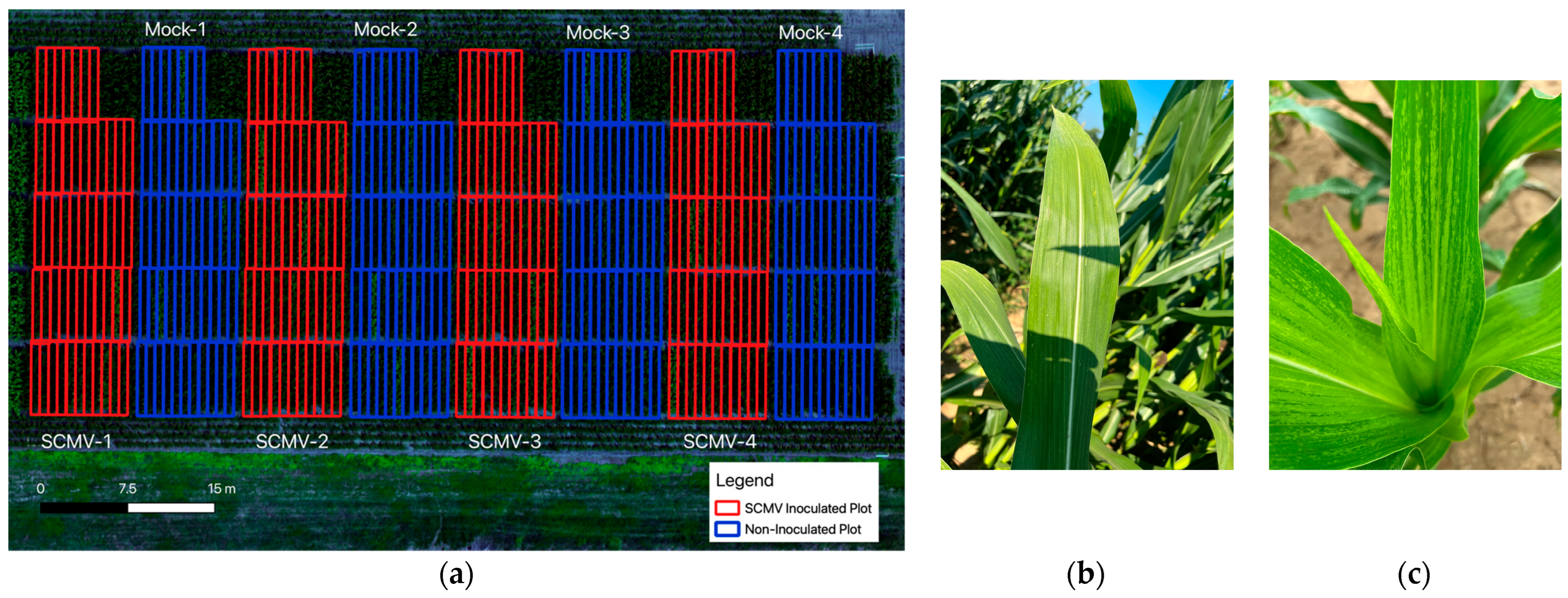
Figure 1. (a) Experimental layout in Synder field in 2021, overlaid on an aerial image captured on 14 July 2021. Red and blue boxes represent the randomized block design containing four single-row replicates of inoculated (red) and noninfected/mock-inoculated (blue) for each of the 51 hybrid varieties grown. (b) A corn crop that does not have SCMV infection or visual SCMV symptoms. (c) A corn crop that displays visual symptoms of SCMV infection.
Remotesensing 16 03296 g001
Figure 2. Experimental layout in Schaffter (a) and Synder (b) fields in 2022, overlaid on an aerial image captured on 1 September 2022, demonstrating randomized block designs with four 4-row replicates for each of the five hybrid varieties (including one control hybrid). Each box contains a unique plot number represented by a three-digit number, while the single-digit number corresponds to the hybrid group of that plot.
Remotesensing 16 03296 g002
Figure 3. Cumulative rainfall (mm), average daily air temperature (Celsius), and average daily relative humidity (%) for 2021 and 2022 corn field seasons (March–November). Rainfall is displayed as bar plots that accumulate value as season progresses. Data collected from Ohio State University CFAES Weather System at the Wooster Station.
Remotesensing 16 03296 g003
Figure 4. A flow diagram displaying the general methodological process implemented going from left to right. The best-performing regression models are identified for prediction of disease incidence percentage and binary classification prediction of disease presence. The best-performing models were further explored to identify the most important and most impactful features on the model’s performance. The number in parentheses for independent variables defines the number of variables included as a model input.
Remotesensing 16 03296 g004
Figure 5. Boxplots displaying (A) the disease incidence percentage values and (B) average yield values (bushels/acre), for each of the fields and years involved in the study for the SCMV-inoculated field plots. The solid black lines inside the plots represent medians, and the X marks represent the mean for each plot.
Remotesensing 16 03296 g005
Figure 8. Boxplots displaying the average values of the (a) simplified canopy chlorophyll content index (SCCCI) and (b) saturation index (SI) for SCMV-inoculated (red bars) and mock-inoculated (blue bars) samples across the growing season dates for both 2021 and 2022.
Remotesensing 16 03296 g008
Table 1. Summary of available data collected for each field by date.
Dates 1,2Snyder Field Schaffter Field
14 July 2021Multispectral, Thermal IRNA
28 July 2021MultispectralNA
28 July 2022 Multispectral, Thermal IR 3, LiDARMultispectral, LiDAR
1 September 2022Multispectral, Thermal IR 3Multispectral
1 Observations from plots (104, 204, 504, 604, 103, 203, 204, 604 in Figure 2b) across all dates in 2022 were excluded from the analyses due to flooding in the northwest corner of Snyder field. Additionally, observations from ‘hybrid 4’ were removed from analysis due to significant lodging. 2 All data collected during the June dates, i.e., 28 June 2021 and 30 June 2022, were excluded from machine learning model analyses as SCMV inoculation events had not yet been completed at this time, and, thus, the images do not reflect treatments implemented by the randomized block design. These portions of data were removed because any yield response or spectral response likely would not be due to the SCMV infection and would skew interpretation. The data from the June flights are only included in the model covered in Section 3.7, which includes data derived from additional sensors and also the models exploring the individual flight date performances. In total, 888 samples across both years were used for analysis across all flights and fields with 768 observations occurring in 2021 and 120 observations occurring in 2021. Additionally, in 2021, due to a data collection issue, multispectral imagery was only captured for 144 of the 408 sample plots on 28 June 2021. The in-house hybrid controls were also removed from model analysis. 3 Minor gaps were present in thermal orthomosaic representing 28 July 2022 and 1 September 2022 dates in Synder but were deemed useful to represent variations in canopy temperature due to SCMV inoculation. NA: not available.
Table 2. Vegetation indices (VIs) derived from the five-band multispectral images. VIs were used as features in modeling efforts.
Vegetation Index (VI)EquationReference
Brightness
Index (BI)
(((R2) + (G2) + (B2))/3)0.5[54]
Coloration Index (CI)(R − G)/(R + G)[54]
Chlorophyll Index Green (CIG)(NIR/G) − 1[55]
Chlorophyll Index Red-Edge (CIRE)(NIR/Rdg) − 1[55]
Chlorophyll Vegetation Index (CVI)NIR−(R/(G2))[56]
Enhanced Vegetation Index (EVI)(2.5 × (NIR−R))/((NIR + 6 × R−7.5 × B) + 1)[57]
Green Atmospherically Resistant Vegetation Index (GARVI)(NIR − (G − (B − R)))/(NIR + (G − (B − R)))[58]
Green Normalized Vegetation Index (GNDVI)(NIR − G)/(NIR + G)[59]
Green Wide Dynamic Vegetation Index (α = 0.1; gWDRVI 1)((0.1 × NIR − R)/(0.1 × NIR + R)) + ((1 − 0.1)/(1 + 0.1))[60]
Green Wide Dynamic Vegetation Index (α = 0.2, gWDRVI 2)((0.2 × NIR−R)/(0.2 × NIR + R)) + ((1 − 0.2)/(1 + 0.2))[60]
Hue Index (HI)(2 × R − G − B)/(G − B)[54]
Inverse Ratio Index (IRVI)R/NIR[61]
Neparian Logarithm of the Red-Edge (lnRE)100 × (lnNIR − lnR)[62]
Modified Chlorophyll Absorption Ratio Index 1 (MCARI 1)1.2 × (2.5 × (NIR − G) − 1.3 × (R − G))[63,64]
MCARI 2(3.75 × (NIR − R) − 1.95 × (NIR − G))/((((2 × NIR + 1)2) − (6 × NIR − 5 × sqrtI) − 0.5))[63,64]
Modified Chlorophyll Absorption Index/Optimized Soil-Adjusted Vegetation Index (MCARI/OSAVI)(((Rdg − R) − 0.2 × (Rdg − G)) × (Rdg/R))/(1.16 × ((NIR − R)/(NIR + R + 0.16)))[65]
Modified Soil-Adjusted Vegetation Index (MSAVI)(2 × NIR + 1 − sqrt(((2 × NIR + 1)2) − 8 × (NIR − R)))/2[66]
Modified Simple Ratio (MSR)((NIR/R) − 1)/(((NIR/R) + 1)0.5))[67]
Modified Triangular Vegetation Index 1 (MTVI 1)(1.2 × (1.2 × (NIR − G) − 2.5 × (R − G)))[64]
MTVI Index 2(1.8 × (NIR − G) − 3.75 × (R − G))/(sqrt(((2 × NIR + 1)2) − (6 × NIR − 5 × sI(R)) − 0.5))[64]
Normalized Difference Red-Edge (NDRE)(NIR − Rdg)/(NIR + Rdg)[68]
Normalized Difference Vegetation Index (NDVI)(NIR − R)/(NIR + R)[69]
Normalized Green/REd Difference Index (NGRDI)(G − R)/(G + R)[70]
Ratio between NIR and Green bands (NIR/G)NIR/G[59]
Ratio between NIR and Red bands or Ratio Vegetation Index (NIR/R) (or RVI)NIR/R[71]
Ratio between NIR and Red-Edge bands (NIR/R-Edge)NIR/Rdg[71]
Optimized Soil-Adjusted Vegetation Index (OSAVI)(1 + 0.16) × (NIR − R)/(NIR + R + 0.16)[65]
Renormalized Difference Vegetation Index (RDVI) (broadband)(NIR − R)/((NIR + R)0.5)[72]
Redness Index (RI)(R2)/(B × (G3))[54]
Soil-Adjusted Vegetation Index (L = 0.5, intermediate vegetation; SAVI)1.5 × ((NIR − R)/(NIR + R + 0.5))[73]
Simplified Canopy Chlorophyll Content Index (SCCCI)NDRE/NDVI or
N I R R d g / N I R + R d g N I R R / N I R + R
[68,74]
Saturation Index
or Normalized Pigment Chlorophyll Index (SI or NPCI)
(R − B)/(R + B)[54,75]
Transformed Chlorophyll Absorption Reflectance Index (TCARI) (broadband)(3 × ((Rdg − R) − 0.2 × (Rdg − G)) × (Rdg/R))[76]
TCARI/Optimized Soil-Adjusted Vegetation Index (TCARI/OSAVI)(3 × ((Rdg − R) − 0.2 × (Rdg − G)) × (Rdg/R))/(1.16 × ((NIR − R)/(NIR + R + 0.16)))[76]
Wide Dynamic Vegetation Index 1 (α = 0.1; WDRVI 1)(0.1 × NIR − R)/(0.1 × NIR + R)[60]
WDRVI Index 2 (α = 0.2; WDRVI 2)(0.2 × NIR − R)/(0.2 × NIR + R)[60]
Note: The center wavelength and bandwidth of the five spectral bands included B—blue band (475 nm, 32 nm), G—green band (560 nm, 27 nm), R—red band (668 nm, 16 nm), Rdg—red-edge (717 nm, 12 nm), and NIR—near-infrared (842 nm, 57 nm).
Table 3. Top vegetative indices and spectral bands with statistically significant correlation with disease incidence at each trial location.
2021Snyder Farm2022Snyder FarmSchaffter Farm
14 July 2021SCCCI = −0.4028 July 2022Not SignificantNGRDI = 0.61
TCARI/OSAVI = 0.3
MACARI/OSAVI = 0.3CI = −0.61
CVI = 0.26HI = −0.60
28 July 2021SCCCI = −0.311 September 2022NIR = −0.63MCARI2 = 0.56
NDRE = −0.24
CIRE = −0.24MCARI1 = −0.61NIR/Red = 0.56
NIR/Red = −0.24MTVI1 = −0.56MSR = 0.56
Table 4. Model performances for prediction of disease incidence percentage by year.
Models202120222021 and 2022 Combined
R2RMSER2RMSER2RMSE
Ridge Regression0.3028.780.0239.500.2130.99
Support Vector Regression0.3926.52−0.0639.340.2530.43
Random Forest0.4026.23−0.1140.280.2929.35
XGBoost0.4026.32−0.0739.660.2929.26
Note: Models used 41 features as independent variables, and R2 and RMSE are the average of three model repetitions using three unique ‘seeds’ for partitioning training and testing data.
Table 5. Performance of XGBoost model for prediction of disease incidence percentage by flight date.
DatesR2RMSE
28 June 20210.0333.98
14 July 20210.3528.14
28 July 20210.4326.19
30 June 2022−0.3241.94
28 July 2022−0.2038.85
1 September 2022−0.1037.16
Note: Models used 41 features as independent variables, and R2 and RMSE are the average of three model repetitions using three unique ‘seeds’ for partitioning training and testing data.
Table 6. Accuracy of classification models for predicting SCMV-inoculated vs. mock-inoculated plots.
Models202120222021 & 2022
Support Vector Machine0.7590.3610.729
Random Forest0.7420.4720.708
XGBoost0.7560.4170.705
Note: Models included 41 spectral features. Accuracy reported is the average of three model runs with three unique ‘seeds’ for partitioning training and testing data.
Disclaimer/Publisher’s Note: The statements, opinions and data contained in all publications are solely those of the individual author(s) and contributor(s) and not of MDPI and/or the editor(s). MDPI and/or the editor(s) disclaim responsibility for any injury to people or property resulting from any ideas, methods, instructions or products referred to in the content.