Abstract
When assessing radar anti-jamming performance, the challenge of limited sample sizes is a significant hurdle. In response, this paper introduces a logistic fusion model that leverages Bayesian techniques and a Monte Carlo Markov chain (MCMC) sampling method based on a logistic regression model that characterizes the relationship between the signal-to-interference ratio (SIR) and the anti-jamming rate. The logistic curve’s inflection point and growth rate serve as crucial indices for evaluating radar anti-jamming performance, providing insights into the SIR threshold for successful jamming mitigation. The proposed model allows for the derivation of posterior distributions for these parameters using the MCMC sampling method and kernel density estimation. It also enables the fusion of anti-jamming data from multiple stages, including mathematical simulations, hardware-in-the-loop tests, and field tests. Through extensive simulations, our method achieves a remarkably low root mean square error (RMSE) of . Compared with a conventional BETA fusion model, our proposed logistic fusion approach demonstrates superior performance and robustness in accurately estimating the anti-jamming rate. The fusion of multi-stage data, even with varying levels of reliability, improves the overall accuracy of the performance evaluation.
1. Introduction
The contemporary electromagnetic environment surrounding radar systems has grown increasingly intricate, emphasizing the critical need for accurate and consistent evaluation results for effectively gauging countermeasure scenarios [1,2]. Evaluating a radar’s anti-jamming capability within jamming environments holds significant practical value in the realm of electronic countermeasures [3].
Traditionally, radar anti-jamming performance evaluation has focused on constructing evaluation index systems and assigning weights. Methodologies such as the analytic hierarchy process (AHP) [4,5], the Technique for Order Preference by Similarity to Ideal Solution (TOPSIS) [6], D-S evidence theory [4,7], and expert scoring are commonly utilized, with subsequent layer-by-layer integration of evaluations. However, these methods are limited by their inherent subjectivity. To enhance objectivity, researchers have incorporated techniques like support vector machines (SVMs) [8] and the entropy weight method (EWM) [9]. Despite these advancements, the effectiveness of these methods remains heavily dependent on the quality and availability of underlying data, making them less effective in scenarios with limited or unreliable samples.
In response to these questions, data fusion has emerged as a critical tool. Existing data fusion methods across the fields of image fusion [10,11,12,13], sensor fusion [14,15], and signal-level fusion [16,17] have been explored for evaluating fusion effectiveness. However, these methods often fall short in scenarios involving multi-stage data fusion, particularly in scenarios where sample data are scarce.
Evaluating a radar’s anti-jamming capability is challenging with limited samples. This is often due to high costs or complex testing procedures. In such cases, it becomes necessary to fuse data from various sources and stages, which presents two main challenges. First, ensuring coherence across diverse information sources is vital for establishing a solid foundation for information fusion. Second, determining the appropriate weights for the information is a crucial consideration.
To tackle the first challenge, various data fusion algorithms and models have been developed. For example, the K-L information distance measurement method verifies data consistency for fusion purposes [18]. Regarding the second challenge, studies have integrated the confidence factor into data fusion algorithms, adaptively reducing the fusion weight of erroneous data and mitigating adverse factors in the detection process [19]. Moreover, an adaptively weighted fusion method has been applied to fuse multi-sensor data [20]. When considering data fusion across different stages, a Markov chain model has been suggested to evaluate radar anti-jamming capabilities. It incorporates data from the anti-jamming search–detection–tracking process through transition probability [21].
Traditional fusion methods may not adequately account for the distinct characteristics, reliability, and sample sizes of data from different stages such as mathematical simulations (MS), hardware-in-the-loop (HWIL) tests, and field tests (FT), highlighting the need for a more robust approach. In our previous work [22], we introduced a signal-to-interference ratio fusion (SIRF) model that integrated multi-stage data by considering radar cross-section (RCS) fluctuation models and radar target distances. This model, grounded in Bayesian theory and anti-entropy weight methods, is particularly effective in scenarios requiring detailed RCS and target distance information. However, in this paper, we propose a more versatile approach that can adapt to scenarios where such detailed information may not be available.
While traditional fusion methods often focus solely on deriving average anti-jamming results, scenarios might occur where both large and small datasets produce identical regression outputs, which could overlook important nuances in the data and potentially lead to inaccurate assessments of anti-jamming performance. In practice, datasets of varying sizes carry distinct levels of credibility, a subtlety that traditional frequentist fusion methods struggle to capture effectively.
To address these limitations, this paper introduces a novel logistic fusion model that transcends specific radar types. By focusing on SIR data and corresponding anti-jamming results, our model employs a Bayesian fusion method to integrate data from different stages, test environments, and systematic errors. This approach uses Monte Carlo Markov chain (MCMC) sampling and kernel density estimation to derive posterior distributions for key parameters, allowing for dynamic data fusion that accommodates different sample sizes and levels of systematic error across stages. We demonstrate that this model provides more reliable evaluation results, particularly in scenarios where real-world data are sparse or of varying quality across testing stages.
The structure of this paper is organized as follows. Section 2 introduces the logistic fusion model, detailing the mathematical foundation and the MCMC sampling process used to estimate the model’s parameters. Section 3 presents two examples of the model’s application, showcasing the fusion of three-stage data and comparing the results with those obtained from other methods. The conclusion summarizes the key findings along with providing suggestions for future research directions.
2. Logistic Fusion Model and the MCMC Fusion Method
In this section, we introduce the logistic fusion model and the MCMC sampling method: both are crucial for estimating radar anti-jamming performance.
The logistic fusion model characterizes the relationship between SIR values and the success or failure of anti-jamming efforts. It serves as a key index for evaluating radar anti-jamming capabilities, providing insights into the SIR thresholds necessary for effective jamming mitigation. The MCMC sampling process is used to estimate the posterior distribution of the model’s parameters.
This section is dedicated to the conceptual framework, methods, and tools essential for our approach.
2.1. Definition of the Logistic Fusion Model
Our proposed method is primarily designed to evaluate radar anti-jamming performance against noise jamming based on different SIR levels. We begin by revisiting the concept of the SIR and its significance in relation to anti-jamming outcomes. The SIR, typically denoted as , serves as a critical metric for evaluating the performance of radar systems in the presence of jamming. It is defined as the ratio of target echo power () to jamming power (), as expressed in Equation (1). This metric directly determines the anti-jamming result and reflects the radar’s anti-jamming effectiveness in scenarios with interfering jamming signals [18].
When the SIR is sufficiently high, the radar can detect the target amidst jamming interference, indicating successful anti-jamming. Conversely, when the SIR is low, the radar fails to detect the target, resulting in unsuccessful anti-jamming. In practical scenarios, the data available to us typically consist of binary outcomes, success or failure, corresponding to the radar’s anti-jamming performance. This binary classification problem is central to our analysis. We denote by y the anti-jamming result, which takes the value 1 or 0, representing success or failure of radar anti-jamming, respectively. In this context, the data we can obtain and use are represented as pairs of (SIR, y).
The logistic regression model is fundamentally designed to handle binary outcomes. In our case, the radar anti-jamming performance can be seen as a binary classification problem for which the outcome is whether the radar system successfully resists jamming (anti-jamming rate). In fact, using logistic functions to model radar anti-jamming performance is a common practice [23,24,25,26]. Here, we also posit that the relationship between the SIR and the anti-jamming rate can be effectively captured by a logistic model, as depicted in Equation (2).
where x represents the SIR, signifies the radar anti-jamming rate, and and are the model parameters. The logistic function, as given by Equation (2), naturally models an S-shaped curve, which is suitable for scenarios where the probability of success increases with the SIR in a non-linear fashion.
The inflection point, , and the growth rate, , are crucial parameters for evaluating radar anti-jamming performance. When the SIR exceeds the inflection point, the anti-jamming rate rapidly approaches 1, indicating successful jamming mitigation. Conversely, lower SIR values result in anti-jamming rates approaching 0, signifying failure. The growth rate determines the transition rate from 0 to 1 anti-jamming probability.
Given that anti-jamming outcomes are binary (success or failure, represented by 1 or 0), we use Bernoulli random variables to describe the anti-jamming test events corresponding to each SIR, represented by x. For each SIR, the mean of is assumed to be , so follows
The anti-jamming data comprise pairs of SIR data and anti-jamming results. They are denoted by , where represents SIR samples and represents samples of corresponding binary anti-jamming results. Here, and represent the prior distributions of and , respectively. In the model framework, we make the assumption that and are independent random variables [27,28]. Hence, . is the likelihood function, and represents the posterior parameter distributions based on the observed data X.
We consider the logistic fusion model as in Equations (2) and (3) and use the formula for Bayes’ theorem. The scaled posterior distribution of and can be expressed as
This setup lays the groundwork for our subsequent analysis of radar anti-jamming performance, which uses the logistic fusion model and MCMC sampling method. Note that our fusion evaluation model not only combines data with varying SIR levels but also fuses data from different testing stages. These all contribute to the reliability and accuracy of radar anti-jamming performance evaluation.
2.2. MCMC Sampling Process
MCMC is a powerful stochastic simulation technique rooted in Markov chain theory. It is employed for sampling from complex probability distributions. Fundamentally, MCMC generates samples that conform to a target probability distribution by constructing a Markov chain with a stationary distribution equivalent to the target distribution. The method accomplishes this by simulating the evolution of the Markov chain, where each step represents a transition from one state to another. Various MCMC algorithms have been developed to facilitate this sampling process, including well-known methods such as Metropolis–Hastings, Gibbs, Slice, and other sampling techniques [29].
Slice sampling is an MCMC algorithm that is specifically designed to efficiently sample from probability distributions, particularly in scenarios where traditional methods may be impractical or challenging to implement. Introduced by Neal in [30], slice sampling offers a simple approach that eliminates the need to specify proposal distributions. This makes it particularly appealing for complex and high-dimensional distributions. MCMC parameter estimation involves considering prior distributions, likelihood functions, and posterior distribution. By iteratively sampling from the scaled posterior distribution using slice sampling algorithms, we may infer the model parameters and their uncertainties.
After obtaining the scaled posterior distribution of and , the next step is utilizing the slice sampling method to generate samples from this distribution to approximate the posterior distribution of the parameters. We start by selecting an initial point in the parameter space. We then conduct slice sampling iterations, which involves the following steps:
- Sample slice variable: Choose a value z uniformly from the interval .
- Update parameters: Update by sampling a new point from the slice defined by . This involves iteratively sampling along the slice until a suitable point is found.
- Repeat: Repeat the above steps for a sufficient number of iterations to obtain a representative sample from the posterior distribution .
To illustrate the MCMC sampling process, let us consider an example. We assume Gaussian prior distributions for both parameters and generate stage data X based on Equations (2) and (3) with and .
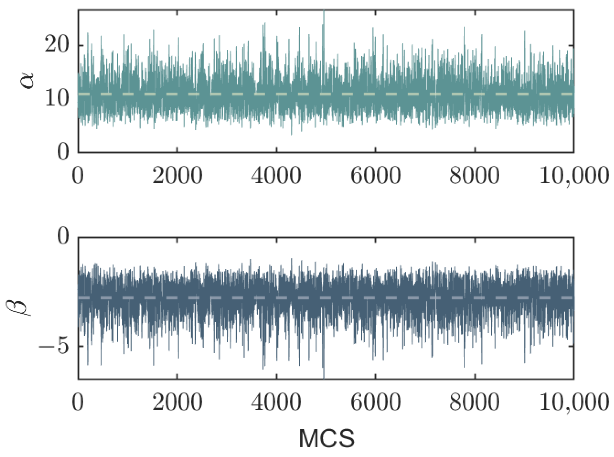
We exclude a burn-in phase of 2000 samples and observe the Markov chains attaining stationarity, as depicted in Figure 1, where the chains exhibit fluctuations around their means. We set the maximum iteration steps to 100,000 and collect samples at intervals of 10 steps, yielding a total of 10,000 Monte Carlo steps (MCS; 1 MCS = 10 iteration steps) for estimating the posterior parameter distribution.
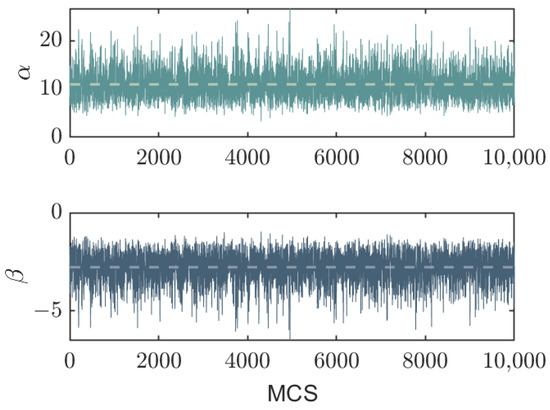
Figure 1.
Traces of and in a typical MCMC sampling process with a burn-in phase of 200 MCS (1 MCS = 10 iteration steps). We consider prior distributions for both parameters following a Gaussian distribution , while the stage data X are generated based on Equations (2) and (3) with specific values of and . The horizontal dashed lines represent the sample means for the respective parameters.
Subsequently, we utilize these samples to construct histograms, exemplified in Figure 2, displaying single-peaked distributions shaped by both the prior distribution and the observed data X.
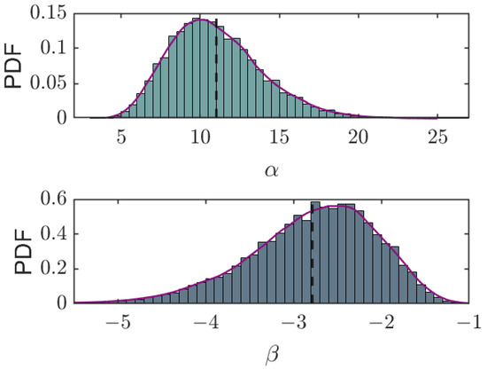
Figure 2.
Posterior distribution histograms of and from their respective traces, as shown in Figure 1. The vertical dashed lines represent the sample means for the respective parameters, and the purple fitting curves are obtained by the kernel density estimation.
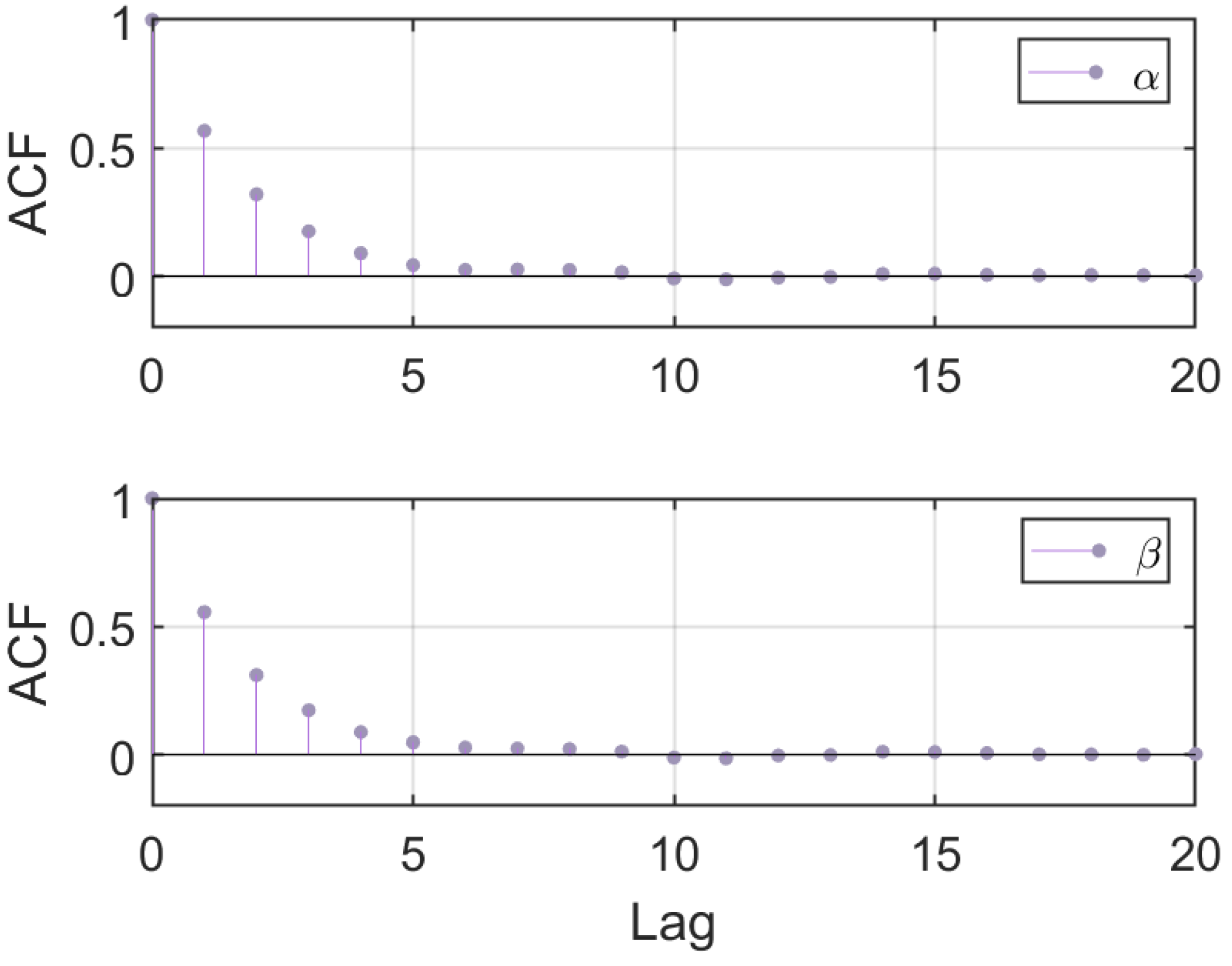
To assess the convergence of the Markov chains, we employ the autocorrelation function (ACF) to evaluate the correlation among the samples (see Figure 3). The ACF graphically represents the correlation coefficients between the parameter sampling sequence and its lagged samples on a bar graph. The x-axis denotes the lag number and the y-axis denotes the autocorrelation coefficients.
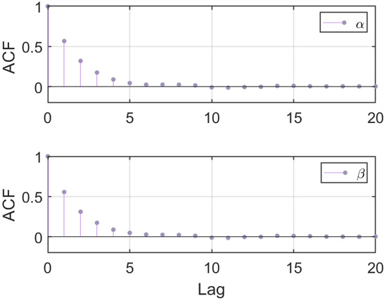
Figure 3.
Autocorrelation function of and . The rapid decrease in autocorrelation towards 0 suggests that the Markov chain is converging to its stationary distribution and producing independent samples.
The relatively high autocorrelation coefficient for small lag numbers indicates strong correlation between the current parameter sampling values and their immediate past values. It suggests that the Markov chain is exploring the parameter space and potentially moving in a correlated manner. Then, the rapid decrease in autocorrelation towards 0 suggests that the Markov chain is converging to its stationary distribution and producing independent samples. This behavior indicates that the MCMC method has reached a stable state and that the parameter estimates are reliable and representative of the posterior distribution.
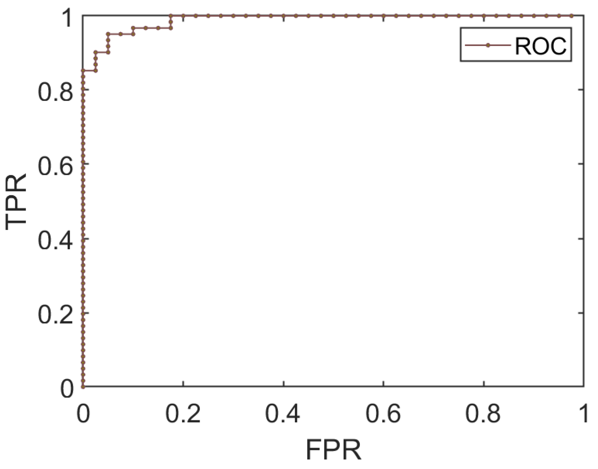
The goodness of the MCMC method for predicting the logistic curve parameters, which reveals the relationship between the SIR and anti-jamming results, can be evaluated using the receiver operating characteristic (ROC) curve. The ROC curve is a graphical representation of the trade-off between the true positive rate (TPR or sensitivity) and the false positive rate (FPR) at various classification thresholds. The TPR is the proportion of positive samples correctly identified by the model, while the FPR is the proportion of negative samples incorrectly classified as positive.
As shown in Figure 4, the ROC curve demonstrates that the MCMC method’s results align well with the real observations. The area under the ROC curve (AUC) quantifies the overall performance of the model, with higher values indicating better predictive ability. In this study, the AUC value of suggests an excellent fit between the model’s predictions and the true anti-jamming rates.
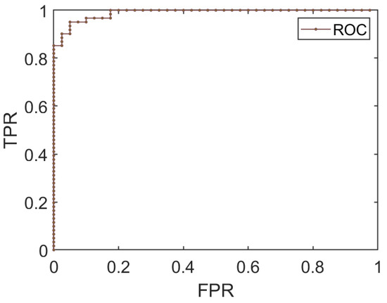
Figure 4.
ROC curve depicting the performance of the logistic model for binary classification. The ROC curve is close to the upper left corner, indicating a higher TPR and a lower FPR, which suggests a strong fit of the logistic model to the data. Parameters of the logistic curve are derived from mean values of the posterior distributions obtained through MCMC sampling.
2.3. Multi-Stage Bayesian Fusion Process
In the context of the multi-stage fusion process for evaluating radar anti-jamming performance using the logistic fusion model, the goal is to obtain accurate estimates of the parameters and . However, systematic errors may vary across the stages—MS, HWIL, and FT—affecting the expected values of these parameters. These errors can be quantified through distinct deviations for and at each stage. Thus, the logistic model at each stage can be expressed as:
Here, denotes the anti-jamming rate obtained from stage j (where correspond to the MS, HWIL, and FT stages, respectively). The terms and represent the magnitudes of the systematic errors associated with the parameters and at stage j.
The MS stage typically provides abundant samples but exhibits the largest systematic error. In contrast, the HWIL stage offers a moderate sample size with a moderate systematic error, while the FT stage has the smallest systematic error but limited sample availability. Despite the higher systematic error in the MS stage, the abundance of samples enhances the robustness of fusion results. Relying solely on FT stage data could lead to less stable parameter estimations due to the scarcity of samples.
To optimize the fusion process, it is advantageous to combine data from all stages—MS, HWIL, and FT—leveraging the strengths of each. Denoting the data samples from the stages as ( corresponding to the MS, HWIL, and FT stages, respectively) and the corresponding sample sizes as , a Bayesian approach is employed.
We posit that and are two independent random variables. When the samples from the MS stage are incorporated, then
Here and in the following, we assume the prior and follow a Gaussian distribution, and the likelihood function is determined by the logistic fusion model as in Equations (3) and (5). The form of it can be referred to as in Equation (4).
The MCMC sampling process begins with setting initial parameter values . Then, the posterior distribution of the parameters is calculated by incorporating stage sample data, leading to the generation of parameter traces. The traces are then used to construct the posterior distribution histograms of .
Then, a kernel density estimation technique with the Epanechnikov kernel [31] is employed to fit the posterior distribution. This fitted posterior distribution, denoted as , serves as the prior distribution for the subsequent stage.
The Epanechnikov kernel function, which is a quadratic function, is more efficient due to its polynomial nature and bounded support. In contrast, the Gaussian kernel function is more computationally expensive. Moreover, the Epanechnikov kernel function is optimal for minimizing the mean square error, enhancing the accuracy of the density estimation process [31].
We have conducted a brief comparison of the computation efficiency and root mean square error (RMSE), which measures the average difference between a statistical model’s predicted values and the actual values [22], between two kernels: namely, KernelE representing the Epanechnikov kernel and KernelG representing the Gaussian kernel. Table 1 presents the results, which are obtained by running 100 experimental instances and averaging the execution time and RMSE. The execution time is evaluated based on the following computer configuration: CPU: Intel (R) Core(TM) i7-10875H CPU@2.30 GHz, 2304 MHz; RAM: 16 GB; and operating system: Windows 11. The results show that the Epanechnikov kernel function consistently outperforms the Gaussian kernel function in terms of execution time, especially for large datasets. Additionally, we compared the RMSEs of the estimations, which demonstrates that the Epanechnikov kernel achieves a lower RMSE in our scenarios. It is important to note that radar systems typically employ onboard computer platforms or embedded systems for real-time processing. The results presented here serve as a preliminary evaluation, and further testing on an embedded system is necessary to fully assess the real-time applicability of the proposed anti-jamming algorithm.

Table 1.
Comparison of algorithm efficiency for different kernel estimations.
The iterative process involves updating the posterior distribution at each stage by combining the likelihood function with the prior distribution obtained from the preceding stage.
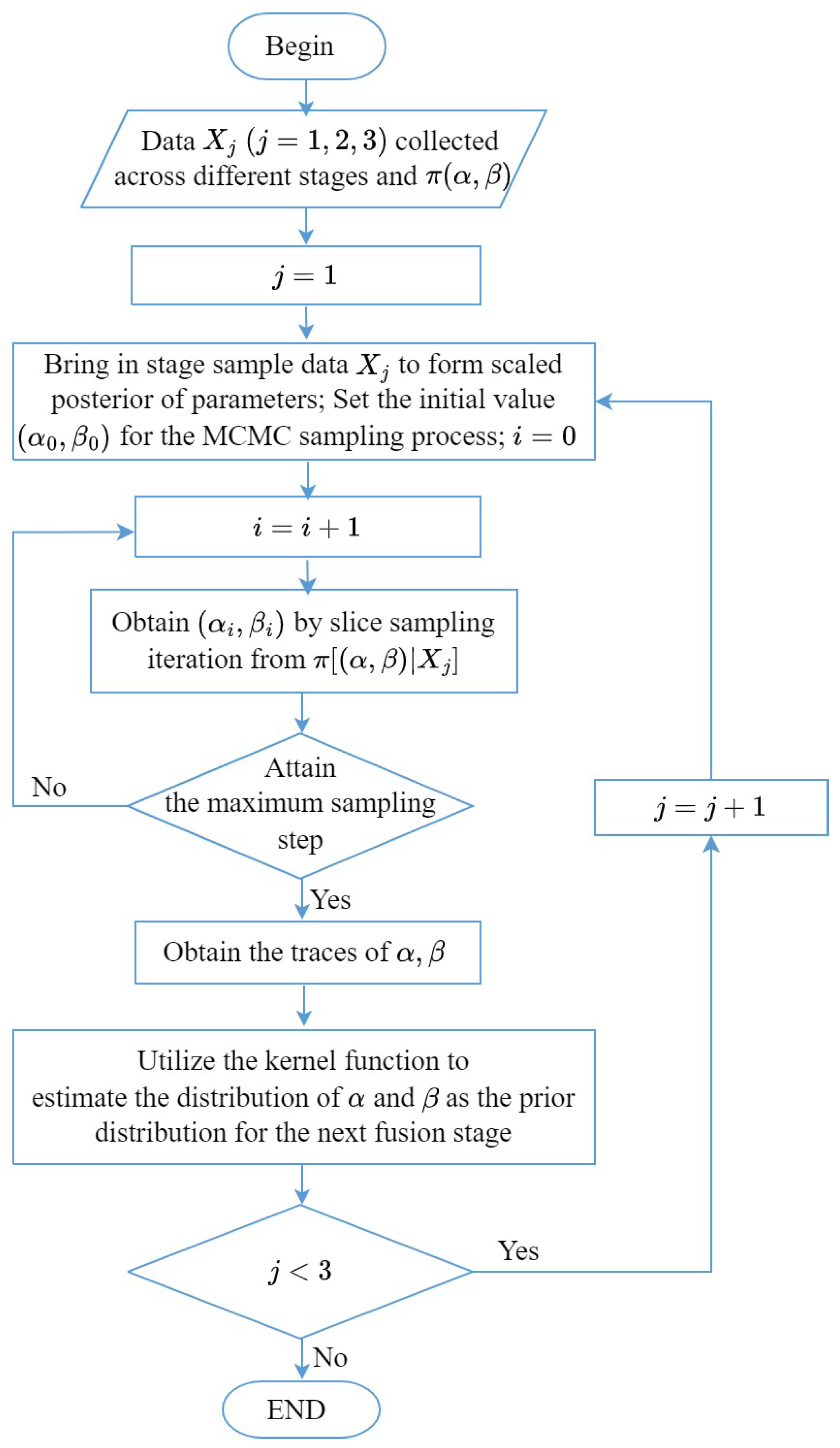
This iterative Bayesian fusion process continues until all stage data are fused. A brief illustration of the whole Bayesian fusion procedure is shown in Figure 5.

Figure 5.
Illustration of the multi-stage Bayesian fusion process incorporating MCMC sampling and kernel density estimation. Stage sample data consist of pairs of SIR and anti-jamming results across different stages. The prior distributions for the parameters within the logistic fusion model and the stage sample data are used to formulate the scaled posterior distribution. Subsequently, the MCMC sampling process is executed to generate parameter traces. These traces are then utilized in a kernel density estimation procedure to fit the posterior distribution. The resulting fitted posterior distribution acts as the prior distribution for the subsequent stage, creating an iterative process. This iterative loop iterates through the stages until the fusion of data from all sample stages is successfully completed.
Assessing radar anti-jamming rates across varying SIR levels is a critical performance metric. The mean values of the parameters obtained from their distributions at each stage can be incorporated into the logistic fusion model to derive the radar anti-jamming rate curves. Traditional radar anti-jamming evaluation methods, particularly those grounded in the frequentist perspective, often produce a single fusion result, lacking the ability to offer a comprehensive distribution of outcomes.
One of the key advantages of Bayesian fusion is its capability to provide distributions of the fused parameters. The distributions provide valuable insights into the uncertainty associated with the parameters and allows for a comprehensive understanding of the model’s behavior. By leveraging these distributions, we can establish the probability distribution of radar anti-jamming rates across varying SIR levels.
Obtaining both the mean anti-jamming rate and its distribution across different SIR levels enables a more nuanced understanding of the system’s performance. This capability becomes particularly valuable when dealing with scenarios involving limited data samples.
3. Fusion Results
This section focuses on the practical application of our proposed method, using two examples that involve the fusion of three-stage data.
We start by outlining the data generation scheme. In real-world scenarios, data from the MS, HWIL, and FT stages would typically be derived from physical testing of radar systems. However, conducting these tests requires significant resources, time, and controlled conditions, which may not always be feasible for every study. To effectively demonstrate our method while maintaining flexibility and control over the experimental parameters, we generate synthetic data that reflect the distinct characteristics of these three stages.
We then present two fusion examples using this synthetic data, followed by a comparison of our results with those obtained from alternative methods. Finally, we discuss the limitations of our model.
3.1. Data Generation Scheme
In real scenarios, MS, HWIL, and FT sample data would typically come from actual physical testing of the radar system. For instance, suppose the parameters of an airborne self-defense jammer and a terminal guidance radar are as follows: radar transmit power kW, antenna gain dB, radar cross-section , radar target distance km, jammer power kW, jammer antenna gain dB, and bandwidth MHz. The MS data may involve initial modeling and simulation studies, while HWIL testing would be conducted using hardware components in a controlled laboratory environment. Finally, FT data would be collected during field trials or operational deployments of the radar system in real-world conditions.
As said in the last section, the data characteristics across these stages exhibit distinct sample sizes and levels of systematic errors. The MS stage typically has the largest sample size and highest systematic error. The HWIL stage has a moderate sample size and systematic error. The FT stage has the smallest sample size and systematic error. To assess the efficacy of the fusion model, synthetic data are generated to mirror these characteristics rather than utilizing sensitive and costly real-world data.
The focus is on data with SIR values in the range of . Different sample sizes are generated for each stage, with the MS stage having the highest sample density, followed by the HWIL stage, and with the FT stage having the lowest sample density. This reflects the abundance of samples in the MS stage, a moderate sample size in the HWIL stage, and scarcity in the FT stage.
Moreover, it is assumed that each stage exhibits distinct systematic errors. For the FT stage, environmental variations such as temperature, pressure, and humidity can be the source of errors. For the HWIL stage, imperfections in actual hardware components, synchronization issues between hardware and software, and latency in data transfer can be the source of errors. For the MS stage, inaccuracies in the models, including incorrect assumptions about the environment or simplifications of physical phenomena, can be the source of the errors. These systematic errors can manifest in various ways, such as constant offsets or scaling factors. The nature of these errors is often dependent on the specific equipment, conditions, and interactions of components within the simulation or test environment. It is important to note that the specific form of systematic errors is not crucial here. Instead, what matters are the final deviations of the parameters, denoted by and , which cause systematic deviations in the samples across different stages, i.e., MS, HWIL, and FT. These deviations, in turn, influence the final fusion results.
As for the following example, we preset the values of and ; then, by Equation (5), the anti-jamming rate curve against the SIR for each stage is determined. The SIR levels, selected for each stage as outlined previously, are then used to generate corresponding samples. For each SIR, from the anti-jamming rate curve, the corresponding anti-jamming rates is directly obtained by Equation (5), which signifies the likelihood of achieving success (1) or failure (0) in the anti-jamming process. The anti-jamming outcome (or result) is assumed to follow a Bernoulli distribution for each SIR level, with the mean equal to the anti-jamming rate.
3.2. Fusion Examples
To illustrate the effectiveness of our proposed logistic fusion model, we present two typical fusion examples. We set the actual values of and as and , with for the FT stage. This consideration reflects our regard for the FT stage data as the most accurate, although it may still carry errors. In the following examples, we assume the first one does not carry systematic errors for the growth rates () of the logistic curves across different stages, while the second example carries systematic errors for both the growth rates and the inflection points.
Example 1: For the first example, set . The terms and for the MS and HWIL stages. This caters to the case where the systematic errors of the growth rates for the logistic curves across the three stages can be ignored since for . However, the locations of the inflection points () of the logistic curves have different errors across different stages. Due to the existence of systematic errors, the inflection points across the three stages can be calculated as , respectively.
Example 2: For the second example, set , , and . In this case, the systematic errors for both the growth rates and inflection points cannot be ignored across different stages. The inflection points across the three stages can be calculated as approximately , respectively, while the growth rates can be calculated as , respectively.
All of these settings reflect the varying levels of accuracy across the different stages. Following the data generation scheme described earlier and with the preset system errors, we generate three samples for each SIR value across different stages, with SIR values incrementing at varying intervals:
- —
- For the MS stage, samples are generated with SIR increments of within the interval , reflecting the abundance of samples in this stage.
- —
- For the HWIL stage, samples are generated with SIR increments of within the interval , representing a moderate sample size.
- —
- For the FT stage, samples are generated with SIR increments of 1 within the interval , reflecting the scarcity of samples in this stage.
We then conduct a multi-stage Bayesian fusion procedure. Initially, using the MS stage samples and assuming Gaussian prior distributions for both parameters, we employ the MCMC method to obtain the posterior distributions of and via Equation (4). These posterior distributions, denoted as , serve as the prior distributions for the subsequent HWIL stage fusion via Equation (7). Finally, we fuse the FT stage data in a similar manner.
The MCMC method provides us with the joint probability density of the pair . For the two examples, we present color plots of the joint posterior density in Figure 6. At the MS stage, the distribution of is generally broad, indicating a wide confidence interval. As we move to the HWIL and FT stages, the distribution becomes narrower, suggesting more concentrated prediction results as we fuse more data. Comparing the two examples, the former has a consistent growth rate of across all stages, leading to more concentrated prediction results for . While for the second example, due to the existence of systematic errors, the growth rates are set to be , respectively. Although the preset value of , which equals , is slightly different from the predicted mean of , shown in Figure 6d, we consider this a reasonable prediction given the systematic errors in the MS and HWIL stages.
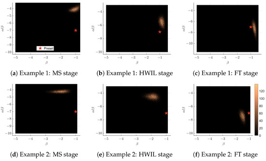
Figure 6.
Color plots of the joint posterior density estimations of the logistic parameters (growth rate) and (inflection point) after fusing samples from different stages for two typical examples. The color plots depict the joint probability density, with brighter regions indicating higher density values. The density estimation is based on 10,000 MCMC samples, with color intensity representing the number of samples in each bin. As more reliable samples are incorporated, especially from the FT stage, the posterior distributions converge closer to the true parameter values (marked by the red stars), indicating improved estimation accuracy.
In contrast, the posterior density of becomes wider as we progress from the MS to the HWIL to the FT stage for the two examples, indicating that the uncertainty of increases as more data are incorporated and fused. We presume that this is because data from different stages are generated with different inflection points for the logistic model (2). The ratio is more sensitive to data generated with different parameters, as fluctuations in both and contribute to the fluctuation of .
The preset value of , which equals 7 for both examples, falls into the confidence interval of the fusion prediction results, as shown in Figure 7. The histograms peak about their means, which are approximately and , respectively. As mentioned earlier, the distribution of is broader than those obtained from the previous two stages, reflecting the discrepancy of data samples generated from the logistic model with different inflection points. Specifically, the distribution for the former is much broader, which reflects the fact that the systematic deviation of the inflection point for the HWIL stage is larger (6, compared to for the latter). This further demonstrates that the fusion posterior distribution of is more sensitive to data generated with different parameters.
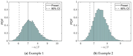
Figure 7.
Histogram illustrating the probability density of the fused parameter representing the inflection point of the logistic curve following data fusion from all the stages. The dotted line indicates the preset value of the inflection point , and the dashed lines give the boundaries of the 90% confidence interval for this parameter.
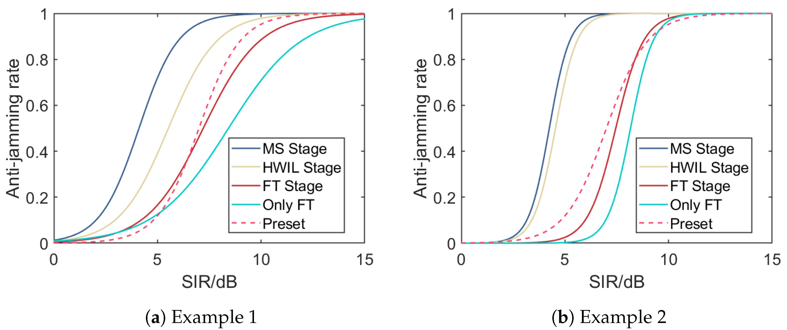
Using the mean parameter values obtained from the fusion results at each stage, we plot the predicted logistic curves in Figure 8. It can be observed that as more reliable samples are incorporated from the MS, HWIL, and FT stages, the fused logistic curve progressively converges towards the preset true curve. It is notable that our final fusion result surpasses the curve fitted solely using the FT stage data. This indicates that even though the MS and HWIL stages carry systematic errors, fusing data from these stages promotes the overall robustness and reliability of parameter estimations, especially when there are few samples for the FT stage.
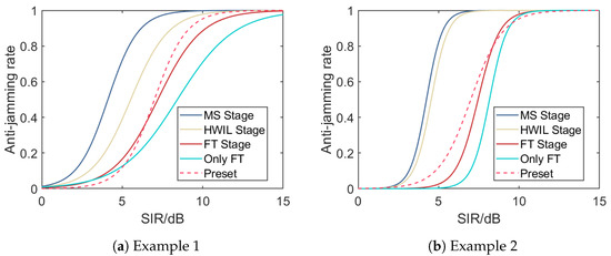
Figure 8.
Logistic curves illustrating the relationship between the anti-jamming rate and SIR using parameters obtained from each fusion stage for the two typical examples. As samples of increasing confidence are progressively fused from the MS to the HWIL and FT stages, the curves converge towards the one generated using preset parameters. The logistic fusion model yields a curve that aligns more closely with the preset value than a curve fitted exclusively from the limited FT stage samples, highlighting the benefit of our approach. Despite systematic errors in data samples from different stages, our Bayesian fusion process enhances the reliability and robustness of the final results, demonstrating that even less reliable data contribute to parameter predictions.
Comparing the fusion results for the first example (Figure 8a) with those for the second example (Figure 8b), the former has less variation in growth rates across fusion stages, where we assume that the parameter has a consistent value of . In contrast, for the latter, has different values due to systematic errors across the three stages; these values are , respectively.
We stress again that although the FT stage samples are the most reliable and closest to the true values, their limited quantity can lead to fluctuations and instability in the parameter fitting process. By incorporating samples from the MS and HWIL stages, despite their lower individual reliabilities, their collective contribution enhances the explanation of the underlying phenomenon. Therefore, fusing multi-stage data, even with those less reliable data, proves necessary and effective for accurate estimation of radar anti-jamming performance.
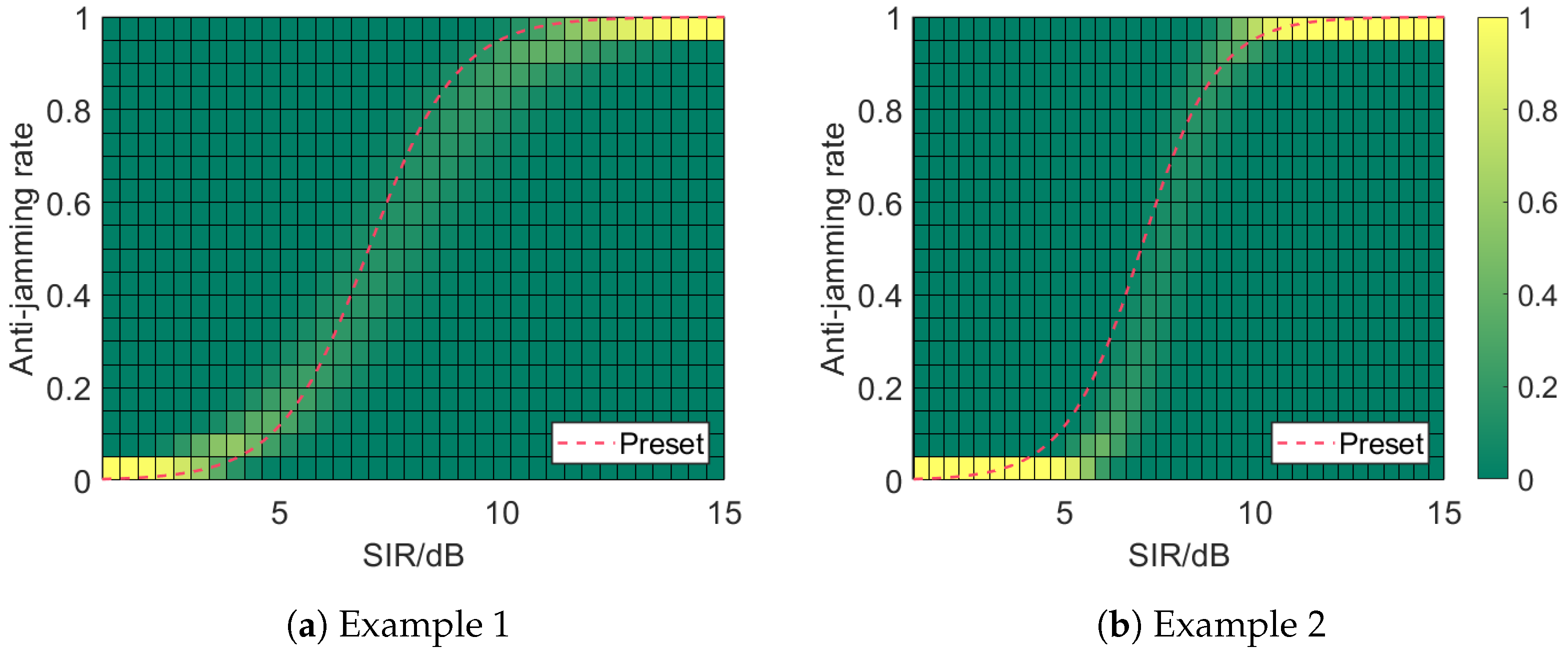
After obtaining the posterior distributions of the logistic fusion model parameters, we can derive the probability density of the anti-jamming rate, as shown in Figure 9. The regions of higher probability density for each SIR level trace a curve aligned with the preset true performance, which is shown as the dashed line. The slight discrepancy in the SIR around the transition regions is directly due to the discrepancy in our prediction of and , as discussed earlier and which we consider inevitable.
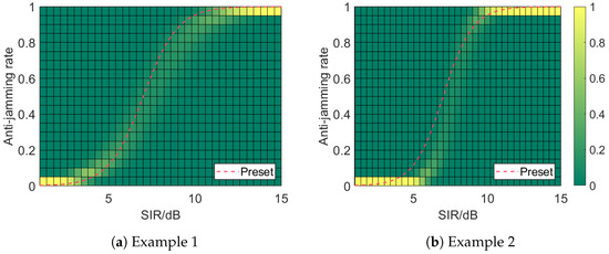
Figure 9.
Color plots of the probability densities of the anti-jamming rates after fusing samples from the FT stage. Brighter colors indicate regions of higher probability. The regions of higher probability for each SIR level trace a curve aligned with the preset parameters, reflecting the actual radar system performance. Note that our logistic fusion model yields a probability distribution rather than a single value for the anti-jamming rate.
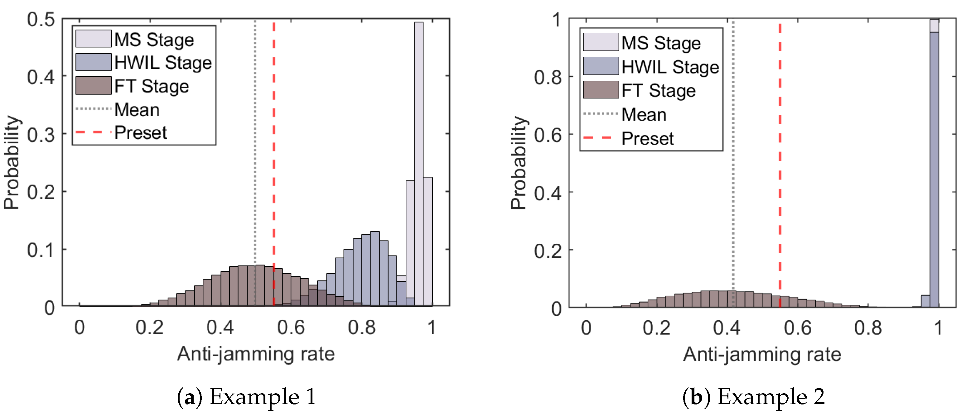
Figure 10 illustrates the predicted probability distributions (histograms) of the anti-jamming rates after fusing samples from each stage for a specific SIR value of . Due to the presence of systematic errors, the fusion model at the MS and HWIL stages yields overconfident probability distributions concentrated near 1 for this SIR value. As we progressively incorporate data from the HWIL and FT stages, the peaks of the distributions move towards the preset value. However, after incorporating the more reliable FT stage samples, the fusion results provide a more realistic probability distribution, where the true anti-jamming rate value lies closer to the means of the predicted distributions.
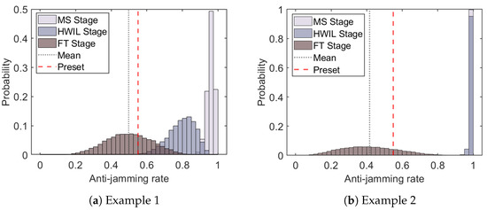
Figure 10.
Probability distributions of the anti-jamming rate at a fixed SIR value of 7.2 after fusing samples from each stage. Due to the presence of systematic errors, the fusion model at the MS and HWIL stages yields overconfident probability distributions, especially for the second example, which assigns a probability near 1 for an anti-jamming rate of 1 at this SIR value. However, after incorporating the FT stage samples, the fusion results provide a more realistic probability distribution, with the true anti-jamming rate value closer to the mean of the predicted distribution.
3.3. Comparison with the Other Fusion Models
In addition to the typical example discussed in the previous section, we conduct multiple repeated fusion processes using different random number generators, which demonstrates the robustness of our logistic fusion model. The predictions for generally exhibit good accuracy.
To further validate the effectiveness of our approach, we compare our results with other fusion models. The BETA distribution fusion model (BDF) is a multi-stage radar anti-jamming effect fusion evaluation method [22]. It is commonly used to handle binary data (0 and 1, representing failure and success, respectively). While the BDF model is also a Bayesian fusion model, it focuses solely on the success or failure of radar anti-jamming results for a single SIR value.
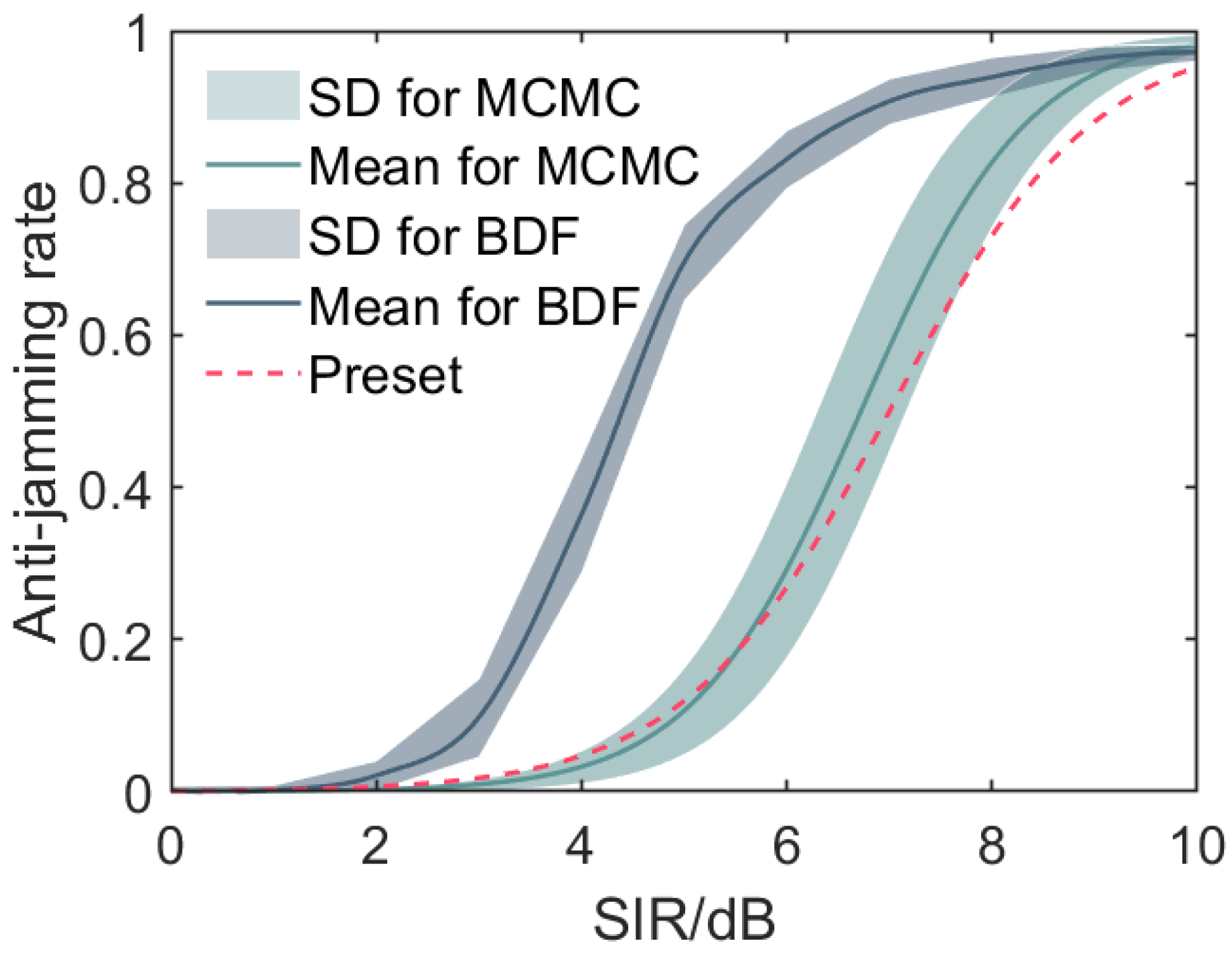
Figure 11 illustrates the fusion curve obtained by our logistic fusion model and the BDF model after 50 repetitions. With the previously preset system errors and following the data generation scheme, we generate 5, 15 and 25 samples for each SIR value across the different stages (MS, HWIL, and FT, respectively).
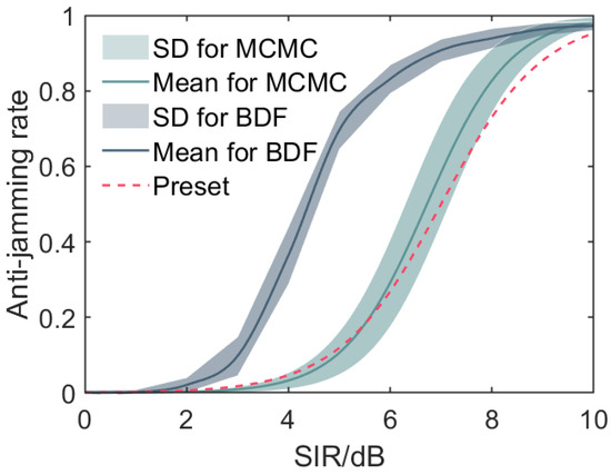
Figure 11.
Comparison of the anti-jamming rate fusion curves obtained from the proposed logistic fusion model (MCMC), the BETA distribution fusion model (BDF), and the preset true values after 50 repetitions. The solid lines represent the mean fusion curves, while the shaded regions indicate the standard deviations. The logistic fusion curve more closely follows the preset curve, demonstrating its superior performance in accurately estimating the anti-jamming rate across the SIR range. In contrast, the BDF model’s fusion curve deviates more substantially from the preset curve. The improved accuracy of our model can be attributed to its ability to leverage the intrinsic relationship between the SIR and anti-jamming results as well as its incorporation of data from multiple stages with varying reliability levels through the Bayesian fusion framework.
As evident from Figure 11, the fusion line obtained by our logistic fusion model exhibits superior predictive capabilities compared to the BDF model, more closely approaching the preset true line. The shaded regions around the fusion curves represent the standard deviations, providing insights into the variability and uncertainty associated with each model’s predictions.
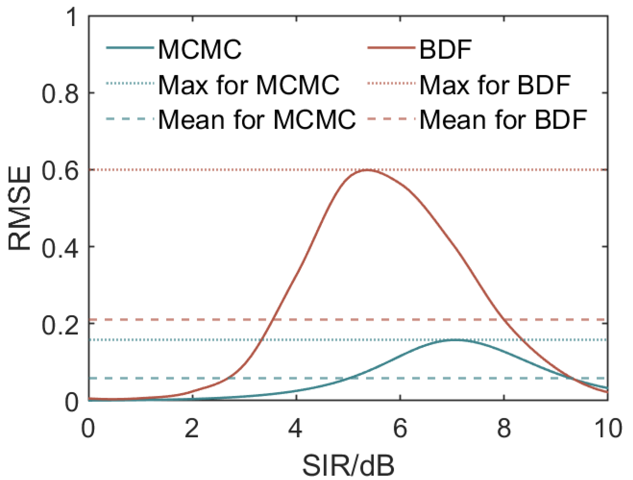
To quantify the stability of the fusion results, we employ the RMSE as an evaluation metric [22]. After 50 repetitions, our logistic fusion model achieves a significantly lower RMSE (, with a maximum value of ) compared to the BDF method (, with a maximum value of ), further demonstrating its effectiveness in providing fusion results closer to the real values (see Figure 12).
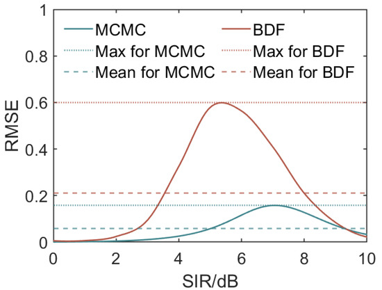
Figure 12.
RMSE comparison for different SIR values for the proposed logistic fusion model (abbreviated as MCMC) and the BETA distribution fusion model (BDF). The solid lines represent the RMSE values for the MCMC (green) and the BDF (red) over 50 repetitions. The dotted lines indicate the maximum RMSE achieved by each model across the entire SIR range, while the dashed lines represent the mean across the SIR range. It is evident that both models exhibit higher RMSE values in the inflection region of the anti-jamming rate curves.
The RMSE primarily depends on the distance between the fitted value and the preset true value, with lower values indicating better stability and accuracy. The maxima observed in Figure 12 correspond to the region around the inflection point of the logistic curve. This region is more challenging to predict due to the steep change in the logistic function. SIR values near the inflection point introduce greater variability in predicted anti-jamming performance, resulting in higher RMSE values. Intuitively, as the logistic function transitions rapidly around its inflection point, small changes in the SIR can lead to significant differences in predicted outcomes, making the prediction less accurate in this region. Consequently, the RMSE peaks around these SIR values, reflecting this inherent challenge.
It can be seen that our proposed model consistently outperforms the BDF model across almost the whole SIR range, as indicated by its lower RMSE values. The RMSE values for the logistic fusion model are notably smaller than those of the BDF model, highlighting the superior accuracy and robustness of the proposed logistic fusion approach in estimating the anti-jamming rate.
These all show that for scenarios with scarce samples, by leveraging the intrinsic relationship between the SIR and the anti-jamming results and by incorporating the MCMC method, our approach offers a more comprehensive and accurate evaluation of radar anti-jamming performance, surpassing the capabilities of the classical BDF model.
Both the BDF model and the model proposed in this paper are specifically designed to handle binary data (0 and 1, representing failure and success, respectively), utilizing Bayesian theory to estimate radar performance through the fused posterior distribution. In addition to comparing our model with the BDF model, we also compare it with other evaluation methods.
The AHP model employs expert scoring to construct a rating matrix, assigning weights to the three stages to obtain the fusion result [4]. The BayesNet model treats the three stages as leaf nodes, using the entropy weight method to determine the uncertainties of the three stages as weights for fusion [32,33,34]. The Kalman filtering model uses the data from the three stages as noisy measurements to correct the state prediction and achieve multi-stage data fusion [35].
Given that our logistic fusion model is specifically tailored to handle binary data and leverages Bayesian techniques and MCMC sampling methods, we expect it to perform better to fuse the multi-stage data. This expectation is confirmed by the results shown in Table 2, where our model achieves the best maximum, minimum, and average RMSE values.

Table 2.
Comparison of RMSEs for different fusion models.
3.4. Limitations of the Model
The proposed logistic fusion model, while effective at estimating radar anti-jamming performance by fusing data from multiple stages, exhibits certain limitations when dealing with scenarios involving a large number of samples or significant differences in systematic errors across stages.
We denote the prior distribution of and estimated by the kernel density estimation by
and we denote the likelihood function of the given observed data X by
Then, it follows from Equation (4) that
It can be seen that one potential limitation arises when the number of samples is excessively large. In our model, is formulated as the product of Bernoulli distributions, where each distribution corresponds to the anti-jamming result (success or failure) at a specific SIR level. As the number of samples increases, becomes the product of an increasing number of Bernoulli terms, so it can rapidly tend towards zero.
Another limitation arises when the systematic errors across different stages exhibit significant differences. In our model, , obtained through kernel density estimation, and are combined to derive the posterior distribution, as shown in Equation (8). If the systematic errors for different stages vary substantially, the prior distribution and the likelihood function may differ significantly, leading to a very small product value, potentially approaching the minimum representable value in floating-point arithmetic (e.g., approximately for double precision).
In such cases, the MCMC progression may fail. This limitation highlights the importance of properly accounting for and mitigating the systematic errors across different stages to ensure the successful fusion of data using the proposed model. The study of mitigating systematic errors may be explored in future research.
4. Conclusions
Faced with the challenge of limited radar anti-jamming data for performance evaluation, this paper proposes a logistic fusion model capable of fusing data from multiple stages, including MS, HWIL, and FT. By iteratively applying Bayesian fusion techniques, we obtain the posterior distributions of the parameters and in the logistic regression model, with the priors estimated through kernel function fitting.
The fusion model capitalizes on the intrinsic relationship between the SIR and the anti-jamming results, allowing for the inherent fusion of data across different SIR values in addition to different stages. Our analysis reveals that the predicted distributions of , representing the growth rate, and , representing the SIR threshold delineating success or failure (the inflection point of the logistic curve), serve as relatively accurate reflections of their true values.
From the probability distributions of and , the logistic fusion model not only provides the mean value of the radar anti-jamming rate but also a comprehensive probability distribution, offering a more nuanced understanding of the performance. Through 50 repetitions of the fusion process and comparison with other fusion models, our approach demonstrates superior fusion results. In a typical example studied in our paper, our method achieved an RMSE of 0.0552, which is significantly lower than the 0.2112 RMSE of the classical BDF model.
However, two key limitations of the proposed model should be noted. Firstly, when dealing with an excessively large number of samples, the likelihood function may have a very small value, leading to numerical instabilities during the MCMC sampling process. Secondly, if systematic errors across different data stages exhibit significant variations, the prior distribution and likelihood function may differ substantially, leading to a very small product value. These very small values may potentially approach the minimum representable value in floating-point arithmetic, where MCMC progression cannot be conducted. Hence, we anticipate the development of error-revising techniques to refine the data samples from the three stages, which will be explored in future research endeavors.
Additionally, future work will focus on implementing and testing the proposed anti-jamming algorithm on an embedded platform to validate its real-time performance and ensure its practical applicability. We also aim to enhance the generalization ability of our evaluation methods by incorporating a dataset comprising real experimental data in future testing.
In summary, the proposed logistic fusion model offers a comprehensive and robust approach to evaluating radar anti-jamming performance and aims at scenarios where data scarcity is a significant challenge. By applying Bayesian fusion and the MCMC sampling technique, our model fuses data across different SIR values and test stages. Our model transcends the constraints of single-point estimates and captures the full spectrum of potential outcomes through the derived posterior distributions, enriching our insights into the variability and uncertainty associated with the anti-jamming rate. This capability is particularly valuable when dealing with limited field test data, as the fusion process can effectively incorporate information from more abundant but less reliable sources, such as those from the MS and HWIL stages, to enhance the overall accuracy and robustness of the performance evaluation.
Author Contributions
Conceptualization, L.Z. and X.D.; Methodology, L.Z. and L.Y.; Software, L.Z. and L.Y.; Validation, Z.W.; Formal analysis, L.Z. and X.D.; Investigation, L.Y.; Resources, L.Y.; Data curation, X.D.; Writing—original draft preparation, L.Z.; Writing—review and editing, L.Y. and X.D.; Visualization, L.Z.; Supervision, Z.W. and X.D.; Project administration, L.Y.; Funding acquisition, L.Y. All authors have read and agreed to the published version of the manuscript.
Funding
This research was funded by the National Natural Science Foundation of China [No. 12101608] and by NSAF Joint Fund [No. U2230208].
Data Availability Statement
The original contributions presented in the study are included in the article, further inquiries can be directed to the corresponding author.
Acknowledgments
The authors would like to thank the anonymous referees for their suggestions and comments.
Conflicts of Interest
The authors declare no conflicts of interest.
Abbreviations
The following abbreviations are used in this manuscript:
| SIR | Signal-to-interference ratio |
| MCMC | Monte Carlo Markov chain |
| MS | Mathematical simulation |
| HWIL | Hardware-in-the-loop |
| FT | Field test |
| ACF | Autocorrelation function |
| ROC | Receiver operating characteristic |
| TPR | True positive rate |
| FPR | False positive rate |
| AUC | Area under the ROC curve |
| BDF | Beta distribution fusion |
| RMSE | Root mean square error |
References
- Claassen, G.; du Plessis, W.P. Time-Interleaved Noise Jamming. IEEE Trans. Aerosp. Electron. Syst. 2023, 59, 3359–3367. [Google Scholar] [CrossRef]
- Wei, J.; Wei, Y.; Yu, L.; Xu, R. Radar Anti-Jamming Decision-Making Method Based on DDPG-MADDPG Algorithm. Remote Sens. 2023, 15, 4046. [Google Scholar] [CrossRef]
- Pourranjbar, A.; Kaddoum, G.; Aghababaiyan, K. Deceiving-Based Anti-Jamming Against Single-Tone and Multitone Reactive Jammers. IEEE Trans. Commun. 2022, 70, 6133–6148. [Google Scholar] [CrossRef]
- Liu, X.; Yang, J.; Lu, J.; Liu, G.; Geng, Z. Application of AHP and D-S evidential theory in radar seeker anti-interference performance evaluation. J. Eng. 2019, 2019, 7977–7980. [Google Scholar] [CrossRef]
- Shuang, B.; Jun, H.; Zhiyong, N. Research on Evaluation Method of Radar Anti-jamming Effectiveness Based on Experimental Big Data. In Proceedings of the 2020 6th International Conference on Big Data and Information Analytics (BigDIA), Shenzhen, China, 4–6 December 2020; pp. 392–395. [Google Scholar] [CrossRef]
- Sun, H.; Xie, X. Threat evaluation method of warships formation air defense based on AR(p)-DITOPSIS. J. Syst. Eng. Electron. 2019, 30, 297–307. [Google Scholar]
- Yang, M.; Chen, J.; Niu, Y. An evaluation method of anti-jamming capability to communication system based on cloud-evidence theory. In Proceedings of the 2017 First International Conference on Electronics Instrumentation & Information Systems (EIIS), Harbin, China, 3–5 June 2017; pp. 1–5. [Google Scholar] [CrossRef]
- Bu, F.; He, J.; Li, H.; Fu, Q. Radar seeker anti-jamming performance prediction and evaluation method based on the improved grey wolf optimizer algorithm and support vector machine. In Proceedings of the 2020 IEEE 3rd International Conference on Electronics Technology (ICET), Chengdu, China, 8–12 May 2020; IEEE: Piscataway, NJ, USA, 2020; pp. 704–710. [Google Scholar]
- Deting, H.; Zongfeng, Q.; Teng, J.; Minpeng, Z. Effectiveness evaluation method for warning radar in jamming environment. In Proceedings of the 2018 Chinese Control And Decision Conference (CCDC), Shenyang, China, 9–11 June 2018; pp. 1755–1760. [Google Scholar]
- Li, C.; Liu, J.; Liu, X.; Kang, X.; Li, S. Combining Time-Series Variation Modeling and Fuzzy Spatiotemporal Feature Fusion: A novel Approach for unsupervised Flood Mapping using Dual-polarized Sentinel-1 SAR Images. IEEE Trans. Geosci. Remote Sens. 2023, 61, 1–15. [Google Scholar] [CrossRef]
- Peng, J.; Sun, W.; Li, H.C.; Li, W.; Meng, X.; Ge, C.; Du, Q. Low-rank and sparse representation for hyperspectral image processing: A review. IEEE Geosci. Remote Sens. Mag. 2021, 10, 10–43. [Google Scholar] [CrossRef]
- Vivone, G. Multispectral and hyperspectral image fusion in remote sensing: A survey. Inf. Fusion 2023, 89, 405–417. [Google Scholar] [CrossRef]
- Shiraki, N.; Honma, N.; Murata, K.; Nakayama, T.; Iizuka, S. Experimental Evaluation of Multi-Target Localization Accuracy Using Multistatic MIMO Radar. IEEE Sens. J. 2023, 23, 28863–28871. [Google Scholar] [CrossRef]
- Mahler, R.P. Advances in Statistical Multisource-Multitarget Information Fusion; Artech House: Norwood, MA, USA, 2014. [Google Scholar]
- Yang, Y.; Da, K.; Zhu, Y.; Xiang, S.; Fu, Q. Consensus based target tracking against deception jamming in distributed radar networks. IET Radar Sonar Navig. 2023, 17, 683–700. [Google Scholar] [CrossRef]
- Zhao, S.; Zhang, L.; Zhou, Y.; Liu, N.; Liu, J. Discrimination of active false targets in multistatic radar using spatial scattering properties. IET Radar Sonar Navig. 2016, 10, 817–826. [Google Scholar] [CrossRef]
- Ling, Q.; Huang, P.; Wang, D.; Xu, H.; Wang, L.; Liu, X.; Liao, G.; Sun, Y. Range Deception Jamming Performance Evaluation for Moving Targets in a Ground-Based Radar Network. Electronics 2023, 12, 1614. [Google Scholar] [CrossRef]
- Liu, X.; Yang, J.; Hou, B.; Lu, J.; Yao, Z. Radar seeker performance evaluation based on information fusion method. SN Appl. Sci. 2020, 2, 674. [Google Scholar] [CrossRef]
- Yang, C.; Feng, L.; Zhang, H.; He, S.; Shi, Z. A novel data fusion algorithm to combat false data injection attacks in networked radar systems. IEEE Trans. Signal Inf. Process. Networks 2018, 4, 125–136. [Google Scholar] [CrossRef]
- Qiao, S.; Fan, Y.; Zhang, H. An Improved Multi-Radar Track Weighted Data Fusion Algorithm. In Proceedings of the 2023 42nd Chinese Control Conference (CCC), Tianjin, China, 24–26 July 2023; pp. 3152–3156. [Google Scholar] [CrossRef]
- Han, L.; Ning, Q.; Chen, B.; Lei, Y.; Zhou, X. Ground threat evaluation and jamming allocation model with Markov chain for aircraft. IET Radar, Sonar Navig. 2020, 14, 1039–1045. [Google Scholar] [CrossRef]
- Zhao, L.; Yan, L.; Duan, X.; Wang, Z. A Bayesian Multistage Fusion Model for Radar Antijamming Performance Evaluation. IEEE Trans. Aerosp. Electron. Syst. 2024, 60, 729–740. [Google Scholar] [CrossRef]
- Seng, C.H.; Bouzerdoum, A.; Amin, M.G.; Phung, S.L. Two-Stage Fuzzy Fusion with Applications to Through-the-Wall Radar Imaging. IEEE Geosci. Remote Sens. Lett. 2012, 10, 687–691. [Google Scholar] [CrossRef]
- Molin, R.D.; Rosa, R.A.; Bayer, F.M.; Pettersson, M.I.; Machado, R. A Change Detection Algorithm for Sar Images Based on Logistic Regression. In Proceedings of the IGARSS 2019—2019 IEEE International Geoscience and Remote Sensing Symposium, Yokohama, Japan, 28 July–2 August 2019; IEEE: Piscataway, NJ, USA, 2019; pp. 1514–1517. [Google Scholar]
- Shao, F.; Xing, H. Logistic regression prediction based on fractal characteristics of sea surface targets. In Proceedings of the 2019 14th IEEE International Conference on Electronic Measurement & Instruments (ICEMI), Changsha, China, 1–3 November 2019; IEEE: Piscataway, NJ, USA, 2019; pp. 545–550. [Google Scholar]
- Kou, L.; Tang, J.; Wang, Z.; Jiang, Y.; Chu, Z. An Adaptive Rainfall Estimation Algorithm for Dual-Polarization Radar. IEEE Geosci. Remote Sens. Lett. 2022, 19, 1–5. [Google Scholar] [CrossRef]
- Araveeporn, A.; Klomwises, Y. The estimated parameter of logistic regression model by Markov Chain Monte Carlo method with multicollinearity. Stat. J. IAOS 2020, 36, 1253–1259. [Google Scholar] [CrossRef]
- Al-Khairullah, N.A.; Al-Baldawi, T.H. Bayesian Computational Methods of the Logistic Regression Model. J. Phys. Conf. Ser. 2021, 1804, 012073. [Google Scholar] [CrossRef]
- van Ravenzwaaij, D.; Cassey, P.; Brown, S.D. A simple introduction to Markov Chain Monte–Carlo sampling. Psychon. Bull. Rev. 2018, 25, 143–154. [Google Scholar] [CrossRef]
- Neal, R.M. Slice sampling. Ann. Stat. 2003, 31, 705–767. [Google Scholar] [CrossRef]
- Epanechnikov, V.A. Non-Parametric Estimation of a Multivariate Probability Density. Theory Probab. Its Appl. 1969, 14, 153–158. [Google Scholar] [CrossRef]
- Joo, H.; Choi, C.; Kim, J.; Kim, D.; Kim, S.; Kim, H.S. A Bayesian Network-Based Integrated for Flood Risk Assessment (InFRA). Sustainability 2019, 11, 3733. [Google Scholar] [CrossRef]
- Zheng, Y.J. Research on combat effectiveness evaluation of radar EW system based on Bayesian network. Adv. Mater. Res. 2011, 204, 1697–1700. [Google Scholar] [CrossRef]
- Pearl, J. Probabilistic Reasoning in Intelligent Systems: Networks of Plausible Inference; Elsevier: Amsterdam, The Netherlands, 2014. [Google Scholar]
- Hao, H.; Duan, Z. Tracking With Sequentially Fused Radar and Acoustic Sensor Data With Propagation Delay. IEEE Sens. J. 2023, 23, 7345–7361. [Google Scholar] [CrossRef]
- Saaty, R.W. The analytic hierarchy process—What it is and how it is used. Math. Model. 1987, 9, 161–176. [Google Scholar] [CrossRef]
Disclaimer/Publisher’s Note: The statements, opinions and data contained in all publications are solely those of the individual author(s) and contributor(s) and not of MDPI and/or the editor(s). MDPI and/or the editor(s) disclaim responsibility for any injury to people or property resulting from any ideas, methods, instructions or products referred to in the content. |
© 2024 by the authors. Licensee MDPI, Basel, Switzerland. This article is an open access article distributed under the terms and conditions of the Creative Commons Attribution (CC BY) license (https://creativecommons.org/licenses/by/4.0/).

