Technical Note

An Improved Average Acceleration Approach of Modelling Earth Gravity Field Based on K-Band Range-Rate Observations

School of Survey and Mapping, Information and Engineering University, Zhengzhou 450001, China
*
Author to whom correspondence should be addressed.
Remote Sens. 2024, 16(17), 3172; https://doi.org/10.3390/rs16173172
Submission received: 13 June 2024 / Revised: 6 August 2024 / Accepted: 13 August 2024 / Published: 28 August 2024
(This article belongs to the Section Satellite Missions for Earth and Planetary Exploration)

Abstract

:
The conventional average acceleration approach relies on K-band range observation, containing an unknown bias, which leads to possible degradation of the precision of Earth’s gravity field modelling. It also suffers from correlated errors caused by three-point numerical differentiation. In this study, an improved approach is proposed that makes use of K-band range-rate observations instead and overcoming the influence of correlated errors by introducing a whitening filter. GRACE-Follow On data spanning the period from January 2019 to December 2022 were processed by the proposed approach and a series of time-varying gravity field models was derived, referred to as SSM-AAA-GFO in this paper. This model series is compared comprehensively with three official model series. Results demonstrate that all model series are highly coincident below degree 30 and reflect similar time-varying gravity field signals in both large and small basins. After filtering, SSM-AAA-GFO shows uncertainty, in the form of equivalent water height below 2.5 cm, which is comparable with three official model series. The comparison results confirm the effectiveness of the proposed approach for precisely modelling a time-varying gravity field based on K-band range-rate observations.

1. Introduction

Earth’s gravity field reflects the distribution of Earth’s mass below and upon its surface. The time-varying information of Earth’s gravity field usually associates with geological, climatological and oceanological events, such as earthquakes, floods and rising of sea-levels. Thus, by monitoring Earth’s gravity field, the global-scale mass changes within the Earth’s system can be discovered and their connections with those events can be revealed. To achieve the above goals, the Gravity Recovery and Climate Experiment (GRACE) mission was launched in 2002, consisting of two satellites with about 500 km altitude, inclination of 89.5° and 220 km separation [1]. Over the time span of 15 years, GRACE has provided 163 monthly solutions of the time-varying gravity field (TVG) enabling the quantification of mass redistributions caused by terrestrial water storage varying, glaciers and ice sheets melting and glacial-isostatic adjustment processes [2]. Due to the tremendous success of GRACE data in many Earth science disciplines, the GRACE-Follow On mission (GRACE-FO) was approved to be implemented [3]. And, in May 2018, twin satellites constituting the constellation of the GRACE-FO mission were launched and have operated up to now. To ensure consistency with the GRACE mission, a heritage architecture similar to GRACE was chosen together with several instrumental improvements. Moreover, a joint laser ranging interferometer (LRI) was mounted to demonstrate its effectiveness in improving low–low satellite-to-satellite tracking (SST-LL) measurement performance [4].
Modelling the TVG is required for extracting the time-varying information of Earth’s gravity field from satellite observations. Several approaches, therefore, were developed and successfully applied to the GRACE mission, e.g., the classical variational approach [5,6], the short arc approach [7,8] and the energy balance approach [9,10]. The average acceleration approach, proposed by Ditmar et al. [11,12] and developed by Liu et al. [13], was also used for processing observations from the CHAllenging Minisatellite Payload (CHAMP) [14], the GRACE [13] and the Gravity Field and Steady-State Ocean Circulation Explorer (GOCE) [15,16] missions and was applied to generating the DTM model series. This approach regards the second order differentiation of satellite positions at three adjacent epochs as the pseudo-observation in the case of modelling the TVG based on high–low satellite-to-satellite tracking (SST-HL) like the CHAMP mission. In the case of SST-LL, e.g., the GRACE mission, the weighted combination of K-band range observations at three adjacent epochs usually offers the major part of gravity field information as the pseudo-observation. The K-band range observation, however, contains an unknown constant bias within a continuous measurement leading the distortion of the TVG modelling. Additionally, the computation of the weighted combination of K-band range observations needs the unit vector in the line-of-sight (LOS) direction, which is computed by position observations of the two satellites, making it contaminated by position errors. To deal with these problems, Liu et al. [13] made use of the pure dynamic orbit instead of the kinematic orbit and estimated the K-band range bias by the position differences of the two satellites. But estimating the K-band range bias from satellite positions contaminates high-precision K-band ranging measurements since the precision of positioning is only several centimeters and the precision of K-band ranging is higher than 1 μ m. Chen et al. [17] subtracts two pseudo-observations at adjacent epochs for eliminating the K-band range bias possibly introducing some correlations between epochs. Shen et al. [18] made use of Cowell, KSG, and Adams integrators along with estimating initial orbital position and velocity vectors and incorporated range-rate data into gravity field estimation. However, Shen’s method is more like the combination of the dynamic approach and the acceleration approach.
In this study, another way to overcome deficiencies of the conventional approach is proposed in which the correlation errors caused by numerical differentiation is decorrelated by whitening filtering and a new formulation is derived for the utilization of K-band range-rate observations. Thereout, an improved average acceleration approach is proposed and used for processing the GRACE-FO data for producing a new TVG model series, referred to as SSM-AAA-GFO. The subsequent sections of this article are structured as follows: In Section 2, the theoretical model of the proposed approach is introduced. In Section 3, details of GRACE-FO data processing are described and results of comprehensive comparisons between SSM-AAA-GFO and three official models, i.e., CSR RL06, JPL RL06 and GFZ RL06, are shown in Section 4. Conclusions are made in Section 5.

2. Methodology

The average acceleration approach links the second order numerical differentiation of the satellite positions at three adjacent epochs with its weighted average acceleration by
r t + Δ t 2 r t + r t Δ t Δ t 2 = 1 Δ t Δ t Δ t Δ t s Δ t f r t + s , u d s
where r t represents the satellite position at epoch t, Δ t denotes the time interval between two adjacent epochs, f r t , u describes the total acceleration acting on the satellite and the vector u consists of force parameters, including the spherical harmonic coefficients, the accelerometer bias, etc. After linearizing the total acceleration f r t , u , discretizing the integration and introducing position observations associated with their errors, Equation (1) can be reformulated as
r ^ t + Δ t 2 r ^ t + r ^ t Δ t Δ t 2 + Δ r ^ t + Δ t 2 Δ r ^ t + Δ r ^ t Δ t Δ t 2 = 1 Δ t s = Δ t Δ t k s Δ t s Δ t f r ^ t + s , u ˜ Δ s + 1 Δ t s = Δ t Δ t k s Δ t s Δ t f r ^ t + s , u ˜ u Δ s δ u + 1 Δ t s = Δ t Δ t k s Δ t s Δ t f r ^ t + s , u ˜ r ^ t + s Δ s Δ r ^ t + s + ε t
with the hat labelling the elements gained from measurements, the tilde labelling the elements introduced as references, r ^ t and Δ r ^ t denoting the observed satellite position and its error at epoch t, respectively, Δ s denoting the integration step, k s denoting the discrete integration parameter, u ˜ meaning the reference value of u and δ u meaning its correct vector and ε t denoting the omit error caused by the linearization and the discretization. Since Equation (2) can be established at every epoch besides at the beginning and the end, neglecting the omit error, there can be
D r ^ + Δ r ^ = KF + KA δ u + KG Δ r ^ ; D = 1 Δ t 2 I 3 × 3 2 I 3 × 3 I 3 × 3 I 3 × 3 2 I 3 × 3 I 3 × 3 ; r ^ = r ^ T t 1 r ^ T t n T ; Δ r ^ = Δ r ^ T t 1 Δ r ^ T t n T ; F = f r ^ t 1 , u ˜ f r ^ t n , u ˜ ; A = f r ^ t 1 , u ˜ u f r ^ t n , u ˜ u ; G = f r ^ t 1 , u ˜ r ^ t 1 f r ^ t n , u ˜ r ^ t n
with n denoting the number of observations within an arc, matrix K consisting of discrete integration parameters k s and t 1 and t n denoting the start epoch and the end epoch within an arc, respectively. The inter-epoch correlated errors are introduced because of the numerical differentiation and the numerical integration. By introducing two pseudo-observations as
r t 1 = r ^ t 1 + Δ r ^ t 1 r t n = r ^ t n + Δ r ^ t n
into Equation (3), the correlated errors can be decorrelated by the filter matrix
C = I 3 × 3 0 3 × 3 ( n 2 ) 0 3 × 3 0 3 ( n 2 ) × 3 0 3 ( n 2 ) × 3 ( n 2 ) 0 3 ( n 2 ) × 3 0 3 × 3 0 3 × 3 ( n 2 ) I 3 × 3 + 0 3 × 3 n D 0 3 × 3 n 0 3 × 3 n K 0 3 × 3 n G 1
with matrix I being an identity matrix and matrix 0 being a zero matrix. Then, Equation (3) can be transformed into
Δ r ^ = CK A δ u + CK F CD r ^ ; D = 0 3 × 3 n D 0 3 × 3 n ; K = 0 3 × 3 n K 0 3 × 3 n
For the utilization of K-band range-rate observations, a new formulation has to been introduced that is formulated as
r ˙ t = r t + Δ t r t Δ t 2 Δ t 1 2 Δ t Δ t Δ t h s f r t + s , u d s ; h s = s Δ t     , Δ t < s 0 Δ t s , 0 < s < Δ t
And the velocity difference between the two satellites can be interpreted as
r ˙ 12 t = r 12 t + Δ t r 12 t Δ t 2 Δ t 1 2 Δ t Δ t Δ t h s f 2 r 2 t + s , u f 1 r 1 t + s , u d s
where the subscript 1 and 2 labelling the element belonging to the leading satellite and the trailing satellite, respectively, and the subscript 12 denoting the subtraction between elements of the two satellites. By multiplying the unit vector, e 12 , in the LOS direction and the velocity difference vector, we obtain
ρ ˙ t = e 12 T t r ˙ 12 t = e 12 T r 12 t + Δ t r 12 t Δ t 2 Δ t 1 2 Δ t e 12 T Δ t Δ t h s f 2 r 2 t + s , u f 1 r 1 t + s , u d s
with ρ ˙ t denoting the K-band range-rate at epoch t. Furthermore, taking into consideration the observed position errors and discretizing the integration, Equation (9) is reformulated as
˙ ^ ρ t + Δ ˙ ^ ρ t = e ^ 12 T t ˙ ¯ r 12 t + e ^ 12 T t ˙ ¯ r 12 t u δ u + e ^ 12 T t ˙ ¯ r 12 t r 1 t Δ r 1 t + e ^ 12 T t ˙ ¯ r 12 t r 2 t Δ r 2 t ˙ ¯ r 12 t = r ^ 12 t + Δ t r ^ 12 t Δ t 2 Δ t 1 2 Δ t s = Δ t Δ t k s h s f 2 r ^ 2 t + s , u ˜ f 1 r ^ 1 t + s , u ˜ Δ s
where e ^ 12 t is the unit vector in the LOS direction computed by observed satellite positions at epoch t and ˙ ¯ r t denotes the integral velocity. Equation (6) can be substituted into this equation. Equations (6) and (10) are the basic formulas of the improved average acceleration approach, which decorrelates correlated errors caused by numerical differentiation and integration by filtering matrix C of Equation (5) and introduces K-band range-rate observations by Equation (10).

3. Data Processing

By exploiting the improved average acceleration approach, the GRACE-FO observation data, spanning the period from January 2019 to December 2022, were processed. Table 1 shows the details of data processing. The observation data, including reduced dynamic orbits, accelerometer observations, rotation quaternions, and K-band range-rates, are provided by the Jet Propulsion Laboratory (JPL) as level-1B products in release 4. All data are down-sampled to 0.2 Hz for matching the sample rate of the K-band range-rate data. For data gaps shorter than 3 min, data packing is implemented by the nine-nodes Lagrange’s interpolation except for the K-band range-rate data set as it contains the basic observations for gravity field modelling. Outliers of accelerometer observations are detected by a daily median-based threshold with a value of 1 μ m/s2, which is also adopted by the data processing for deriving the AIUB-G3P model series [19]. The K-band range-rate data are compared with nominal values computed by reduced dynamic orbits and are screened according to their differences obeying the 5-sigma criterion.
The GOCO06s model [20], both with its static component and temporal component, is chosen to be the reference Earth gravity field model. The periodic variations of ocean tides are modelled by the FES2014b model [21]. The effects of high-frequency variations of ocean and atmosphere are eliminated by the AOD1B products in release version 6 [22] provided by the GeoForschungsZentrum Potsdam (GFZ). Precise positions of the solar system bodies are referred to the DE430 ephemeris [23]. The three-body perturbation is computed with the mass point approximation and the consideration of J2 effects of Earth. Adopting the recommendations of the IERS 2010 convention [24], the effects of the Earth tide, the pole tide and the general relativity are taken into consideration.
Table 1. Data processing details.
Observation Data
GNV1BReduced dynamic orbit data with sample rate of 1 Hz
SCA1BRotation quaternion from inertial frame to GRACE science reference frame with sample rate of 1 Hz
ACT1BTransplanted non-conservative acceleration data with sample rate of 1 Hz
KBR1BK-band ranging data, including inter-satellite range, its first and second order derivatives and corresponding phase center and light-time corrections, with sample rate of 0.2 Hz
Back ground model
Earth’s gravity fieldGOCO06s model with static component up to degree and order 300 and temporal component up to degree and order 200
Ocean tideFES2014b model up to degree and order 180 with 34 major tidal constituents and 361 minor tidal constituents
N-body PerturbationJPL DE430 planetary ephemerides, consider Sun, Moon, Venus, Mars, Saturn and Jupiter, direct and indirect J2 effect
Solid earth TideIERS Conventions 2010, include frequency independent term, frequency dependent term and permanent tide
Solid earth pole tideIERS Conventions 2010
Ocean pole tideDesai [25], up to degree and order 180
Atmospheric and oceanic variabilityAOD1B RL06, linear interpolation, include 12 atmosphere tidal constituents
General relativistic effectIERS Conventions 2010
Estimated parameter
Spherical harmonic coefficientsComplete to degree and order 96
Accelerometer calibration parametersBiases, once per revolution (1.5 h), include biases in along-track, cross-track and radial direction; Scales, once per day, full scale matrix
K-band ranging empirical parametersBias and slope, once per half revolution; One cycle-per-revolution (1CPR) components, once per revolution
Spherical harmonic coefficients up to degree 96 are estimated every calendric month except in February 2019 when data from an additional 10 days of measurements are incorporated because of a 12-day data gap. For the accelerometer calibration, the accelerometer bias of each satellite is estimated every 1.5 h at each axis and elements of a full scale matrix is estimated every day for each satellite. A set of empirical parameters are estimated per orbit revolution for assimilating low-frequency errors brought by the K-band ranging measurement noise and the deficiencies of background models. According to the experimental result shown in Figure 1, an arc length of 3 h is chosen for balancing the computation burden and the precision of Earth gravity field modelling.
The estimation of unknown parameters is implemented obeying the least squares criterion. The prior variances of position errors and K-band range-rate errors are 2 cm and 0.1 μ m/s, respectively; however, position observations are empirically down-weighted by a factor of 0.2 for better estimation of spherical harmonic coefficients. Before inverting the final normal equations, arc-wise parameters are pre-eliminated, and the normal equations for each arc are accumulated. Since data screening can not screen out all outliers before the estimation, data are screened once again, based on posterior residuals, after the first estimation. A threshold of four times the root mean square (RMS) of posterior residuals is adopted. Next, the second estimation is conducted based on twice-screened data for gravity field modelling.

4. Results

By processing the GRACE-FO data, a model series consisting of 48 monthly TVG models has been derived and it is referred to as SSM-AAA-GFO in this paper for the convenience of description. To evaluate the precision of the derived model series, comprehensive comparisons have been made between it and the models provided by the Center for Space Research at University of Texas (CSR), the GFZ and the JPL, respectively, in both the spectral domain and spatial domain. These models are released as the GRACE-FO level-2 data products in release version 06, called CSR RL06, GFZ RL06 and JPL RL06.

4.1. Spectral Analysis

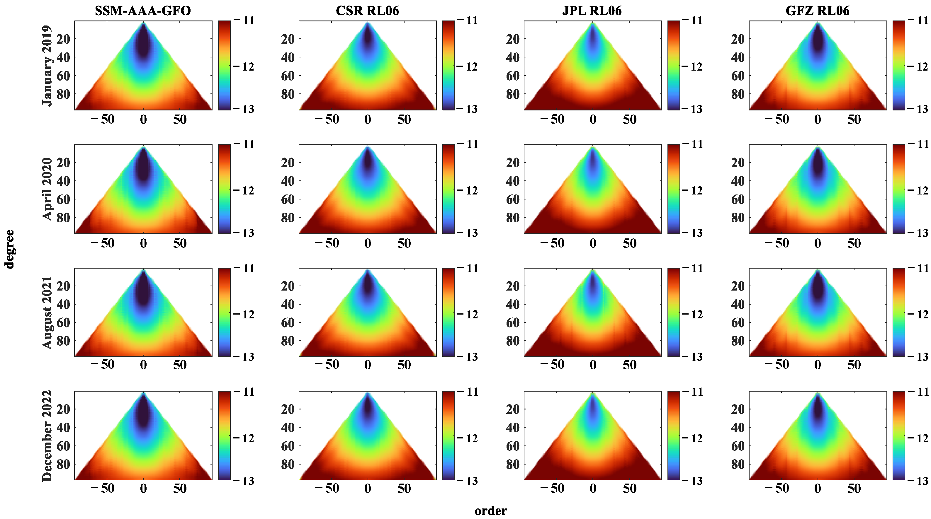
For making comparisons in the spectral domain, the information from the process of estimation itself should be taken into consideration. Figure 2 illustrates posterior variances of estimated spherical harmonic coefficients of each model series in several selected months. These months include January 2019, April 2020, August 2021 and December 2022, which are uniformly distributed within four years. According to Figure 2, in all selected months, SSM-AAA-GFO seems to have better inner coincidents than others as it holds the lowest values of posterior variances. From the point of view of adjustment theory, the uncertainty of estimated spherical harmonic coefficients of SSM-AAA-GFO below degree 60 and order 40 is lower than 10−12 and it is below 10−11 for most of coefficients. However, this can hardly demonstrate that SSM-AAA-GFO holds the highest accuracy among model series since the posterior variances are distorted by mismodelling of overall errors, mainly including measurement errors and back ground model uncertainty. Thus, posterior variances tend to underestimate the uncertainty of estimation results.To obtain more reasonable comparison results, the calibrated error—defined as the residual after subtracting the mean, trend, and annual and semi-annual signals from the model series at each degree and order—is computed and shown in Figure 3.
In Figure 3, the calibrated errors reflect a more realistic error level of the four model series, demonstrating precision degradation at resonance orders (multiples of 15 or 16), better estimation of near-zonal terms, and a dramatic increase in errors at high degrees. Referring to the calibrated errors, SSM-AAA-GFO performs comparably with the other three model series below order 30 with uncertainty of about 10−12. But, between order 30 and order 50, the performance of this model series is a little inferior (in certain months such as January 2019 and August 2021), demonstrating a demand for refinements of data processing strategy.
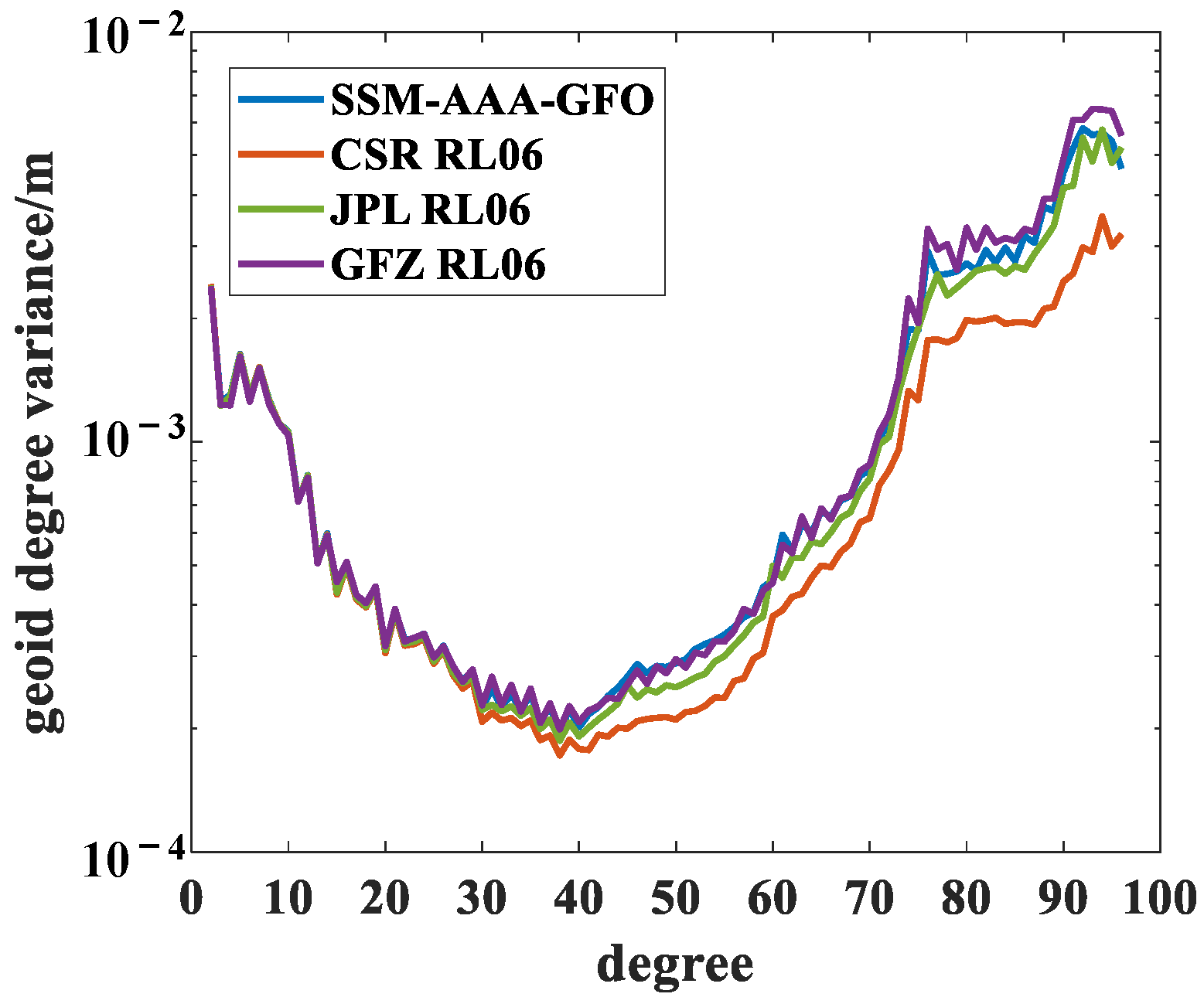
The geoid degree variance is another index for reflecting signal constants and error level of a TVG model at each degree. By referring to the EIGEN-6C4 model, geoid degree variances of each model series in selected months were computed and the temporal mean geoid degree variances of all 48 models of each series were also calculated. All results are shown in Figure 4 and Figure 5.
It is widely accepted that the signal of TVG dominates the spherical harmonic coefficients before degree 30 and, after that degree, the signal–noise rate dramatically reduces [26,27]. According to Figure 4, before degree 30, geoid degree variances of four model series are highly coincident but, after that degree, diverge gradually as the degree increases. This demonstrates that these model series contain the same signals and a different level of errors in selected months. Among four model series, CSR RL06 holds the lowest error level after degree 30, possibly because of its separate estimation of local parameters and spherical harmonic coefficients [28]. As for the other three model series, their errors are at a similar level and this inference is also confirmed by their temporal mean geoid degree variances shown in Figure 5. In January 2019 and August 2021, a higher error level of SSM-AAA-GFO between degree 30 and 60 can be seen, confirming the necessity for the refinement of the data processing strategy in certain months.

4.2. Spatial Analysis

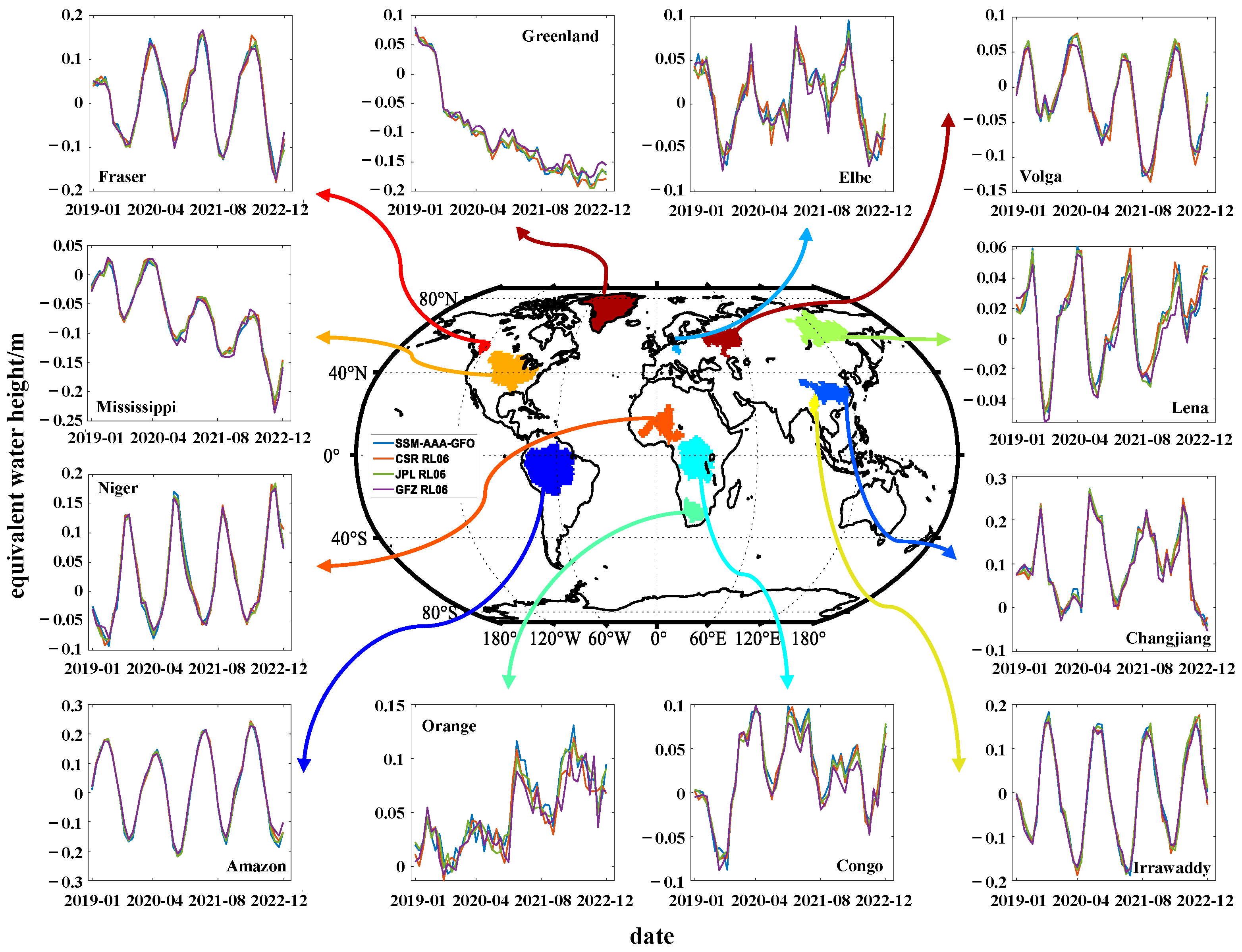
For making comparisons in the spatial domain, spherical harmonic coefficients should firstly be transformed into equivalent water height (EWH) grids. The EWH reflects the local mass variation in the form of the increase or decrease of a regional mean water thickness. All 48 models of each series, filtering by a destriping filter [29] and a Gaussian filter with 300 km radius, were transformed into global EWH grids and the temporal mean value was extracted from each grid. Figure 6 illustrates EWH grids in selected months and Figure 7 shows TVG signals in 11 representative basins in Greenland. Note that, in Figure 7, the scale of y-axes is different for displaying TVG signals in different basins for more details.
According to Figure 6, all model series reflect similar TVG signals, especially in terrestrial areas like Africa, the Amazon basin and Greenland, and the greatest differences between them are located in oceanic areas where fewer TVG signals exist. Apparent seasonal signals can be revealed in areas where the increase and the decrease of EWH happen alternately over time. However, after filtering, the north–south striping noise still exists and can be obviously distinguished from signals in oceanic areas. The consistency of TVG signals of four model series is also confirmed by Figure 7. From Figure 7, the temporal variations of EWH, computed by different model series, are highly consistent either in large basins, like the Amazon, the Mississippi and the Congo, or in small basins, like the Fraser, the Elbe and the Irrawaddy. All model series reveal the continuous ice run-off occuring in Greenland and the regular annual variation caused by the cycle of seasons in basins. However, because of differences in data processing strategies, minor divergences still exist, for example, in the Orange basin.
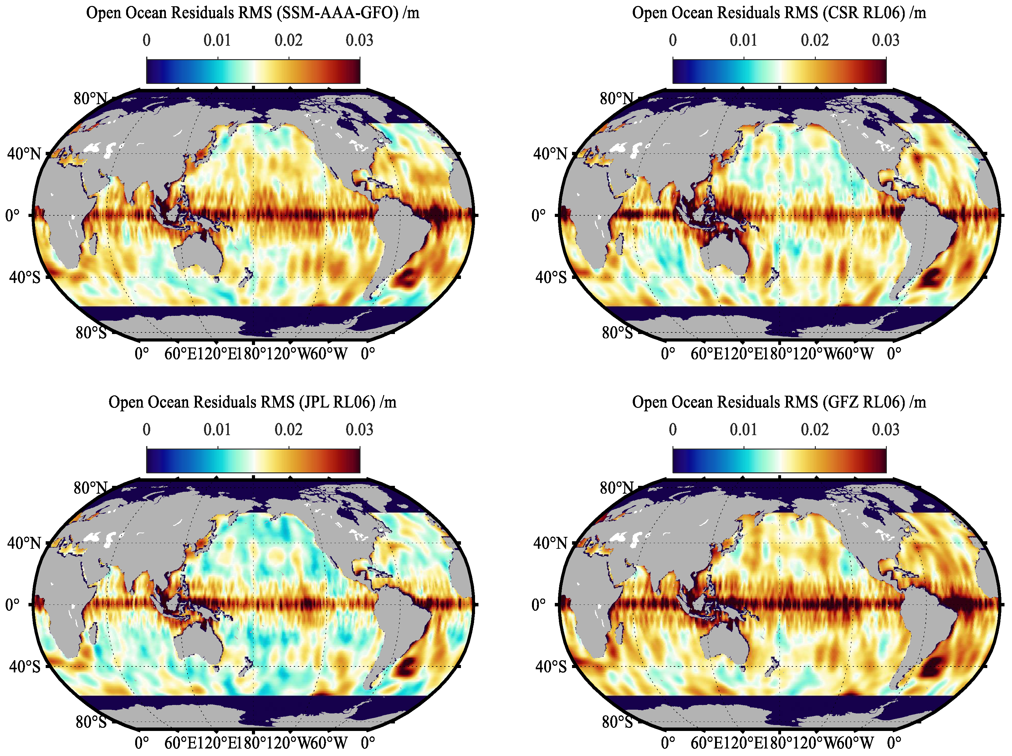
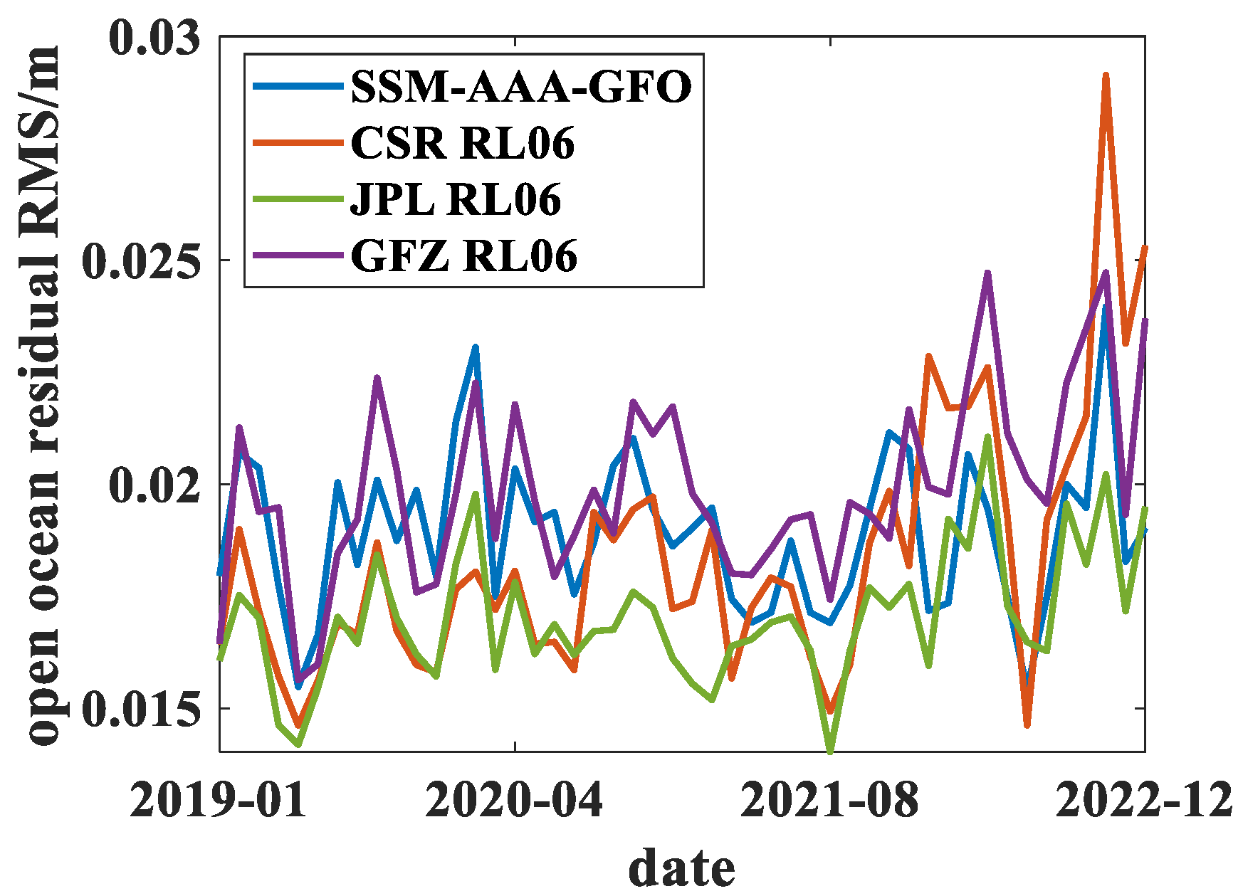
For evaluating the error level of each model series, the open ocean residuals (OORs) [30] are computed by fitting and subtracting the trend, the annual variation and the semi-annual variation from each EWH grid in oceanic areas. For avoiding the signal leakage from terrestrial areas, areas at a latitude above 70 degrees north and below 70 degrees south and areas with a distance below 300 km from the coastline are excluded from computation. OORs of all 48 models of each series were computed. For making comparisons, the RMS of OOR time series at each grid, referred to as tRMS, and the latitude-cosine-weighted RMS of global OORs in every month, referred to as wRMS, are computed. Figure 8 shows the OOR tRMS of each model series and Figure 9 shows the value of OOR wRMS in all 48 months. According to Figure 8, the value of tRMS at most grids is below 2 cm for four model series and some larger values of tRMS at grids near the equator can be attributed to the feature of destriping filtering. From Figure 9, we can know the error level of each model series month by month. The OOR wRMS of all model series in almost all considered months is below 2.5 cm except for CSR RL06 in later 2022. SSM-AAA-GFO performs comparably with other model series and JPL RL06 performs best as it holds the lowest value of OOR wRMS almost over four years. However, SSM-AAA-GFO performs a litter better than JPL RL06 in certain months in early 2022.

5. Conclusions

The conventional average acceleration approach suffers from the correlated errors caused by second-order numerical differentiation and the unknown bias of K-band range observations. An improved approach has been proposed, which decorrelates errors by introducing a whitening filter and takes the utilization of K-band range-rate through a new formulation. By exploiting the proposed approach, GRACE-FO data spanning four years have been processed and a TVG model series, SSM-AAA-GFO, has been derived. Compared with CSR RL06, GFZ RL06 and JPL RL06 model series in both spectral and spatial domain, SSM-AAA-GFO is highly consistent with these model series before degree 30 where signals take the dominant place. Both in 11 representative basins and in Greenland, all model series reflect similar TVG signals. After filtering, the uncertainty of SSM-AAA-GFO, in form of EWH, is below 2.5 cm reaching performance comparable with the other three model series. It can be confirmed that the proposed improved average acceleration approach can effectively extract gravity field signal and produce high-precision TVG models.

Author Contributions

Conceptualization, S.L. and D.F.; methodology, X.T.; software, X.T.; validation, J.F., H.W. and Z.X.; formal analysis, X.T.; investigation, H.W.; resources, J.F.; data curation, Z.X.; writing—original draft preparation, X.T.; writing—review and editing, S.L.; visualization, D.F.; supervision, S.L.; project administration, S.L.; funding acquisition, S.L. All authors have read and agreed to the published version of the manuscript.

Funding

This study is sponsored by the National Natural Science Foundation of China (42174007).

Data Availability Statement

The GRACE-FO Level 1B data in this study are freely available at ftp://isdcftp.gfz-potsdam.de (accessed on 1 January 2023). The SSM-AAA-GFO model is openly available upon reasonable request to the corresponding author.

Acknowledgments

We would like to thank JPL for providing us the GRACE-FO level-1B data. We also would like to thank Wei Feng for using the GRACE Matlab Toolbox (GRAMAT) in version 3 to conduct part of the research for this article [31].

Conflicts of Interest

The authors declare no conflicts of interest.

References

  1. Tapley, B.D.; Bettadpur, S.; Watkins, M.; Reigber, C. The gravity recovery and climate experiment: Mission overview and early results. Geophys. Res. Lett. 2004, 31, L09607. [Google Scholar] [CrossRef]
  2. Tapley, B.D.; Watkins, M.M.; Flechtner, F.; Reigber, C.; Bettadpur, S.; Rodell, M.; Sasgen, I.; Famiglietti, J.S.; Landerer, F.W.; Chambers, D.P.; et al. Contributions of GRACE to understanding climate change. Nat. Clim. Chang. 2019, 9, 358–369. [Google Scholar] [CrossRef]
  3. Flechtner, F.; Morton, P.; Watkins, M.; Webb, F. Status of the GRACE follow-on mission. In Gravity, Geoid and Height Systems; Marti, U., Ed.; Springer: Berlin, Germany, 2014; pp. 117–121. [Google Scholar]
  4. Flechtner, F.; Neumayer, K.H.; Dahle, C.; Dobslaw, H.; Fagiolini, E.; Raimondo, J.C.; Güntner, A. What can be expected from the GRACE-FO laser ranging interferometer for earth science applications? In Remote Sensing and Water Resources; Cazenave, A., Champollion, N., Benveniste, J., Chen, J., Eds.; Springer: Berlin, Germany, 2016; pp. 263–280. [Google Scholar]
  5. Zhou, H.; Zheng, L.; Li, Y.; Guo, X.; Zhou, Z.; Luo, Z. HUST-Grace2024: A new GRACE-only gravity field time series based on more than 20 years of satellite geodesy data and a hybrid processing chain. Earth Syst. Sci. Data 2024, 16, 3261–3281. [Google Scholar] [CrossRef]
  6. Zhou, H.; Luo, Z.; Zhong, B. WHU-Grace01s: A new temporal gravity field model recovered from GRACE KBRR data alone. Geod. Geodyn. 2015, 6, 316–323. [Google Scholar] [CrossRef]
  7. Chen, Q.; Shen, Y.; Zhang, X.; Hsu, H.; Chen, W.; Ju, X.; Lou, L. Monthly gravity field models derived from GRACE Level 1B data using a modified short-arc approach. J. Geophys. Res. Solid Earth 2015, 120, 1804–1819. [Google Scholar] [CrossRef]
  8. Chen, Q.; Shen, Y.; Chen, W.; Francis, O.; Zhang, X.; Chen, Q.; Li, W.; Chen, T. An optimized short-arc approach: Methodology and application to develop refined time series of Tongji-Grace2018 GRACE monthly solutions. J. Geophys. Res. Solid Earth 2019, 124, 6010–6038. [Google Scholar] [CrossRef]
  9. Shang, K.; Guo, J.; Shum, C.K.; Dai, C.; Luo, J. GRACE time-variable gravity field recovery using an improved energy balance approach. Geophys. J. Int. 2015, 203, 1773–1786. [Google Scholar] [CrossRef]
  10. Zhong, B.; Li, X.; Chen, J.; Li, Q. WHU-GRACE-GPD01s: A Series of Constrained Monthly Gravity Field Solutions Derived From GRACE-Based Geopotential Differences. Earth Space Sci. 2023, 10, e2022EA002699. [Google Scholar] [CrossRef]
  11. Ditmar, P.; Sluijs, A.V.E.V.D. A technique for modeling the Earth’s gravity field on the basis of satellite accelerations. J. Geod. 2004, 78, 12–33. [Google Scholar] [CrossRef]
  12. Ditmar, P.; Sluijs, A.V.E.V.D.; Kuznetsov, V. Modeling the Earth’s gravity field from precise satellite orbit data: The acceleration approach works! In Proceedings of the “GOCE, The Geoid and Oceanography”, Frascati, Italy, 8–10 March 2004. [Google Scholar]
  13. Liu, X.; Ditmar, P.; Siemes, C.; Slobbe, D.C.; Revtova, E.; Klees, R.; Riva, R.; Zhao, Q. DEOS Mass Transport model (DMT-1) based on GRACE satellite data: Methodology and validation. Geophys. J. Int. 2010, 181, 769–788. [Google Scholar] [CrossRef]
  14. Ditmar, P.; Kuznetsov, V.; Sluijs, A.V.E.V.D.; Schrama, E.; Klees, R. ‘DEOS_CHAMP-01C_70’: A model of the Earth’s gravity field computed from accelerations of the CHAMP satellite. J. Geod. 2006, 79, 586–601. [Google Scholar] [CrossRef]
  15. Farahani, H.H.; Ditmar, P.; Inácio, P.; Didova, O.; Gunter, B.; Klees, R.; Guo, X.; Guo, J.; Sun, Y.; Liu, X.; et al. A high resolution model of linear trend in mass variations from DMT-2: Added value of accounting for coloured noise in GRACE data. J. Geodyn. 2017, 103, 12–25. [Google Scholar] [CrossRef]
  16. Farahani, H.H.; Ditmar, P.; Klees, R.; Liu, X.; Zhao, Q.; Guo, J. The static gravity field model DGM-1S from GRACE and GOCE data: Computation, validation and an analysis of GOCE mission’s added value. J. Geod. 2013, 87, 843–867. [Google Scholar] [CrossRef]
  17. Chen, Q.; Shen, Y.; Chen, W.; Zhang, X.; Hsu, H.; Ju, X. A modified acceleration-based monthly gravity field solution from GRACE data. Geophys. J. Int. 2015, 202, 1190–1206. [Google Scholar] [CrossRef]
  18. Shen, Z.; Chen, Q.; Shen, Y. An Improved Acceleration Approach by Utilizing K-Band Range Rate Observations. Remote Sens. 2023, 15, 5260. [Google Scholar] [CrossRef]
  19. Darbeheshti, N.; Lasser, M.; Meyer, U.; Arnold, D.; Jäggi, A. AIUB-GRACE gravity field solutions for G3P: Processing strategies and instrument parameterization. Earth Syst. Sci. Data 2024, 16, 1589–1599. [Google Scholar] [CrossRef]
  20. Kvas, A.; Brockmann, J.M.; Krauss, S.; Schubert, T.; Gruber, T.; Meyer, U. GOCO06s—A satellite-only global gravity field model. Earth Syst. Sci. Data 2021, 13, 99–118. [Google Scholar] [CrossRef]
  21. Lyard, F.H.; Allain, D.J.; Cancet, M.; Carrère, L.; Picot, N. FES2014 global ocean tide atlas: Design and performance. Ocean. Sci. 2021, 17, 615–649. [Google Scholar] [CrossRef]
  22. Dobslaw, H.; Bergmann-Wolf, I.; Dill, R.; Poropat, L.; Thomas, M.; Dahle, C.; Esselborn, S.; König, R.; Flechtner, F. A new high-resolution model of non-tidal atmosphere and ocean mass variability for de-aliasing of satellite gravity observations: AOD1B RL06. Geophys. J. Int. 2017, 211, 263–269. [Google Scholar] [CrossRef]
  23. Folkner, W.M.; Williams, J.G.; Boggs, D.H.; Park, R.S.; Kuchynka, P. The Planetary and Lunar Ephemerides DE430 and DE431. Available online: https://www.google.com/url?sa=t&source=web&rct=j&opi=89978449&url=https://naif.jpl.nasa.gov/pub/naif/generic_kernels/spk/planets/de430_and_de431.pdf&ved=2ahUKEwiwoITVgoCIAxVErokEHRS6PUkQFnoECBcQAQ&usg=AOvVaw2i8bA6P-_iLhX2Hkq3rCcl (accessed on 12 August 2024).
  24. Petit, G.; Luzum, B. IERS Conventions. (No. IERS-TN-36); Bureau International Des Poids et Mesures Sevres: Sèvres, France, 2010. [Google Scholar]
  25. Desai, S.D. Observing the pole tide with satellite altimetry. J. Geophys. Res. Ocean. 2002, 107, 7-1–7-13. [Google Scholar] [CrossRef]
  26. Chen, Q.; Shen, Y.; Francis, O.; Chen, W.; Zhang, X.; Hsu, H. Tongji-Grace02s and Tongji-Grace02k: High-precision static GRACE-only global Earth’s gravity field models derived by refined data processing strategies. J. Geophys. Res. Solid Earth 2018, 123, 6111–6137. [Google Scholar] [CrossRef]
  27. Meyer, U.; Jäggi, A.; Jean, Y.; Beutler, G. AIUB-RL02: An improved time-series of monthly gravity fields from GRACE data. Geophys. J. Int. 2016, 205, 1196–1207. [Google Scholar] [CrossRef]
  28. Duan, X.J.; Guo, J.Y.; Shum, C.K.; Van Der Wal, W. On the postprocessing removal of correlated errors in GRACE temporal gravity field solutions. J. Geod. 2009, 83, 1095–1106. [Google Scholar] [CrossRef]
  29. Bettadpur, S. UTCSR level-2 processing standards document for level-2 product release 0006. GRACE Rep. 2018, 327, 742. [Google Scholar]
  30. Chen, J.; Tapley, B.; Tamisiea, M.E.; Save, H.; Wilson, C.; Bettadpur, S.; Seo, K.W. Error assessment of GRACE and GRACE follow-on mass change. J. Geophys. Res. Solid Earth 2021, 126, e2021JB022124. [Google Scholar] [CrossRef]
  31. Feng, W. GRAMAT: A comprehensive Matlab toolbox for estimating global mass variations from GRACE satellite data. Earth Sci. Inform. 2018, 12, 389–404. [Google Scholar] [CrossRef]
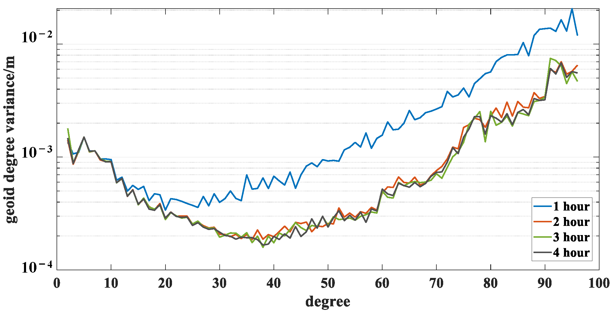
Figure 1. Geoid degree variances of Earth gravity field models adopting different arc length.
Remotesensing 16 03172 g001
Figure 2. The logarithm of posterior variances of contrastive models in selected months.
Remotesensing 16 03172 g002
Figure 3. The logarithm of calibrated errors of contrastive models in selected months.
Remotesensing 16 03172 g003
Figure 4. Geoid degree variances of contrastive models in selected months.
Remotesensing 16 03172 g004
Figure 5. Mean geoid degree variances of contrastive models over 48 months.
Remotesensing 16 03172 g005
Figure 6. Global mass variation, in the form of EWH, computed by four model series in selected months.
Remotesensing 16 03172 g006
Figure 7. Temporal variations of EWH computed by four model series in representative basins in Greenland (differences color lines for distinguishing different basins).
Remotesensing 16 03172 g007
Figure 8. The OOR tRMS of four model series all over the globe.
Remotesensing 16 03172 g008
Figure 9. The OOR wRMS of four model series over 48 months.
Remotesensing 16 03172 g009
Disclaimer/Publisher’s Note: The statements, opinions and data contained in all publications are solely those of the individual author(s) and contributor(s) and not of MDPI and/or the editor(s). MDPI and/or the editor(s) disclaim responsibility for any injury to people or property resulting from any ideas, methods, instructions or products referred to in the content.