
Assessment of Semi-Automated Techniques for Crop Mapping in Chile Based on Global Land Cover Satellite Data


Abstract
1. Introduction
2. Study Area
3. Data and Methods
3.1. Data
3.1.1. In Situ Data
3.1.2. Satellite-Based Data
Landsat 8
Sentinel-2
MODIS
ESA World Cover
Dynamic World
3.2. Methods: Agricultural Area Calculation
3.2.1. Reprojection and Filtering
3.2.2. Training Sample Selection and Classification
3.2.3. Accuracy Assessment
3.3. Work Strategy
4. Results
5. Discussion
6. Conclusions
Author Contributions
Funding
Data Availability Statement
Acknowledgments
Conflicts of Interest
Appendix A

| Class | Trees | Cropland | Urban | Grassland | Shrub | Bare |
|---|---|---|---|---|---|---|
| ED threshold | 0.06 | 0.07 | 0.10 | 0.10 | 0.05 | 0.10 |
Appendix B
| Year | 2007 | 2021 | |||||||||
|---|---|---|---|---|---|---|---|---|---|---|---|
| Commune (Area [km2]) | AS | MODIS | MODIS v2 | AS | MODIS | MODIS v2 | ESA | ESA v2 | DW | DW v2 | CONAF |
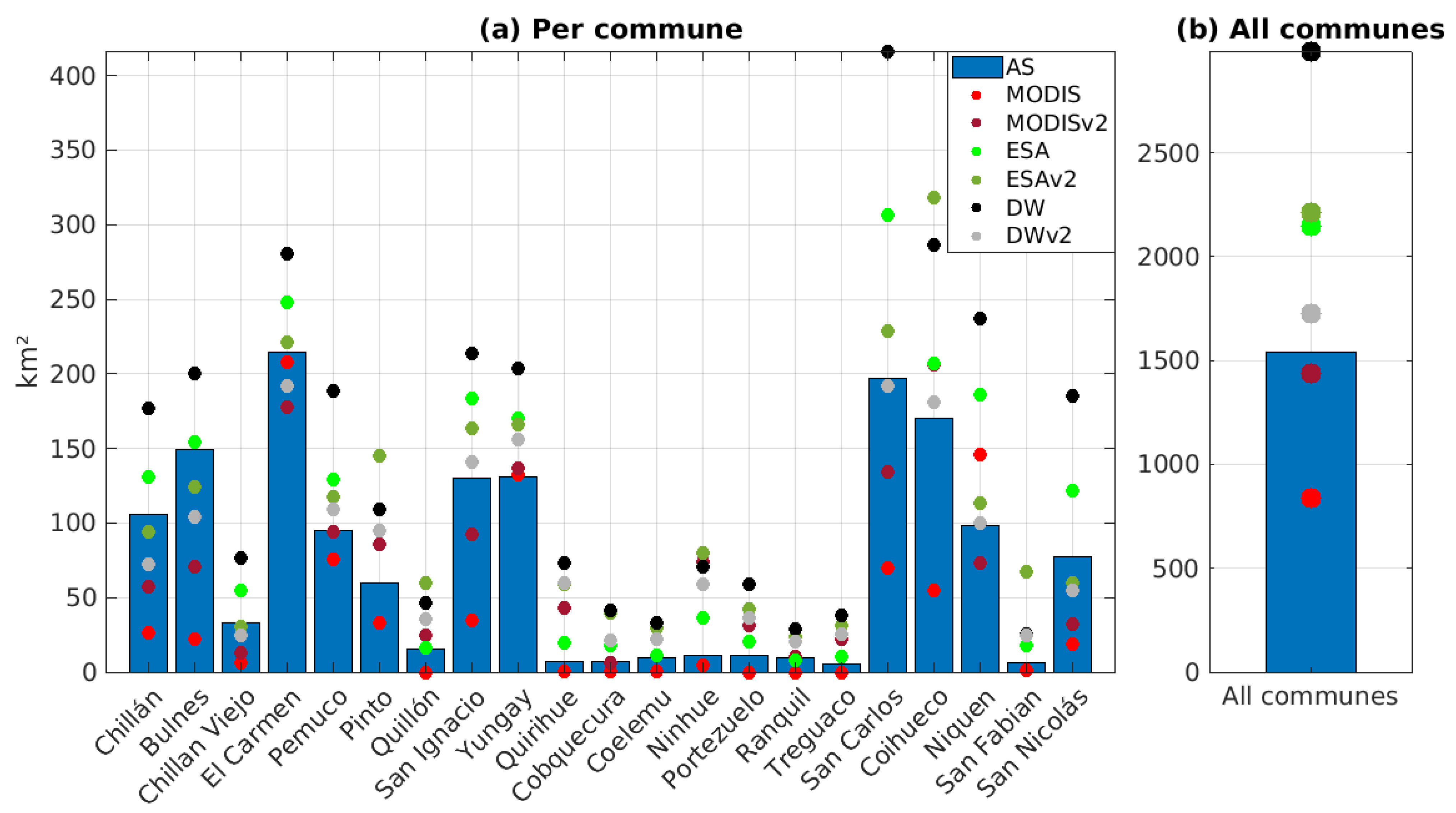
| Chillán (473.69) | 29.72 | 4.94 | 192.23 | 105.89 | 26.44 | 57.05 | 130.99 | 93.93 | 177.09 | 72.02 | 270.84 |
| Bulnes (425.09) | 36.84 | 7.19 | 227.15 | 149.18 | 22.47 | 70.83 | 154.39 | 123.84 | 200.41 | 104.18 | 281.18 |
| Chillán Viejo (262.80) | 12.92 | 2.20 | 65.97 | 32.75 | 6.20 | 12.77 | 54.99 | 30.12 | 76.83 | 24.53 | 86.73 |
| El Carmen (667.39) | 87.83 | 133.72 | 173.23 | 214.63 | 207.54 | 178.05 | 247.75 | 220.97 | 280.18 | 192.04 | 334.21 |
| Pemuco (561.52) | 68.24 | 72.24 | 103.69 | 94.88 | 75.73 | 93.97 | 129.20 | 117.90 | 188.22 | 109.29 | 181.57 |
| Pinto (1099.70) | 28.09 | 5.78 | 129.67 | 59.93 | 33.14 | 86.08 | 94.54 | 145.47 | 109.26 | 95.27 | 139.49 |
| Quillón (405.44) | 3.41 | 0 | 110.17 | 15.53 | 0 | 24.40 | 16.56 | 59.91 | 46.35 | 35.35 | 121.00 |
| San Ignacio (363.48) | 88.87 | 11.78 | 174.09 | 130.19 | 35.05 | 92.16 | 183.49 | 163.16 | 213.91 | 141.07 | 261.56 |
| Yungay (824.40) | 78.10 | 125.06 | 146.59 | 130.69 | 132.65 | 136.98 | 170.52 | 165.63 | 203.80 | 156.02 | 231.53 |
| Quirihue (591.07) | 8.95 | 0 | 87.03 | 7.09 | 0.60 | 42.90 | 20.07 | 58.55 | 73.41 | 59.38 | 89.89 |
| Cobquecura (570.05) | 15.12 | 0 | 38.65 | 7.09 | 0.60 | 6.12 | 18.05 | 39.35 | 41.37 | 21.73 | 64.01 |
| Coelemu (341.66) | 4.50 | 0 | 47.84 | 9.76 | 0.20 | 29.37 | 11.40 | 29.37 | 33.04 | 22.19 | 57.83 |
| Ninhue (402.63) | 11.07 | 2.28 | 101.16 | 10.93 | 4.90 | 73.74 | 36.75 | 79.64 | 70.41 | 58.92 | 104.94 |
| Portezuelo (290.03) | 5.01 | 0 | 67.08 | 11.25 | 0 | 31.10 | 20.88 | 42.16 | 59.30 | 36.50 | 92.72 |
| Ránquil (247.57) | 1.06 | 0 | 51.28 | 9.78 | 0 | 10.53 | 8.19 | 23.95 | 29.14 | 20.40 | 57.46 |
| Treguaco (315.22) | 7.42 | 0 | 46.68 | 5.28 | 0 | 21.77 | 10.63 | 31.23 | 37.69 | 25.83 | 81.32 |
| San Carlos (873.53) | 108.99 | 16.72 | 417.43 | 196.58 | 69.92 | 134.31 | 306.15 | 228.83 | 416.46 | 191.82 | 599.61 |
| Coihueco (1773.29) | 90.16 | 24.13 | 304.12 | 170.01 | 54.52 | 206.33 | 206.73 | 318.07 | 286.23 | 181.38 | 341.98 |
| Ñiquen (492.22) | 65.70 | 100.25 | 205.12 | 98.05 | 146.00 | 73.02 | 186.06 | 113.72 | 236.89 | 99.77 | 327.87 |
| San Fabián (1540.85) | 4.53 | 0 | 74.16 | 6.14 | 1.20 | 25.38 | 17.79 | 67.13 | 25.14 | 24.75 | 39.16 |
| San Nicolás (567.59) | 24.22 | 4.54 | 189.59 | 77.49 | 18.72 | 32.28 | 121.94 | 59.76 | 185.13 | 55.15 | 237.98 |
Appendix C


References
- Zambrano, F.; Vrieling, A.; Nelson, A.; Meroni, M.; Tadesse, T. Prediction of drought-induced reduction of agricultural productivity in Chile from MODIS, rainfall estimates, and climate oscillation indices. Remote Sens. Environ. 2018, 219, 15–30. [Google Scholar] [CrossRef]
- Zúñiga, F.; Jaime, M.; Salazar, C. Crop farming adaptation to droughts in small-scale dryland agriculture in Chile. Water Resour. Econ. 2021, 34, 100176. [Google Scholar] [CrossRef]
- Instituto Nacional de Estadísticas. Available online: https://www.ine.gob.cl/ (accessed on 6 May 2024).
- Nguyen, L.H.; Joshi, D.R.; Clay, D.E.; Henebry, G.M. Characterizing land cover/land use from multiple years of Landsat and MODIS time series: A novel approach using land surface phenology modeling and random forest classifier. Remote Sens. Environ. 2020, 238, 111017. [Google Scholar] [CrossRef]
- Regasa, M.S.; Nones, M.; Adeba, D. A review on land use and land cover change in Ethiopian basins. Land 2021, 10, 585. [Google Scholar] [CrossRef]
- Ustaoglu, E.; Aydınoglu, A.C. Regional variations of land-use development and land-use/cover change dynamics: A case study of Turkey. Remote Sens. 2019, 11, 885. [Google Scholar] [CrossRef]
- Brown, C.F.; Brumby, S.P.; Guzder-Williams, B.; Birch, T.; Hyde, S.B.; Mazzariello, J.; Czerwinski, W.; Pasquarella, V.; Haertel, R.; Ilyushchenko, S.; et al. Dynamic World, Near real-time global 10 m land use land cover mapping. Sci. Data 2022, 9, 251. [Google Scholar] [CrossRef]
- Dong, R.; Li, C.; Fu, H.; Wang, J.; Li, W.; Yao, Y.; Gan, L.; Yu, L.; Gong, P. Improving 3-m resolution land cover mapping through efficient learning from an imperfect 10-m resolution map. Remote Sens. 2020, 12, 1418. [Google Scholar] [CrossRef]
- Petrişor, A.I.; Sirodoev, I.; Ianoş, I. Trends in the national and regional transitional dynamics of land cover and use changes in Romania. Remote Sens. 2020, 12, 230. [Google Scholar] [CrossRef]
- Friedl, M.A.; Woodcock, C.E.; Olofsson, P.; Zhu, Z.; Loveland, T.; Stanimirova, R.; Arevalo, P.; Bullock, E.; Hu, K.-T.; Zhang, Y.; et al. Medium spatial resolution mapping of global land cover and land cover change across multiple decades from Landsat. Front. Remote Sens. 2020, 3, 894571. [Google Scholar] [CrossRef]
- Plummer, S.; Lecomte, P.; Doherty, M. The ESA Climate Change Initiative (CCI): A European contribution to the generation of the Global Climate Observing System. Remote Sens. Environ. 2017, 203, 2–8. [Google Scholar] [CrossRef]
- Sulla-Menashe, D.; Gray, J.M.; Abercrombie, S.P.; Friedl, M.A. Hierarchical mapping of annual global land cover 2001 to present: The MODIS Collection 6 Land Cover product. Remote Sens. Environ. 2019, 222, 183–194. [Google Scholar] [CrossRef]
- Zhao, T.; Zhang, X.; Gao, Y.; Mi, J.; Liu, W.; Wang, J.; Jiang, M.; Liu, L. Assessing the accuracy and consistency of six fine-resolution global land cover products using a novel stratified random sampling validation dataset. Remote Sens. 2023, 15, 2285. [Google Scholar] [CrossRef]
- Graesser, J.; Ramankutty, N. Detection of cropland field parcels from Landsat imagery. Remote Sens. Environ. 2017, 201, 165–180. [Google Scholar] [CrossRef]
- Phan, D.C.; Trung, T.H.; Truong, V.T.; Sasagawa, T.; Vu, T.P.T.; Bui, D.T.; Hayashi, M.; Tadono, T.; Nasahara, K.N. First comprehensive quantification of annual land use/cover from 1990 to 2020 across mainland Vietnam. Sci. Rep. 2021, 11, 9979. [Google Scholar] [CrossRef]
- Gorelick, N.; Hancher, M.; Dixon, M.; Ilyushchenko, S.; Thau, D.; Moore, R. Google Earth Engine: Análisis geoespacial a escala planetaria para todos. Teledetección Del Medio Ambiente 2017, 202, 18–27. [Google Scholar]
- Volke, M.; Abarca-Del-Rio, R.; Warner, T.A. Cost-effective disaster-induced land cover analysis: A semi-automatic methodology Using machine learning and satellite imagery. Int. J. Remote Sens. 2024, 45, 279–305. [Google Scholar] [CrossRef]
- Venter, Z.S.; Barton, D.N.; Chakraborty, T.; Simensen, T.; Singh, G. Global 10 m land use land cover datasets: A comparison of dynamic world, world cover and esri land cover. Remote Sens. 2022, 14, 4101. [Google Scholar] [CrossRef]
- Bagan, H.; Millington, A.; Takeuchi, W.; Yamagata, Y. Spatiotemporal analysis of deforestation in the Chapare region of Bolivia using LANDSAT images. Land Degrad. Dev. 2020, 31, 3024–3039. [Google Scholar] [CrossRef]
- Zhang, H.K.; Roy, D.P. Using the 500 m MODIS land cover product to derive a consistent continental scale 30 m Landsat land cover classification. Remote Sens. Environ. 2017, 197, 15–34. [Google Scholar] [CrossRef]
- Huang, H.; Wang, J.; Liu, C.; Liang, L.; Li, C.; Gong, P. The migration of training samples towards dynamic global land cover mapping. ISPRS J. Photogramm. Remote Sens. 2020, 161, 27–36. [Google Scholar] [CrossRef]
- Teluguntla, P.; Thenkabail, P.; Oliphant, A.; Xiong, J.; Gumma, M.K.; Congalton, R.G.; Yadav, K.; Huete, A. A 30-m landsat-derived cropland extent product of Australia and China using random forest machine learning algorithm on Google Earth Engine cloud computing platform. ISPRS J. Photogramm. Remote Sens. 2018, 144, 325–340. [Google Scholar] [CrossRef]
- Phalke, A.R.; Özdoğan, M.; Thenkabail, P.S.; Erickson, T.; Gorelick, N.; Yadav, K.; Congalton, R.G. Mapping croplands of Europe, Middle East, Russia, and Central Asia using Landsat, Random Forest, and Google Earth Engine. ISPRS J. Photogramm. Remote Sens. 2020, 167, 104–122. [Google Scholar] [CrossRef]
- Radoux, J.; Lamarche, C.; Van Bogaert, E.; Bontemps, S.; Brockmann, C.; Defourny, P. Automated Training Sample Extraction for Global Land Cover Mapping. Remote Sens. 2014, 6, 3965–3987. [Google Scholar] [CrossRef]
- Roy, D.P.; Kumar, S.S. Multi-year MODIS active fire type classification over the Brazilian Tropical Moist Forest Biome. Int. J. Digit. Earth 2017, 10, 54–84. [Google Scholar] [CrossRef]
- Zhang, X.; Liu, L.; Chen, X.; Gao, Y.; Xie, S.; Mi, J. GLC_FCS30: Global land-cover product with fine classification system at 30 m using time-series Landsat imagery. Earth Syst. Sci. Data 2021, 13, 2753–2776. [Google Scholar] [CrossRef]
- Zanaga, D.; Van De Kerchove, R.; Daems, D.; De Keersmaecker, W.; Brockmann, C.; Kirches, G.; Wevers, J.; Cartus, O.; Santoro, M.; Fritz, S.; et al. ESA WorldCover 10 m 2021 v200. 2022. Available online: https://zenodo.org/records/7254221 (accessed on 15 May 2024).
- USGS: Landsat Missions. Available online: https://www.usgs.gov/landsat-missions (accessed on 9 May 2024).
- Copernicus Data Space Ecosystem (CDSE): Sentinel-2. Available online: https://dataspace.copernicus.eu/explore-data/data-collections/sentinel-data/sentinel-2 (accessed on 9 May 2024).
- Earth Engine Data Catalog (EEDC). Available online: https://developers.google.com/earth-engine/datasets (accessed on 9 May 2024).
- Valderrama, N.; Azocar, G.; Juarez, F. Agricultura y productividad: Tendencias y determinantes en una región de Chile central (Determining Factors and Trends of Agricultural Productivity in a Region of Central Chile). RAN-Rev. Acad. Neg. 2019, 5. [Google Scholar]
- ODEPA: Región de Ñuble Información Regional 2019. Available online: https://www.odepa.gob.cl/wp-content/uploads/2018/11/%C3%91uble.pdf (accessed on 24 May 2024).
- National Statistics Institute (INE). Available online: https://www.ine.gob.cl/censoagropecuario (accessed on 9 May 2024).
- Tucker, C.J. Red and photographic infrared linear combinations for monitoring vegetation. Remote Sens. Environ. 1979, 8, 127–150. [Google Scholar] [CrossRef]
- Xu, H. Modification of normalised difference water index (NDWI) to enhance open water features in remotely sensed imagery. Int. J. Remote Sens. 2006, 27, 3025–3033. [Google Scholar] [CrossRef]
- Huete, A.R.; Didan, K.; van Leeuwen, W.J.D.; Vermote, E.F. Global-scale analysis of vegetation indices for moderate resolution monitoring of terrestrial vegetation. Remote Sens. Earth Sci. Ocean Sea Ice Appl. 1999, 3868, 141–151. [Google Scholar]
- Miller, J.D.; Thode, A.E. Quantifying burn severity in a heterogeneous landscape with a relative version of the delta Normalized Burn Ratio (dNBR). Remote Sens. Environ. 2007, 109, 66–80. [Google Scholar] [CrossRef]
- Wang, Q.; Blackburn, G.A.; Onojeghuo, A.O.; Dash, J.; Zhou, L.; Zhang, Y.; Atkinson, P.M. Fusion of Landsat 8 OLI and Sentinel-2 MSI Data. IEEE Trans. Geosci. Remote Sens. 2017, 55, 3885–3899. [Google Scholar] [CrossRef]
- Zhu, Z.; Wang, S.; Woodcock, C.E. Improvement and expansion of the Fmask algorithm: Cloud, cloud shadow, and snow detection for Landsats 4–7, 8, and Sentinel 2 images. Remote Sens. Environ. 2015, 159, 269–277. [Google Scholar] [CrossRef]
- Yang, J.; Yu, L.; Mallinis, G.; Orusa, T.; Cammareri, D.; Mondino, E.B. A Possible Land Cover EAGLE Approach to Overcome Remote Sensing Limitations in the Alps Based on Sentinel-1 and Sentinel-2: The Case of Aosta Valley (NW Italy). Remote Sens. 2023, 15, 178. [Google Scholar]
- Wang, X.; Zhang, Y.; Zhang, K.; Wang, X.; Zhang, Y.; Zhang, K. Automatic 10 m Forest Cover Mapping in 2020 at China’s Han River Basin by Fusing ESA Sentinel-1/Sentinel-2 Land Cover and Sentinel-2 near Real-Time Forest Cover Possibility. Forests 2023, 14, 1133. [Google Scholar] [CrossRef]
- Venkatappa, M.; Sasaki, N.; Shrestha, R.P.; Tripathi, N.K.; Ma, H.O. Determination of Vegetation Thresholds for Assessing Land Use and Land Use Changes in Cambodia using the Google Earth Engine Cloud-Computing Platform. Remote Sens. 2019, 11, 1514. [Google Scholar] [CrossRef]
- Ghorbanian, A.; Kakooei, M.; Amani, M.; Mahdavi, S.; Mohammadzadeh, A.; Hasanlou, M. Improved land cover map of Iran using Sentinel imagery within Google Earth Engine and a novel automatic workflow for land cover classification using migrated training samples. ISPRS J. Photogramm. Remote Sens. 2020, 167, 276–288. [Google Scholar] [CrossRef]
- Olofsson, P.; Foody, G.M.; Herold, M.; Stehman, S.V.; Woodcock, C.E.; Wulder, M.A. Good practices for estimating area and assessing accuracy of land change. Remote Sens. Environ. 2014, 148, 42–57. [Google Scholar] [CrossRef]
- Breiman, L. Random forests. Mach. Learn. 2001, 45, 5–32. [Google Scholar] [CrossRef]
- He, Y.; Lee, E.; Warner, T.A. A time series of annual land use and land cover maps of China from 1982 to 2013 generated using AVHRR GIMMS NDVI3g data. Remote Sens. Environ. 2017, 199, 201–217. [Google Scholar] [CrossRef]
- Naidoo, L.; Cho, M.A.; Mathieu, R.; Asner, G. Classification of savanna tree species, in the Greater Kruger National Park region, by integrating hyperspectral and LiDAR data in a Random Forest data mining environment. ISPRS J. Photogramm. Remote Sens. 2012, 69, 167–179. [Google Scholar] [CrossRef]
- Rodriguez-Galiano, V.F.; Ghimire, B.; Rogan, J.; Chica-Olmo, M.; Rigol-Sanchez, J.P. An assessment of the effectiveness of a random forest classifier for land-cover classification. ISPRS J. Photogramm. Remote Sens. 2012, 67, 93–104. [Google Scholar] [CrossRef]
- Belgiu, M.; Drăguţ, L. Random forest in remote sensing: A review of applications and future directions. ISPRS J. Photogramm. Remote Sens. 2016, 114, 24–31. [Google Scholar] [CrossRef]
- Pelletier, C.; Valero, S.; Inglada, J.; Champion, N.; Dedieu, G. Assessing the robustness of Random Forests to map land cover with high resolution satellite image time series over large areas. Remote Sens. Environ. 2016, 187, 156–168. [Google Scholar] [CrossRef]
- Shiferaw, H.; Bewket, W.; Eckert, S. Performances of machine learning algorithms for mapping fractional cover of an invasive plant species in a dryland ecosystem. Ecol. Evol. 2019, 9, 2562–2574. [Google Scholar] [CrossRef]
- Prudente, V.H.R.; Martins, V.S.; Vieira, D.C.; e Silva, N.R.D.F.; Adami, M.; Sanches, I.D.A. Limitations of cloud cover for optical remote sensing of agricultural areas across South America. Remote Sens. Appl. Soc. Environ. 2020, 20, 100414. [Google Scholar] [CrossRef]
- Heck, E.; de Beurs, K.M.; Owsley, B.C.; Henebry, G.M. Evaluation of the MODIS collections 5 and 6 for change analysis of vegetation and land surface temperature dynamics in North and South America. ISPRS J. Photogramm. Remote Sens. 2019, 156, 121–134. [Google Scholar] [CrossRef]
- IDE Minagri: Catastro de Uso de Suelo y Vegetación (CONAF). Available online: https://ide.minagri.gob.cl/geoweb/2019/11/22/planificacion-catastral/ (accessed on 9 May 2024).
- Inglada, J.; Vincent, A.; Arias, M.; Tardy, B.; Morin, D.; Rodes, I. Operational High Resolution Land Cover Map Production at the Country Scale Using Satellite Image Time Series. Remote Sens. 2017, 9, 95. [Google Scholar] [CrossRef]
- Wessels, K.J.; van den Bergh, F.; Roy, D.P.; Salmon, B.P.; Steenkamp, K.C.; MacAlister, B.; Swanepoel, D.; Jewitt, D. Rapid Land Cover Map Updates Using Change Detection and Robust Random Forest Classifiers. Remote Sens. 2016, 8, 888. [Google Scholar] [CrossRef]

| Categories | 2020–2021 | |
|---|---|---|
| Original classes | Total Cereals Tubers Industrial crops Vegetables fruit trees Vines Flowers Seedbeds Plant nurseries Fodder Improved-grasslands * | |
| Grouped classes | Irrigation, dry, total | |
| Covered area | Ñuble region | Chillán, Bulnes, Chillán Viejo, El Carmen, Pemuco, Pinto, Quillón, San Ignacio, Yungay, Quirihue, Cobquecura, Coelemu. Ninhue, Portezuelo, Ránquil, Treguaco, San Carlos, Coihueco, Ñiquén, San Fabián y San Nicolás. |
| Database | Available Period | Used Period | Spatial Resol. [m] | Classes or Variables | Selected Classes for Agriculture |
|---|---|---|---|---|---|
| ESA WorldCover 10 m v200 [27] | 2021 | 10 | Tree cover, shrubland, grassland, cropland, built-up, bare/sparse vegetation, snow and ice, permanent water bodies, herbaceous wetland, mangroves, moss and lichen | Cropland: Land covered with annual crops that are sown/planted and harvestable at least once within the 12 months after the sowing/planting date. The annual cropland produces an herbaceous cover and is sometimes combined with trees or woody vegetation. Note that perennial woody crops are classified as the appropriate tree cover or shrub land cover type. Greenhouses are considered built-up. | |
| Dynamic World V1 [7] | 27 June 2015–present (revisit time: 2–5 days depending on latitude) | 8/2020–3/2021 | 10 | Water, trees, grass, flooded vegetation, crops, shrub and scrub, built, bare, snow and ice | Crops: Human-planted/plotted cereals, grasses and crops. |
| MCD12Q1.061 MODIS Land Cover Type Yearly Global 500 m [12,30] | 2001–2022 (yearly) | 2021 | 500 | Several types of forest: evergreen needleleaf, evergreen broadleaf, deciduous needleleaf, deciduous broadleaf, and mixed, closed shrublands, open shrublands, woody savannas, savannas, grasslands, permanent wetlands, croplands, urban and built-up lands, cropland/natural vegetation mosaics, permanent snow and ice, barren and water bodies. | Cropland: Areas where at least 60% is cultivated cropland. Cropland/natural vegetation mosaics: Mosaics of small-scale cultivation (40–60%) with natural trees, shrubs or herbaceous vegetation. |
| Landsat 8 Surface Reflectance | February 2013–present (16-day revisit time) | August 2020 –March 2021 | 30 | NDVI (normalized difference vegetation index) [34], NDWI (normalized difference water index) [35], EVI (enhanced vegetation index) [36] and NBR (normalized burn rate) [37] | - |
| Sentinel-2 Surface Reflectance | March 2017–present (10-day revisit time) | 10 | |||
| Commune | MODIS | MODIS v2 | ESA | ESA v2 | DW | DW v2 |
|---|---|---|---|---|---|---|
| Chillán | −75 | −46 | 24 | −11 | 67 | −32 |
| Bulnes | −85 | −53 | 3 | −17 | 34 | −30 |
| Chillán Viejo | −81 | −61 | 68 | −8 | 135 | −25 |
| El Carmen | −3 | −17 | 15 | 3 | 31 | −11 |
| Pemuco | −20 | −1 | 36 | 24 | 98 | 15 |
| Pinto | −45 | 43 | 58 | 143 | 82 | 59 |
| Quillón | −100 | 57 | 7 | 286 | 198 | 128 |
| San Ignacio | −73 | −29 | 41 | 25 | 64 | 8 |
| Yungay | 2 | 5 | 30 | 27 | 56 | 19 |
| Quirihue | −92 | 505 | 83 | 726 | 935 | 738 |
| Cobquecura | −92 | −14 | 155 | 455 | 483 | 206 |
| Coelemu | −98 | 201 | 17 | 201 | 239 | 127 |
| Ninhue | −55 | 575 | 236 | 629 | 544 | 439 |
| Portezuelo | −100 | 176 | 86 | 275 | 427 | 224 |
| Ránquil | −100 | 8 | −16 | 145 | 198 | 109 |
| Treguaco | −100 | 312 | 101 | 491 | 614 | 389 |
| San Carlos | −64 | −32 | 56 | 16 | 112 | −2 |
| Coihueco | −68 | 21 | 22 | 87 | 68 | 7 |
| Ñiquen | 49 | −26 | 90 | 16 | 142 | 2 |
| San Fabián | −80 | 313 | 190 | 993 | 309 | 303 |
| San Nicolás | −76 | −58 | 57 | −23 | 139 | −29 |
| MODIS | Tr | Cr | Ur | Gr | Sh | Ba | UA | ||
| Tr | 238 | 4 | 8 | 7 | 1 | 42 | 0.77 | ||
| Cr | 21 | 1156 | 266 | 5 | 0 | 52 | 0.92 | ||
| Ur | 0 | 53 | 231 | 2 | 0 | 14 | 0.40 | ||
| Gr | 5 | 10 | 16 | 168 | 45 | 56 | 0.62 | ||
| Sh | 0 | 0 | 0 | 33 | 265 | 0 | 0.84 | ||
| Ba | 47 | 36 | 51 | 56 | 4 | 106 | 0.39 | ||
| PA | 0.79 | 0.77 | 0.77 | 0.56 | 0.89 | 0.35 | OA | 0.72 | |
| ESA | Tr | Cr | Ur | Gr | Sh | Ba | UA | ||
| Tr | 289 | 1 | 8 | 1 | 0 | 0 | 0.95 | ||
| Cr | 14 | 1161 | 268 | 56 | 1 | 0 | 0.99 | ||
| Ur | 0 | 4 | 251 | 17 | 28 | 0 | 0.44 | ||
| Gr | 1 | 4 | 21 | 268 | 6 | 0 | 0.77 | ||
| Sh | 0 | 0 | 19 | 2 | 272 | 7 | 0.84 | ||
| Ba | 0 | 0 | 0 | 2 | 17 | 279 | 0.98 | ||
| PA | 0.97 | 0.77 | 0.84 | 0.89 | 0.91 | 0.94 | OA | 0.85 | |
| DW | Tr | Cr | Ur | Gr | Sh | Ba | UA | ||
| Tr | 281 | 2 | 0 | 1 | 15 | 0 | 0.88 | ||
| Cr | 16 | 1390 | 36 | 4 | 54 | 0 | 0.96 | ||
| Ur | 0 | 2 | 291 | 5 | 2 | 0 | 0.82 | ||
| Gr | 4 | 42 | 19 | 195 | 39 | 0 | 0.76 | ||
| Sh | 17 | 5 | 8 | 2 | 266 | 0 | 0.71 | ||
| Ba | 0 | 0 | 2 | 50 | 0 | 244 | 1.00 | ||
| PA | 0.94 | 0.93 | 0.97 | 0.65 | 0.89 | 0.82 | OA | 0.89 |
Disclaimer/Publisher’s Note: The statements, opinions and data contained in all publications are solely those of the individual author(s) and contributor(s) and not of MDPI and/or the editor(s). MDPI and/or the editor(s) disclaim responsibility for any injury to people or property resulting from any ideas, methods, instructions or products referred to in the content. |
© 2024 by the authors. Licensee MDPI, Basel, Switzerland. This article is an open access article distributed under the terms and conditions of the Creative Commons Attribution (CC BY) license (https://creativecommons.org/licenses/by/4.0/).
Share and Cite
Volke, M.; Pedreros-Guarda, M.; Escalona, K.; Acuña, E.; Orrego, R. Assessment of Semi-Automated Techniques for Crop Mapping in Chile Based on Global Land Cover Satellite Data. Remote Sens. 2024, 16, 2964. https://doi.org/10.3390/rs16162964
Volke M, Pedreros-Guarda M, Escalona K, Acuña E, Orrego R. Assessment of Semi-Automated Techniques for Crop Mapping in Chile Based on Global Land Cover Satellite Data. Remote Sensing. 2024; 16(16):2964. https://doi.org/10.3390/rs16162964
Chicago/Turabian StyleVolke, Matías, María Pedreros-Guarda, Karen Escalona, Eduardo Acuña, and Raúl Orrego. 2024. "Assessment of Semi-Automated Techniques for Crop Mapping in Chile Based on Global Land Cover Satellite Data" Remote Sensing 16, no. 16: 2964. https://doi.org/10.3390/rs16162964
APA StyleVolke, M., Pedreros-Guarda, M., Escalona, K., Acuña, E., & Orrego, R. (2024). Assessment of Semi-Automated Techniques for Crop Mapping in Chile Based on Global Land Cover Satellite Data. Remote Sensing, 16(16), 2964. https://doi.org/10.3390/rs16162964