Crop Water Status Analysis from Complex Agricultural Data Using UMAP-Based Local Biplot

Abstract

To optimize growth and management, precision agriculture relies on a deep understanding of agricultural dynamics, particularly crop water status analysis. Leveraging unmanned aerial vehicles, we can efficiently acquire high-resolution spatiotemporal samples by utilizing remote sensors. However, non-linear relationships among data features, localized within specific subgroups, frequently emerge in agricultural data. Interpreting these complex patterns requires sophisticated analysis due to the presence of noise, high variability, and non-stationarity behavior in the collected samples. Here, we introduce Local Biplot, a methodological framework tailored for discerning meaningful data patterns in non-stationary contexts for precision agriculture. Local Biplot relies on the well-known uniform manifold approximation and projection method, such as UMAP, and local affine transformations to codify non-stationary and non-linear data patterns while maintaining interpretability. This lets us find important clusters for transformation and projection within a single global axis pair. Hence, our framework encompasses variable and observational contributions within individual clusters. At the same time, we provide a relevance analysis strategy to help explain why those clusters exist, facilitating the understanding of data dynamics while favoring interpretability. We demonstrated our method’s capabilities through experiments on both synthetic and real-world datasets, covering scenarios involving grass and rice crops. Moreover, we use random forest and linear regression models to predict water status variables from our Local Biplot-based feature ranking and clusters. Our findings revealed enhanced clustering and prediction capability while emphasizing the importance of input features in precision agriculture. As a result, Local Biplot is a useful tool to visualize, analyze, and compare the intricate underlying patterns and internal structures of complex agricultural datasets.

1. Introduction

The accurate assessment of crop water status, which refers to the level of hydration within a plant, is critical in precision agriculture (PA) for water-intensive crops. Furthermore, climate change necessitates optimizing water usage to meet increased drought threats [1,2]. By monitoring crop water status indicators, such as soil moisture and plant stress, and understanding crop responses, we can tailor irrigation practices [3,4]. When it comes to PA, understanding how temporal or conditional variations in different factors can significantly impact crop growth, productivity, and overall agricultural management is essential [5]. Still, dynamic changes in soil moisture due to spatial and temporal variability, life cycle patterns, plant water uptake, environmental aspects, and irrigation practices can exhibit non-stationary behaviors, meaning they do not follow a fixed distribution or consistent patterns over space and time. For example, in rice crops, temperature fluctuations, soil moisture levels, and day length can dynamically influence flowering time and other plant properties [6]. Thus, addressing non-linear and non-stationary patterns in agricultural data analysis is essential for accurately assessing water status, improving decision-making, and effective agricultural management [7,8].

Conventional methods like soil moisture sensors, leaf-level measurements, laboratory analysis, and manual field surveys are often time-consuming and labor-intensive. Recent developments in unmanned aerial vehicle (UAV)-based remote sensing (RS) techniques make data collection for crop characterization and monitoring more efficient, as they are non-invasive, non-destructive, accurate, and cost-effective [9]. By combining the different wavelengths of light that plants reflect and absorb, vegetation indices (VIs) provide valuable insights, such as canopy biomass and chlorophyll content [10]. Nonetheless, effectively extracting useful information from the large volumes of samples generated by integrating field data with high-resolution remote and proximal sensors can be cumbersome [11]. Additionally, noise, data source conflicts, and spatiotemporal UAV disparities caused by weather changes and sub-optimal sampling further complicate the training of accurate and reliable models [12,13].

As agricultural research evolves, different techniques have emerged to conveniently explore and organize data to extract valuable knowledge [14]. These approaches include descriptive and exploratory analysis [15,16], clustering [17], multivariate analysis for exploring inter-variable relationships [18], time series analysis for studying temporal patterns [19], and predictive modeling [20,21]. Visual representations, such as biplots [22,23], are typically the preferred method for achieving a 2D plot that is immediate, direct, and simple to comprehend for both input feature and sample relationships in a low-dimensional space. The latter assists in the identification of critical variables, resulting in the completion of duties such as cluster visualization, correlation highlighting, and feature selection. While traditional biplots remain fundamental, advanced statistical tools have emerged to address some of their limitations, focusing on genotype-by-environment interactions to highlight superior crop varieties. Thus, their suitability depends on the specific research question and data characteristics [16,24]. Additionally, traditional statistical methods face significant challenges when dealing with the complexities inherent in high-dimensional agricultural datasets [25]. One of the primary constraints is their inability to accurately represent the true dynamics of agricultural processes due to their difficulty with non-linear relationships. Then, the variables frequently interact in complex and non-linear ways, resulting in oversimplified models [26].

Here, we introduce the Local Biplot methodological framework, which uses 2D data visualization and input feature ranking within localized clusters to identify meaningful patterns, with a specific focus on water status analysis in multi-temporal agricultural data. Our Local Biplot employs a uniform manifold approximation and projection (UMAP)-based algorithm to embed the input data within a 2D feature space dealing with nonlinear and non-stationary agricultural data dynamics [27]. Then, the well-known K-means algorithm is used to cluster the samples from the UMAP 2D space. Further, to provide a complete picture of the local relationships between the variables and samples, a local affine transformation is then applied to map the input feature variability-based rankings to the 2D low-dimensional space. Hence, this framework encompasses variable/observation contributions within individual clusters in the same figure, facilitating the understanding of data dynamics to overcome pressing agricultural challenges such as climate variability, unsustainable agricultural practices, and inefficient use of water resources. Local Biplot is tested on both synthetic and real-world datasets. In particular, forage grasses and rice crops are tested to highlight relevant agricultural patterns related to water status studies in PA. Moreover, to investigate the influence of non-stationary data dynamics and inter-cluster relationships in the assessment of water content-related variables, we conducted experiments using random forest (RF) and linear regression (LR) models to estimate crop water status variables, such as the breeding score for grass and canopy water content (CWC) for rice.

The agenda for this paper is as follows: Section 2 describes the materials and methods. Section 3 present the experiments and results and Section 4 discuss the results obtained. Finally, Section 5 outlines the conclusions and future work.

2. Materials and Methods

2.1. Biplot Fundamentals

Let $\mathbf{X}\in {\mathbb{R}}^{N\times P}$ be an input matrix with centered and standardized P-dimensional features and N samples represented by row vectors ${\mathbf{x}}_n\in {\mathbb{R}}^P$. Thus, $\mathbf{X}$ can be decomposed as $\mathbf{X}=\mathbf{U}\mathbf{S}{\mathbf{V}}^{\top }$, where $\mathbf{U}\in {\mathbb{R}}^{N\times M}$ and $\mathbf{V}\in {\mathbb{R}}^{P\times M}$ are orthonormal matrices, and $\mathbf{S}\in {\mathbb{R}}^{M\times M}$ is diagonal with non-negative elements. This singular value decomposition (SVD) allows for a low-dimensional representation $\tilde{\mathbf{X}}={\mathbf{U}}_M{\mathbf{S}}_M{\mathbf{V}}_M^{\top }$, optimizing:

$${\tilde{\mathbf{X}}}^{*}=arg\underset{\tilde{\mathbf{X}}}{min}{\parallel \mathbf{X}-\tilde{\mathbf{X}}\parallel }_{\mathrm{F}}^2.$$

(1)

Of note, the eigenvectors for the M highest singular values in $\mathbf{S}$ are held by ${\mathbf{U}}_M$ and ${\mathbf{V}}_M$. In biplot analysis, ${\mathbf{U}}_M{\mathbf{S}}_M^{0.5}$ and ${\mathbf{S}}_M^{0.5}{\mathbf{V}}_M^{\top }$, with $M=2$, are constructed to visualize relationships between samples and features, respectively. These matrices project data onto a 2D space, highlighting input data clusters and feature linear dependencies.

2.2. Uniform Manifold Approximation and Projection (UMAP)

Given the high-dimensional matrix $\mathbf{X}$ and the Euclidean distance function $\mathrm{d}(·,·)\in {\mathbb{R}}^{+}$, UMAP aims to find a low-dimensional embedding $\mathbf{Z}\in {\mathbb{R}}^{N\times M}$ that preserves both global and local neighborhoods from $\mathbf{X}$, promoting the main non-linear data relationships. Then, a K-nearest neighbor (KNN)-based graph is built based on a local metric, yielding:

$${\theta }_n=\underset{n^{\prime }\in K}{min}\mathrm{d}({\mathbf{x}}_n,{\mathbf{x}}_{n^{\prime }}),$$

(2)

where ${\theta }_n\in {\mathbb{R}}^{+}$ holds the minimum distance within the n-th neighborhood with K neighbors ${\mathbf{x}}_{n^{\prime }}$ centered on ${\mathbf{x}}_n.$ A localized entropy value ${\sigma }_n\in {\mathbb{R}}^{+}$ is computed by solving:

$$\sum _{n^{\prime }=1}^{K}exp\left(-{\displaystyle \frac{\mathrm{d}({\mathbf{x}}_n,{\mathbf{x}}_{n^{\prime }})-{\theta }_n}{{\sigma }_n}}\right)=log\left(K\right).$$

(3)

Afterward, UMAP constructs a fuzzy simplicial complex, representing the high-dimensional graph $\mathcal{G}=(\mathbf{X},\mathbf{W})$, where edges are defined by local connectivity through the weights in $\mathbf{W}\in {[0,1]}^{N\times N}$:

$$w_{n{n}^{\prime }}=exp\left(-max\left(0,{\displaystyle \frac{\mathrm{d}({\mathbf{x}}_n,{\mathbf{x}}_{n^{\prime }})-{\theta }_n}{{\sigma }_n}}\right)\right).$$

(4)

Likewise, a low-dimensional weight matrix $\tilde{\mathbf{W}}\in {[0,1]}^{N\times N}$ is computed as:

$${\tilde{w}}_{n{n}^{\prime }}={\left(1+\alpha \mathrm{d}{({\mathbf{z}}_n,{\mathbf{z}}_{n^{\prime }})}^2\right)}^{-\iota },$$

(5)

where ${\mathbf{z}}_n,{\mathbf{z}}_{n^{\prime }}\in \mathbf{Z}$ and $\alpha ,\iota \in {\mathbb{R}}^{+}$ adjust the preservation of local and global structures (typically set to 1). Therefore, we can formulate the UMAP’s optimization problem, based on the cross-entropy loss, as follows:

$${\mathbf{Z}}^{*}=arg\underset{{\mathbf{z}}_{\mathbf{n}}\in \mathbf{Z}}{min}\sum _{\begin{array}{c}n\in N\\ n\ne n^{\prime }\end{array}}{w}_{n{n}^{\prime }}log\left({\displaystyle \frac{w_{n{n}^{\prime }}}{{\tilde{w}}_{n{n}^{\prime }}\left(\mathbf{Z}\right)}}\right)+\left(1-w_{n{n}^{\prime }}\right)log\left({\displaystyle \frac{1-w_{n{n}^{\prime }}}{1-{\tilde{w}}_{n{n}^{\prime }}\left(\mathbf{Z}\right)}}\right),$$

(6)

where the notation ${\tilde{w}}_{n{n}^{\prime }}\left(\mathbf{Z}\right)$ highlights the dependency between $\mathbf{Z}$ and their graph weights in $\tilde{\mathbf{W}}.$ It is worth mentioning that the optimization problem in Equation (6) balances attraction (first term) and repulsion (second term) forces based on the discrepancies between probabilities, e.g., graph weights. Moreover, it can be solved through gradient-descent-based approaches. Algorithm 1 outlines the main UMAP stages.

Algorithm 1 Uniform Manifold Approximation and Projection (UMAP)

1: Input: High-dimensional matrix $\mathbf{X}\in {\mathbb{R}}^{N\times P}$. 2: Built the KNN-based graph $\mathcal{G}=(\mathbf{X},\mathbf{W}).$ See Equations (2)–(4). 3: Compute the low-dimensional graph weights $\tilde{\mathbf{W}}$ as in Equation (5). 4: Optimize the embedding space $\mathbf{Z}$ by solving Equation (6) through gradient descent. 5: return Low-dimensional feature space $\mathbf{Z}\in {\mathbb{R}}^{N\times M}$, $M\le P.$

2.3. UMAP-Based Local Biplot

We propose an explicit mapping between linear and non-linear 2D spaces to extend the concept of the classical SVD-based biplot to the analysis of localities and explore the internal non-linear data relationships. In particular, we introduce a twofold UMAP-based Local Biplot. First, we compute a non-linear embedding based on UMAP and further sample clustering. Second, a local SVD computation on each data cluster and an affine transformation for 2D visualization on the UMAP feature space are calculated.

Thereby, given an input matrix $\mathbf{X}$, a 2D low-dimensional space $\mathbf{Z}$ is computed based on the UMAP algorithm (see Section 2.2). Then, instead of directly clustering the points in the original features, our approach focuses on clustering the latent feature space. This involves partitioning the data into $\tilde{R}$ disjoint sets ${\{{\tilde{\mathbf{Z}}}_r\in {\mathbb{R}}^{N_r\times 2}\}}_{r=1}^{\tilde{R}},$ where each cluster is represented by the centroid ${\mathsf{\mu }}_r\in {\mathbb{R}}^2$ and ${\sum }_{r=1}^{\tilde{R}}{N}_r=N$, $\tilde{R}\le N.$ Consequently, the well-known K-means clustering algorithm is applied by solving [28]:

$${\tilde{\mathbf{Z}}}_r^{*}=arg\underset{{\mathsf{\mu }}_r,{\mathbf{Z}}_r}{min}\sum _{n=1}^N\sum _{r=1}^{\tilde{R}}{\parallel {\mathbf{z}}_n-{\mathsf{\mu }}_r\parallel }_2^2;\mathrm{s}.\mathrm{t}.{\tilde{\mathbf{Z}}}_r\cap {\tilde{\mathbf{Z}}}_{r^{\prime }}=\varnothing ,\forall r,r^{\prime }\in \tilde{R},r\ne r^{\prime }.$$

(7)

Next, for a given cluster ${\tilde{\mathbf{Z}}}_r$ and its corresponding high-dimensional samples in ${\mathbf{X}}_r\in {\mathbb{R}}^{N_r\times P}$, a 2D SVD-based decomposition is carried out as: ${\mathbf{X}}_r={\tilde{\mathbf{U}}}_r{\tilde{\mathbf{S}}}_r{\tilde{\mathbf{V}}}_r^{\top }$, where ${\tilde{\mathbf{U}}}_r\in {\mathbb{R}}^{N_r\times 2}$ and ${\tilde{\mathbf{V}}}_r\in {\mathbb{R}}^{P\times 2}$ gather the left and right orthonormal basis regarding the two highest singular values in the diagonal matrix ${\tilde{\mathbf{S}}}_r\in {\mathbb{R}}^{2\times 2}.$ Then, the linear projection for the r-th cluster is computed as: ${\breve{\mathbf{Z}}}_r={\mathbf{X}}_r{\mathbf{B}}_r$, where: ${\mathbf{B}}_r={\tilde{\mathbf{V}}}_r{\tilde{\mathbf{S}}}_r^{0.5}\in {\mathbb{R}}^{P\times 2}.$

In turn, to make a unified visualization, we implement cluster-based affine transformations to line up and accurately show both the non-linear data relationships from the UMAP embedding in $\mathbf{Z}$ and the localized input feature-based basis in ${\mathbf{B}}_r.$ Namely, the matched basis matrix ${\tilde{\mathbf{B}}}_r\in {\mathbb{R}}^{P\times 2}$ is written as: ${\tilde{\mathbf{B}}}_r={\gamma }_r{\mathbf{B}}_r+{\nu }_r,$ where ${\gamma }_r,{\nu }_r\in \mathbb{R}$ encode a composition of rotation, dilation, shears, and translation-based linear functions as [29]:

$${\gamma }_r^{*},{\nu }_r^{*}=arg\underset{{\gamma }_r,{\nu }_r}{min}{\parallel {\tilde{\mathbf{B}}}_r({\gamma }_r,{\nu }_r)-{\mathbf{B}}_r\parallel }_F,\forall r\in R.$$

(8)

where ${\tilde{\mathbf{B}}}_r({\gamma }_r,{\nu }_r)$ describes the dependency of ${\tilde{\mathbf{B}}}_r$ regarding the affine transformation parameters. A Nelder-Mead simplex algorithm can be applied to solve Equation (8).

Lastly, a localized feature ranking vector ${\mathsf{\lambda }}_r\in {\mathbb{R}}^P$ can be computed as:

$${\mathsf{\lambda }}_r={\mathbf{B}}_r\mathbf{1},$$

(9)

being $\mathbf{1}$ an all-ones vector of proper size. Figure 1 summarizes our Local Biplot sketch.

2.4. Tested Datasets

The tested datasets and critical experimental settings are detailed below.

2.4.1. Multivariate Gaussians

We generated a synthetic input feature matrix by randomly sampling three clouds, each containing 500 points ($N=1500$) and five features ($P=5$). Each cloud holds samples from a multivariate Gaussian, and each feature is within the range $[0,1]$.

2.4.2. Forage Grasses

The publicly available real-world dataset collected by Ghent University and the Research Institute for Agriculture, Fisheries, and Food (ILVO)-Belgium, provided in [30], is used to evaluate our approach. This database comprises 35 distinct VIs from five color spaces: RGB, CIE 1976 L*a*b*(CIELab), CIE 1976 L*u*v*(CIELuv), hue-saturation-value (HSV), and hue-saturation-lightness (HSL), for three categories of forage grass: festuca arundinacea (Fa), diploid Lolium perenne (Lp2n), and tetraploid Lolium perenne (Lp4n). The latter aims to identify drought-tolerant genotypes, as seen in

Table 1. Color space and vegetation indices employed for the Forage Grasses dataset.

Colour Space	VI	Name	Equation
RGB	R	Red
	G	Green
	B	Blue
	RCC	Red Chromatic Coordinate Index [31]	${\displaystyle \frac{R}{R+G+B}}$
	GCC	Green Chromatic Coordinate Index [31]	${\displaystyle \frac{G}{R+G+B}}$
	BCC	Blue Chromatic Coordinate Index [31]	${\displaystyle \frac{B}{R+G+B}}$
	ExG	Excess Green Index [31]	$2G-B-R$
	ExG2	Excess Green Index v2 [31]	${\displaystyle \frac{2G-B-R}{R+G+B}}$
	ExR	Excess Red Index [32]	${\displaystyle \frac{1.4R-G}{R+G+B}}$
	ExGR	Excess Green minus Excess Red Index [33]	${\displaystyle \frac{1.4R-G}{R+G+B}}$
	GRVI	Green Red Vegetation Index [33,34]	${\displaystyle \frac{G-R}{G+R}}$
	GBVI	Green Blue Vegetation Index [35,36]	${\displaystyle \frac{G-B}{G+B}}$
	BRVI	Blue Red Vegetation Index [30]	${\displaystyle \frac{B-R}{B+R}}$
	G/R	Green-Red Ratio [37]	${\displaystyle \frac{G}{R}}$
	G-R	Green-Red Difference [31]	$G-R$
	B-G	Blue-Green Difference [31]	$B-G$
	VDVI	Visible-band Difference Vegetation Index [38]	${\displaystyle \frac{2G-R-B}{2G+R+B}}$
	VARI	Visible Atmospherically Resistant Index [33]	${\displaystyle \frac{G-R}{G+R-B}}$
	MGRVI	Modified Green Red Vegetation Index [39]	${\displaystyle \frac{G^2-R^2}{G^2+R^2}}$
	CIVE	Colour Index Of Vegetation [40]	$0.441R-0.881G+0.385B+18.787$
	VEG	Vegetative Index [41]	${\displaystyle \frac{G}{R^{0.667}+B^{0.334}}}$
	WI	Woebbecke Index [31]	${\displaystyle \frac{G-B}{R-G}}$
HSV/HSL	H	Hue
	S	Saturation
	V	Value
	I	Intensity
CIELab	L*	Lightness
	a*	Green-Red component
	b*	Blue-Yellow component
	ab		$a^{*}{b}^{*}$
	NDLab	Normalized Difference CIELab Index [42]	${\displaystyle \frac{1-a^{*}-b^{*}}{1-a^{*}+b^{*}}}+1$
CIELuv	u*	Green-Red component
	v*	Blue-Yellow component
	uv		$u^{*}{b}^{*}$
	NDLuv	Normalized Difference CIELuv Index [42]	${\displaystyle \frac{1-u^{*}-v^{*}}{1-u^{*}+v^{*}}}+1$

. From the thermal data, $\Delta T$ and the crop water stress index (CWSI) were calculated. Additionally, a breeder score is provided for three distinct dates designated as T2, T4, and T5. The score ranges from one to nine, based on both biomass quantity and the verdant hue of the plant. The surface temperature in °C was calculated per plant for each flight day [30]. Afterward, $P=37$ features and $N=3174$ samples are obtained.

2.4.3. RiceClimaRemote

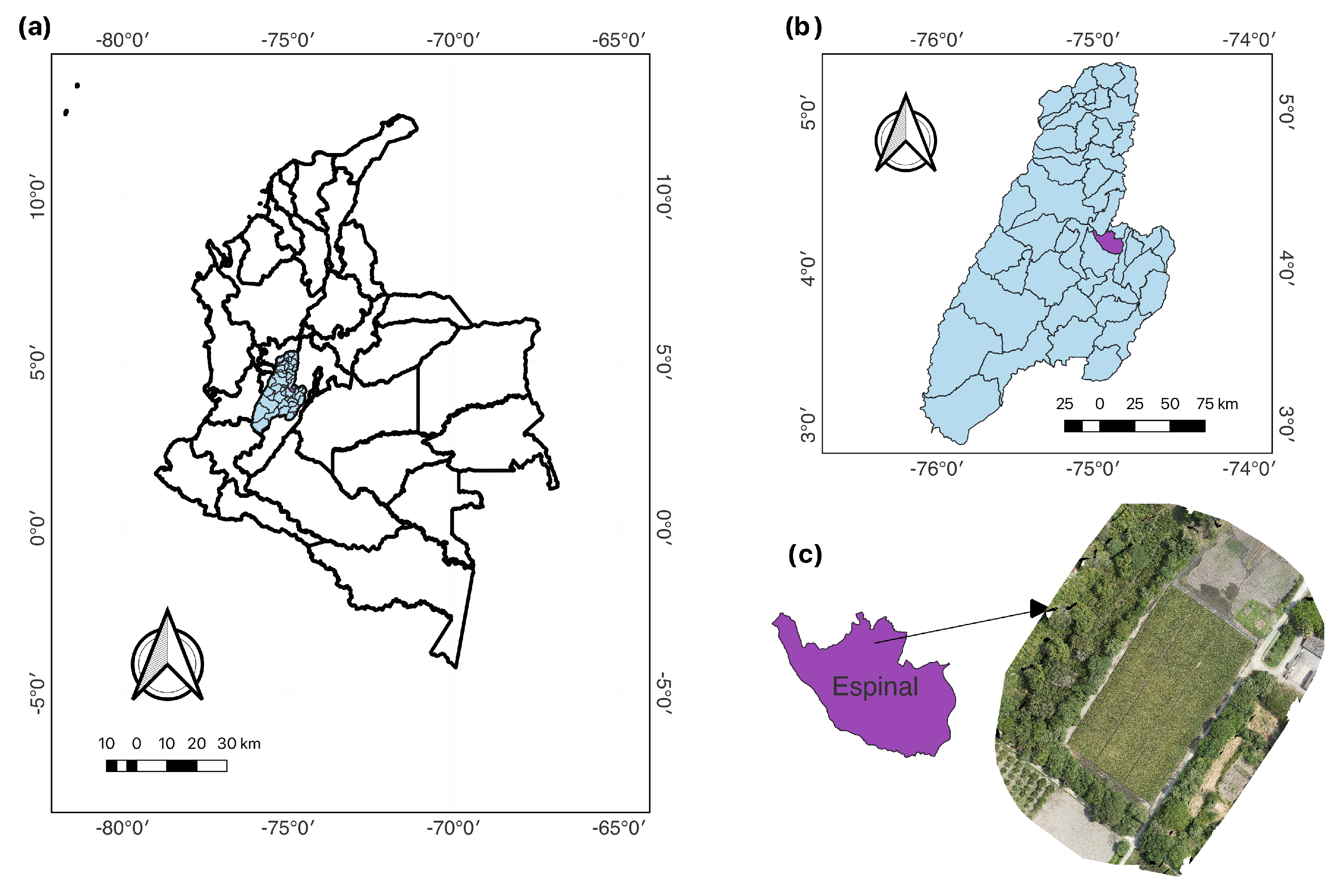
The Tolima region of Colombia hosted the RiceClimaRemote research project. It was a collaboration between ILVO, the Universidad de Ibagué, and Agrosavia. The project focused on developing and implementing irrigation strategies for rice cultivation. Its goal was to identify methods that were best suited to the region’s climate change conditions while still maintaining crop productivity. To achieve this, the project utilized technological tools and data analysis to monitor spatiotemporal variability at the sub-plot level. Field trials were conducted on a one-hectare plot cultivated with the Fedearroz 67 rice variety (Oryza sativa L.) at the Nataima Research Centre of Agrosavia. The research center is in the Espinal municipality of the Tolima region, Colombia (see Figure 2). Trials were conducted in two cycles, during the second semester of 2021 and the first semester of 2022. Three different irrigation techniques were established: multiple inlet rice irrigation (MIRI) [43], alternate wetting and drying (AWD) [44], and conventional flooded irrigation (CONTROL). The experimental area was divided into three strip plots, which enabled the analysis of each treatment.

The multi-temporal image acquisition stage was conducted during sunny and cloudless weather conditions to monitor the crop status. During both the vegetative and reproductive stages, flights were executed biweekly, whereas during the ripening stage, flights took place weekly. RGB images were collected and aligned with multispectral images.

Table 2. RiceClimaRemote VIs. The wavelengths of B, G, R, RE, and NIR are 475, 560, 668, 717, and 842 nm, respectively.

VI	Name	Equation
NDVI	Normalized Difference Vegetation Index [45]	${\displaystyle \frac{NIR-R}{NIR+R}}$
GNDVI	Green Normalized Difference Vegetation Index [46]	${\displaystyle \frac{NIR-G}{NIR+G}}$
NDRE	Normalized Difference Red Edge [47]	${\displaystyle \frac{NIR-RE}{NIR+RE}}$
SAVI	Soil Adjusted Vegetation Index [48]	${\displaystyle \frac{1.5(NIR-R)}{NIR+R+0.5}}$
OSAVI	Optimized Soil Adjusted Vegetation Index [49]	${\displaystyle \frac{1.16(NIR-R)}{NIR+R+0.16}}$
SR	Simple Ratio [50]	${\displaystyle \frac{NIR}{R}}$
GVI	Green Normalized Difference [33]	${\displaystyle \frac{NIR}{G}}$
ExG	Excess Green [32]	$2G-R-B$
GA	Green Area [51]	$60<HUE<180$
GGA	Greener Area [51]	$80<HUE<180$

presents the multispectral and RGB indices obtained. In addition, to monitor the water status of the rice crop, various physiological parameters were measured. Gas exchange, including stomatal conductance (Gs), net photosynthesis rate (Pn), intercellular CO₂ concentration (Ci), and transpiration rate (E), were measured. Additionally, plant samples from a defined area were collected, and the leaf area index was indirectly determined by measuring the fresh and dry weight of a known leaf area. Furthermore, the equivalent water thickness (EWT) was calculated. Canopy water content (CWC) was then calculated using EWT and the leaf area index (LAI). Additionally, the photochemical reflectance index (PRI) was determined using a proximal sensor. In summary, an input feature matrix with $P=22$ features and $N=768$ samples are collected.

3. Experiments and Results

3.1. Training Details, Assessment, and Method Comparison

The baseline SVD-based biplot and our Local Biplot are tested to identify and visualize relevant variables and samples from input features in $\mathbf{X}$. Moreover, we compute the Pearson correlation ${\varrho }_{p{p}^{\prime }}\in [-1,1]$ between features as follows:

$${\varrho }_{p{p}^{\prime }}={\displaystyle \frac{{\langle {\mathit{\xi }}_p-{\overline{\xi }}_p\mathbf{1},{\mathit{\xi }}_{p^{\prime }}-{\overline{\xi }}_{p^{\prime }}\mathbf{1}\rangle }_2}{{\parallel {\mathit{\xi }}_p-{\overline{\xi }}_p\mathbf{1}\parallel }_2{\parallel {\mathit{\xi }}_{p^{\prime }}-{\overline{\xi }}_{p^{\prime }}\mathbf{1}\parallel }_2}},$$

(10)

where ${\mathit{\xi }}_p\in {\mathbb{R}}^N$ holds the p-th column in $\mathbf{X}$, ${\overline{\xi }}_p=\frac{1}{N}{\sum }_{n=1}^N{\xi }_{pn},$ and $p,p^{\prime }\in P.$ A Local Biplot-based feature correlation ${\tilde{\varrho }}_{p{p}^{\prime }}\in [-1,1]$ is computed for a given matched basis matrix by replacing ${\mathit{\xi }}_p$ as the p-th row $\tilde{\mathbf{b}}\in {\mathbb{R}}^2$ of $\tilde{\mathbf{B}}$ in Equation (10). The feature relevance is also computed as in Equation (9). The latter aims to compare the input features linear relationships vs. our Local Biplot-based enhancement to code non-linear dependencies. The number of groups $\tilde{R}$ is fixed as three, four, and five for the Multivariate Guassians, Forage Grasses, and RiceClimaRemote datasets, respectively.

Further, the LR and RF algorithms are used to predict the breeding score (Forage Grasses) and CWC (RiceClimaRemote). The goal is to train two regression models using the complete dataset and our Local Biplot framework to study non-linear and non-stationary behaviors in PA tasks. Next, to quantitatively assess the predictive performance on unseen samples, the coefficient of determination (${\breve{R}}^2$) is reported on the testing set within a five-fold cross-validation scheme. The ${\breve{R}}^2$ is defined as [52]:

$${\breve{R}}^2(\mathbf{y},\widehat{\mathbf{y}})=1-{\displaystyle \frac{\parallel \mathbf{y}-\widehat{\mathbf{y}}{\parallel }_2^2}{\parallel \mathbf{y}-\overline{y}{\mathbf{1}\parallel }_2^2}},$$

(11)

where $\mathbf{y},\widehat{\mathbf{y}}\in {\mathbb{R}}^N$ gather the ground-truth and predicted outputs, respectively, and $\overline{y}=\frac{1}{N}{\sum }_{n=1}^N{y}_n$. A grid-search approach optimizes the hyperparameters of the LR and RF algorithms to sidestep overfitting. For the RF model, we tested different values for the number of trees $\{5,10,50,200\}$ and the maximum number of levels in each decision tree $\{5,10,50,200\}$. In the case of LR, only the intercept parameter was tuned. All experiments were conducted in Python 3.10.12, with the Scikit learn 1.4.2 API, in a Google Colaboratory environment. Our Python codes are publicly available at [53] (accessed on 21 March 2024). Regarding the Forage Grasses database, we use the publicly available data from [30] (accessed on 19 December 2023). The RiceClimaRemote dataset is not available to the public due to privacy considerations.

3.2. Multivariate Gaussians Results

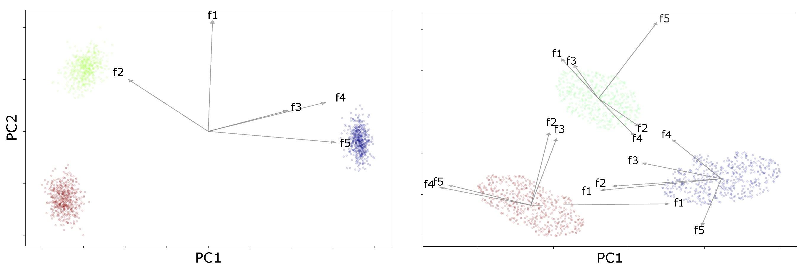
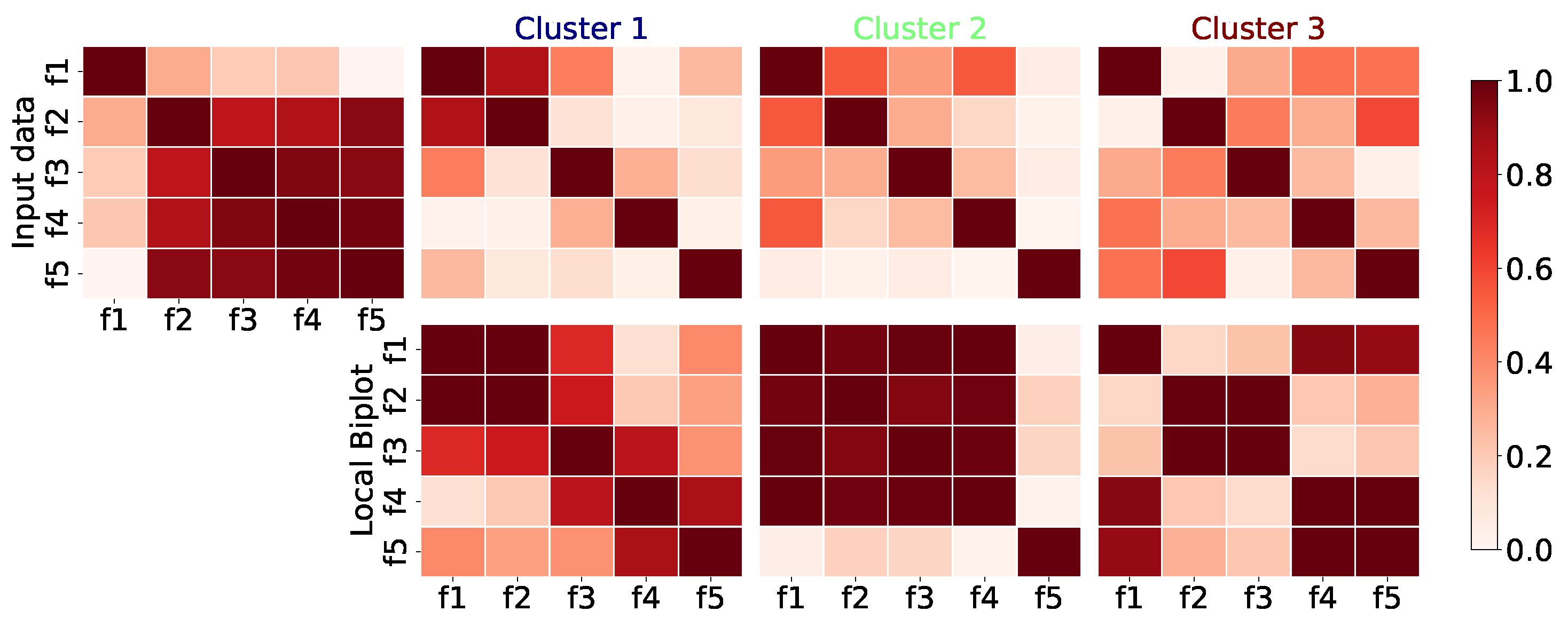
We initially conducted a controlled experiment to evaluate the feasibility of our Local Biplot on synthetic data. Figure 3 displays a traditional SVD-based biplot next to our proposal. We represent features as arrows and depict observations as data points. Both projections are normalized between 0 and 1 for ease of interpretation and visual comparison. Furthermore, in Figure 4 (first row), a panel of input features with absolute Pearson correlation matrices showcases values for both the complete database and each cluster. The second row depicts the same analysis employing Local Biplot.

3.3. Forage Grasses Dataset Results

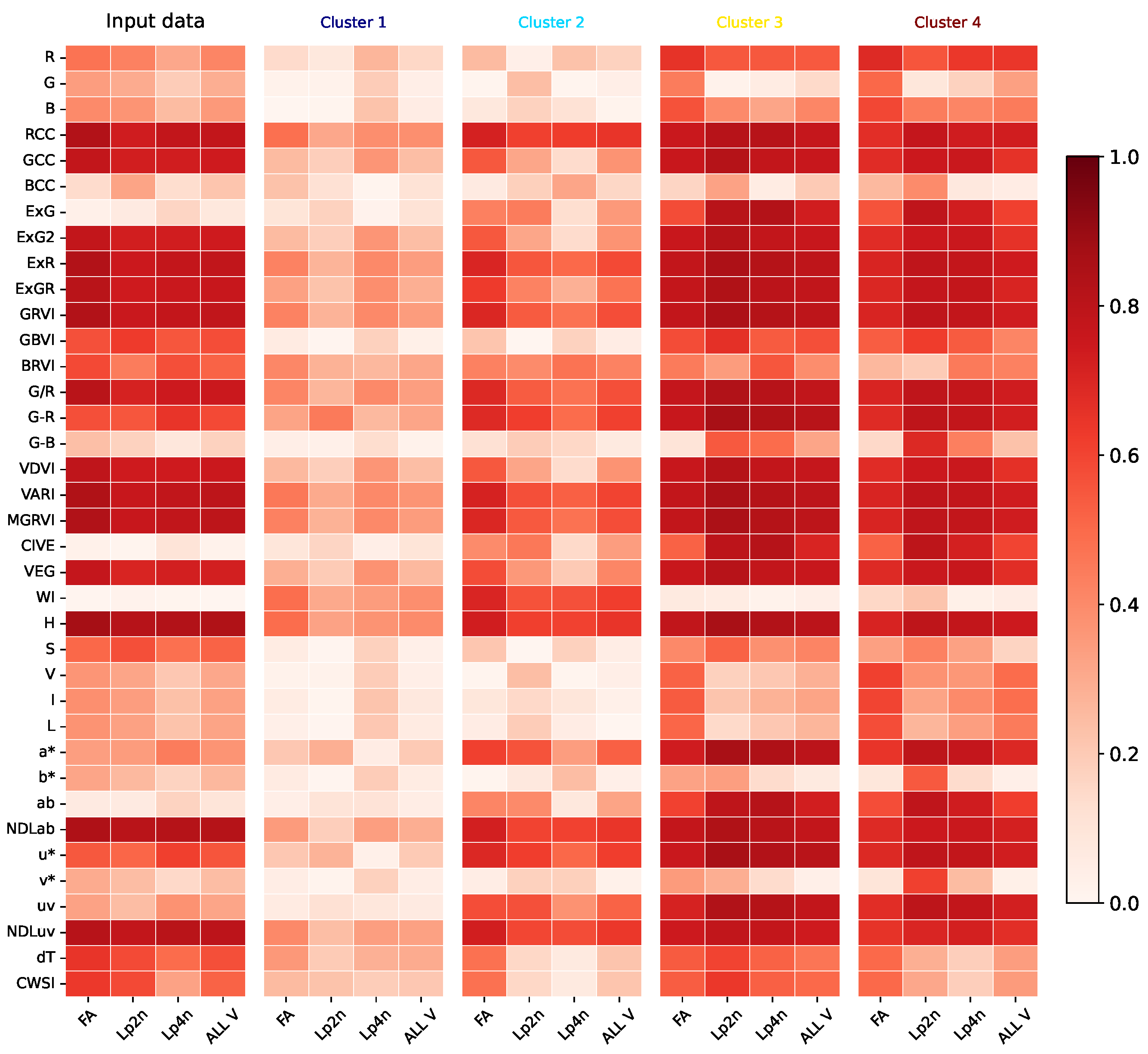
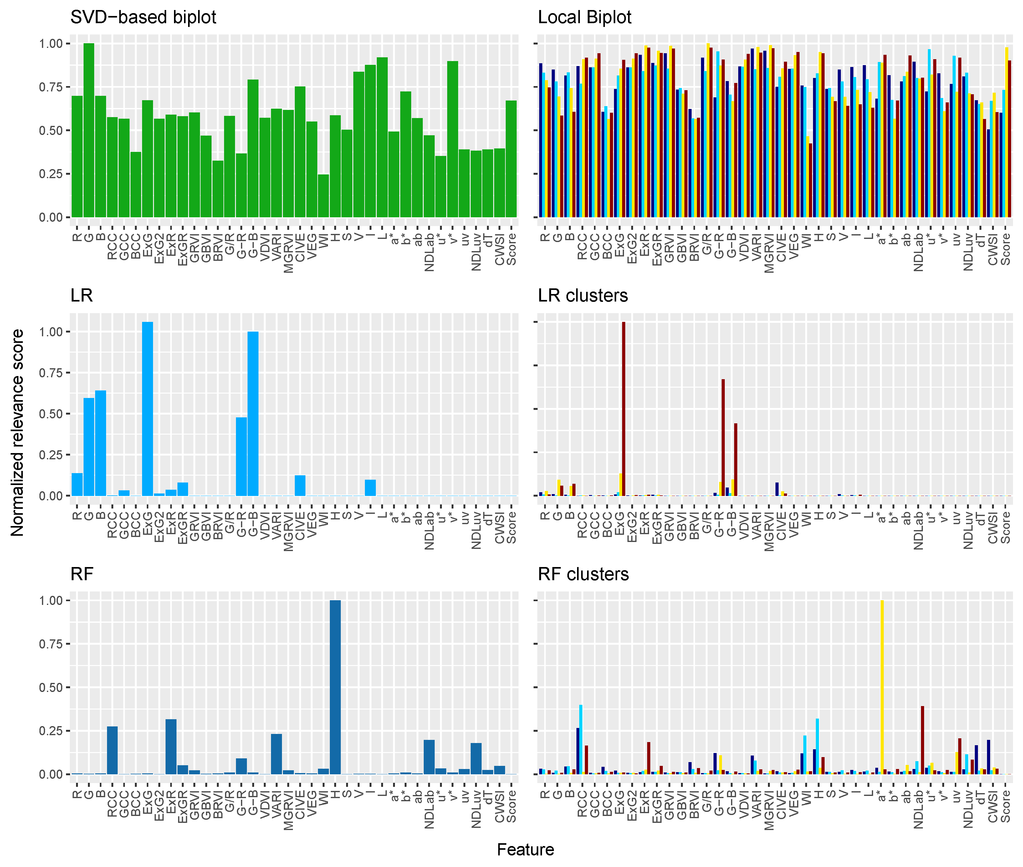
Figure 5 shows the visual inspection results on the Forage Grasses dataset. To illustrate, the basis (depicted as arrows) is presented. The 2D projections using the breeding score as color to provide further insights are also given. The principal components in the projections have been scaled to a range between 0 and 1 for easier interpretation and visual comparison. Then, we found the absolute Pearson correlation between each of the 37 indices and the breeding score. This is shown in Figure 6 and Figure 7 for the SVD-based biplot baseline and our Local Biplot. Each panel displays correlations for individuals, for all species (ALL V), and for the three species (FA, Lp2n, and Lp4n) across all dates, taking into account both the original input features and clustered samples.

Table 3. Forage Grasses breeding score prediction results. Regression performance (average ± standard deviation) regarding the ${\breve{R}}^2$ is computed for all data and for each cluster as provided by our Local Biplot framework (see Figure 5). Cluster size is also depicted. Each cluster header is color-coded and ordered from highest to lowest ${\breve{R}}^2$.

Regressor	All Data	Cluster 1	Cluster 2	Cluster 3	Cluster 4
LR	0.76 ± 0.02	0.65 ± 0.04	0.48 ± 0.06	0.44 ± 0.03	0.21± 0.03
RF	0.75 ± 0.02	0.65 ± 0.07	0.56 ± 0.07	0.42 ± 0.06	0.20 ± 0.06
Sample size	3174	966	461	651	1096

presents the ${\breve{R}}^2$ value for breeding score estimation using RF and LR models. These models were trained using the color space and RGB-based VIs from the grass dataset for all data, as well as for each cluster obtained with our Local Biplot. Figure 8 displays the input feature relevance analysis for the SVD-based biplot, our Local Biplot approach, and the regressor weights (LR and RF). Cluster-based relevance is also provided. For clarity, feature relevance is depicted between 0 and 1 based on a minmaxscaler [52].

3.4. RiceClimaRemote Dataset Results

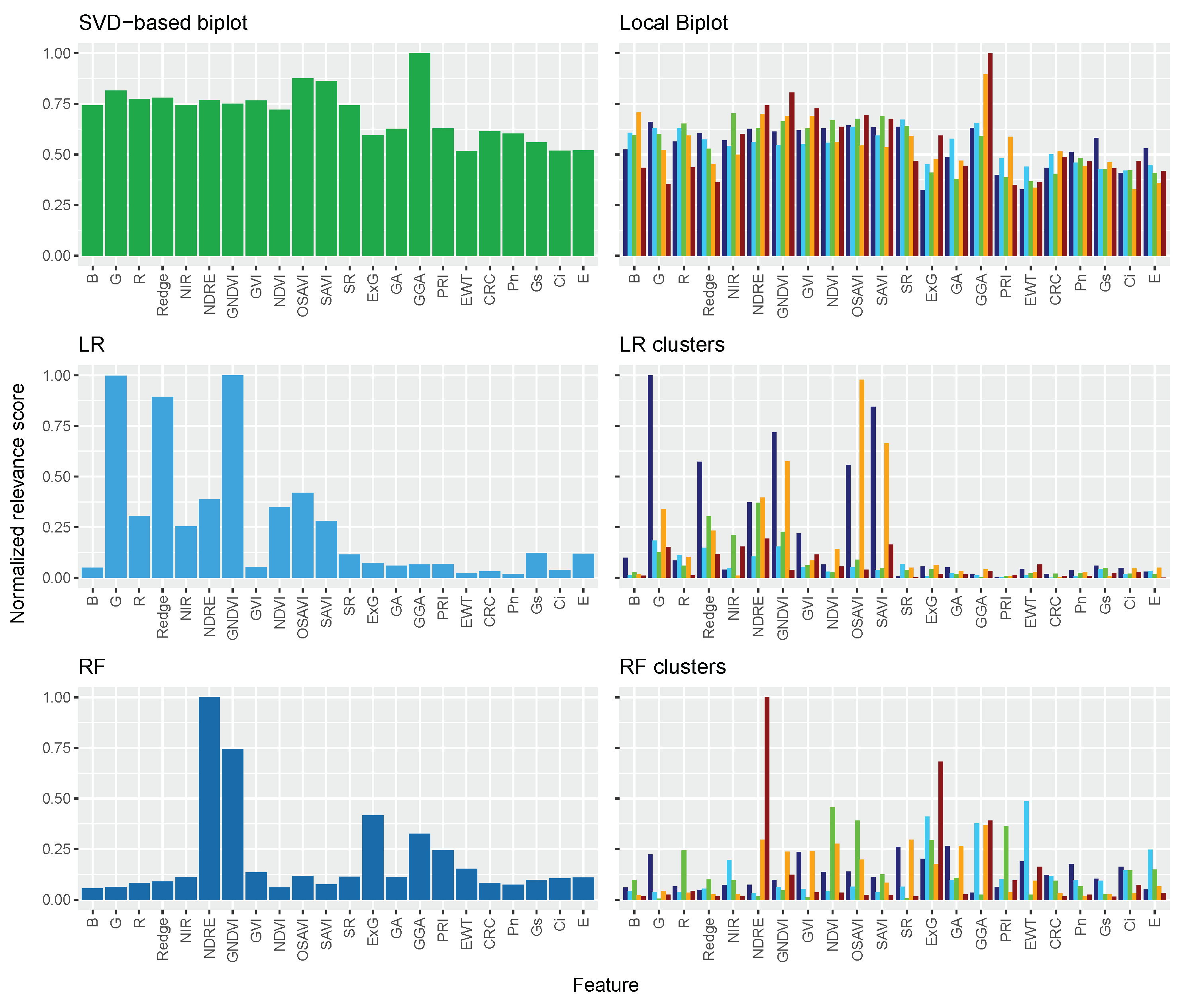
Figure 9 shows the visual inspection results on the RiceClimaRemote dataset. The basis (arrows) are over each projection. Shown also are 2D projections using CWC color. We present the absolute Pearson correlation between each of the 21 variables and the CWC (see Figure 10 and Figure 11). Each panel displays correlations for individuals, for all irrigation treatments (ALL T), and for the three irrigation treatments (MIRI, AWD, CONTROL) across all dates, taking into account both the original input features and clustered samples. Next,

Table 4. RiceClimaRemote CWC prediction results. Regression performance (average ± standard deviation) regarding the ${\breve{R}}^2$ is computed for all data and for each cluster (see Figure 9). Cluster size is also depicted. Each cluster header is color-coded and ordered from highest to lowest ${\breve{R}}^2$.

Regressor	All Data	Cluster 1	Cluster 2	Cluster 3	Cluster 4	Cluster 5
LR	0.55 ± 0.03	0.65 ± 0.16	0.63 ± 0.04	0.45 ± 0.15	0.16 ± 0.18	−1.23 ± 1.14
RF	0.68 ± 0.05	0.67 ± 0.18	0.59 ± 0.06	0.45 ± 0.14	0.28 ± 0.16	−0.97 ± 0.56
Sample size	768	148	195	182	195	48

presents the ${\breve{R}}^2$ values for breeding score estimation. These models were trained using physiological parameters, Multiespectral, and RGB-based VIs for all data and for each cluster. Figure 12 displays the normalized input feature relevance analysis.

4. Discussion

We introduced Local Biplot, a methodological framework designed to visually identify meaningful data patterns within localized contexts over multi-temporal crop data, particularly focusing on water status analysis. Our approach effectively captures data complexity and non-stationarity, enabling the identification and transformation of significant clusters within a common biplot framework for feature-sample contributions.

The results demonstrate that Local Biplot outperforms the traditional SVD-based biplot in identifying and preserving local structures. For instance, in the synthetic dataset, it is clear that the SVD-based embedding depicted in Figure 3 effectively separates the synthetic observations along both principal components. Variables contributing to PC2 have a significant influence on distinguishing the clusters. However, although the classical biplot effectively distinguishes the generated structures, it shows shortcomings in providing explicit insights into the influence of each feature on the respective point clouds. Our local-based biplot method, on the other hand, focuses on capturing local structures and nonlinear relationships in the data. It effectively shows the difference between the structures in the artificially created group samples. The data present a large variation on both axes, and the representation of each variable suggests that the discriminant information may vary between local-based analyses. For instance, while f4 and f5 remain correlated, this correlation breaks in cluster 2. Notably, the classical approach lacks explicit insights into the influence of each feature on the respective point clouds. Pattern variations are evident, as is the correlation change in the Local Biplot embedding. These discrepancies in correlation patterns correspond to different sample subsets produced by multivariate Gaussian distributions. We attribute this success to the combined use of UMAP, clustering, and local SVD decomposition, which preserves both local and global structures, thereby enhancing the ability to capture non-stationary patterns and nonlinearities in the input space. In turn, the Pearson correlation values for the Multivariate Gaussian dataset reveal pattern changes over the entire dataset and within clusters, as shown in Figure 4. The initial clustered data had modest dependencies, but Local Biplot-based correlations enhance them. In cluster 3, the correlation between variables f2 and f4 declined dramatically, while in cluster 1, it increased. Thus, our technique correctly recognized liner and non-linear sample relationships.

For the analysis of the Forage Grasses dataset, Local Biplot’s finer resolution helped a lot in showing how differences between clusters were consistent (see Figure 5). This highlighted the role of visual-based indices in revealing these patterns and suggested potential sources of multicollinearity among indices from various color spaces. For example, the visual-based indices exhibit strong correlation and align with both the left cluster and the score. Thus, the visual appearance seems to play a crucial role in defining and separating the left cluster and the PC2 axis. The PC2 axis, instead, seems to be highly correlated with CIVE, CWSI, dT, a* and G-R. The right cluster displayed higher values on PC1 but exhibited considerable variation across varieties on PC2, suggesting a diverse range of characteristics within this group. Similarly, the left cluster showed variation in PC1. Notably, a relationship exists between both PCs: higher values on PC1 (associated with greener plants) correspond to higher values on PC2 for both clusters.

Further insights were obtained by calculating the absolute Pearson correlation between 37 indices and breeder score (see Figure 6). The high correlation value between the score and the visual-based indices in every cluster emphasizes the RGB color space’s crucial significance in revealing data variability. The consistent patterns of variation depicted by the aligned arrows hint at potential sources of multicollinearity. The lengths of arrows in the biplot analysis indicate that cluster 1 (dark blue) prioritizes variables like VARI, MGRVI, and ExR, while cluster 2 (cyan) focuses on G-R, u*, and uv. Clusters 3 (yellow) and 4 (brown), on the other hand, place higher importance on G/R, GRVI, MGRVI, VARI, and ExR (demonstrating similar values). Furthermore, CWSI holds less significance in cluster 1, and BRVI is less important in cluster 2. Similarly, WI shows lesser significance for clusters 3 and 4.

Additionally, Local Biplot-based correlations in Figure 7 report significant insights into the relationship between VIs, cluster groups, and breeder scores. Each correlation panel, spanning all species (ALL V) and specific species (FA, Lp2n, Lp4n), provided a comprehensive view of feature dependencies considering both the original input data and clustered data. Interestingly, the analysis revealed lower correlations between breeder scores and certain VIs such as R, G, B, RCC, ExR, CIVE, a*, ab, u*, and uv across all clusters compared to the complete dataset. Nonetheless, some visual-based indices like GCC, ExG2, ExGR, GRVI, and G/R showed no clear cluster effect on the linear regressions with breeder scores, resulting in similar correlations across all species except for Lp4n in cluster 2. Moreover, H, NDLAB, and NDLuv exhibited consistent patterns with high correlations in clusters 2, 3, and 4. Notably, Lp2n in cluster 1 and Lp4n in cluster 3 demonstrated greater variation in correlations, mirroring the trends seen across all varieties in cluster 4. These findings are consistent with the relevance bars shown in Figure 8. Furthermore, the reported behaviors highlight the complex interplay between VIs, breeder scores, and genetic or environmental factors, underscoring the importance of detailed and contextual analysis for a comprehensive understanding of drought tolerance in the studied grass species.

Regarding the breeding score prediction, both the LR and RF models generally show similar ${\breve{R}}^2$ values across clusters and the entire dataset (see Table 3). Thus, both models perform comparably in terms of explaining the variability in the target variable based on the input features. Moreover, we observe that high ${\breve{R}}^2$ values are reported for the entire dataset compared to individual clusters. However, cluster 3 has the highest ${\breve{R}}^2$, indicating better predictive performance. Similarly, clusters 2 and 4 exhibit similar predictions, indicating comparable model performance in capturing variability in the target variable within these clusters. In contrast, cluster 1 consistently presents the lowest performance, suggesting potential challenges in model performance. It is worth noting that despite cluster 1 having a larger cluster size, the model struggles with the imbalance in the target values, as seen in Figure 5. It is worth noting that our regression models on all the data outperform the approach presented in ref. [30], where ${\breve{R}}^2$ values were reported between the breeder score and individual VI’s. Figure 8 shows the normalized feature relevance results. As shown, for the complete dataset, the SVD-based biplot provides higher relevance values for all variables than LR and RF relevance values. Note that the RF requires fewer features to achieve similar performance as the LR.

In turn, the examination of the RiceClimaRemote dataset revealed significant complexity and variability (see Figure 9). The SVD-based biplot analysis reveals that although PC1 and PC2 capture much of the data’s variability, the sample points are more dispersed compared to the local-based biplot. GGA, R, B, G, and the highly correlated multispectral indices SR, NDVI, GNDVI, NDRE, and GVI primarily compose PC1. Similarly, PC2 is mainly associated with the NIR band, OSAVI, SAVI, Red Edge, and PRI. This structure suggests a complex data arrangement, with variables exhibiting a significant degree of variability, possibly indicating multiple subgroups or non-stationary patterns within the main group. In contrast, in the local-based biplot, the preservation of local structures leads to the formation of tighter clusters, highlighting subgroups. The resulting 2D non-linear projection (scaled to a range between 0 and 1) captures much of the large-scale global structure. Still, it also preserves the important local structure of the dataset, resulting in five tightly clustered groups. Furthermore, it is notable that multispectral indices such as SR, NDVI, GNDVI, NDRE, and GVI remain highly correlated across all clusters. Additionally, the embedding space underscores the temporal influence on the relationships between features, with distinct contours aligning with different rice growth stages. This temporal dimension is crucial for understanding seasonal variations and other time-dependent factors impacting the rice fields.

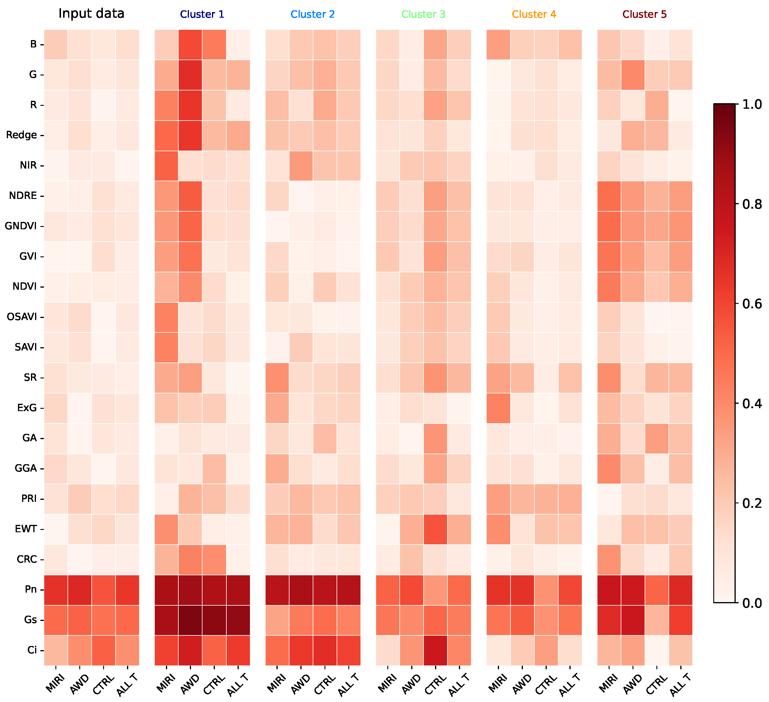
Correlation analyses (Figure 10 and Figure 11) show significant positive correlations between CWC and physiological measurements like Pn and Gs, while Ci’s correlation with CWC varies across clusters. Cluster-specific variations indicate that local data structures significantly influence these relationships, which are not uniformly captured in global analyses. The consistency of correlations among multispectral indices across all clusters suggests robust relationships that persist despite local variations. To understand the interactions among the features within the clusters obtained using our Local Biplot, Figure 11 displays the relationships CWC. This analysis revealed variations in the correlations, with some increasing and others decreasing. In fact, the ${\breve{R}}^2$ measures for CWC estimation presented in Table 4 reveal that cluster 1 (brown) exhibits the highest predictive accuracy for both LR (${\breve{R}}^2=0.65$) and RF (${\breve{R}}^2=0.67$) regressors, emphasizing the importance of local structures in improving model performance. Interestingly, cluster size does not directly correlate with ${\breve{R}}^2$ values, highlighting the complexity of the data and the influence of sample diversity on model performance. For example, cluster 5’s (dark blue) small size hinders the identification of robust data patterns, leading to poor performance and contributing to problems of reproducibility.

Finally, the relevance analysis (Figure 12) indicates that fewer variables are needed for accurate CWC predictions in LR and RF models compared to SVD. The selection of significant spectral bands varies across models, with RF identifying a broader range of important features, contributing to higher prediction accuracy. The variability in feature importance across clusters further demonstrates the heterogeneous nature of the data and the necessity of tailored analysis approaches for different subgroups. These changes can be attributed to the clustering of the UMAP projection within the Local Biplot, which effectively captures the local structure and non-linear relationships. Our framework isolates subsets of points that share similar characteristics.

5. Conclusions

We introduced a methodological framework termed Local Biplot to discern meaningful data patterns within localized contexts, specifically focusing on water status analysis in crops. LocalBiplot captures non-linear and non-stationarity data relationships, allowing us to identify significant clusters for transformation and projection within a shared biplot. We applied a local affine transformation to map the input feature variability-based rankings to the 2D low-dimensional space, providing a complete picture of the local relationships between variables and samples. So, this framework includes the contributions of features and observations within each cluster in the same figure. This makes it easier to understand how data change over time and helps with evaluating variables related to crop water status. We tested our approach using both synthetic and real-world databases, including structured data from grass and rice crops. Our results show that Local Biplot outperforms the traditional SVD-based biplot in finding and preserving local structures. For example, in the synthetic dataset, our method accurately identified the distinct covariance structures of the three artificially generated cloud points. We attribute this success to the combined use of UMAP, clustering, and local SVD decomposition, which preserve both local and global structures, enhancing the ability to capture non-stationary patterns and nonlinearities in the input space. Furthermore, the method’s application to Forage Grasses and RiceClimaRemote datasets has highlighted the utility of visual-based indices and the significant impact of temporal and treatment variations on the data. Our findings emphasize the importance of considering local structures and nonlinear relationships in data-driven precision agriculture.

As future work, extending the LocalBiplot into a deep learning approach is promising research, as demonstrated by the model introduced in ref. [54] to further improve predictive modeling accuracy and robustness. Our next step is to broaden the research to other crops and geographical regions to evaluate the generalizability of the findings [55]. Different crops may exhibit unique data patterns and responses to environmental factors, necessitating tailored approaches for precision agriculture [14]. Additionally, collaborating with agricultural practitioners and stakeholders will help validate the effectiveness of the proposed approaches in other practical settings.

References

1. Arouna, A.; Dzomeku, I.K.; Shaibu, A.G.; Nurudeen, A.R. Water management for sustainable irrigation in rice (Oryza sativa L.) production: A review. Agronomy 2023, 13, 1522. [Google Scholar] [CrossRef]
2. Oumarou Abdoulaye, A.; Lu, H.; Zhu, Y.; Alhaj Hamoud, Y.; Sheteiwy, M. The global trend of the net irrigation water requirement of maize from 1960 to 2050. Climate 2019, 7, 124. [Google Scholar] [CrossRef]
3. Gui, Y.W.; Sheteiwy, M.S.; Zhu, S.G.; Batool, A.; Xiong, Y.C. Differentiate effects of non-hydraulic and hydraulic root signaling on yield and water use efficiency in diploid and tetraploid wheat under drought stress. Environ. Exp. Bot. 2021, 181, 104287. [Google Scholar] [CrossRef]
4. Al Hamedi, F.; Karthishwaran, K.; Alyafei, M.A.M. Hydroponic wheat production using fresh water and treated wastewater under the semi-arid region. Emir. J. Food Agric 2021, 33, 178. [Google Scholar] [CrossRef]
5. Jiang, H.; Hu, H.; Li, B.; Zhang, Z.; Wang, S.; Lin, T. Understanding the non-stationary relationships between corn yields and meteorology via a spatiotemporally varying coefficient model. Agric. For. Meteorol. 2021, 301, 108340. [Google Scholar] [CrossRef]
6. Archana, S.; Kumar, P.S. A Survey on Deep Learning Based Crop Yield Prediction. Nat. Environ. Pollut. Technol. 2023, 22. [Google Scholar] [CrossRef]
7. Crusiol, L.G.T.; Nanni, M.R.; Furlanetto, R.H.; Sibaldelli, R.N.R.; Sun, L.; Gonçalves, S.L.; Foloni, J.S.S.; Mertz-Henning, L.M.; Nepomuceno, A.L.; Neumaier, N.; et al. Assessing the sensitive spectral bands for soybean water status monitoring and soil moisture prediction using leaf-based hyperspectral reflectance. Agric. Water Manag. 2023, 277, 108089. [Google Scholar] [CrossRef]
8. Efthimiou, N. Object-oriented soil erosion modelling: A non-stationary approach towards a realistic calculation of soil loss at parcel level. Catena 2023, 222, 106816. [Google Scholar] [CrossRef]
9. Ndlovu, H.S.; Odindi, J.; Sibanda, M.; Mutanga, O.; Clulow, A.; Chimonyo, V.G.; Mabhaudhi, T. A comparative estimation of maize leaf water content using machine learning techniques and unmanned aerial vehicle (UAV)-based proximal and remotely sensed data. Remote Sens. 2021, 13, 4091. [Google Scholar] [CrossRef]
10. Abdulraheem, M.I.; Zhang, W.; Li, S.; Moshayedi, A.J.; Farooque, A.A.; Hu, J. Advancement of remote sensing for soil measurements and applications: A comprehensive review. Sustainability 2023, 15, 15444. [Google Scholar] [CrossRef]
11. Gu, Z.; Qi, Z.; Burghate, R.; Yuan, S.; Jiao, X.; Xu, J. Irrigation scheduling approaches and applications: A review. J. Irrig. Drain. Eng. 2020, 146, 04020007. [Google Scholar] [CrossRef]
12. Xie, X.; Yang, Y.; Li, W.; Liao, N.; Pan, W.; Su, H. Estimation of Leaf Area Index in a Typical Northern Tropical Secondary Monsoon Rainforest by Different Indirect Methods. Remote Sens. 2023, 15, 1621. [Google Scholar] [CrossRef]
13. Buthelezi, S.; Mutanga, O.; Sibanda, M.; Odindi, J.; Clulow, A.D.; Chimonyo, V.G.; Mabhaudhi, T. Assessing the prospects of remote sensing maize leaf area index using UAV-derived multi-spectral data in smallholder farms across the growing season. Remote Sens. 2023, 15, 1597. [Google Scholar] [CrossRef]
14. Karunathilake, E.; Le, A.T.; Heo, S.; Chung, Y.S.; Mansoor, S. The path to smart farming: Innovations and opportunities in precision agriculture. Agriculture 2023, 13, 1593. [Google Scholar] [CrossRef]
15. Sobjak, R.; De Souza, E.G.; Bazzi, C.L.; Opazo, M.A.U.; Mercante, E.; Aikes Junior, J. Process improvement of selecting the best interpolator and its parameters to create thematic maps. Precis. Agric. 2023, 24, 1461–1496. [Google Scholar] [CrossRef]
16. Dal Prà, A.; Bozzi, R.; Parrini, S.; Immovilli, A.; Davolio, R.; Ruozzi, F.; Fabbri, M.C. Discriminant analysis as a tool to classify farm hay in dairy farms. PLoS ONE 2023, 18, e0294468. [Google Scholar] [CrossRef] [PubMed]
17. Arevalo-Ramirez, T.; Auat Cheein, F. Cluster Analysis for Agriculture. In Encyclopedia of Smart Agriculture Technologies; Zhang, Q., Ed.; Springer International Publishing: Cham, Switzerland, 2022; pp. 1–8. [Google Scholar] [CrossRef]
18. Prakash, S.; Reddy, S.S.; Chaudhary, S.; Vimal, S.; Kumar, A. Multivariate analysis in rice (Oryza sativa L.) germplasms for yield attributing traits. Plant Sci. Today 2024, 11, 64–75. [Google Scholar] [CrossRef]
19. Fu, Z.; Zhang, J.; Jiang, J.; Zhang, Z.; Cao, Q.; Tian, Y.; Zhu, Y.; Cao, W.; Liu, X. Using the time series nitrogen diagnosis curve for precise nitrogen management in wheat and rice. Field Crop. Res. 2024, 307, 109259. [Google Scholar] [CrossRef]
20. Derraz, R.; Muharam, F.M.; Nurulhuda, K.; Jaafar, N.A.; Yap, N.K. Ensemble and single algorithm models to handle multicollinearity of UAV vegetation indices for predicting rice biomass. Comput. Electron. Agric. 2023, 205, 107621. [Google Scholar] [CrossRef]
21. Satpathi, A.; Setiya, P.; Das, B.; Nain, A.S.; Jha, P.K.; Singh, S.; Singh, S. Comparative analysis of statistical and machine learning techniques for rice yield forecasting for Chhattisgarh, India. Sustainability 2023, 15, 2786. [Google Scholar] [CrossRef]
22. Gabriel, K.R. The biplot graphic display of matrices with application to principal component analysis. Biometrika 1971, 58, 453–467. [Google Scholar] [CrossRef]
23. Yan, W.; Tinker, N.A. Biplot analysis of multi-environment trial data: Principles and applications. Can. J. Plant Sci. 2006, 86, 623–645. [Google Scholar] [CrossRef]
24. Mohammadi, R.; Jafarzadeh, J.; Poursiahbidi, M.M.; Hatamzadeh, H.; Amri, A. Genotype-by-environment interaction and stability analysis for grain yield in durum wheat using GGE biplot and genotypic and environmental covariates. Agric. Res. 2023, 12, 364–374. [Google Scholar] [CrossRef]
25. Sharma, V.; Tripathi, A.K.; Mittal, H. Technological revolutions in smart farming: Current trends, challenges & future directions. Comput. Electron. Agric. 2022, 201, 107217. [Google Scholar]
26. Radočaj, D.; Jurišić, M.; Gašparović, M. The role of remote sensing data and methods in a modern approach to fertilization in precision agriculture. Remote Sens. 2022, 14, 778. [Google Scholar] [CrossRef]
27. McInnes, L.; Healy, J.; Melville, J. Umap: Uniform manifold approximation and projection for dimension reduction. arXiv 2018, arXiv:1802.03426. [Google Scholar]
28. Murphy, K.P. Probabilistic Machine Learning: An Introduction; MIT Press: Cambridge, MA, USA, 2022. [Google Scholar]
29. House, D.; Keyser, J.C. Foundations of Physically Based Modeling and Animation; AK Peters/CRC Press: Boca Raton, FL, USA, 2016. [Google Scholar]
30. De Swaef, T.; Maes, W.H.; Aper, J.; Baert, J.; Cougnon, M.; Reheul, D.; Steppe, K.; Roldán-Ruiz, I.; Lootens, P. Applying RGB- and thermal-based vegetation indices from UAVs for high-throughput field phenotyping of drought tolerance in forage grasses. Remote Sens. 2021, 13, 147. [Google Scholar] [CrossRef]
31. Woebbecke, D.M.; Meyer, G.E.; Von Bargen, K.; Mortensen, D.A. Color indices for weed identification under various soil, residue, and lighting conditions. Trans. ASAE 1995, 38, 259–269. [Google Scholar] [CrossRef]
32. Meyer, G.E.; Hindman, T.W.; Laksmi, K. Machine vision detection parameters for plant species identification. In Precision Agriculture and Biological Quality; SPIE: Paris, France, 1999; Volume 3543, pp. 327–335. [Google Scholar]
33. Gitelson, A.A.; Kaufman, Y.J.; Stark, R.; Rundquist, D. Novel algorithms for remote estimation of vegetation fraction. Remote Sens. Environ. 2002, 80, 76–87. [Google Scholar] [CrossRef]
34. Meyer, G.E.; Neto, J.C.; Jones, D.D.; Hindman, T.W. Intensified fuzzy clusters for classifying plant, soil, and residue regions of interest from color images. Comput. Electron. Agric. 2004, 42, 161–180. [Google Scholar] [CrossRef]
35. Genno, H.; Kobayashi, K. Apple growth evaluated automatically with high-definition field monitoring images. Comput. Electron. Agric. 2019, 164, 104895. [Google Scholar] [CrossRef]
36. Jiménez-Muñoz, J.C.; Sobrino, J.A.; Plaza, A.; Guanter, L.; Moreno, J.; Martínez, P. Comparison between fractional vegetation cover retrievals from vegetation indices and spectral mixture analysis: Case study of PROBA/CHRIS data over an agricultural area. Sensors 2009, 9, 768–793. [Google Scholar] [CrossRef] [PubMed]
37. Steele, M.R.; Gitelson, A.A.; Rundquist, D.C.; Merzlyak, M.N. Nondestructive estimation of anthocyanin content in grapevine leaves. Am. J. Enol. Vitic. 2009, 60, 87–92. [Google Scholar] [CrossRef]
38. Xiaoqin, W.; Miaomiao, W.; Shaoqiang, W.; Yundong, W. Extraction of vegetation information from visible unmanned aerial vehicle images. Trans. Chin. Soc. Agric. Eng. 2015, 31. [Google Scholar]
39. Bendig, J.; Yu, K.; Aasen, H.; Bolten, A.; Bennertz, S.; Broscheit, J.; Gnyp, M.L.; Bareth, G. Combining UAV-based plant height from crop surface models, visible, and near infrared vegetation indices for biomass monitoring in barley. Int. J. Appl. Earth Obs. Geoinf. 2015, 39, 79–87. [Google Scholar] [CrossRef]
40. Kataoka, T.; Kaneko, T.; Okamoto, H.; Hata, S. Crop growth estimation system using machine vision. In Proceedings of the 2003 IEEE/ASME International Conference on Advanced Intelligent Mechatronics (AIM 2003), Kobe, Japan, 20–24 July 2003; IEEE: Piscataway, NJ, USA, 2003; Volume 2, pp. b1079–b1083. [Google Scholar]
41. Hague, T.; Tillett, N.; Wheeler, H. Automated crop and weed monitoring in widely spaced cereals. Precis. Agric. 2006, 7, 21–32. [Google Scholar] [CrossRef]
42. Buchaillot, M.L.; Gracia-Romero, A.; Vergara-Diaz, O.; Zaman-Allah, M.A.; Tarekegne, A.; Cairns, J.E.; Prasanna, B.M.; Araus, J.L.; Kefauver, S.C. Evaluating maize genotype performance under low nitrogen conditions using RGB UAV phenotyping techniques. Sensors 2019, 19, 1815. [Google Scholar] [CrossRef] [PubMed]
43. Vories, E.; Tacker, P.; Hogan, R. Multiple inlet approach to reduce water requirements for rice production. Appl. Eng. Agric. 2005, 21, 611–616. [Google Scholar] [CrossRef]
44. Rejesus, R.M.; Palis, F.G.; Rodriguez, D.G.P.; Lampayan, R.M.; Bouman, B.A. Impact of the alternate wetting and drying (AWD) water-saving irrigation technique: Evidence from rice producers in the Philippines. Food Policy 2011, 36, 280–288. [Google Scholar] [CrossRef]
45. Kriegler, F.J. Preprocessing transformations and their effects on multspectral recognition. In Proceedings of the Sixth International Symposium on Remote Sesning of Environment, Ann Arbor, MI, USA, 13–16 October 1969; pp. 97–131. [Google Scholar]
46. Shaver, T.; Khosla, R.; Westfall, D. Utilizing green normalized difference vegetation indices (GNDVI) for production level management zone delineation in irrigated corn. In Proceedings of the 18th World Congress of Soil Science, Philadelphia, PA, USA, 9–15 July 2006. [Google Scholar]
47. Sharifi, A.; Felegari, S. Remotely sensed normalized difference red-edge index for rangeland biomass estimation. Aircr. Eng. Aerosp. Technol. 2023, 95, 1128–1136. [Google Scholar] [CrossRef]
48. Huete, A.R. A soil-adjusted vegetation index (SAVI). Remote Sens. Environ. 1988, 25, 295–309. [Google Scholar] [CrossRef]
49. Steven, M.D. The sensitivity of the OSAVI vegetation index to observational parameters. Remote Sens. Environ. 1998, 63, 49–60. [Google Scholar] [CrossRef]
50. Aparicio, N.; Villegas, D.; Casadesus, J.; Araus, J.L.; Royo, C. Spectral vegetation indices as nondestructive tools for determining durum wheat yield. Agron. J. 2000, 92, 83–91. [Google Scholar] [CrossRef]
51. Casadesús, J.; Kaya, Y.; Bort, J.; Nachit, M.; Araus, J.; Amor, S.; Ferrazzano, G.; Maalouf, F.; Maccaferri, M.; Martos, V.; et al. Using vegetation indices derived from conventional digital cameras as selection criteria for wheat breeding in water-limited environments. Ann. Appl. Biol. 2007, 150, 227–236. [Google Scholar] [CrossRef]
52. Géron, A. Hands-on Machine Learning with Scikit-Learn, Keras, and TensorFlow; O’Reilly Media, Inc.: Sebastopol, CA, USA, 2022. [Google Scholar]
53. Triana-Martinez, J.C. Python-gcpds.localbiplot. 2024. Available online: https://github.com/UN-GCPDS/python-gcpds.localbiplot (accessed on 21 March 2024).
54. Wu, L.; Yuan, L.; Zhao, G.; Lin, H.; Li, S.Z. Deep clustering and visualization for end-to-end high-dimensional data analysis. IEEE Trans. Neural Netw. Learn. Syst. 2022, 34, 8543–8554. [Google Scholar] [CrossRef] [PubMed]
55. Wang, H.; Chang, W.; Yao, Y.; Yao, Z.; Zhao, Y.; Li, S.; Liu, Z.; Zhang, X. Cropformer: A new generalized deep learning classification approach for multi-scenario crop classification. Front. Plant Sci. 2023, 14, 1130659. [Google Scholar] [CrossRef]
Figure 1. Local Biplot sketch. Dotted line: cluster-based operation.
Remotesensing 16 02854 g001
Figure 2. RiceClimaRemote dataset site’s location. (a) Colombia; (b) Tolima department; (c) Espinal and experimental field with RGB raster.
Remotesensing 16 02854 g002
Figure 3. Multivariate Gaussians dataset visual inspection results. (Left): SVD-based biplot. (Right): Local Biplot (ours). Gray arrows depict each feature in the dataset (f1–f5), which shed light on their correlations. Examining the scatter points and their colors allows us to visually understand sample distributions. PC stands for principal component (basis).
Remotesensing 16 02854 g003
Figure 4. Multivariate Gaussians: Pearson correlation results. First row: a panel of absolute feature correlation matrices showcases values for both the complete database and each cluster using the SVD-based biplot. The second row displays cluster-specific absolute correlations from our Local Biplot.
Remotesensing 16 02854 g004
Figure 5. Forage Grasses biplots. Left: SVD-based biplot. Middle: Local Biplot. Right: Local Biplot and cluster-based probability boundaries. The colors in the left and middle plots represent the clustering label. The right plot’s color emphasizes the target variable (breeding score), while the flight dates (TF1, TF2, and TF3) determine the color of the curves. PC: principal component (basis).
Remotesensing 16 02854 g005
Figure 6. Forage Grasses Pearson correlation results: SVD-based biplot. We show the absolute correlation between the VIs and the breeding score (target) for each species individually and collectively. We also establish correlations for each cluster separately and throughout the dataset.
Remotesensing 16 02854 g006
Figure 7. Forage Grasses Pearson correlation results: Local Biplot (ours). We show the absolute correlation between the VIs and the breeding score (target) for each species individually and collectively. We also establish correlations for each cluster separately and throughout the dataset.
Remotesensing 16 02854 g007
Figure 8. Forage Grasses feature relevance analysis. SVD-based biplot and Local Biplot (ours) normalized feature relevance are presented. We also show the LR and RF regressor weights. The bar color in the second column stands for the Local Biplot clusters labels (see Figure 5).
Remotesensing 16 02854 g008
Figure 9. RiceClimaRemote biplot results. Left: SVD-based biplot. Middle: Local Biplot. Right: Local Biplot and cluster-based probability boundaries. The colors in the left and middle plots represent the clustering label. The right plot’s color emphasizes the target variable (CWC), while the growth stages of rice (vegetative, reproductive, and ripening) determine the color of the curves. PC: principal component (basis).
Remotesensing 16 02854 g009
Figure 10. RiceClimaRemote Pearson correlation results: SVD-based biplot. For each irrigation treatment, we show the absolute correlation (cluster- and entire-data-based) between the selected feature and the CWC (target), both individually and collectively.
Remotesensing 16 02854 g010
Figure 11. RiceClimaRemote Pearson correlation results: Local Biplot (ours). For each irrigation treatment, we show the absolute correlation (cluster- and entire-data-based) between the selected feature and the CWC (target), both individually and collectively.
Remotesensing 16 02854 g011
Figure 12. RiceClimaRemote feature relevance analysis. SVD-based biplot and Local Biplot (ours) normalized feature relevance are presented. We also present the LR and RF regressor weights. The bar color in the second column stands for the Local Biplot clusters labels (see Figure 9).
Remotesensing 16 02854 g012