SAR Temporal Shifting: A New Approach for Optical-to-SAR Translation with Consistent Viewing Geometry

Abstract

In contrast to the well-investigated field of Synthetic Aperture Radar (SAR)-to-Optical translation, this study explores the lesser-investigated domain of Optical-to-SAR translation, which is a challenging field due to the ill-posed nature of this translation. The complexity arises as single optical data can have multiple SAR representations based on the SAR viewing geometry. To generate an SAR image with a specific viewing geometry, we propose a novel approach, which is termed SAR Temporal Shifting. Our model takes an optical image from the target timestamp and an SAR image from a different temporal point but with a consistent viewing geometry as the expected SAR image. Both of these inputs are complemented with a change map derived from optical images during the intervening period. This model then modifies the SAR data based on the changes observed in the optical data to generate the SAR data for the desired timestamp. Although similar strategies have been explored in the opposite SAR-to-Optical translation, our approach innovates by introducing new spatial evaluation metrics and cost functions. These metrics reveal that simply adding same-domain data as model input, without accounting for the distribution changes in the dataset, can result in model overfitting—even if traditional metrics suggest positive outcomes. To address this issue, we have introduced a change-weighted loss function that discourages the model from merely replicating input data by assigning greater cost to changes in the areas of interest. Our approach surpasses traditional translation methods by eliminating the Generative Adversarial Network’s (GAN’s) fiction phenomenon by learning to change the SAR data based on the optical data instead of solely relying on translation. Furthering the field, we have introduced a novel automated framework to build a despeckled multitemporal SAR–Optical dataset with consistent viewing geometry. We provide the code and the dataset used in our study.

1. Introduction

Generative Adversarial Networks (GANs) have played an increasingly significant role in the field of remote sensing. Among their diverse applications, i.e., semantic segmentation [1], super-resolution [2], and text-to-image generation [3], there has been a notable emphasis on data translation, particularly in the context of image-to-image translation [4]. This technique involves creating mapping functions that connect input and output data [5]. This method finds versatile applications, encompassing Domain Adaptation (DA) and the conversion of diverse remote sensing data sources. Its goal is to enhance model performance in downstream tasks and/or improve the interpretability of data [4].

Translation between Synthetic Aperture Radar (SAR) and Optical data is a significant domain, where image-to-image translation is increasingly applied in remote sensing [4]. The SAR-to-Optical (SAR2Opt) translation serves two primary objectives: first, it aims to enhance the interpretability of SAR data; second, it leverages the all-weather, night–day capabilities of SAR instruments, rendering them invaluable sources for cloud removal tasks [6,7,8] or as an alternative to optical data when they are unavailable due to thick smoke and aerosol layers in the atmosphere [9].

Despite significant advancements in SAR2Opt translation, driven by the advent of GANs, there remains a notable gap in the literature when it comes to a comprehensive analysis of the reverse challenge: the Optical-to-SAR translation (Opt2SAR). This gap is attributed to the inherently challenging nature of the problem, particularly in dealing with the dissimilarity between two SAR images within a single Region of Interest (ROI) when the viewing geometries differ [10]. Nonetheless, achieving a robust model on this side of translation can pave the way for translating legacy optical datasets that have been made prior to an SAR mission. This advancement can also improve downstream tasks, such as the process of detecting changes between heterogeneous SAR images and optical images [9], and contribute to the development of super-resolution spatial/temporal models for SAR images [4]. This is achievable by supplementing low spatial/temporal resolution SAR data with high spatial/temporal resolution optical data, i.e., using optical time series to fill in the gaps in the SAR time series or leveraging it to increase the SAR’s spatial resolution.

A recurring challenge in both SAR2Opt and Opt2SAR translation literature is the “Fiction” phenomenon, which occurs when the reference data lack sufficient information. This deficiency leads the model to supplement their own data, often deviating from the actual ground truth to generate the translated data. The Fiction issue is particularly evident in two areas of an SAR2Opt task. Firstly, the GAN model struggles to restore the actual spectral diversity of the ground truth data, leading to low fidelity in the spectra in the translated optical data [11]. Secondly, the model often fails to retain texture and fine-grained borders in the translated data, as SAR and optical data have fundamentally different structures, resulting in an inaccuracy result with respect to detail [12,13].

Regardless of whether it is an SAR2Opt or an Opt2SAR task, most existing research in this domain has relied on monotemporal SAR–Optical datasets. This means that the algorithms are set to learn the relationship between the SAR and optical domains without additional information. This would require that the SAR and optical data provide similar discrimination of surface targets. However, this is not the case, as surfaces with the same spectral composition can have different backscattering properties and vice versa. To counter this problem, Xiong et al. [8] and He et al. [14], in their SAR2Opt task, concatenated the SAR and optical data of a previous timestamp in order to keep the surface details and to save textural and spectral details in the generated optical data. This is close to the approach taken by He et al. [15], where in their super-resolution task, they incorporated high-resolution data with different timestamps alongside the low-resolution data of the desired timestamp to generate high-resolution data.

Despite the advancements, utilizing data from the same domain as the desired output inherently introduces biases. Regions that are predominantly unchanged compared to those that have been altered can skew the dataset, leading to overfitting where the model tends to replicate the input data instead of learning the underlying transformations. This issue often goes undetected, as conventional metrics may still reflect favorable outcomes due to their averaging effects [16].

This research first introduces new evaluation metrics capable of discerning the aforementioned bias by separately evaluating changed and unchanged regions. Then, we introduce a novel Siamese encoder GAN with attention mechanisms to fuse the optical and SAR branches. Finally, we take an algorithm-level approach to resolve the same-domain input overfitting problem by forcing the model to learn from the optical input image.

To test our model, cost function, and evaluation metrics, as well as to confine the outcomes of this one-to-many translation problem, we created an automated framework to create a cloud–snow-free despeckled bitemporal dataset with consistent SAR incident angles and to generate realistic SAR images with the desired viewing geometry.

We term our methodology as “SAR Temporal Shifting”, which redefines the Opt2SAR translation problem. This approach involves modifying an input SAR image based on temporal changes in optical data to align with a new SAR image from a desired timestamp. Our key contributions are as follows:

• Introduction of viewing-geometry-consistent temporal context in Opt2SAR translation: By integrating SAR and optical data from different timestamps, our approach, termed “SAR Temporal Shifting”, overcomes the limitations of monotemporal datasets by using the SAR input to establish a viewing geometry of the output data and adapting the SAR data in response to observed changes in the optical images.
• Development of novel evaluation metrics: In the evaluation phase, we introduce metrics specifically designed to differentiate between the model’s performance in areas that have undergone changes and those that remain static. This enhancement not only highlights a common flaw in the bitemporal translation approach but also demonstrates how our approach effectively addresses this issue.
• An algorithm-level approach to prevent same-domain overfitting: To account for the inherent imbalance between the altered and intact areas over a short time span, we propose a specialized loss function. This loss function, by assigning different costs to the changed areas, prevents the model from overfitting the input SAR data and merely replicating them as the output.
• Design of an automatic, multitemporal, paired SAR–Optical dataset downloader framework: This workflow automatically selects the optimal Sentinel-1 orbit based on specified criteria and retrieves cloud-free Sentinel-2 optical data. It pairs the optical data with despeckled SAR data, maintaining consistent viewing geometry across all timestamps, to create a well-matched dataset. The framework is easily customizable for different regions, enhancing its utility and integration in future research projects.

2. Related Work

2.1. Generative Adversarial Networks

Generative Adversarial Networks operate on the concept of a min-max game, where both the generator and the discriminator are iteratively refined to reach a Nash equilibrium. The goal is to make the distribution of the generated data closely resemble that of the real data. In this process, the generator produces synthetic data from noise, typically drawn from a uniform or Gaussian distribution. Meanwhile, the discriminator’s role is to discern between outputs from the generator and actual data. The aim of the generator is to better mimic real data, and for the discriminator, it is to enhance its ability to distinguish real data from synthetic data. While GANs are generally effective, they are unsupervised networks, which can sometimes limit the scope and control of the generated outputs [12]. To address this limitation, conditional GANs (CGANs) have been introduced [17]. CGANs incorporate additional conditions, such as labels, data, or text, to constrain the types of generated data. The loss function for a CGAN is defined as follows:

$$\begin{array}{cc}\hfill \underset{G}{min}\underset{D}{max}{\mathcal{L}}_{cGANs}(G,D)=& E[log(D(y,x)\left)\right]+E[log(1-D(y,G(x\left)\right)\left)\right]\hfill \end{array}$$

(1)

In this expression, ${\mathcal{L}}_{cGANs}(G,D)$ is the conditional GAN loss, E represents the expected value, x represents actual data, y indicates the conditional parameters, and $G\left(x\right)$ is the output from the generator. The term $D(y,x)$ is the discriminator’s output when given real data, while $D(y,G(x\left)\right)$ is how the discriminator responds to the generator’s synthetic data.

Image-to-image translation GANs are CGANs in which the imposed condition is the input image. Based on the optimization method and the arrangement of source–target datasets, current GAN-based methods for image-to-image translation can be categorized into two main groups: paired and unpaired methods [9].

The paired methods need a dataset with matching source and target data, i.e., for all source data, there must be target data. A landmark for paired methods is the Pix2Pix [18] architecture. Its generator follows a U-net [19] architecture, while the discriminator employs a patchGAN architecture to model the image as a Markov random field [20].

In contrast to the paired translation, unpaired methods use two unpaired datasets from both domains. A standard method for unpaired methods is the CycleGAN [5], which incorporates a combination of cycle consistency loss and identity loss in the GAN loss function.

2.2. Optical–SAR Translation

The literature on Optical-to-SAR translation can be categorized into two sections: the body of research that focuses on the translation aspect of the problem and the research that aims to harness this method for practical applications. The following subsection contains a review of these categories.

2.2.1. Translation Methods

The comparative evaluation by Zhao et al. in 2022 [9] was performed on various data-to-data translation methods for SAR2Opt translation methods, including the BicycleGAN [21], CycleGAN [5], CUT [22], MUNIT [23], NICE-GAN [24], and Attn-CycleGAN [25]. The evaluation was conducted on the SEN1-2 dataset [26], which is a paired dataset of Sentinel-1 and Sentinel-2 data captured in 2016 and 2017. The dataset was divided into four categories based on seasons, i.e., Winter, Fall, Summer, and Spring. It covers a vast geographical area, whereas the sample points are biased towards urban areas. Furthermore, in their study, Zhao et al. [9] also introduced a novel dataset called SAR2Opt, which consists of paired data from TerraSAR-X and Google Earth. The evaluation results indicate that Pix2Pix and CycleGAN outperformed other models in terms of the peak signal-to-noise ratio (PSNR) and structural similarity index (SSIM). Pix2Pix exhibited the highest PSNR scores across all datasets and the best SSIM in the Winter, Fall, and SAR2Opt datasets. On the other hand, the CycleGAN achieved superior SSIM scores in the Spring and Summer datasets. The authors attributed this distinction to the complexity of the land surface characteristics, for which the CycleGAN’s unpaired approach was better suited. This compelling performance of Pix2Pix has led us to select it as the base model for our study, as discussed in the methodology section of this paper.

Reyes et al. [13] selected the CycleGAN as their base model for SAR2Opt translation, with a primary focus on result interpretability. The authors acknowledged the fundamental limits of SAR2Opt translation that cannot be compensated for, suggesting that learning the transition from single-channel SAR data to multichannel optical data is an inherently challenging, making it an ill-posed problem similar to colorizing grayscale data in classical computer vision. They emphasized that the diversity of surface parameters, such as variability and correlation length, relative permittivity, or geometry—which contribute to unique wavelength- and temperature-dependent signal responses—made the work more challenging. Reyes et al. also identified issues related to the Fiction phenomenon in the translation process. They demonstrated that, in urban areas, while models could be successful in transforming regions with corner reflection into blocks of buildings, the shape and number of buildings in the resulting optical data were different from those in the original data. Another challenge was the separation of agricultural fields, which is immediately discernible in optical data but fades in SAR data and thus their optical translation.

Guo et al. [27] introduced Edge-Preserving Convolutional Generative Adversarial Networks (EPCGANs), enhancing the CycleGAN architecture for SAR-to-Optical image translation. By incorporating edge information and content-adaptive convolutions, EPCGANs improve the structural integrity of the output images while suppressing speckles noise. Tested on the SEN1-2 dataset, their model achieved state-of-the-art (SOTA) results, surpassing previous methods. Notably, their research is among the few that have utilized perceptual loss [28] to enhance SAR-to-Optical image translation.

Zhang et al. [29] introduced a model based on Neural Partial Differential Equations called S2O-NPDE to mitigate geometric distortions in generated optical images and provide an explainable design. They used a module based on the Taylor Central Difference (TCD) in a residual manner as the backbone of their generator, along with a parallel Perona–Malik Diffusion (PMD) module for feature diffusion through layers aimed at removing noise and preserving geometric structures, achieving SOTA results.

A reciprocal Optical–SAR translation study was done by Fu et al. [10], where they introduced a modified Pix2Pix GAN architecture that uses multiscale cascaded residual connections, i.e., the CRAN. They tested their model on both satellite and aerial datasets. They concluded that when using full PolSAR data as input, the results were more favorable compared to using single polarization data. They attributed the discrepancy to the fact that some objects are not visible in single-pol SAR data. Similar to Reyes et al., they found that while land covers like waters and vegetation areas were easily reconstructed, the model struggled to reconstruct built-up areas, resulting in building cubes with edges that were not well-aligned. Furthermore, for tall buildings, the structures were smeared, which they attributed to model confusion due to variable viewing angles.

Intertwined with the discourse presented by Reyes et al., we recognize that the task of translating optical data into SAR data is not a straightforward one-to-one problem due to artifacts introduced by surface topography and the varying viewing geometry of the SAR instrument. Our study provides a comprehensive discussion of the challenges, as well as our approach to overcoming these challenges.

2.2.2. Applications of Optical–SAR Translation

Li et al. presented the Deep Translation network for Change Detection (DTCDN). This network leverages the innovative Nice-GAN architecture as the translation model and incorporates a customized U-Net++ [30] architecture with a multiscale loss function for change detection. In essence, their approach involves the transformation of one type of data, either SAR or optical, to the domain of the other type of data. Subsequently, both translated and original data of another time are fed into the U-Net++ network, which is then trained in a supervised manner to detect changes. In a thorough evaluation of four different datasets, they found that the effectiveness of translation varied: in some cases, translating optical to SAR was more successful, while in others, SAR to optical yielded better results for detecting the change [31].

In a recent study by Hu et al., a comprehensive dataset comprising Sentinel-1 and Sentinel-2 data was employed to successfully showcase the potential of GANs for SAR2Opt translation in the context of over 304 wildfire events. The researchers capitalized on the unique capability of SAR data to capture surface details even in the presence of dense smoke, which tends to obscure optical wavelengths and renders optical data ineffective. To achieve this, the authors employed a ResNet-based Pix2Pix architecture to translate SAR data from both before and after wildfire events. This translation was used to generate burnt severity classification maps and optical burnt indices incorporating all possible combinations of real and synthetic optical data from the two timestamps. Notably, the study found that the generated indices had a stronger correlation with the real optical indices compared to the original SAR-based indices. Furthermore, this approach outperformed SAR-based indices in accurately mapping the extent of burnt areas [32].

3. Bitemporal Dataset

In our study, we recognized the importance of having a consistent multitemporal dataset that could be used to effectively test and refine our methodology. To address this need, we developed two paired datasets consisting of Sentinel-1 Ground Range Detected (GRD) and Sentinel-2 data from the years 2019 and 2021. The Sentinel-1 data exclusively feature the VV polarization, while the Sentinel-2 data comprise RGB and NIR bands at a spatial resolution of 10 m, along with the SWIR-1 and SWIR-2 bands at 20 m. The Sentinel-2 data were obtained from the Level-2A Collection, which includes atmospherically corrected surface reflectance (SR) data derived from the associated Level-1C products.

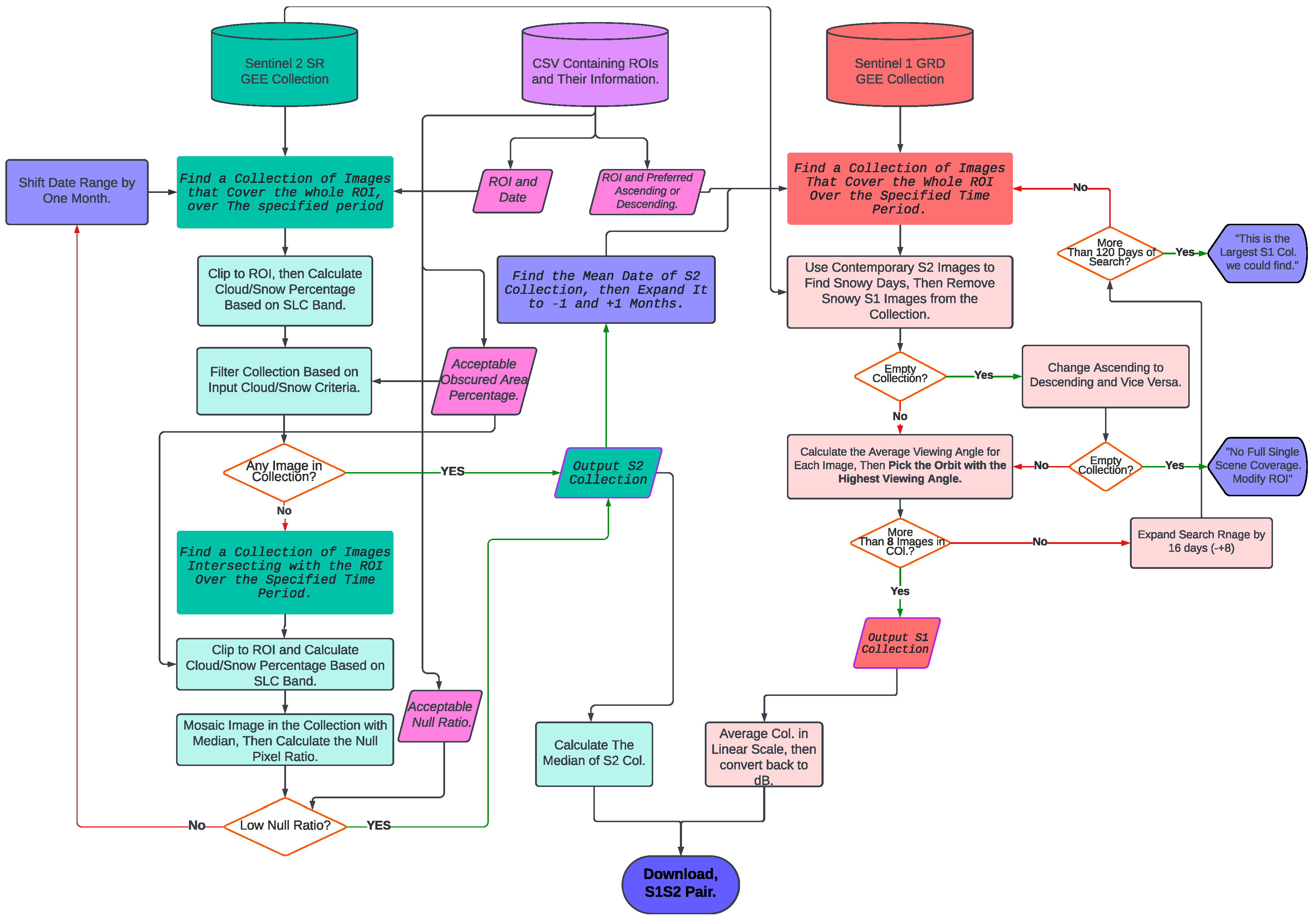
To ensure reproducibility, we developed a semiautomated workflow using the Google Earth Engine [33] Python API and the GeeMap [34] Library. Our workflow, available on GitHub, allows the user to create a paired Sentinel-1 and Sentinel-2 dataset by downloading and patching data for a given set of ROIs and dates. The process requires only a few parameters to be tuned. We will delve into the specific details of this workflow and the resulting dataset in subsequent sections. Figure 1 provides a high-level overview of the workflow.

3.1. Sentinel-2 Data

The process of acquiring Sentinel-2 data through our workflow is relatively straightforward. Given the geographical location and corresponding date of the ROI, the process locates a GEE data collection of that area. The cloud cover of the ROI is calculated using the Scene Classification (SLC) band in the Level-2A Collection [35]. If a scene or data collection is not found with an acceptable level of cloud cover, the process recursively shifts the date by one month until a suitable collection is located.

Once a collection is found, we select either the data with the lowest cloud cover or the median of the data collection, which depends on the amount of data in the collection. This approach ensures that we acquire the most suitable Sentinel-2 data available for each ROI and date.

3.2. Sentinel-1 Data

As previously stated in the introduction, the Opt2SAR translation presents an ill-posed problem where, based on the SAR instrument’s viewing geometry, there are multiple solutions for this translation.

Figure 2 provides a visual representation of this phenomenon depicting two images of ascending data captured over Paris, with different incident angles (The incident angle is the angle between the incoming radar beam and a vector perpendicular to the target [36]). It can be observed that the backscatter values, the shape of the building blocks, and SAR artifacts are different in these two samples of data. In order to address the issue of indeterminate solutions, a set of rules on the selection of the Region of Interest, orbit number, and despeckling was established to constrain the possible outcomes, aiding the GAN model in generating a unified answer for the translation. The following sections will provide a more detailed explanation of how each of these rules has been implemented.

3.2.1. Regions of Interest

SAR data are subject to significant influences from the Earth’s relief [37]. In regions where the relief exhibits high variance, such as hills and valleys, SAR data can be affected by foreshortening, layover, and occlusion. To avoid these issues, we chose to limit the Regions of Interest (ROIs) to urban areas, which are generally flat and exhibit low relief variance. The ROIs were selected using the Onera Satellite Change Detection (OSCD) dataset [38], which includes 24 urban areas from around the world. Of these, 14 were designated for training, and the remaining 10 were reserved for testing. The OSCD dataset was originally developed for change detection analysis of Sentinel-2 data.

To increase the size of the OSCD dataset for training the Generative Adversarial Network, we employed two approaches. Firstly, we expanded the regions to encompass entire urban areas, since some of the original OSCD ROIs represented only a small portion of a city. We carefully selected new ROIs that did not contain hills or valleys in order to avoid the issues associated with geometric artifacts in SAR data, since these topographic variances, while barely visible in the optical images, can heavily impact the SAR image, resulting in confusion of the model. The second approach involved the addition of adjacent cities to the existing dataset. We made the assumption that neighboring cities would exhibit similar architectural styles and use of materials, thus making them suitable for inclusion in the expanded dataset. By employing both of these approaches, we were able to increase the number of ROIs in the dataset from 24 to 46. These ROIs were split into two sets: a training set of 30 ROIs and a testing set of 16 ROIs. The expanded dataset enabled us to train the GAN on a more extensive and diverse range of urban areas, which we anticipated would enhance the model’s ability to generate realistic translated SAR data. For reference, Figure 3 provides a visual map pinpointing the geographical locations of the ROIs utilized in this extended dataset.

3.2.2. Orbit Number

As previously noted, multiple orbits of the Sentinel-1 instrument can capture the same ROI, and these orbits can have a significant impact on the resulting SAR data. To enhance the homogeneity of our dataset across different spatial locations and over time, we developed a strategy to average the SAR incident angle band, which is provided as a Sentinel-1 band in GEE, over the ROI. Specifically, when multiple orbits are available for a given ROI, our workflow selects the orbit with the highest average incident angle over the given ROI. This approach aims to reduce the variability in incident angles across different ROIs and mitigates distortions such as foreshortening and layover [37]. Moreover, we ensured that for each ROI, the selected orbits were consistent in both the 2019 and 2021 acquired images. By implementing these measures, we aimed to increase the generalizability and robustness of our dataset.

3.2.3. Despeckling

In the field of SAR2Opt data translation, the task of despeckling has often been left to GAN models. However, when performing the reverse task of Opt2SAR data translation, failing to address speckles in the preprocessing steps can lead the model toward attempting to add speckle-like noise to the output. This results in poorer performance due to the inherent randomness of speckles (While speckles are practically random, strictly speaking, they are a deterministic and repeatable phenomenon under identical conditions). To mitigate this problem, we developed a workflow that involves identifying the mean date within a Sentinel-2 data collection and expanding the timeframe to 2–3 months (or up to four months in a few extreme cases) to acquire between 8 and 10 Sentinel-1 data samples. These data are then converted into a linear scale, averaged, and the resulting despeckled data are returned in a logarithmic scale. By consistently selecting a similar amount of data, this method ensures that all the data in the dataset undergo the same level of despeckling, creating a more generalizable dataset for the model. It is worth mentioning that we preferred to take a temporal approach for speckles filtering, since we expected the urban environment to show no or minimal changes during the averaging period, thus avoiding the blurriness caused by monotemporal spatial filters.

3.2.4. Patching

To input each Region of Interest (ROI) into our network, we divided them into patches sized 256 × 256, taking into account our available RAM. We used an adaptive approach to determine the optimal vertical and horizontal overlap, aiming to minimize the number of leftover pixels in each scene.

Despite our efforts to curate a dataset with consistent incident angles, uniform relief, and standardized despeckling, we found that these measures alone could not fully address the complex challenges inherent in Opt2SAR translation. The inherent intricacies of this task, stemming from the nature of SAR and optical data, suggested that a more nuanced approach in our methodology was required. This led us to explore innovative techniques in the subsequent methodology section.

4. Methodology

To address the issue of uncertainty in translating Opt2SAR data, we adopted a solution that involved using older Sentinel-1 data ($S_1{T}_1$) as input, along with current Sentinel-2 data ($S_2{T}_2$), to generate Sentinel-1 data for the current timeframe ($S_1{T}_2$). By doing so, we transformed the problem of “translating optical data to SAR data” into the question of “how SAR data would change based on the changes in optical data” or “SAR temporal shifting”, a term borrowed from video generation literature [39]; our method was inspired by next frame generation deep learning papers, where the aim is to predict the next frame of a video based on previous frames time series or induced conditions [40]. However, this innovative approach also introduces a formidable challenge, which we have termed the “curse of copy-and-pasting”.

The temporal resolution of two years may not be sufficient to capture significant changes in urban areas, as urbanization is a gradual process that occurs over longer time periods [41]. This limitation can lead to several areas in the dataset experiencing minimal or no changes in the span of two years. This causes a class imbalance between changed and unchanged classes, which, in turn, can overfit the model to become vulnerable to the copy-and-paste problem, where it merely reproduces the $S_1{T}_1$ input as the $S_1{T}_2$ output, with the model’s loss remaining low. Moreover, the metrics are likely to demonstrate favorable results [16].

In the subsequent sections, we will first elaborate on the model’s architecture, how we redesigned Pix2Pix architecture to fit our specific problem, and how we implemented attention mechanisms to further improve it. Second, we will discuss how we used a new cost function to mitigate the problem of copying and pasting. Finally, we will introduce new weighted metrics to evaluate our model’s performance on both changed and unchanged regions separately.

4.1. Base GAN Architecture

In defining the architecture of our model, we initially adopted the Pix2Pix framework as our foundation. However, we made specific modifications to both the generator and the discriminator to fit the requirements of our task.

4.1.1. Generator

In our base model, we leveraged the Pix2Pix architecture but introduced a significant adaptation by incorporating two encoders within the U-Net architecture (Figure 4). These encoders were dedicated to encoding the SAR and optical data streams separately. Having separate branches for SAR and optical data is a strategy that showed promising results in fusing SAR and optical data for change detection [42]. At the bottleneck layer, the encoded data from both streams were concatenated. Subsequently, the concatenated data underwent upsampling through the decoder. Each step of both encoders was connected to the upsampling decoder through a skip connection. This structural modification, reminiscent of Pix2Pix, is referred to as DE-Pix2Pix.

In order to further sharpen the model’s output and circumvent the issue of blurring, which was even noticeable in areas with minimal changes—where we expected the model to do the task of copying and pasting—we opted to replace the initial downsampling layer with a 1:1 convolution layer, effectively eliminating downsampling. This decision was made because our investigation revealed that this blurriness was primarily attributable to the first skip connection, which was positioned after a downsampling layer. This configuration forced the last upsampling layer of the Pix2Pix model to generate a 256 × 256 feature from a 128 × 128 feature and neglect lower-level feature maps in the SAR branch, resulting in unnecessary data distortion.

In this new setting, and based on the results of our preliminary experiences, we chose a 3 × 3 kernel size for the SAR encoder initial layer as a simple conduit for SAR copying and pasting, while a 5 × 5 kernel size was employed for the optical data layer. The choice of the larger kernel size for optical data was necessitated by the need to provide a wider field of view. This decision was taken due to the understanding that the correspondence between optical and SAR data is not strictly pixel to pixel, as neighboring pixels can exert influence on one another (for instance, due to SAR artifacts).

The remainder of the network retained its original structure, with the exception of the last upsampling layer, which was replaced with a 1:1 convolution layer featuring a 3 × 3 kernel size.

4.1.2. Discriminator

The discriminator of our model is based on the patch-GAN architecture used in Pix2Pix, but we modified it to accommodate a dual-input design by integrating two parallel encoders. Each encoder receives the generated $S_1{T}_2$, which is combined with one of the inputs. One branch processes optical data and the generated SAR image to verify realistic translation, while the other branch handles the older SAR input and generated SAR to ensure consistent viewing geometry.

After downsampling, both streams are fused into a patch of 30 × 30 output, which is the same as the original model. Figure 5 provides an illustration of the discriminator architecture.

4.2. Attention-Based Architecture

With the surge in popularity of transformers in various data science applications [43], notable advancements have emerged in the utilization of vision transformers [44,45] within the domain of remote sensing, particularly in the realm of SAR data analysis [46,47,48].

Numerous scholarly contributions have endeavored to enhance data autoencoders and, notably, the U-Net architecture through the integration of attention mechanisms [49,50,51]. Furthermore, attention mechanisms have demonstrated their efficacy in improving the performance of GANs by passing the target information through a weighted map [25], and their applicability has extended to the realm of remote sensing as well [6].

Building upon this foundation and to further bolster the model’s performance, we harnessed two distinct attention mechanisms.

First, we utilized channel attention based on the well-known squeeze and excitation (SE) paper [52] prior to the bottleneck fusion layer. This was inspired by Rangzan and Attarchi’s research [53] demonstrating that when dealing with multimodal data, a fully connected layer at the fusion level of U-Net can enhance its performance for segmentation tasks. SE allows the network to determine the appropriate weighting for the amalgamation of SAR and optical encoded data, which is then passed to the decoder segment of the network.

Furthermore, the importance of data in each stream can spatially vary. For example, the model might need to utilize the data of unchanged areas from the Sentinel-1 data while reconstructing the data of changed areas from the optical Sentinel-2 data. To help the model to better focus on different parts of each Sentinel-1 or Sentinel-2 stream, we implemented the Global–Local Attention Module (GLAM) [54] at the downstream features of both encoder streams in the generator model.

The GLAM combines both global and local attention mechanisms. In the context of the GLAM, local attention involves capturing interactions among nearby positions and channels. This is achieved using techniques like pooling (similar to the Convolutional Block Attention Module (CBAM) [55]) for dimension reduction, as well as convolution kernels for channel and attention map derivation. However, it is important to note that this local attention approach is spatially limited in its ability to establish relationships among neighboring features due to the constraints imposed by the size of the convolution kernel.

On the other hand, the global attention module focuses on interactions that span across all positions and channels. This aspect draws inspiration from the nonlocal operation [56], which was previously harnessed in models like the Dual Attention Network (DANet) [57]. In essence, the GLAM combines the strengths of both local and global attention mechanisms to enhance our network.

Furthermore, a thorough explanation of the GLAM and its properties can be found in the Appendix A of this paper.

4.3. Cost Function

In a binary classification problem, an imbalance between classes occurs when the number of samples in one class, typically called the minority class, is substantially lower than in the other class, known as the majority class. In many applications, the minority group corresponds to the class of interest, such as the positive class [16]. In our study, class imbalance pertains to the distribution of samples between the changed and unchanged areas, where the changed areas constitute the minority group. As mentioned previously, this class imbalance could potentially lead to a bias in the trained model towards the unchanged areas, resulting in the generation of fake data by simply copying and pasting the $S_1{T}_1$ data as the $S_1{T}_2$ data instead of learning the true underlying patterns of land cover changes from the optical data. There are three main categories of approaches for addressing class imbalance in machine learning: data-level techniques, algorithm-level methods, and hybrid approaches. Data-level techniques aim to reduce class imbalance through various sampling methods. Algorithm-level methods involve modifying the learning algorithm or its output, often through the use of weight or cost schemes, to reduce bias towards the majority group. Hybrid approaches combine both sampling and algorithmic methods in a strategic manner to address class imbalance [58]. Algorithm-level techniques aim to adapt the learning algorithms to mitigate bias towards the majority group. This requires a deep understanding of the modified algorithm and precise identification of the reasons for its failure in handling skewed distributions. A widely used approach in this context is cost-sensitive learning [59], where the model is modified to assign varying penalties to each group of examples. By attributing greater weight to the underrepresented group, we increase its significance throughout the learning phase, with the objective of reducing the overall cost associated with errors. For example, focal loss [60] uses the probability of ground truth classes to scale their loss in order to balance the training. However, in this study, adding a workflow to calculate and use a hard-classified change map could potentially add complexity to our already complex model, so we took a much simpler approach. A new loss function called change weighted L1 Loss (CWL1) was proposed to improve the ability of the model to focus on small and scarce changed areas in a scene without using a hard classification map. The proposed loss function utilizes weighted mean to calculate the mean absolute error (L1) over a given area [61].

$$\mathrm{WL}1=\sum _{i=1}^n{\displaystyle \frac{{\sum }_{i=1}^n{w}_i\left|y_i-{\widehat{y}}_i\right|}{{\sum }_{i=1}^n{w}_i}}$$

(2)

To calculate the total cost function, the weights of each pixel were determined based on the change map, where ${\widehat{y}}_i$ represents the true value, $y_i$ represents the predicted value for each pixel, and $w_i$ represents the weight for each pixel.

Two weight maps were used in this study, namely the change weight map (CWM) and the reversed change weight map (RCWM). The CWM was calculated as the absolute difference between $S_1{T}_1$ and $S_1{T}_2$, with values ranging from 0 to 1. On the other hand, the RCWM was obtained using Equation (3):

$$\mathrm{RCWM}=\max \left\{\mathrm{CWM}\right\}-\mathrm{CWM}+\min \left\{\mathrm{CWM}\right\}$$

(3)

The total cost function was then calculated using Equation (4), where RCWL1 represents the WL1 loss with RCWM as the weight map, and CWL1 represents the WL1 loss with CWM as the weight map.

$$Total\_Cost={\displaystyle \frac{\mathrm{RCWL}1+\gamma \times \mathrm{CWL}1}{1+\gamma }}$$

(4)

To ensure optimal model performance, the hyperparameter $\gamma$ must be carefully chosen, taking into account the scarcity and size of the changes present in the dataset. Higher values of $\gamma$ can result in the model prioritizing the changed areas and generating less accurate outputs for unchanged regions. Furthermore, in datasets with scarce changes, using a low value of $\gamma$ may cause the model to become biased toward copying the $S_1{T}_1$ output as the $S_1{T}_2$ output. Therefore, the selection of an appropriate value of $\gamma$ is essential for achieving optimal results in the data temporal shifting task. Our preliminary experiments suggested a $\gamma$ value of 5 yields the most favorable results for our dataset.

4.4. Evaluation Metrics

In order to assess the performance of our model, we employed two widely used metrics in the context of data-to-data translation: the structural similarity index (SSIM) [62] and the peak signal-to-noise ratio (PSNR). However, to facilitate a more comprehensive evaluation of our results, we also introduced modified versions of these metrics, termed weighted mean structural similarity index (WSSIM) and weighted peak signal-to-noise ratio (WPSNR). These weighted metrics take into account the importance of each pixel in the assessment process through the incorporation of a weight map. In the following subsections, we first elucidate how SSIM and PSNR function and then detail how these metrics are modified to incorporate a weight map in the evaluation process.

4.4.1. WSSIM

SSIM is calculated using Equation (5):

$$SSIM(\mathbf{x},\mathbf{y})={\displaystyle \frac{\left(2{\mu }_x{\mu }_y+C_1\right)\left(2{\sigma }_{xy}+C_2\right)}{\left({\mu }_x^2+{\mu }_y^2+C_1\right)\left({\sigma }_x^2+{\sigma }_y^2+C_2\right)}}$$

(5)

where the standard deviation of the simulated values and real values are denoted by ${\sigma }_x$ and ${\sigma }_y$, respectively, while ${\mu }_x$ and ${\mu }_y$ represent the mean of the simulated and real values. The covariance between the real and simulated values is denoted by ${\sigma }_{xy}$. In addition, $C_1$ and $C_2$ are constants introduced to improve the stability of SSIM [63].

Nonetheless, it is useful to apply SSIM locally rather than globally. Wang et al. [63] used an $11\times 11$ circularly symmetric Gaussian weighting function $\mathbf{w}=\left\{w_i\mid i=1,2,\dots ,N\right\}$, with a standard deviation of 1.5 samples normalized to unit sum (${\sum }_{i=1}^N{w}_i=1$). Then, ${\mu }_x$, ${\sigma }_x$, and ${\sigma }_{xy}$ can be modified as follows:

$${\mu }_x=\sum _{i=1}^N{w}_i{x}_i$$

(6)

$${\sigma }_x={\left(\sum _{i=1}^N{w}_i{\left(x_i-{\mu }_x\right)}^2\right)}^{{\displaystyle \frac{1}{2}}}$$

(7)

$${\sigma }_{xy}=\sum _{i=1}^N{w}_i\left(x_i-{\mu }_x\right)\left(y_i-{\mu }_y\right)$$

(8)

To implement the change weighing factor using the change weight map captured by the jth local window, ${\mathbf{k}}_j=\left\{{\kappa }_{j,i}\mid i=1,2,\dots ,N\right\}$, where ${\kappa }_{j,i}$ is the CWM weight at each pixel in the jth local window:

$${\mathrm{K}}_j=\sum _{i=1}^N{w}_i{\kappa }_{j,i}$$

(9)

Then, to obtain a single quality measure that can assess the overall quality of the data, we utilized the WSSIM to evaluate the overall data quality.

$$\mathrm{WSSIM}(\mathbf{X},\mathbf{Y})={\displaystyle \frac{{\sum }_{j=1}^M{K}_j\mathrm{SSIM}\left({\mathbf{x}}_j,{\mathbf{y}}_j\right)}{{\sum }_{j=1}^M{\mathrm{K}}_j}}$$

(10)

where $\mathbf{X}$ and $\mathbf{Y}$ are the reference and the generated data, respectively. ${\mathbf{x}}_j$ and ${\mathbf{y}}_j$ are the data contents at the jth local window, and M is the number of local windows of the data. It is worth mentioning that with a constant change map, WSSIM would be equal to the traditional mean SSIM (MSSIM). The value range of SSIM is from $-1$ to 1. The closer it is to 1, the better the synthesized data are.

4.4.2. WPSNR

The peak signal-to-noise ratio (PSNR) is a traditional data quality assessment (IQA) index. Generally, the higher the quality of an image, the higher its PSNR value. The formula can be defined as follows:

$$\mathrm{PSNR}=10{\log }_{10}\left({\displaystyle \frac{R^2}{\mathrm{MSE}}}\right)$$

(11)

$$MSE={\displaystyle \frac{{\sum }_{i=1}^N{(y_i-{\widehat{y}}_i)}^2}{N}}$$

(12)

where R is the maximum possible pixel value of the data. We simply define weighted PSNR (WPSNR), where instead of MSE, we calculate the WMSE using a weight map [61].

$$\mathrm{WPSNR}=10\lg \left({\displaystyle \frac{R^2}{\mathrm{WMSE}}}\right)$$

(13)

$$\mathrm{WMSE}={\displaystyle \frac{{\sum }_{i=1}^N{w}_i{\left(y_i-{\widehat{y}}_i\right)}^2}{N{\sum }_{i=1}^n\left(w_i\right)}}$$

(14)

where $w_i$ is the weight of each pixel in the weight map.

5. Ablation Experiments Setup

5.1. Evaluation

In this section, we outline the experiments employed to evaluate our model, incorporating both spatial and temporal dimensions. For the spatial dimension, our evaluation encompasses both changed and unchanged areas. Meanwhile, to address the temporal dimension, we assess the model’s performance in generating data from both the past and the future; this can be observed in Figure 6.

5.1.1. Spatial Evaluation

While we have previously elucidated the utilization of a soft change map to weight the loss function, it is important to note that the same approach cannot be applied to the model evaluation. The rationale behind this lies in the inherent limitations of a fuzzy change map, which does not distinctly delineate the model’s performance on changed and unchanged regions. This ambiguity arises due to the nonzero weight of changed pixels in the calculation of metrics for unchanged areas and vice versa.

Consequently, to ensure a robust evaluation, a deliberate selection process was undertaken. Specifically, we extracted 154 patches from our test dataset, with each featuring discernible urban changes. For these patches, a thresholding methodology, followed by morphological operations, was employed to create hard binary change maps. These resulting binary maps provided a clear demarcation, enabling the separate evaluation of model performance on both changed and unchanged regions, with the changed areas constituting around 10% of the pixels. This approach ensured a more precise and insightful assessment of our models. In this paper, we use the terms C-PSNR and C-SSIM for evaluating only the “changed” parts of the generated image and UC-PSNR and UC-SSIM for “unchanged” regions.

5.1.2. Temporal Evaluation

Urban areas exhibit a tendency to expand over time, resulting in the transformation of bare land or green spaces into developed structures. Acknowledging this phenomenon, our model’s evaluation encompasses two distinct scenarios: Backward Temporal Shifting (BTS) and Forward Temporal Shifting (FTS).

In the first scenario (BTS), where $T2<T1$, we input SAR data from 2021 and anticipate the model to generate data from 2019 with the aid of optical data input from 2019. Consequently, the model is mostly tasked with removing buildings and generating open spaces or green areas.

Conversely, the second scenario (FTS), where $T2>T1$, involves inputting SAR data from 2019 and expecting the model to produce data resembling those from 2021. Here, the model is challenged to convert undeveloped regions into buildings, roads, and similar urban elements.

5.2. Models

In our study, we conducted an ablation analysis on the proposed model, specifically focusing on removing its attention mechanisms, and then compared it with the Pix2Pix model.

We evaluated three versions of our TSGAN model:

1.

TSGAN V3: This version incorporates both the GLAM and SE attention mechanisms, as was described in the methodology.

2.

TSGAN V2: In this version, the GLAM module is deactivated, and TSGAN only utilizes the SE mechanism within the fusion component.

3.

TSGAN V1: This is the base model without any attention mechanisms.

Subsequently, we compared the performance of these models with the Pix2Pix model, which was trained under two different scenarios:

4.

Original Pix2Pix: In this setting, the model is the same as the original Pix2Pix, focusing solely on translating optical data into their corresponding SAR data. This scenario does not involve temporal shifting, as it does not use SAR data from a different time as an input, and the model solely learns a translation between optical and SAR data for a specific time. We included this setting to underscore the importance of time shifting methods compared to simple translation models.

5.

Dual encoder Pix2Pix: To ensure a fair comparison, we modified the Pix2Pix architecture by duplicating the encoder part and making it a Siamese encoder. This modification allowed us to train the model with the same setup as our TSGAN model, enabling independent input of S1 and S2 data. We refer to this modified Pix2Pix model as DE-Pix2Pix.

This comprehensive evaluation enabled us to determine the contributions and effectiveness of different attention mechanisms in our model compared to the Pix2Pix architecture. The detailed results of these assessments can be found in

Table 1. Performance results of model modifications and other methods. CWL1 represents the use of the weighted L1 loss function, and S2-CM represents the utilization of $S_{2}ChangeMap$ as input.

Model	CWL1	S2-CM	SE	GLAM	PSNR↑	UC-PSNR↑	C-PSNR↑	SSIM↑	UC-SSIM↑	C-SSIM↑
Whole dataset
TSGAN V3	✓	✓	✓	✓	21.60	22.13	16.07	0.586	0.597	0.379
TSGAN V2	✓	✓	✓	✗	21.72	22.27	16.05	0.588	0.599	0.377
TSGAN V1	✓	✓	✗	✗	21.69	22.28	15.87	0.598	0.601	0.380
TSGAN V1	✓	✗	✗	✗	21.22	21.78	15.56	0.577	0.588	0.368
TSGAN V1	✗	✗	✗	✗	21.41	22.09	15.12	0.617	0.629	0.374
DE-Pix2Pix	✓	✓	✗	✗	21.02	21.58	15.38	0.551	0.562	0.336
Pix2Pix	✗	✗	✗	✗	17.57	17.73	15.31	0.311	0.315	0.235
Forward Temporal Shifting: $\mathit{T}\mathbf{2}>\mathit{T}\mathbf{1}$
TSGAN V3	✓	✓	✓	✓	21.45	22.03	15.66	0.585	0.596	0.370
TSGAN V2	✓	✓	✓	✗	21.53	22.13	15.58	0.586	0.597	0.368
TSGAN V1	✓	✓	✗	✗	21.48	22.12	15.36	0.595	0.607	0.368
TSGAN V1	✓	✗	✗	✗	21.14	21.72	15.33	0.576	0.587	0.363
TSGAN V1	✗	✗	✗	✗	21.27	21.98	14.81	0.615	0.628	0.367
DE-Pix2Pix	✓	✓	✗	✗	20.85	21.44	15.02	0.549	0.561	0.329
Pix2Pix	✗	✗	✗	✗	17.49	17.67	14.84	0.308	0.312	0.225
Backward Temporal Shifting: $\mathit{T}\mathbf{2}<\mathit{T}\mathbf{1}$
TSGAN V3	✓	✓	✓	✓	21.78	22.28	16.48	0.590	0.599	0.388
TSGAN V2	✓	✓	✓	✗	21.95	22.45	16.53	0.591	0.601	0.385
TSGAN V1	✓	✓	✗	✗	21.95	22.49	16.40	0.601	0.611	0.392
TSGAN V1	✓	✗	✗	✗	21.35	21.88	15.79	0.580	0.590	0.375
TSGAN V1	✗	✗	✗	✗	21.60	22.24	15.43	0.619	0.631	0.382
DE-Pix2Pix	✓	✓	✗	✗	21.23	21.75	15.75	0.554	0.564	0.344
Pix2Pix	✗	✗	✗	✗	17.69	17.81	15.80	0.315	0.318	0.244

Bold values represent the best performance in each sub-column.

.

5.3. Loss and S2 Change Map Input

In addition to the input $S_1{T}_1$ and $S_2{T}_2$ data, we incorporated the changes in the optical data between $T1$ and $T2$, which were derived as $S_2{T}_2-S_2{T}_1$. This change map, represented as $S_{2}ChangeMap$, was stacked on the optical data input with the objective of providing the model with additional contextual information about the areas in the SAR data that required modification. Additionally, a reversed version of the $S_{2}ChangeMap$ was overlaid on the SAR data to serve a similar purpose in the SAR branch of the model. To assess the effect of the CWL1 cost function and $S_{2}ChangeMaps$ as input, we conducted tests on the base model under three different settings. The results are presented in Figure 7 and Table 1.

• Typical L1 loss: The model was trained using the standard L1 loss. The input features comprised solely the $S_1{T}_1$ and $S_2{T}_2$ components, excluding the $S_{2}ChangeMaps$.
• CWL1 integration: In the second configuration, the CWL1 (change-weighted L1) loss function was introduced. However, similar to the first setting, change maps were not included in the input.
• CWL1 with change maps: The final setup involved the utilization of both CWL1 and $S_{2}ChangeMaps$ as inputs.

It is important to mention that all of the above losses were accompanied by the discriminator’s loss.

5.4. Training

Our training strategy was meticulously designed to facilitate the development of a model capable of shifting SAR data to both the past and future. This was achieved by constructing a data pipeline that involved inputting $S_1^{2019}$, $S_2^{2021}$, and $S_{2}CM$ together during one training instance, with an expectation for $S_1^{2021}$ as the output. In a complementary instance, the model was fed $S_1^{2021}$, $S_2^{2019}$, and $S_{2}CM$, with an anticipated output of $S_1^{2019}$. This two-way training scheme enabled the model to acquire a balanced training experience, preventing it from favoring either the FTS or BTS tasks. Consequently, the model exhibited enhanced generalization capability across both tasks.

The training of our models was conducted utilizing Tesla P100 GPUs with 16 GB of VRAM. The training process spanned 10 epochs for the dual encoder models and 15 epochs for the original Pix2Pix model, which were durations during which the models demonstrated the most favorable equilibrium in generating outputs with the least amount of overfitting. We chose a learning rate of $1\times {10}^{-4}$ with a batch size of four.

6. Results and Discussion

Table 1 exhibits the efficacy of our model under varying conditions. As delineated in the ablation experiments in Section 5, our model was evaluated to answer three distinct questions: (1) how temporal shifting surpasses data translation, (2) how our architecture improves upon the current literature, and (3) why using a change-weighted loss is essential. The responses to these questions will be discussed in the subsections below.

6.1. Temporal Shifting versus Translation

A comparative analysis between Pix2Pix and TSGAN-V1, as shown in Figure 8, reveals the superiority of temporal shifting over conventional translation in unaltered regions while also demonstrating improvement in generating changed regions. Both the UC-PSNR and UC-SSIM values demonstrated an improvement, indicating that the model learned to regenerate unchanged areas from the input SAR data rather than relying solely on translation from optical data. In areas that underwent changes, the performance of temporal shifting also excelled, with all metrics showing better results compared to conventional translation. This superior performance in the changed regions can be ascribed to the relative ease of modifying SAR data for these areas compared to relying exclusively on optical data. Additionally, the model benefits from accessing backscatter values from similar landcovers within the same region, enabling it to generate more accurate and realistic backscatter values as expected.

6.2. Comparison of TSGAN and DE-Pix2Pix

A direct comparison between DE-Pix2Pix and TSGAN, using both the CWL1 cost function and $S_{2}ChangeMap$ as input, reveals an immediate improvement in the UC-PSNR and UC-SSIM values. This indicates that the replacement of the downsampling layer with a 1:1 conv layer on the first skip connection provides a better conduit to transfer unchanged regions into the generated data. The marginal enhancement of the C-SSIM and C-PSNR values might be attributed to the larger kernel size of the S2 input skip connection, offering more regional information regarding the translation of changed areas.

6.3. Impact of Change-Weighted Loss and Input S2 Change Map

Evaluation of the TSGAN-V1 under three different settings reveals that without the CWL1 and $S_{2}ChangeMap$, it exhibited the highest UC-SSIM and the lowest C-PSNR values, confirming the model’s tendency to overfit the input SAR data. This behavior resembles a copy-and-paste operation. Additionally, as depicted in Figure 7, this model struggled to remove corner reflector hot spots compared to other settings. It is crucial to note that the high scores in the “unchanged” metrics, despite poor “changed” metrics in this configuration, still led to high overall values of the SSIM and PSNR due to the averaging effect. This underscores the inadequacy of these metrics for this specific problem and validates the effectiveness of our introduced metrics in exposing this discrepancy.

Introducing the CWL1 without the input, S2-CM, resulted in a slight improvement in the C-PSNR but a decrease in the UC-PSNR, indicating the model’s confusion in drawing information in unchanged regions. Among these three settings, the best results belong to using both of CWL1 and $S_{2}ChangeMap$. This indicates that the loss function forces the model to extract information from the optical change map.

6.4. Effect of Attention

TSGAN-V3, incorporating both the GLAM and SE attention module, demonstrated the highest C-PSNR and C-SSIM values in the FTS task, indicating superior performance in generating buildings compared to all other models. TSGAN-V2, when compared to TSGAN-V1, exhibited a higher C-PSNR and outperformed all the other models in the BTS task.

Figure 6 illustrates the output of TSGAN-V3, showcasing results in both the FTS and BTS phases. Visual inspection of the test dataset reveals that the attention maps tend to highlight areas where the S2-CM indicates change. In the FTS phase, generated buildings are more compact and closely resemble actual structures in SAR data, as perceived by a human observer.

We acknowledge that the GLAM global module occasionally focuses on a single point in the input map, which occurs randomly across different training seeds, resulting in significantly lower performance. To address this issue, we manually excluded runs exhibiting this phenomenon, although this may affect the model’s reliability. We recommend the use of TSGAN-V2 or careful manual inspection when employing TSGAN-V3.

6.5. Further Discussion and Limitations

Figure 9 shows more outputs from TSGAN-V3; these visuals, complemented by Table 1, demonstrate that TSGAN-V3 excelled in removing buildings and generating flat and vegetated areas when compared to the FTS task. On the other hand, in the FTS phase, we can observe the discussed Fiction phenomenon in the generated buildings. However, due to the input SAR data, the unchanged built areas tended to keep their structure without any artifacts, which is a problem common to all areas in a traditional Opt2SAR translation model. Figure 8 demonstrates the difference between temporal shifting and traditional translation approaches. The output of the Pix2Pix model merely turns the optical data into grayscale data, which is analogous to the colorization of SAR data [64,65] without changing the structure of the data. This distinction highlights the superiority of the temporal shift strategy employed by TSGAN-V3.

One notable limitation of this research is that changes in optical images do not always correspond to changes in pixel values in SAR images due to objects’ shape or orientation. This issue is evident in the top right corner of the generated images in Figure 6, where the model used optical data to alter the SAR image’s topographical information. Due to the observed changes in that area, the model relied on the optical image—which lacks topographical detail—to reconstruct the region. Since the buildings in that area do not account for the bright pixels, the topographical information was lost. The attention maps in Figure 6 show high attention values in these regions, which supports this explanation.

While our model showed promising results in an urban setting, we argue that our dataset creation workflow, especially its temporal despecking of SAR images, can be challenging in rapidly changing environments, such as fluctuating riversides or seasonal vegetation coverage. This limitation also affects the model’s ability to accurately represent natural environments, as it may not capture subtle changes like plant phenology or moisture variations over time. Additionally, moving objects, like ships in harbors, create many bright spots as they move, which are not visible in the optical image and can mislead the model. These factors should be considered in future applications of our dataset creation workflow. We believe that this problem can be addressed in future studies by using monotemporal speckles filters.

Moreover, our proposed approach offers a range of potential applications that warrant further investigation. By leveraging readily available optical data, we can generate SAR images to form a denser time series. This method effectively reduces the dependency on rapid revisit times and provides more frequent observations. This is crucial for monitoring dynamic environments such as rapidly developing urban areas or regions impacted by natural disasters, as timely change detection—which is much shorter than the current revisit times—is essential for effective disaster response and recovery in these areas.

Additionally, as an input-level domain adoption method [66], our approach addresses the domain gap at the input level of SAR–Optical change detection models, reducing the need for more complex change detection models. Our approach enables the temporal expansion of the SAR time series even before the satellite mission’s start, allowing for the generation of SAR data for periods preceding the satellite’s operational timeline. This capability utilizes existing optical image datasets, thereby minimizing the need for new, time-consuming, and costly data collection efforts.

Our model, tested on both FTS (primarily generating urban areas) and BTS (primarily removing urban areas and adding barren and vegetated areas) tasks, achieved favorable results, promising its usefulness for detecting mixed scenarios of urban change. As sustainability practices become more prevalent in urban areas, this approach can help monitor both the expansion of cities and the preservation and increase of green spaces simultaneously.

Finally, in cases of SAR instrument failure, such as the recent Sentinel-1B circuit failure [67], our algorithm serves as a contingency plan to maintain time series continuity. This continuity is vital until a replacement mission, like Sentinel-1C, becomes operational, ensuring uninterrupted data flow and monitoring efforts. These applications highlight the versatility and practical utility of our SAR data generation method, underscoring its potential to support a wide array of remote sensing applications and future research initiatives.

7. Conclusions

Building on the insights gained from our evaluation, we argue that the proposed novel approach, encapsulated in the TSGAN model, paired with a bitemporal SAR/optical dataset and a novel change-weighted cost function, addresses a previously overlooked overfitting phenomenon identified by introduced spatial metrics. This approach represents a clear advancement in the field of Opt2SAR data translation. Our initiative to harness the temporal dimension of SAR data with consistent viewing geometry for model input significantly mitigates the prevailing problem of Fiction that undermines traditional Opt2SAR translation.

Our work opens up several avenues for future research. First, we suggest exploring the use of our proposed WSSIM and WPSNR metrics as cost functions for training multitemporal SAR–Opitcal GAN models, as they may further enhance the quality of the generated data. Second, we recommend using higher-resolution optical data and Digital Surface Models to perform temporal shifting of SAR data, as this may enable our model to capture more subtle changes in optical data and elevation anomalies that affect the SAR backscatter values. Third, we acknowledge the limitations of our research due to the usage time and storage constraints of free GPU computation and online storage services, which prevented us from using a larger dataset. We hope that future studies can overcome these challenges and validate our model on more diverse and complex datasets.