Polarimetric Adaptive Coherent Detection in Lognorm-Texture-Distributed Sea Clutter

Abstract

This paper addresses polarimetric adaptive coherent detection of radar targets embedded in sea clutter. Initially, radar clutter data across multiple polarimetric channels is modeled using a compound Gaussian framework featuring an unspecified speckle covariance matrix and lognormal texture distribution. Subsequently, three adaptive polarimetric coherent detectors are derived, employing parameter estimation and two-step versions of the generalized likelihood ratio test (GLRT): the complex parameter Rao and Wald tests. These detectors utilize both clutter texture distribution information and radar data’s polarimetric aspects to enhance detection performance. Simulation experiments demonstrate the superiority of three proposed detectors over the competitors, and that they are sensitive to polarimetric channel parameters such as secondary data quantity, target or clutter speckle correlation, and signal-to-clutter ratio disparity. Additionally, the proposed detectors exhibit a near-constant false alarm rate relative to average clutter power and speckle covariance matrix.

1. Introduction

Polarimetric maritime radars have been extensively investigated due to the diversity in radar echo polarization [1,2]. Fully polarimetric radars typically operate with four linear polarimetric channels: HH, HV, VH, and VV [3]. The polarization diversity characteristics of multiple polarization channels can result in a higher chance of detecting the target signal from a clutter background compared to a single polarization channel. The target and sea clutter observed in these channels show varying mean power, non-Gaussian characteristics, and pulse correlation. The accurate statistical modeling of radar sea clutter is vital for effective adaptive clutter suppression. The compound Gaussian (CG) model is a useful representation of sea clutter data, which considers sea clutter as the texture multiplied by the speckle. The speckle can be conceptualized as a Gaussian random variable. In contrast, the texture can be considered as an unknown constant or a positive random variable. To simplify mathematical treatment, the independence of texture and speckle components is often assumed. During a radar coherent processing interval (CPI), sea clutter in a range cell forms a vector consisting of a fixed texture component. This model then simplifies to a spherical invariant stochastic process model, resulting in a spherical invariant stochastic vector (SIRV) [4]. By modeling the statistical distribution of the texture, different specific compound Gaussian distribution models can be derived. Common clutter models include the $\mathcal{K}$-distribution [5], the Pareto distribution [6], the inverse-Gaussian-texture CG distribution [7], and the lognormal-texture CG distribution [8]. These models incorporate a scale parameter for local power, a shape parameter for non-Gaussianity, and a covariance matrix for pulse-to-pulse correlation. It should be emphasized that it is challenging to quantify the parameters, such as radar resolution, grazing angle, carrier frequency, and so forth, for which the CG distribution is optimal. In practice, the goodness-of-fit test can be employed to ascertain which CG distribution the received radar sea clutter data obeys.

The clutter statistical model often guides the design of adaptive coherent detection methods in such cluttered environments. In Gaussian clutter scenarios, Kelly et al. introduced the adaptive generalized likelihood ratio (GLRT) detector [9] and the adaptive matched filter (AMF) [10], which are based on one-step and two-step GLRTs, respectively. A constant false alarm rate (CFAR) detector was developed using the Rao test criterion to detect radar targets in Gaussian environments in order to reject mismatched signals better [11]. While these detectors perform adequately in Gaussian clutter, they struggle with false alarms or missed detections in non-Gaussian clutter. To address adaptive radar target detection in non-Gaussian clutter, researchers model radar clutter using the compound Gaussian model with a specific texture distribution, and then design detectors that match the clutter model. With the assumption that the clutter texture is an unknown constant in each radar range cell, Conte et al. [12] proposed a normalized AMF (ANMF or NAMF) for suppressing sea clutter and detecting targets. Although ANMF does not rely on the texture distribution, it loses the optimality for texture characteristics. In $\mathcal{K}$-distributed clutter, Jay et al. [13] developed the optimal $\mathcal{K}$ detector (OKD) to match gamma-distributed texture. Zhao et al. [14] constructed a detector by the maximum eigenvalue of radar echoes to detect targets in $\mathcal{K}$-distributed clutter. Additionally, many adaptive coherent detectors based on texture distributions such as inverse gamma [15,16,17], inverse Gaussian [18,19], and lognormal [20] textures have been proposed.

The detectors mentioned above are limited to processing radar echo data from single polarimetric channels. To utilize radar data from multiple polarimetric channels, Pastina et al. [21] proposed a polarimetric GLRT detector for target detection against a Gaussian background. For enhanced detection in non-Gaussian clutter, Lombardo et al. [3] derived a texture-free GLRT detector using polarimetric characteristics. De Maio et al. [22,23] designed adaptive detectors by the Rao and Wald tests for polarization detection in non-Gaussian clutter. Kong et al. [24] developed adaptive polarimetric detectors in unknown-texture CG clutter. Shi et al. [25] designed a dual-polarimetric persymmetric adaptive subspace detector in unknown-texture CG clutter. Kang et al. [26] introduced adaptive dual-polarimetric localization detectors for energy-leaked targets in unknown-texture compound Gaussian clutter. Wang et al. [27,28] proposed several adaptive detectors in inverse-Gaussian-texture CG clutter by exploiting polarimetric information.

Although several texture distributions describing the non-Gaussianity of sea clutter are available, validation results based on some of the measured radar sea clutter data show the advantage of the lognormal distribution in capturing the non-Gaussianity of sea clutter [29,30]. Recently, some adaptive coherent detectors have been designed to detect radar targets in lognorm-texture CG clutter backgrounds [20,31]. However, it is notable that existing detectors focus on a single polarimetric channel data modeling, and do not jointly exploit multi-polarimetric data. Because clutter and targets behave differently in different polarization modes, it is possible to enhance clutter suppression and target identification performance by making efficient use of polarization information. However, adaptive polarimetric detection for radar targets in lognorm-texture CG clutter has not been dealt with. It is therefore necessary to design polarimetric detectors for radar targets in pulse-correlated lognorm-texture CG clutter. Firstly, the mathematical models of polarimetric radar targets and sea clutter are presented. The presence of unknown parameters makes it impossible to design an adaptive target detector that is optimal for all parameters, so sub-optimal tests [32,33,34,35,36,37] are often used to design target detectors. In the design stage of radar target detectors, the most commonly used test criterion is the GLRT, but it has no optimality. The Rao and Wald tests, also used as design criteria, have lower computational complexity than GLRT, and may design detectors with stronger robustness than the GLRT. Therefore, the two-step GLRT and the two-step complex parameter versions of Rao and Wald tests are utilized to derive adaptive polarimetric coherent detectors that merge polarimetric and texture distribution information. Finally, the performance are evaluated by numerical experiments on the basis of simulated data and real intelligent pixel processing radar (IPIX) data.

This paper is organized as follows. Section 2 introduces and describes the problem and data model. Section 3 details the derivation of three adaptive coherent polarimetric detectors. Section 4 reports the performance evaluation. Section 5 concludes the paper.

2. Polarimetric Detection Problem Description

Considering that a polarimetric radar transmits and receives horizontal and linear orthogonal polarizations (HH, HV, VH and VV). The radar echo data vector at a single polarimetric channel contains a coherent train of N pulses, i.e., ${\tilde{\mathit{z}}}_{p_{\mathrm{ol}}}={[{\tilde{z}}_{p_{\mathrm{ol}},1},{\tilde{z}}_{p_{\mathrm{ol}},2},\dots ,{\tilde{z}}_{p_{\mathrm{ol}},N}]}^{\mathrm{T}}\in {\mathbb{C}}^{N\times 1}$, $p_{\mathrm{ol}}=1$ ($\mathrm{HH}$), 2 ($\mathrm{HV}$), 3 ($\mathrm{VH}$), or 4 ($\mathrm{VV}$), where ${(·)}^{\mathrm{T}}$ denotes transpose, and the comma separator in a row vector or matrix represents concatenating elements along a column dimension. A $KN$-dimensional echo vector is constructed by stacking radar data from p polarimetric channels, i.e., $\mathit{z}={[{\tilde{\mathit{z}}}_1^{\mathrm{T}},{\tilde{\mathit{z}}}_2^{\mathrm{T}},\dots ,{\tilde{\mathit{z}}}_K^{\mathrm{T}}]}^{\mathrm{T}}\in {\mathbb{C}}^{KN\times 1}$. We also suppose that the secondary data from the L range cells can be exploited to estimate the clutter covariance matrix structure. The problem of target detection in clutter-dominated environments can be addressed with the binary hypothesis test that follows:

$$\left\{\begin{array}{c}{\mathrm{H}}_1:\left\{\begin{array}{c}\mathit{z}=\mathit{s}+\mathit{c},\hfill \\ {\mathit{z}}_k={\mathit{c}}_k,k=1,2,\cdots ,L,\hfill \end{array}\right.\hfill \\ {\mathrm{H}}_0:\left\{\begin{array}{c}\mathit{z}=\mathit{c},\hfill \\ {\mathit{z}}_k={\mathit{c}}_k,k=1,2,\cdots ,L,\hfill \end{array}\right.\hfill \end{array}\right.$$

(1)

where the alternative hypothesis ${\mathrm{H}}_1$ has the target signal, but the null hypothesis ${\mathrm{H}}_0$ does not include the target signal. The $KN$-dimensional vector $\mathit{c}$ is ${[{\tilde{\mathit{c}}}_1^{\mathrm{T}},{\tilde{\mathit{c}}}_2^{\mathrm{T}},\dots ,{\tilde{\mathit{c}}}_K^{\mathrm{T}}]}^{\mathrm{T}}\in {\mathbb{C}}^{KN\times 1}$, denoting sea clutter in the primary data. ${\tilde{\mathit{c}}}_{p_{\mathrm{ol}}}={[{\tilde{c}}_{p_{\mathrm{ol}},1},{\tilde{c}}_{p_{\mathrm{ol}},2},\dots ,{\tilde{c}}_{p_{\mathrm{ol}},N}]}^{\mathrm{T}}\in {\mathbb{C}}^{N\times 1}$. The $KN$-dimensional vector $\mathit{s}$ is ${[{\mathit{s}}_1^{\mathrm{T}},{\mathit{s}}_2^{\mathrm{T}},\dots ,{\mathit{s}}_K^{\mathrm{T}}]}^{\mathrm{T}}\in {\mathbb{C}}^{KN\times 1}$, denoting the target signal from two polarimetric channels. The $KN$-dimensional vector ${\mathit{z}}_k$ is ${[{\tilde{\mathit{z}}}_{1,k}^{\mathrm{T}},{\tilde{\mathit{z}}}_{2,k}^{\mathrm{T}},\dots ,{\tilde{\mathit{z}}}_{K,k}^{\mathrm{T}}]}^{\mathrm{T}}\in {\mathbb{C}}^{KN\times 1}$, denoting the secondary data at the k-th range cell. And the $KN$-dimensional vector ${\mathit{c}}_k$ is ${[{\tilde{\mathit{c}}}_{1,k}^{\mathrm{T}},{\tilde{\mathit{c}}}_{2,k}^{\mathrm{T}},\dots ,{\tilde{\mathit{c}}}_{K,k}^{\mathrm{T}}]}^{\mathrm{T}}\in {\mathbb{C}}^{KN\times 1}$, denoting the clutter data at the k-th range cell.

We adopt the rank-one model to describe the target signal ${\mathit{s}}_{p_{\mathrm{ol}}}$ at the $p_{\mathrm{ol}}$-th polarimetric channel, which is ${\mathit{s}}_{p_{\mathrm{ol}}}={\alpha }_{p_{\mathrm{ol}}}\mathit{p}$. The unknown target amplitude at the $p_{\mathrm{ol}}$-th polarimetric channel is represented by the scalar ${\alpha }_{p_{\mathrm{ol}}}$, and its Doppler steering vector is represented by the N-dimensional vector $\mathit{p}$. Thus, the target vector $\mathit{s}$ can be expressed as $\mathit{s}=\mathit{P}\mathit{\alpha }\in {\mathbb{C}}^{KN\times 1}$, where $\mathit{\alpha }={[{\alpha }_1,{\alpha }_2,\dots ,{\alpha }_K]}^{\mathrm{T}}\in {\mathbb{C}}^{K\times 1}$, $\mathit{P}={\mathrm{I}}_K\otimes \mathit{p}\in {\mathbb{C}}^{KN\times K}$, ⊗ denotes the Kronecker product, and ${\mathrm{I}}_m$ denotes an identity matrix of order m.

We assume that the clutter vectors at various range cells are independently and identically distributed. The N-dimensional clutter vector ${\mathit{c}}_{p_{\mathrm{ol}}}$ at the $p_{\mathrm{ol}}$-th polarimetric channel in a radar CPI is modeled as an SIRV, which is represented by

$${\mathit{c}}_{p_{\mathrm{ol}}}=\sqrt{{\tau }_{p_{\mathrm{ol}}}}{\mathit{u}}_{p_{\mathrm{ol}}},$$

(2)

where ${\tau }_{p_{\mathrm{ol}}}$ denotes clutter textures at the $p_{\mathrm{ol}}$-th polarimetric channel, and ${\mathit{u}}_{p_{\mathrm{ol}}}$ denotes clutter speckle at the $p_{\mathrm{ol}}$-th polarimetric channel. The speckle component at each polarimetric channel obeys the N-dimensional complex circular Gaussian distribution. When the clutter textures at all the polarimetric channels are given, the covariance matrix of clutter data $\mathit{c}$ can be given as $E\left(\mathit{c}{\mathit{c}}^{\mathrm{H}}\right|{\tau }_1,{\tau }_2,\dots ,{\tau }_K)=\mathit{\Gamma }\mathit{R}\mathit{\Gamma }$, where $E(·)$ denotes the statistical expectation, $\mathit{\Gamma }=\mathrm{diag}\left([\sqrt{{\tau }_1},\sqrt{{\tau }_2},\dots ,\sqrt{{\tau }_K}]\right)\otimes {\mathrm{I}}_N=\Phi \otimes {\mathrm{I}}_N\in {\mathbb{C}}^{KN\times KN}$, and $\mathrm{diag}\left(\mathit{v}\right)$ represents a square diagonal matrix with entries of vector $\mathit{v}$ on the major diagonal. The correlation of clutter speckle components in different polarimetric channels is reflected in the speckle covariance matrix $\mathit{R}$. In this paper, we consider that the texture at the $p_{\mathrm{ol}}$-th polarimetric channel obeys the lognormal distribution:

$$\begin{array}{cc}\hfill & f({\tau }_{p_{\mathrm{ol}}};{\lambda }_{p_{\mathrm{ol}}},{\mu }_{p_{\mathrm{ol}}})\hfill \\ \hfill & ={\displaystyle \frac{\sqrt{{\lambda }_{p_{\mathrm{ol}}}}}{{\tau }_{p_{\mathrm{ol}}}\sqrt{2\pi }}}exp\left(-{\displaystyle \frac{{\lambda }_{p_{\mathrm{ol}}}}{2}}{\left(ln\left({\displaystyle \frac{{\tau }_{p_{\mathrm{ol}}}}{{\mu }_{p_{\mathrm{ol}}}}}\right)+{\displaystyle \frac{1}{2{\lambda }_{p_{\mathrm{ol}}}}}\right)}^2\right),\hfill \end{array}$$

(3)

where ${\lambda }_{p_{\mathrm{ol}}}$ denotes the shape parameter at the $p_{\mathrm{ol}}$-th polarimetric channel, and ${\mu }_{p_{\mathrm{ol}}}$ denotes the scale parameter at the $p_{\mathrm{ol}}$-th polarimetric channel. The shape parameter ${\lambda }_{p_{\mathrm{ol}}}$ and the scale parameter ${\mu }_{p_{\mathrm{ol}}}$ at the $p_{\mathrm{ol}}$-th polarimetric channel are usually considered to be shared within a specific region, and can be estimated by the clutter parameter estimators [29,30] and radar echo data in this region. Because the correlation of texture components can lead to mathematical unachievability, we assume that the texture components are independent from each other in order to obtain closed-form solutions for the detector design.

The conditional PDF of primary data $\mathit{z}$ under ${\mathrm{H}}_0$ and ${\mathrm{H}}_1$ hypotheses can be obtained as

$$\begin{array}{c}\hfill f\left(\mathit{z}\right|{\tau }_1,\dots ,{\tau }_K,\mathit{R};{\mathrm{H}}_0)={\displaystyle \frac{exp\left(-{\mathit{z}}^{\mathrm{H}}{\left(\mathit{\Gamma }\mathit{R}\mathit{\Gamma }\right)}^{-1}\mathit{z}\right)}{{\pi }^{KN}\left|\mathit{\Gamma }\mathit{R}\mathit{\Gamma }\right|}},\end{array}$$

(4)

and

$$\begin{array}{cc}\hfill & f\left(\mathit{z}\right|{\alpha }_1,\dots ,{\alpha }_K,{\tau }_1,\dots ,{\tau }_K,\mathit{R};{\mathrm{H}}_1)\hfill \\ & ={\displaystyle \frac{exp\left(-{(\mathit{z}-\mathit{P}\mathit{\alpha })}^{\mathrm{H}}{\left(\mathit{\Gamma }\mathit{R}\mathit{\Gamma }\right)}^{-1}(\mathit{z}-\mathit{P}\mathit{\alpha })\right)}{{\pi }^{KN}\left|\mathit{\Gamma }\mathit{R}\mathit{\Gamma }\right|}},\hfill \end{array}$$

(5)

respectively, where $|·|$ denotes the matrix determinant. From (4) and (5), we can see that it is very difficult to decouple the clutter textures ${\tau }_{\mathrm{HH}}$ and ${\tau }_{\mathrm{HV}}$. Therefore, in order to facilitate the estimation of texture components, (4) and (5) are rewritten as

$$\begin{array}{c}\hfill f\left(\mathit{z}\right|{\tau }_1,\dots ,{\tau }_K,\mathit{R};{\mathrm{H}}_0)={\displaystyle \frac{exp\left(-{\mathit{\tau }}^{\mathrm{H}}{\mathit{Z}}^{\mathrm{H}}{\mathit{R}}^{-1}\mathit{Z}\mathit{\tau }\right)}{{\pi }^{KN}{({\tau }_1\times \dots \times {\tau }_K)}^N\left|\mathit{R}\right|}},\end{array}$$

(6)

and

$$\begin{array}{cc}\hfill & f\left(\mathit{z}\right|\mathit{A},{\tau }_1,\dots ,{\tau }_K,\mathit{R};{\mathrm{H}}_1)\hfill \\ & ={\displaystyle \frac{exp\left(-{\mathit{\tau }}^{\mathrm{H}}{(\mathit{Z}-\mathit{P}\mathit{A})}^{\mathrm{H}}{\mathit{R}}^{-1}(\mathit{Z}-\mathit{P}\mathit{A})\mathit{\tau }\right)}{{\pi }^{KN}{({\tau }_1\times \dots \times {\tau }_K)}^N\left|\mathit{R}\right|}},\hfill \end{array}$$

(7)

respectively, where $\mathit{Z}=[{\mathit{z}}_1,{\mathbf{0}}_{N\times (K-1)};{\mathbf{0}}_{N\times 1},{\mathit{z}}_2,{\mathbf{0}}_{N\times (K-2)};{\mathbf{0}}_{N\times (K-1)},{\mathit{z}}_K]\in {\mathbb{C}}^{KN\times K}$, the semicolon separator in a column vector or matrix represents concatenating elements along a row dimension, $\mathit{\tau }={[1/\sqrt{{\tau }_1},\cdots ,1/\sqrt{{\tau }_K}]}^{\mathrm{T}}\in {\mathbb{R}}^{K\times 1}$, and $\mathit{A}=[{\alpha }_1,{\mathbf{0}}_{1\times (K-1)};0,{\alpha }_2,{\mathbf{0}}_{1\times (K-2)};$$\dots ;{\mathbf{0}}_{1\times (K-1)},{\alpha }_K]\in {\mathbb{C}}^{K\times K}$. In the transform procedure, we adopt ${\mathit{\Gamma }}^{-1}\mathit{z}=\mathit{Z}\mathit{\tau }$, and ${\mathit{\Gamma }}^{-1}\mathit{P}\mathit{\alpha }=\mathit{P}\mathit{A}\mathit{\tau }$.

3. Detector Design

In this section, adaptive polarimetric detectors are designed using the two-step variants of the GLRT, the complex parameter Rao test, and the Wald test. The number of polarimetric channels does not affect the derivation process of radar detectors, so we consider two polarization channels, HH and HV, for simplicity. In this case, $p_{\mathrm{ol}}=\mathrm{HH}$, $\mathrm{HV}$, and $K=2$. It has been determined that other combinations of two polarization channels, such as HH and VH, HH and VV, etc., can also be used in the following derivation process.

3.1. The GLRT

The first stage of the two-step GLRT assumes that $\mathit{R}$ is known, and then the GLRT is provided by

$$\begin{array}{c}\hfill {\displaystyle \frac{\underset{\mathit{A},{\tau }_{\mathrm{HH},1},{\tau }_{\mathrm{HV},1}}{max}f\left(\mathit{z}\right|\mathit{A},{\tau }_{\mathrm{HH},1},{\tau }_{\mathrm{HV},1};{\mathrm{H}}_1)f\left({\tau }_{\mathrm{HH},1}\right)f\left({\tau }_{\mathrm{HV},1}\right)}{\underset{{\tau }_{\mathrm{HH},0},{\tau }_{\mathrm{HV},0}}{max}f\left(\mathit{z}\right|{\tau }_{\mathrm{HH},0},{\tau }_{\mathrm{HV},0};{\mathrm{H}}_0)f\left({\tau }_{\mathrm{HH},0}\right)f\left({\tau }_{\mathrm{HV},0}\right)}}\stackrel{{\mathrm{H}}_1}{\underset{{\mathrm{H}}_0}{\gtrless }}\xi ,\end{array}$$

(8)

where ${\tau }_{\mathrm{HH},1}$ and ${\tau }_{\mathrm{HV},1}$ denote the estimates of clutter textures at HH and HV polarimetric channels under ${\mathrm{H}}_1$, respectively; ${\tau }_{\mathrm{HH},0}$ and ${\tau }_{\mathrm{HV},0}$ denote the estimates of clutter textures at HH and HV polarimetric channels under ${\mathrm{H}}_0$, respectively; and $\xi$ represents the detection threshold.

The first step in solving for the parameter $\mathit{A}$ is to maximize the numerator of (8) in relation to $\mathit{A}$. By using (7), we can obtain

$$\begin{array}{cc}\hfill & \underset{\mathit{A},{\tau }_{\mathrm{HH},1},{\tau }_{\mathrm{HV},1}}{max}f\left(\mathit{z}\right|\mathit{A},{\tau }_{\mathrm{HH},1},{\tau }_{\mathrm{HV},1};{\mathrm{H}}_1)f\left({\tau }_{\mathrm{HH},1}\right)f\left({\tau }_{\mathrm{HV},1}\right)\hfill \\ \hfill & =\underset{\mathit{A}}{max}f\left(\mathit{z}\right|\mathit{A},{\tau }_{\mathrm{HH},1},{\tau }_{\mathrm{HV},1};{\mathrm{H}}_1)\hfill \\ \hfill & =\underset{\mathit{A}}{max}lnf\left(\mathit{z}\right|\mathit{A},{\tau }_{\mathrm{HH},1},{\tau }_{\mathrm{HV},1};{\mathrm{H}}_1)\hfill \\ \hfill & =\underset{{\alpha }_{\mathrm{HH}},{\alpha }_{\mathrm{HV}}}{min}{\mathit{\tau }}_1^{\mathrm{H}}{(\mathit{Z}-\mathit{P}\mathit{A})}^{\mathrm{H}}{\mathit{R}}^{-1}(\mathit{Z}-\mathit{P}\mathit{A}){\mathit{\tau }}_1\hfill \\ \hfill & =\underset{{\alpha }_{\mathrm{HH}},{\alpha }_{\mathrm{HV}}}{min}{(\mathit{z}-\mathit{P}\mathit{\alpha })}^{\mathrm{H}}{\left(\mathit{\Gamma }\mathit{R}\mathit{\Gamma }\right)}^{-1}(\mathit{z}-\mathit{P}\mathit{\alpha }),\hfill \end{array}$$

(9)

where ${\mathit{\tau }}_1$ represents the value of $\mathit{\tau }$ under the ${\mathrm{H}}_1$ hypothesis. By making the derivative of the last line in (9) with respect to the parameter $\mathit{\alpha }$ equal to ${\mathbf{0}}_{2\times 1}$, we obtain

$$\begin{array}{cc}\hfill & {\displaystyle \frac{d{(\mathit{z}-\mathit{P}\mathit{\alpha })}^{\mathrm{H}}{\left(\mathit{\Gamma }\mathit{R}\mathit{\Gamma }\right)}^{-1}(\mathit{z}-\mathit{P}\mathit{\alpha })}{d\mathit{\alpha }}}\hfill \\ \hfill & ={\displaystyle \frac{d({\mathit{\alpha }}^{\mathrm{H}}{\mathit{P}}^{\mathrm{H}}{\left(\mathit{\Gamma }\mathit{R}\mathit{\Gamma }\right)}^{-1}\mathit{P}\mathit{\alpha }-{\mathit{z}}^{\mathrm{H}}{\left(\mathit{\Gamma }\mathit{R}\mathit{\Gamma }\right)}^{-1}\mathit{P}\mathit{\alpha })}{d\mathit{\alpha }}}\hfill \\ \hfill & ={\mathit{P}}^{\mathrm{H}}{\left(\mathit{\Gamma }\mathit{R}\mathit{\Gamma }\right)}^{-1}\mathit{P}\mathit{\alpha }-{\mathit{P}}^{\mathrm{H}}{\left(\mathit{\Gamma }\mathit{R}\mathit{\Gamma }\right)}^{-1}\mathit{z}\hfill \\ \hfill & ={\mathbf{0}}_{2\times 1}.\hfill \end{array}$$

(10)

The estimate of $\mathit{\alpha }$ can be obtained via (10), and it is given by

$$\begin{array}{cc}\hfill \widehat{\mathit{\alpha }}& ={\left({\mathit{P}}^{\mathrm{H}}{\mathit{\Gamma }}^{-1}{\mathit{R}}^{-1}{\mathit{\Gamma }}^{-1}\mathit{P}\right)}^{-1}{\mathit{P}}^{\mathrm{H}}{\mathit{\Gamma }}^{-1}{\mathit{R}}^{-1}{\mathit{\Gamma }}^{-1}\mathit{z}\hfill \\ \hfill & =\Phi {\left({\mathit{P}}^{\mathrm{H}}{\mathit{R}}^{-1}\mathit{P}\right)}^{-1}{\mathit{P}}^{\mathrm{H}}{\mathit{R}}^{-1}\mathit{Z}\mathit{\tau }.\hfill \end{array}$$

(11)

In the second line in (11), ${\mathit{\Gamma }}^{-1}\mathit{P}=\mathit{P}{\Phi }^{-1}$ and ${\mathit{\Gamma }}^{-1}\mathit{z}=\mathit{Z}\mathit{\tau }$ are used. Because ${\mathit{\Gamma }}^{-1}\mathit{P}\mathit{\alpha }=\mathit{P}\mathit{A}\mathit{\tau }$ and ${\mathit{\Gamma }}^{-1}\mathit{P}=\mathit{P}{\Phi }^{-1}$, we can obtain the estimate of $\mathit{A}$ via left-multiplying $\widehat{\mathit{\alpha }}$ in (11) by $\Phi$, and that is shown as

$$\begin{array}{cc}\hfill \widehat{\mathit{A}}& =\underset{\mathit{A}}{argmin}{\mathit{\tau }}^{\mathrm{H}}{(\mathit{Z}-\mathit{P}\mathit{A})}^{\mathrm{H}}{\mathit{R}}^{-1}(\mathit{Z}-\mathit{P}\mathit{A})\mathit{\tau }\hfill \\ \hfill & ={\left({\mathit{P}}^{\mathrm{H}}{\mathit{R}}^{-1}\mathit{P}\right)}^{-1}{\mathit{P}}^{\mathrm{H}}{\mathit{R}}^{-1}\mathit{Z}.\hfill \end{array}$$

(12)

Substituting $\widehat{\mathit{A}}$ into (7), we can obtain

$$\begin{array}{cc}\hfill & \underset{{\alpha }_{\mathrm{HH}},{\alpha }_{\mathrm{HV}}}{min}{\mathit{\tau }}_1^{\mathrm{H}}{(\mathit{Z}-\mathit{P}\mathit{A})}^{\mathrm{H}}{\mathit{R}}^{-1}(\mathit{Z}-\mathit{P}\mathit{A}){\mathit{\tau }}_1\hfill \\ \hfill & ={\mathit{\tau }}_1^{\mathrm{H}}{\mathit{Z}}^{\mathrm{H}}{\mathit{R}}^{-1}\mathit{Z}-{\mathit{Z}}^{\mathrm{H}}{\mathit{R}}^{-1}\mathit{P}{\left({\mathit{P}}^{\mathrm{H}}{\mathit{R}}^{-1}\mathit{P}\right)}^{-1}{\mathit{P}}^{\mathrm{H}}{\mathit{R}}^{-1}\mathit{Z}{\mathit{\tau }}_1\hfill \\ \hfill & ={\mathit{\tau }}_1^{\mathrm{H}}{\widehat{\mathit{Q}}}_1{\mathit{\tau }}_1,\hfill \end{array}$$

(13)

where ${\widehat{\mathit{Q}}}_1={\mathit{Z}}^{\mathrm{H}}{\mathit{R}}^{-1}\mathit{Z}-{\mathit{Z}}^{\mathrm{H}}{\mathit{R}}^{-1}\mathit{P}{\left({\mathit{P}}^{\mathrm{H}}{\mathit{R}}^{-1}\mathit{P}\right)}^{-1}{\mathit{P}}^{\mathrm{H}}{\mathit{R}}^{-1}\mathit{Z}$.

Next, the estimates of the ${\tau }_{\mathrm{HH},1}$ and ${\tau }_{\mathrm{HV},1}$ are solved. According to (3), (7), and (13), the joint maximum a posteriori (MAP) distribution of ${\tau }_{\mathrm{HH},1}$ and ${\tau }_{\mathrm{HV},1}$ can be given by

$$\begin{array}{cc}\hfill & f({\tau }_{\mathrm{HH},1},{\tau }_{\mathrm{HV},1}|\mathit{z};{\mathrm{H}}_1)\hfill \\ \hfill & \propto exp(-{\tau }_1^{\mathrm{H}}{\widehat{\mathit{Q}}}_1{\tau }_1){\left({\tau }_{\mathrm{HH},1}{\tau }_{\mathrm{HV},1}\right)}^{-N-1}\hfill \\ \hfill & \times exp\left(-{\displaystyle \frac{{\lambda }_{\mathrm{HH}}}{2}}{ln}^2\left({\tau }_{\mathrm{HH},1}\right)-a_{\mathrm{HH}}ln\left({\tau }_{\mathrm{HH},1}\right)\right)\hfill \\ \hfill & \times exp\left(-{\displaystyle \frac{{\lambda }_{\mathrm{HV}}}{2}}{ln}^2\left({\tau }_{\mathrm{HV},1}\right)-a_{\mathrm{HV}}ln\left({\tau }_{\mathrm{HV},1}\right)\right),\hfill \end{array}$$

(14)

where ∝ denotes “proportion to”, $a_{\mathrm{HH}}=1/2-{\lambda }_{\mathrm{HH}}ln\left({\mu }_{\mathrm{HH}}\right)$, and $a_{\mathrm{HV}}=1/2-{\lambda }_{\mathrm{HV}}ln\left({\mu }_{\mathrm{HV}}\right)$. The logarithm of (14) can be obtained after simplifying

$$\begin{array}{cc}\hfill & lnf({\tau }_{\mathrm{HH},1},{\tau }_{\mathrm{HV},1}|\mathit{z};{\mathrm{H}}_1)\hfill \\ \hfill & =-{\tau }_1^{\mathrm{H}}{\widehat{\mathit{Q}}}_1{\tau }_1-(N+1)\left({\tau }_{\mathrm{HH},1}{\tau }_{\mathrm{HV},1}\right)\hfill \\ \hfill & -{\displaystyle \frac{{\lambda }_{\mathrm{HH}}}{2}}{ln}^2\left({\tau }_{\mathrm{HH},1}\right)-a_{\mathrm{HH}}ln\left({\tau }_{\mathrm{HH},1}\right)\hfill \\ \hfill & -{\displaystyle \frac{{\lambda }_{\mathrm{HV}}}{2}}{ln}^2\left({\tau }_{\mathrm{HV},1}\right)-a_{\mathrm{HV}}ln\left({\tau }_{\mathrm{HV},1}\right)\hfill \\ \hfill & =-{\displaystyle \frac{{\widehat{\mathit{Q}}}_1^{(1,1)}}{{\tau }_{\mathrm{HH},1}}}-{\displaystyle \frac{{\widehat{\mathit{Q}}}_1^{(2,2)}}{{\tau }_{\mathrm{HV},1}}}-{\displaystyle \frac{2\Re \left\{{\widehat{\mathit{Q}}}_1^{(1,2)}\right\}}{\sqrt{{\tau }_{\mathrm{HH},1}{\tau }_{\mathrm{HV},1}}}}\hfill \\ \hfill & -(N+1)\left({\tau }_{\mathrm{HH},1}{\tau }_{\mathrm{HV},1}\right)\hfill \\ \hfill & -{\displaystyle \frac{{\lambda }_{\mathrm{HH}}}{2}}{ln}^2\left({\tau }_{\mathrm{HH},1}\right)-a_{\mathrm{HH}}ln\left({\tau }_{\mathrm{HH},1}\right)\hfill \\ \hfill & -{\displaystyle \frac{{\lambda }_{\mathrm{HV}}}{2}}{ln}^2\left({\tau }_{\mathrm{HV},1}\right)-a_{\mathrm{HV}}ln\left({\tau }_{\mathrm{HV},1}\right),\hfill \end{array}$$

(15)

where ${(·)}^{(m,n)}$ denotes the element of the m-th row and n-th column of a matrix, and $\Re \{·\}$ denotes the real part of an element. Through nulling the derivatives of the logarithmic MAP distribution in (14) with respect to ${\tau }_{\mathrm{HH},1}$ and ${\tau }_{\mathrm{HV},1}$, it yields

$$\left\{\begin{array}{c}{\widehat{\mathit{Q}}}_1^{(1,1)}+{\tau }_{\mathrm{HH},1}^{{\displaystyle \frac{1}{2}}}{\tau }_{\mathrm{HV},1}^{-{\displaystyle \frac{1}{2}}}\Re \left\{{\widehat{\mathit{Q}}}_1^{(1,2)}\right\}\hfill \\ =(N+3/2-{\lambda }_{\mathrm{HH}}ln\left({\mu }_{\mathrm{HH}}\right)){\tau }_{\mathrm{HH},1}+{\lambda }_{\mathrm{HH}}{\tau }_{\mathrm{HH},1}ln\left({\tau }_{\mathrm{HH},1}\right)\hfill \\ {\widehat{\mathit{Q}}}_1^{(2,2)}+{\tau }_{\mathrm{HV},1}^{{\displaystyle \frac{1}{2}}}{\tau }_{\mathrm{HH},1}^{-{\displaystyle \frac{1}{2}}}\Re \left\{{\widehat{\mathit{Q}}}_1^{(1,2)}\right\}\hfill \\ =(N+3/2-{\lambda }_{\mathrm{HV}}ln\left({\mu }_{\mathrm{HV}}\right)){\tau }_{\mathrm{HV},1}+{\lambda }_{\mathrm{HV}}{\tau }_{\mathrm{HV},1}ln\left({\tau }_{\mathrm{HV},1}\right)\hfill \end{array}\right.$$

(16)

Two equations in (16) can be solved by iterative estimation. The initial value of ${\tau }_{\mathrm{HH},1}$ or ${\tau }_{\mathrm{HV},1}$ can be given by its estimate under ${\mathrm{H}}_1$ when the clutter texture is an unknown determined constant, i.e., ${\tau }_{\mathrm{HH},1}=({\mathit{z}}_{\mathrm{HH}}^{\mathrm{H}}{\mathit{R}}_{\mathrm{HH}}^{-1}{\mathit{z}}_{\mathrm{HH}}-|{\mathit{p}}^H{\mathit{R}}_{\mathrm{HH}}^{-1}{\mathit{z}}_{\mathrm{HH}}{|}^2{\left({\mathit{p}}^H{\mathit{R}}^{-1}\mathit{p}\right)}^{-1})/N$ or ${\tau }_{\mathrm{HV},1}=({\mathit{z}}_{\mathrm{HV}}^{\mathrm{H}}{\mathit{R}}_{\mathrm{HV}}^{-1}{\mathit{z}}_{\mathrm{HV}}-|{\mathit{p}}^H{\mathit{R}}_{\mathrm{HV}}^{-1}{\mathit{z}}_{\mathrm{HV}}{|}^2{\left({\mathit{p}}^H{\mathit{R}}^{-1}\mathit{p}\right)}^{-1})/N$. After iterative processing, the final estimates ${\widehat{\tau }}_{\mathrm{HH},1}$ and ${\widehat{\tau }}_{\mathrm{HV},1}$ can be obtained. Naturally, we can obtain the estimate ${\widehat{\mathit{\tau }}}_1$ of ${\mathit{\tau }}_1$ under ${\mathrm{H}}_1$.

Similarly, two equations about ${\tau }_{\mathrm{HH},0}$ or ${\tau }_{\mathrm{HV},0}$ can be obtained as

$$\left\{\begin{array}{c}{\mathit{Q}}_0^{(1,1)}+{\tau }_{\mathrm{HH},0}^{{\displaystyle \frac{1}{2}}}{\tau }_{\mathrm{HV},0}^{-{\displaystyle \frac{1}{2}}}\Re \left\{{\widehat{\mathit{Q}}}_0^{(1,2)}\right\}\hfill \\ =(N+3/2-{\lambda }_{\mathrm{HH}}ln\left({\mu }_{\mathrm{HH}}\right)){\tau }_{\mathrm{HH},0}+{\lambda }_{\mathrm{HH}}{\tau }_{\mathrm{HH},0}ln\left({\tau }_{\mathrm{HH},0}\right)\hfill \\ {\mathit{Q}}_0^{(2,2)}+{\tau }_{\mathrm{HV},0}^{{\displaystyle \frac{1}{2}}}{\tau }_{\mathrm{HH},0}^{-{\displaystyle \frac{1}{2}}}\Re \left\{{\widehat{\mathit{Q}}}_0^{(1,2)}\right\}\hfill \\ =(N+3/2-{\lambda }_{\mathrm{HV}}ln\left({\mu }_{\mathrm{HV}}\right)){\tau }_{\mathrm{HV},0}+{\lambda }_{\mathrm{HV}}{\tau }_{\mathrm{HV},0}ln\left({\tau }_{\mathrm{HV},0}\right)\hfill \end{array}\right.$$

(17)

where ${\mathit{Q}}_0={\mathit{Z}}^{\mathrm{H}}{\mathit{R}}^{-1}\mathit{Z}$. The initial value of ${\tau }_{\mathrm{HH},0}$ or ${\tau }_{\mathrm{HV},0}$ can be given by its estimate under ${\mathrm{H}}_0$ when the clutter texture is an unknown determined constant, i.e., ${\tau }_{\mathrm{HH},1}=\left({\mathit{z}}_{\mathrm{HH}}^{\mathrm{H}}{\mathit{R}}_{\mathrm{HH}}^{-1}{\mathit{z}}_{\mathrm{HH}}\right)/N$ or ${\tau }_{\mathrm{HV},1}=\left({\mathit{z}}_{\mathrm{HV}}^{\mathrm{H}}{\mathit{R}}_{\mathrm{HV}}^{-1}{\mathit{z}}_{\mathrm{HV}}\right)/N$. After iterative processing, the final estimates ${\widehat{\tau }}_{\mathrm{HH},0}$ and ${\widehat{\tau }}_{\mathrm{HV},0}$ can be obtained. Naturally, we can obtain the estimate ${\widehat{\mathit{\tau }}}_0$ of ${\mathit{\tau }}_0$ under ${\mathrm{H}}_0$.

After substituting $\widehat{\mathit{A}}$, ${\widehat{\tau }}_{\mathrm{HH},1}$, ${\widehat{\tau }}_{\mathrm{HV},1}$, ${\widehat{\tau }}_{\mathrm{HH},0}$ and ${\widehat{\tau }}_{\mathrm{HV},0}$ into (8), the GLRT can be rewritten as

$$\begin{array}{cc}\hfill & {\displaystyle \frac{exp\left(-{\widehat{\mathit{\tau }}}_1^{\mathrm{H}}{\widehat{\mathit{Q}}}_1{\widehat{\mathit{\tau }}}_1\right)}{exp\left(-{\widehat{\mathit{\tau }}}_0^{\mathrm{H}}{\mathit{Q}}_0{\widehat{\mathit{\tau }}}_0\right)}}{\left({\displaystyle \frac{{\widehat{\tau }}_{\mathrm{HH},1}{\widehat{\tau }}_{\mathrm{HV},1}}{{\widehat{\tau }}_{\mathrm{HH},0}{\widehat{\tau }}_{\mathrm{HV},0}}}\right)}^{-N-1}\hfill \\ \hfill & \times {\displaystyle \frac{exp\left(-\frac{{\lambda }_{\mathrm{HH}}}{2}{ln}^2\left({\widehat{\tau }}_{\mathrm{HH},1}\right)-(1/2-{\lambda }_{\mathrm{HH}}ln\left({\mu }_{\mathrm{HH}}\right))ln\left({\widehat{\tau }}_{\mathrm{HH},1}\right)\right)}{exp\left(-\frac{{\lambda }_{\mathrm{HH}}}{2}{ln}^2\left({\widehat{\tau }}_{\mathrm{HH},0}\right)-(1/2-{\lambda }_{\mathrm{HH}}ln\left({\mu }_{\mathrm{HH}}\right))ln\left({\widehat{\tau }}_{\mathrm{HH},0}\right)\right)}}\hfill \\ \hfill & \times {\displaystyle \frac{exp\left(-\frac{{\lambda }_{\mathrm{HV}}}{2}{ln}^2\left({\widehat{\tau }}_{\mathrm{HV},1}\right)-(1/2-{\lambda }_{\mathrm{HV}}ln\left({\mu }_{\mathrm{HV}}\right))ln\left({\widehat{\tau }}_{\mathrm{HV},1}\right)\right)}{exp\left(-\frac{{\lambda }_{\mathrm{HV}}}{2}{ln}^2\left({\widehat{\tau }}_{\mathrm{HV},0}\right)-(1/2-{\lambda }_{\mathrm{HV}}ln\left({\mu }_{\mathrm{HV}}\right))ln\left({\widehat{\tau }}_{\mathrm{HV},0}\right)\right)}}.\hfill \end{array}$$

(18)

The logarithmic version of the GLRT in can be given by

$$\begin{array}{cc}\hfill & {\widehat{\mathit{\tau }}}_0^{\mathrm{H}}{\mathit{Q}}_0{\widehat{\mathit{\tau }}}_0-{\widehat{\mathit{\tau }}}_1^{\mathrm{H}}{\widehat{\mathit{Q}}}_1{\widehat{\mathit{\tau }}}_1+(N+1)ln\left({\displaystyle \frac{{\widehat{\tau }}_{\mathrm{HH},0}{\widehat{\tau }}_{\mathrm{HV},0}}{{\widehat{\tau }}_{\mathrm{HH},1}{\widehat{\tau }}_{\mathrm{HV},1}}}\right)\hfill \\ \hfill & +{\displaystyle \frac{{\lambda }_{\mathrm{HH}}}{2}}\left({ln}^2\left({\widehat{\tau }}_{\mathrm{HH},0}\right)-{ln}^2\left({\widehat{\tau }}_{\mathrm{HH},1}\right)\right)\hfill \\ \hfill & +\left(1/2-{\lambda }_{\mathrm{HH}}ln\left({\mu }_{\mathrm{HH}}\right)\right)ln\left({\displaystyle \frac{{\widehat{\tau }}_{\mathrm{HH},0}}{{\widehat{\tau }}_{\mathrm{HH},1}}}\right)\hfill \\ \hfill & +{\displaystyle \frac{{\lambda }_{\mathrm{HV}}}{2}}\left({ln}^2\left({\widehat{\tau }}_{\mathrm{HV},0}\right)-{ln}^2\left({\widehat{\tau }}_{\mathrm{HV},1}\right)\right)\hfill \\ \hfill & +\left(1/2-{\lambda }_{\mathrm{HV}}ln\left({\mu }_{\mathrm{HV}}\right)\right)ln\left({\displaystyle \frac{{\widehat{\tau }}_{\mathrm{HV},0}}{{\widehat{\tau }}_{\mathrm{HV},1}}}\right)\hfill \end{array}$$

(19)

On the presumption that the $\mathit{R}$ is known, the GLRT in (19) is obtained. In order to make the estimate of $\mathit{R}$ be free of the texture distribution and $\mathit{R}$, we employ the constrained approximate maximum likelihood estimator (CAMLE) [38] to estimate it, i.e.,

$$\begin{array}{cc}\hfill \widehat{\mathit{M}}(l+1)& ={\displaystyle \frac{N}{L}}\sum _{k=1}^L{\displaystyle \frac{{\mathit{z}}_k{\mathit{z}}_k^{\mathrm{H}}}{{\mathit{z}}_k^{\mathrm{H}}{\widehat{\mathit{R}}}^{-1}\left(l\right){\mathit{z}}_k}}\hfill \\ \hfill \widehat{\mathit{R}}(l+1)& ={\displaystyle \frac{N}{\mathrm{Tr}\left\{\widehat{\mathit{M}}(d+1)\right\}}}\widehat{\mathit{M}}(l+1),d\ge 0,\hfill \end{array}$$

(20)

where the iteration count is indicated by l. The correlation of clutter speckles between different polarimetric channels is included in the estimated $\widehat{\mathit{R}}$. After replacing $\mathit{R}$ in (19) with the final estimate $\widehat{\mathit{R}}$ of $\mathit{R}$, we can obtain an adaptive polarimetric GLRT with logormal texture detector (PolGLRT-LND):

$$\begin{array}{cc}\hfill & {\tilde{\mathit{\tau }}}_0^{\mathrm{H}}{\tilde{\mathit{Q}}}_0{\tilde{\mathit{\tau }}}_0-{\tilde{\mathit{\tau }}}_1^{\mathrm{H}}{\tilde{\mathit{Q}}}_1{\tilde{\mathit{\tau }}}_1+(N+1)ln\left({\displaystyle \frac{{\tilde{\tau }}_{\mathrm{HH},0}{\tilde{\tau }}_{\mathrm{HV},0}}{{\tilde{\tau }}_{\mathrm{HH},1}{\tilde{\tau }}_{\mathrm{HV},1}}}\right)\hfill \\ \hfill & +{\displaystyle \frac{{\lambda }_{\mathrm{HH}}}{2}}\left({ln}^2\left({\tilde{\tau }}_{\mathrm{HH},0}\right)-{ln}^2\left({\tilde{\tau }}_{\mathrm{HH},1}\right)\right)\hfill \\ \hfill & +\left(1/2-{\lambda }_{\mathrm{HH}}ln\left({\mu }_{\mathrm{HH}}\right)\right)ln\left({\displaystyle \frac{{\tilde{\tau }}_{\mathrm{HH},0}}{{\tilde{\tau }}_{\mathrm{HH},1}}}\right)\hfill \\ \hfill & +{\displaystyle \frac{{\lambda }_{\mathrm{HV}}}{2}}\left({ln}^2\left({\tilde{\tau }}_{\mathrm{HV},0}\right)-{ln}^2\left({\tilde{\tau }}_{\mathrm{HV},1}\right)\right)\hfill \\ \hfill & +\left(1/2-{\lambda }_{\mathrm{HV}}ln\left({\mu }_{\mathrm{HV}}\right)\right)ln\left({\displaystyle \frac{{\tilde{\tau }}_{\mathrm{HV},0}}{{\tilde{\tau }}_{\mathrm{HV},1}}}\right)\stackrel{{\mathrm{H}}_1}{\underset{{\mathrm{H}}_0}{\gtrless }}{\xi }^{\prime },\hfill \end{array}$$

(21)

where ${\tilde{\tau }}_{\mathrm{HH},0}$, ${\tilde{\tau }}_{\mathrm{HH},1}$, ${\tilde{\tau }}_{\mathrm{HV},0}$, and ${\tilde{\tau }}_{\mathrm{HV},1}$ are the estimate of ${\tau }_{\mathrm{HH},0}$, ${\tau }_{\mathrm{HH},1}$, ${\tau }_{\mathrm{HV},0}$, and ${\tau }_{\mathrm{HV},1}$ after using $\widehat{\mathit{R}}$, respectively. ${\tilde{\mathit{Q}}}_1={\mathit{Z}}^{\mathrm{H}}{\tilde{\mathit{R}}}^{-1}\mathit{Z}-{\mathit{Z}}^{\mathrm{H}}{\tilde{\mathit{\tau }}}_1^{-1}\mathit{P}{\left({\mathit{P}}^{\mathrm{H}}{\tilde{\mathit{\tau }}}_1^{-1}\mathit{P}\right)}^{-1}{\mathit{P}}^{\mathrm{H}}{\tilde{\mathit{\tau }}}_1^{-1}\mathit{Z}$, ${\tilde{\mathit{Q}}}_0={\mathit{Z}}^{\mathrm{H}}{\tilde{\mathit{R}}}^{-1}\mathit{Z}$, and ${\xi }^{\prime }$ represents the modified detection threshold. Adaptivity refers to the fact that the test statistics of the proposed PolGLRT-LND can be adapted as the clutter parameters change.

3.2. The Rao Test

It is assumed that the clutter parameters $\mathit{\tau }$ under ${\mathrm{H}}_0$ and $\mathit{R}$ are known in the first stage of the two-step Rao test. After constructing $\tilde{\mathit{\theta }}={[{\alpha }_{\mathrm{HH}},{\alpha }_{\mathrm{HV}},{\alpha }_{\mathrm{HH}}^{*},{\alpha }_{\mathrm{HV}}^{*}]}^{\mathrm{T}}={[{\mathit{\theta }}^{\mathrm{T}},{\mathit{\theta }}^H]}^{\mathrm{T}}\in {\mathbb{C}}^{4\times 1}$, the Rao test with complex parameters is provided by [35]

$$\begin{array}{c}\hfill {\displaystyle \frac{\partial \ln f\left(\mathit{z}\right|\tilde{\mathit{\theta }};{\mathrm{H}}_1)}{\partial {\tilde{\mathit{\theta }}}^{*}}}{|}_{\tilde{\mathit{\theta }}={\tilde{\mathit{\theta }}}_0}^{\mathrm{H}}{\mathit{J}}^{-1}\left({\tilde{\mathit{\theta }}}_0\right){\displaystyle \frac{\partial \ln f\left(\mathit{z}\right|\tilde{\mathit{\alpha }};{\mathrm{H}}_1)}{\partial {\tilde{\mathit{\theta }}}^{*}}}{|}_{\tilde{\mathit{\theta }}={\tilde{\mathit{\theta }}}_0}\stackrel{{\mathrm{H}}_1}{\underset{{\mathrm{H}}_0}{\gtrless }}\phi ,\end{array}$$

(22)

where $\mathit{\theta }={[{\alpha }_{\mathrm{HH}},{\alpha }_{\mathrm{HV}}]}^{\mathrm{T}}\in {\mathbb{C}}^{2\times 1}$, ${\mathit{\theta }}^{*}={[{\alpha }_{\mathrm{HH}}^{*},{\alpha }_{\mathrm{HV}}^{*}]}^{\mathrm{T}}\in {\mathbb{C}}^{2\times 1}$, ${(·)}^{*}$ denotes a complex conjugate; ${\tilde{\mathit{\theta }}}_0$ represents the true value of $\tilde{\mathit{\theta }}$ under ${\mathrm{H}}_0$; $\mathit{J}\left(\tilde{\alpha }\right)$ is the Fisher information matrix; and $\phi$ represents the threshold for detection.

In (22), we first expand the partial derivative operation of the first item on the left-hand side, as follows:

$$\begin{array}{cc}\hfill {\displaystyle \frac{\partial \ln f\left(\mathit{z}\right|\tilde{\mathit{\theta }};{\mathrm{H}}_1)}{\partial {\tilde{\mathit{\theta }}}^{*}}}=& \left[{\displaystyle \frac{\partial \ln f\left(\mathit{z}\right|\tilde{\mathit{\theta }};{\mathrm{H}}_1)}{\partial {\alpha }_{\mathrm{HH}}^{*}}},{\displaystyle \frac{\partial \ln f\left(\mathit{z}\right|\tilde{\mathit{\theta }};{\mathrm{H}}_1)}{\partial {\alpha }_{\mathrm{HV}}^{*}}},\right.\hfill \\ \hfill & {\left.{\displaystyle \frac{\partial \ln f\left(\mathit{z}\right|\tilde{\mathit{\theta }};{\mathrm{H}}_1)}{\partial {\alpha }_{\mathrm{HH}}}},{\displaystyle \frac{\partial \ln f\left(\mathit{z}\right|\tilde{\mathit{\theta }};{\mathrm{H}}_1)}{\partial {\alpha }_{\mathrm{HV}}}}\right]}_{1\times 4}^{\mathrm{T}}.\hfill \end{array}$$

(23)

Using (5), the derivative of $\partial \ln f\left(\mathit{z}\right|\tilde{\mathit{\theta }};{\mathrm{H}}_1)$ over ${\alpha }_{\mathrm{HH}}^{*}$ is shown as

$$\begin{array}{cc}\hfill {\displaystyle \frac{\partial \ln f\left(\mathit{z}\right|\tilde{\mathit{\theta }};{\mathrm{H}}_1)}{\partial {\alpha }_{\mathrm{HH}}^{*}}}& ={\displaystyle \frac{\partial (-{(\mathit{z}-\mathit{P}\mathit{\alpha })}^{\mathrm{H}}{\left(\mathit{\Gamma }\mathit{R}\mathit{\Gamma }\right)}^{-1}(\mathit{z}-\mathit{P}\mathit{\alpha }))}{\partial {\alpha }_{\mathrm{HH}}^{*}}}\hfill \\ \hfill & ={\displaystyle \frac{\partial {\mathit{\alpha }}^{\mathrm{H}}}{\partial {\alpha }_{\mathrm{HH}}^{*}}}{\mathit{P}}^{\mathrm{H}}{\left(\mathit{\Gamma }\mathit{R}\mathit{\Gamma }\right)}^{-1}(\mathit{z}-\mathit{P}\mathit{\alpha })\hfill \\ \hfill & ={\mathit{e}}_1^{\mathrm{T}}{\mathit{P}}^{\mathrm{H}}{\left(\mathit{\Gamma }\mathit{R}\mathit{\Gamma }\right)}^{-1}(\mathit{z}-\mathit{P}\mathit{\alpha }),\hfill \end{array}$$

(24)

where ${\mathit{e}}_1={[1,0]}^{\mathrm{T}}$. Thus, (23) can be rewritten as

$$\begin{array}{cc}\hfill {\displaystyle \frac{\partial \ln f\left(\mathit{z}\right|\tilde{\mathit{\theta }};{\mathrm{H}}_1)}{\partial {\tilde{\mathit{\theta }}}^{*}}}=& \left[{\mathit{e}}_1^{\mathrm{T}}{\mathit{P}}^{\mathrm{H}}{\left(\mathit{\Gamma }\mathit{R}\mathit{\Gamma }\right)}^{-1}(\mathit{z}-\mathit{P}\mathit{\alpha }),\right.\hfill \\ \hfill & {\mathit{e}}_2^{\mathrm{T}}{\mathit{P}}^{\mathrm{H}}{\left(\mathit{\Gamma }\mathit{R}\mathit{\Gamma }\right)}^{-1}(\mathit{z}-\mathit{P}\mathit{\alpha }),\hfill \\ \hfill & {\left({(\mathit{z}-\mathit{P}\mathit{\alpha })}^{\mathrm{H}}{\left(\mathit{\Gamma }\mathit{R}\mathit{\Gamma }\right)}^{-1}\mathit{P}{\mathit{e}}_1\right)}^{\mathrm{T}},\hfill \\ \hfill & {\left.{\left({(\mathit{z}-\mathit{P}\mathit{\alpha })}^{\mathrm{H}}{\left(\mathit{\Gamma }\mathit{R}\mathit{\Gamma }\right)}^{-1}\mathit{P}{\mathit{e}}_2\right)}^{\mathrm{T}}\right]}_{1\times 4}^{\mathrm{T}}\hfill \\ \hfill & =\left[{\left({(\mathit{z}-\mathit{P}\mathit{\alpha })}^{\mathrm{H}}{\left(\mathit{\Gamma }\mathit{R}\mathit{\Gamma }\right)}^{-1}\mathit{P}\right)}^{\mathrm{H}};\right.\hfill \\ \hfill & {\left.{\left({(\mathit{z}-\mathit{P}\mathit{\alpha })}^{\mathrm{H}}{\left(\mathit{\Gamma }\mathit{R}\mathit{\Gamma }\right)}^{-1}\mathit{P}\right)}^{\mathrm{T}}\right]}_{4\times 1}.\hfill \end{array}$$

(25)

Then, we obtain the Fisher information matrix in (22) as follows:

$$\begin{array}{c}\hfill \mathit{J}\left(\tilde{\mathit{\theta }}\right)={\left[\begin{array}{cc}\Psi \left(\mathit{\theta }\right)& \Theta \left(\mathit{\theta }\right)\\ {\Theta }^{*}\left(\mathit{\theta }\right)& {\Psi }^{*}\left(\mathit{\theta }\right)\end{array}\right]}_{4\times 4},\end{array}$$

(26)

where $\Psi \left(\mathit{\theta }\right)=E\left({\displaystyle \frac{\partial \ln f\left(\mathit{z}\right|\tilde{\mathit{\theta }};{\mathrm{H}}_1)}{\partial {\mathit{\theta }}^{*}}}{\left({\displaystyle \frac{\partial \ln f\left(\mathit{z}\right|\tilde{\mathit{\theta }};{\mathrm{H}}_1)}{\partial {\mathit{\theta }}^{*}}}\right)}^{\mathrm{H}}\right)$, and $\Theta \left(\mathit{\theta }\right)=E\left({\displaystyle \frac{\partial \ln f\left(\mathit{z}\right|\tilde{\mathit{\theta }};{\mathrm{H}}_1)}{\partial {\mathit{\theta }}^{*}}}{\left({\displaystyle \frac{\partial \ln f\left(\mathit{z}\right|\tilde{\mathit{\theta }};{\mathrm{H}}_1)}{\partial \mathit{\theta }}}\right)}^{\mathrm{H}}\right)$. Using (25), $\Psi \left(\mathit{\theta }\right)$ can be simplified as

$$\begin{array}{cc}\hfill \Psi \left(\mathit{\theta }\right)& =E\left({\displaystyle \frac{\partial \ln f\left(\mathit{z}\right|\tilde{\mathit{\theta }};{\mathrm{H}}_1)}{\partial {\mathit{\theta }}^{*}}}{\left({\displaystyle \frac{\partial \ln f\left(\mathit{z}\right|\tilde{\mathit{\theta }};{\mathrm{H}}_1)}{\partial {\mathit{\theta }}^{*}}}\right)}^{\mathrm{H}}\right)\hfill \\ & =E\left({\mathit{P}}^{\mathrm{H}}{\left(\mathit{\Gamma }\mathit{R}\mathit{\Gamma }\right)}^{-1}(\mathit{z}-\mathit{P}\mathit{\alpha }){(\mathit{z}-\mathit{P}\mathit{\alpha })}^{\mathrm{H}}{\left(\mathit{\Gamma }\mathit{R}\mathit{\Gamma }\right)}^{-1}\mathit{P}\right)\hfill \\ & ={\mathit{P}}^{\mathrm{H}}{\left(\mathit{\Gamma }\mathit{R}\mathit{\Gamma }\right)}^{-1}E\left((\mathit{z}-\mathit{P}\mathit{\alpha }){(\mathit{z}-\mathit{P}\mathit{\alpha })}^{\mathrm{H}}\right){\left(\mathit{\Gamma }\mathit{R}\mathit{\Gamma }\right)}^{-1}\mathit{P}\hfill \\ & ={\mathit{P}}^{\mathrm{H}}{\left(\mathit{\Gamma }\mathit{R}\mathit{\Gamma }\right)}^{-1}\mathit{P}.\hfill \end{array}$$

(27)

Similarly, we simplify $\Theta \left(\mathit{\theta }\right)$ as

$$\begin{array}{cc}\hfill \Theta \left(\mathit{\theta }\right)& =E\left({\displaystyle \frac{\partial \ln f\left(\mathit{z}\right|\tilde{\mathit{\theta }};{\mathrm{H}}_1)}{\partial {\mathit{\theta }}^{*}}}{\left({\displaystyle \frac{\partial \ln f\left(\mathit{z}\right|\tilde{\mathit{\theta }};{\mathrm{H}}_1)}{\partial \mathit{\theta }}}\right)}^{\mathrm{H}}\right)\hfill \\ & =E\left({\mathit{P}}^{\mathrm{H}}{\left(\mathit{\Gamma }\mathit{R}\mathit{\Gamma }\right)}^{-1}(\mathit{z}-\mathit{P}\mathit{\alpha }){(\mathit{z}-\mathit{P}\mathit{\alpha })}^{\mathrm{T}}{\left({\left(\mathit{\Gamma }\mathit{R}\mathit{\Gamma }\right)}^{-1}\right)}^{\mathrm{T}}{\mathit{P}}^{*}\right)\hfill \\ & ={\mathit{P}}^{\mathrm{H}}{\left(\mathit{\Gamma }\mathit{R}\mathit{\Gamma }\right)}^{-1}E\left((\mathit{z}-\mathit{P}\mathit{\alpha }){(\mathit{z}-\mathit{P}\mathit{\alpha })}^{\mathrm{T}}\right){\left(\mathit{\Gamma }\mathit{R}\mathit{\Gamma }\right)}^{-1}\mathit{P}\hfill \\ & ={\mathbf{0}}_{2\times 2}.\hfill \end{array}$$

(28)

According to (27) and (28), (25) can be rewritten as

$$\begin{array}{c}\hfill \mathit{J}\left(\tilde{\mathit{\theta }}\right)={\left[\begin{array}{cc}{\mathit{P}}^{\mathrm{H}}{\left(\mathit{\Gamma }\mathit{R}\mathit{\Gamma }\right)}^{-1}\mathit{P}& {\mathbf{0}}_{2\times 2}\\ {\mathbf{0}}_{2\times 2}& {\left({\mathit{P}}^{\mathrm{H}}{\left(\mathit{\Gamma }\mathit{R}\mathit{\Gamma }\right)}^{-1}\mathit{P}\right)}^{*}\end{array}\right]}_{4\times 4},\end{array}$$

(29)

Substituting (25) and (29) into (22), we can obtain

$$\begin{array}{cc}\hfill & {\displaystyle \frac{\partial \ln f\left(\mathit{z}\right|\tilde{\mathit{\theta }};{\mathrm{H}}_1)}{\partial {\tilde{\mathit{\theta }}}^{*}}}{|}_{\tilde{\mathit{\theta }}={\tilde{\mathit{\theta }}}_0}^{\mathrm{H}}{\mathit{J}}^{-1}\left({\tilde{\mathit{\theta }}}_0\right){\displaystyle \frac{\partial \ln f\left(\mathit{z}\right|\tilde{\mathit{\alpha }};{\mathrm{H}}_1)}{\partial {\tilde{\mathit{\theta }}}^{*}}}{|}_{\tilde{\mathit{\theta }}={\tilde{\mathit{\theta }}}_0}\hfill \\ \hfill & ={\left[\left({\mathit{z}}^{\mathrm{H}}{\left(\mathit{\Gamma }\mathit{R}\mathit{\Gamma }\right)}^{-1}\mathit{P}\right),{\left({\mathit{z}}^{\mathrm{H}}{\left(\mathit{\Gamma }\mathit{R}\mathit{\Gamma }\right)}^{-1}\mathit{P}\right)}^{*}\right]}_{1\times 4}\hfill \\ \hfill & \times {\left[\begin{array}{cc}{\mathit{P}}^{\mathrm{H}}{\left(\mathit{\Gamma }\mathit{R}\mathit{\Gamma }\right)}^{-1}\mathit{P}& {\mathbf{0}}_{2\times 2}\\ {\mathbf{0}}_{2\times 2}& {\left({\mathit{P}}^{\mathrm{H}}{\left(\mathit{\Gamma }\mathit{R}\mathit{\Gamma }\right)}^{-1}\mathit{P}\right)}^{*}\end{array}\right]}_{4\times 4}\hfill \\ \hfill & \times {\left[\left({\mathit{P}}^{\mathrm{H}}{\left(\mathit{\Gamma }\mathit{R}\mathit{\Gamma }\right)}^{-1}\mathit{z}\right);{\left({\mathit{P}}^{\mathrm{H}}{\left(\mathit{\Gamma }\mathit{R}\mathit{\Gamma }\right)}^{-1}\mathit{z}\right)}^{*}\right]}_{4\times 1}\hfill \\ \hfill & =2\Re \left\{{\mathit{z}}^{\mathrm{H}}{\left(\mathit{\Gamma }\mathit{R}\mathit{\Gamma }\right)}^{-1}\mathit{P}{\left({\mathit{P}}^{\mathrm{H}}\mathit{\Gamma }\mathit{R}\mathit{\Gamma }\mathit{P}\right)}^{-1}{\mathit{P}}^{\mathrm{H}}{\left(\mathit{\Gamma }\mathit{R}\mathit{\Gamma }\right)}^{-1}\mathit{z}\right\}\hfill \\ \hfill & ={\mathit{z}}^{\mathrm{H}}{\mathit{\Gamma }}^{-1}{\mathit{R}}^{-1}\mathit{P}{\left({\mathit{P}}^{\mathrm{H}}{\mathit{R}}^{-1}\mathit{P}\right)}^{-1}{\mathit{P}}^{\mathrm{H}}{\mathit{R}}^{-1}{\mathit{\Gamma }}^{-1}\mathit{z}.\hfill \end{array}$$

(30)

In (30), the constant 2 is disregarded as it has no effect on the detection performance.

Finally, the parameters $\mathit{\Gamma }$ under the ${\mathrm{H}}_0$ hypothesis and $\mathit{R}$ in (30) are replaced with their estimates ${\mathit{\Gamma }}_0$ and $\widehat{\mathit{R}}$, respectively. According to (17) and the definition of the ${\mathit{\Gamma }}_0$, it can be given as ${\widehat{\mathit{\Gamma }}}_0=\mathrm{diag}\left([\sqrt{{\widehat{\tau }}_{\mathrm{HH},0}},\sqrt{{\widehat{\tau }}_{\mathrm{HV},0}}]\right)$. By utilizing the CAMLE in (20), the estimate $\widehat{\mathit{R}}$ of $\mathit{R}$ can be obtained. Therefore, an adaptive polarimetric Rao with logormal texture detector (PolRAO-LND) can be given by

$$\begin{array}{c}\hfill {\mathit{z}}^{\mathrm{H}}{\widehat{\mathit{\Gamma }}}_0^{-1}{\widehat{\mathit{R}}}^{-1}\mathit{P}{\left({\mathit{P}}^{\mathrm{H}}{\widehat{\mathit{R}}}^{-1}\mathit{P}\right)}^{-1}{\mathit{P}}^{\mathrm{H}}{\widehat{\mathit{R}}}^{-1}{\widehat{\mathit{\Gamma }}}_0^{-1}\mathit{z}\stackrel{{\mathrm{H}}_1}{\underset{{\mathrm{H}}_0}{\gtrless }}{\phi }^{\prime },\end{array}$$

(31)

where ${\phi }^{\prime }$ is the threshold.

3.3. The Wald Test

The Wald test with complex parameters, assuming that $\mathit{R}$ and $\mathit{\tau }$ under ${\mathrm{H}}_1$ are known, is provided by [35]

$${\left({\widehat{\tilde{\mathit{\theta }}}}_1-{\tilde{\mathit{\theta }}}_0\right)}^{\mathrm{H}}\mathit{J}\left({\widehat{\tilde{\mathit{\theta }}}}_1\right)\left(\widehat{\tilde{\mathit{\theta }}}-{\tilde{\mathit{\theta }}}_0\right)\stackrel{{\mathrm{H}}_1}{\underset{{\mathrm{H}}_0}{\gtrless }}\psi ,$$

(32)

where ${\widehat{\tilde{\mathit{\theta }}}}_1$ denotes the estimated value of ${\tilde{\mathit{\theta }}}_1$ under ${\mathrm{H}}_1$, and $\psi$ denotes the threshold.

The basic variables that make up the parameter $\tilde{\mathit{\theta }}$ are ${\alpha }_{\mathrm{HH}}$ and ${\alpha }_{\mathrm{HV}}$. The estimate of $\mathit{\alpha }={[{\alpha }_{\mathrm{HH}},{\alpha }_{\mathrm{HV}}]}^{\mathrm{T}}$ under the ${\mathrm{H}}_1$ hypothesis is already obtained (11). Thus, ${\widehat{\tilde{\mathit{\theta }}}}_1$ can be obtained

$$\begin{array}{cc}\hfill {\widehat{\tilde{\mathit{\theta }}}}_1=& \left[{\left({\mathit{P}}^{\mathrm{H}}{\left(\mathit{\Gamma }\mathit{R}\mathit{\Gamma }\right)}^{-1}\mathit{P}\right)}^{-1}{\mathit{P}}^{\mathrm{H}}{\left(\mathit{\Gamma }\mathit{R}\mathit{\Gamma }\right)}^{-1}\mathit{z};\right.\hfill \\ \hfill & {\left.{\left({\left({\mathit{P}}^{\mathrm{H}}{\left(\mathit{\Gamma }\mathit{R}\mathit{\Gamma }\right)}^{-1}\mathit{P}\right)}^{-1}{\mathit{P}}^{\mathrm{H}}{\left(\mathit{\Gamma }\mathit{R}\mathit{\Gamma }\right)}^{-1}\mathit{z}\right)}^{*}\right]}_{4\times 1}.\hfill \end{array}$$

(33)

In addition, ${\tilde{\mathit{\theta }}}_0={\mathbf{0}}_{4\times 1}$ due to the absence of the target signal under ${\mathrm{H}}_0$. Equation (29) implies that $\mathit{J}\left(\tilde{\mathit{\theta }}\right)$ has no relation with $\tilde{\mathit{\theta }}$, so we can determine that $\mathit{J}\left({\widehat{\tilde{\mathit{\theta }}}}_1\right)=\mathit{J}\left(\tilde{\mathit{\theta }}\right)$.

Substituting (29), (33), and ${\tilde{\mathit{\theta }}}_0$ into (32), the Wald test can be recast as

$$\begin{array}{cc}\hfill & {\left[\begin{array}{c}{\left({\mathit{P}}^{\mathrm{H}}{\left(\mathit{\Gamma }\mathit{R}\mathit{\Gamma }\right)}^{-1}\mathit{P}\right)}^{-1}{\mathit{P}}^{\mathrm{H}}{\left(\mathit{\Gamma }\mathit{R}\mathit{\Gamma }\right)}^{-1}\mathit{z}\hfill \\ {\left({\left({\mathit{P}}^{\mathrm{H}}{\left(\mathit{\Gamma }\mathit{R}\mathit{\Gamma }\right)}^{-1}\mathit{P}\right)}^{-1}{\mathit{P}}^{\mathrm{H}}{\left(\mathit{\Gamma }\mathit{R}\mathit{\Gamma }\right)}^{-1}\mathit{z}\right)}^{*}\hfill \end{array}\right]}_{4\times 1}^{\mathrm{H}}\hfill \\ & \times {\left[\begin{array}{cc}{\mathit{P}}^{\mathrm{H}}{\left(\mathit{\Gamma }\mathit{R}\mathit{\Gamma }\right)}^{-1}\mathit{P}& {\mathbf{0}}_{2\times 2}\\ {\mathbf{0}}_{2\times 2}& {\left({\mathit{P}}^{\mathrm{H}}{\left(\mathit{\Gamma }\mathit{R}\mathit{\Gamma }\right)}^{-1}\mathit{P}\right)}^{*}\end{array}\right]}_{4\times 4}\hfill \\ & \times {\left[\begin{array}{c}{\left({\mathit{P}}^{\mathrm{H}}{\left(\mathit{\Gamma }\mathit{R}\mathit{\Gamma }\right)}^{-1}\mathit{P}\right)}^{-1}{\mathit{P}}^{\mathrm{H}}{\left(\mathit{\Gamma }\mathit{R}\mathit{\Gamma }\right)}^{-1}\mathit{z}\hfill \\ {\left({\left({\mathit{P}}^{\mathrm{H}}{\left(\mathit{\Gamma }\mathit{R}\mathit{\Gamma }\right)}^{-1}\mathit{P}\right)}^{-1}{\mathit{P}}^{\mathrm{H}}{\left(\mathit{\Gamma }\mathit{R}\mathit{\Gamma }\right)}^{-1}\mathit{z}\right)}^{*}\hfill \end{array}\right]}_{4\times 1}\hfill \\ \hfill & =2\Re \left\{{\mathit{z}}^{\mathrm{H}}{\left(\mathit{\Gamma }\mathit{R}\mathit{\Gamma }\right)}^{-1}\mathit{P}{\left({\mathit{P}}^{\mathrm{H}}\mathit{\Gamma }\mathit{R}\mathit{\Gamma }\mathit{P}\right)}^{-1}{\mathit{P}}^{\mathrm{H}}{\left(\mathit{\Gamma }\mathit{R}\mathit{\Gamma }\right)}^{-1}\mathit{z}\right\}\hfill \\ \hfill & ={\mathit{z}}^{\mathrm{H}}{\mathit{\Gamma }}^{-1}{\mathit{R}}^{-1}\mathit{P}{\left({\mathit{P}}^{\mathrm{H}}{\mathit{R}}^{-1}\mathit{P}\right)}^{-1}{\mathit{P}}^{\mathrm{H}}{\mathit{R}}^{-1}{\mathit{\Gamma }}^{-1}\mathit{z}.\hfill \end{array}$$

(34)

Similarly, the constant 2 is omitted in (34).

Through using ${\widehat{\mathit{\Gamma }}}_1=\mathrm{diag}\left([\sqrt{{\widehat{\tau }}_{\mathrm{HH},1}},\sqrt{{\widehat{\tau }}_{\mathrm{HV},1}}]\right)$ and $\widehat{\mathit{R}}$, an adaptive polarimetric Wald with logormal texture detector (PolWald-LND) can be obtained:

$$\begin{array}{c}\hfill {\mathit{z}}^{\mathrm{H}}{\widehat{\mathit{\Gamma }}}_1^{-1}{\widehat{\mathit{R}}}^{-1}\mathit{P}{\left({\mathit{P}}^{\mathrm{H}}{\widehat{\mathit{R}}}^{-1}\mathit{P}\right)}^{-1}{\mathit{P}}^{\mathrm{H}}{\widehat{\mathit{R}}}^{-1}{\widehat{\mathit{\Gamma }}}_1^{-1}\mathit{z}\stackrel{{\mathrm{H}}_1}{\underset{{\mathrm{H}}_0}{\gtrless }}{\psi }^{\prime },\end{array}$$

(35)

where ${\psi }^{\prime }$ is the threshold.

4. Experiment Results and Analysis

Three proposed adaptive polarimetric detectors are reported via Monte Carlo simulations in this section. Several traditional detectors are used for comparison, including ANMF [12], GLRT-LND (GLRT with lognormal texture detector) [20], RAO-LND (Rao with lognormal texture detector) [31], and WALD-LND (Wald with lognormal texture detector) [31].

The target signals at two polarimetric channels are assumed to follow the complex Gaussian distribution, and their joint vector ${\mathit{\alpha }}_{2\times 1}$ is modeled as $\mathit{\alpha }={[{\alpha }_{\mathrm{HH}},{\alpha }_{\mathrm{HV}}]}^{\mathrm{T}}=\sqrt{\overline{\alpha }}\mathit{h}$, where $\overline{\alpha }$ denotes the radar target signal power mean, and the 2-dimensional complex Gaussian vector $\mathit{h}$ has zero-mean and the following covariance matrix:

$$\begin{array}{c}\hfill {\mathit{R}}_{\mathrm{t}}=\left[\begin{array}{cc}1& {\rho }_{\mathrm{t}}\sqrt{{\alpha }_{\mathrm{pr}}}\\ {\rho }_{\mathrm{t}}\sqrt{{\alpha }_{pr}}& {\alpha }_{\mathrm{pr}}\end{array}\right],\end{array}$$

(36)

where ${\rho }_{\mathrm{t}}$ denotes the correlation coefficient between ${\alpha }_{\mathrm{HH}}$ and ${\alpha }_{\mathrm{HV}}$; ${\alpha }_{\mathrm{pr}}$ denotes the target average power ratio, i.e., ${\alpha }_{\mathrm{pr}}={\sigma }_{\mathrm{HV},\mathrm{t}}^2/{\sigma }_{\mathrm{HH},\mathrm{t}}^2={\sigma }_{\mathrm{HV},\mathrm{t}}^2/{\overline{\alpha }}^2$; ${\sigma }_{\mathrm{HH},\mathrm{t}}^2$ denotes the target average power at the HH polarimetric channel; and ${\sigma }_{\mathrm{HV},\mathrm{t}}^2$ denotes the target average power at the HV polarimetric channel. At a single polarimetric channel, the target steering vector is $\mathit{p}=[1,e^{-j2\pi f_{\mathrm{d}}},\dots ,e^{j2\pi (N-1)f_{\mathrm{d}}}]{]}^{\mathrm{T}}$. The signal-to-clutter ratio (SCR) at the HH or HV polarimetric channel is given by $\mathrm{SCR}=|{\sigma }_{\mathrm{HH},\mathrm{t}}^2{|}^2{\mathit{p}}^H\mathit{p}/\left(N{\mu }_{\mathrm{HH}}\right)\left(\mathrm{dB}\right)$ or $\mathrm{SCR}=|{\sigma }_{\mathrm{HV},\mathrm{t}}^2{|}^2{\mathit{p}}^H\mathit{p}/\left(N{\mu }_{\mathrm{HV}}\right)\left(\mathrm{dB}\right)$.

The sea clutter vector $\mathit{c}$ is simulated as an SIRV in (2). First, the clutter textures ${\tau }_{\mathrm{HH}}$ and ${\tau }_{\mathrm{HV}}$ are generated as the lognormal random variables. Then, the $2N$-dimensional speckle vector $\mathit{u}=[{\mathit{u}}_{\mathrm{HH}};{\mathit{u}}_{\mathrm{HV}}]$ is generated as a zero-mean complex Gaussian vector with the following covariance matrix:

$$\begin{array}{c}\hfill \mathit{R}=\left[\begin{array}{cc}1& {\rho }_{\mathrm{c}}\\ {\rho }_{\mathrm{c}}& 1\end{array}\right]\otimes {\mathit{R}}_0,\end{array}$$

(37)

where ${\rho }_{\mathrm{c}}$ denotes the correlation coefficient between the clutter speckle component at HH and HV polarimetric channels, and ${\mathit{R}}_0$ denotes the speckle covariance matrix, i.e., ${\mathit{R}}_0^{(i,j)}={\rho }^{|i-j|}$, $1\le i,j\le N$.

Figure 1 illustrates the probability of detection (PD) curves for different numbers of range cells of secondary data. The experimental parameters are set as $L=26,32,64$, $P_{\mathrm{FA}}={10}^{-4}$, $N=8$, $f_{\mathrm{d}}=0.3$, ${\rho }_{\mathrm{t}}=0$, ${\alpha }_{\mathrm{pr}}=1$, ${\lambda }_{\mathrm{HH}}={\lambda }_{\mathrm{HV}}=5$, ${\mu }_{\mathrm{HH}}={\mu }_{\mathrm{HV}}=1$, ${\rho }_{\mathrm{c}}=0$, and $\rho =0.9$. As demonstrated in Figure 1a,b, an increase in L corresponds to an increase in the PDs for all detectors, with the three proposed detectors outperforming their counterparts. Due to the pulse number of the proposed detectors being $2N=16$, they suffer significant performance degradation when secondary data are limited ($L=24$). Additionally, the performance gap among the three proposed detectors narrows as L increases. The incorporation of clutter texture and radar polarimetric information provides a performance edge to the proposed detectors. As L increases, the reduction in performance loss due to the speckle covariance matrix estimation becomes more pronounced for the three proposed detectors.

Figure 2 shows the PD curves for different shape parameter values. The experimental setup includes $\lambda ={\lambda }_{\mathrm{HH}}={\lambda }_{\mathrm{HV}}=0.5,1,5,10$, $P_{\mathrm{FA}}={10}^{-4}$, $N=8$, $f_{\mathrm{d}}=0.3$, ${\rho }_{\mathrm{t}}=0$, ${\alpha }_{\mathrm{pr}}=1$, known $\mathit{R}$, ${\mu }_{\mathrm{HH}}={\mu }_{\mathrm{HV}}=1$, ${\rho }_{\mathrm{c}}=0$, and $\rho =0.9$. As indicated in Figure 2a,b, as $\lambda$ increases, the performance disparity among the three proposed detectors diminishes, with these detectors consistently achieving higher PD than others. A low shape parameter value suggests the sea clutter is spiky with significant non-Gaussian characteristics. Conversely, a higher shape parameter value transitions the non-Gaussian sea clutter towards Gaussian behavior. Given the simulation conditions, PolWALD-GLRT excels in highly non-Gaussian sea clutter, while all three proposed detectors exhibit similar performance in near-Gaussian conditions. The use of clutter texture distribution enables the proposed adaptive detectors to adjust effectively to variations in sea clutter non-Gaussianity.

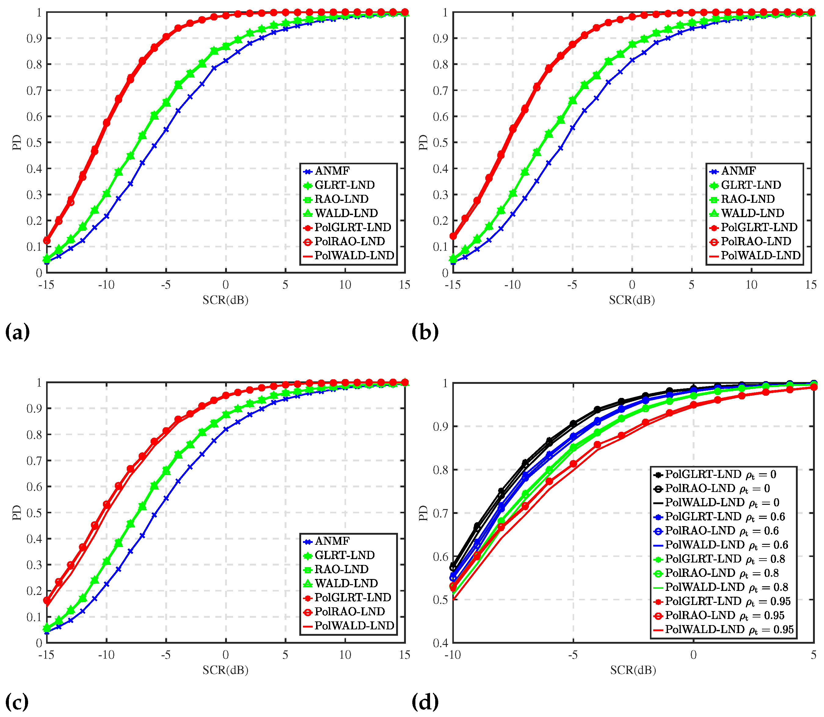
Figure 3 analyzes the impact of values of ${\rho }_{\mathrm{t}}$ on PD curves of all the detectors. The experimental setup includes $P_{\mathrm{FA}}={10}^{-4}$, $N=8$, $f_{\mathrm{d}}=0.3$, ${\alpha }_{\mathrm{pr}}=1$, known $\mathit{R}$, ${\lambda }_{\mathrm{HH}}={\lambda }_{\mathrm{HV}}=5$, ${\mu }_{\mathrm{HH}}={\mu }_{\mathrm{HV}}=1$, ${\rho }_{\mathrm{c}}=0$, and $\rho =0.9$. Figure 3a–c display the PD curves when ${\rho }_{\mathrm{t}}$ is set to 0, 0.6, and 0.95, respectively. As shown in these figures, the three proposed detectors exhibit similar performance and outperform the other detectors under the given simulation conditions. Figure 3d illustrates the PD curves for the three proposed detectors with ${\rho }_{\mathrm{t}}$ values of 0, 0.6, 0.8, and 0.95. As seen in Figure 3d, both of the proposed detectors’ detection performance decreases when ${\rho }_{\mathrm{t}}$ increases. This decline is due to the decreasing probability that the test statistics will surpass their respective detection thresholds as the correlation coefficient ${\rho }_{\mathrm{t}}$ rises.

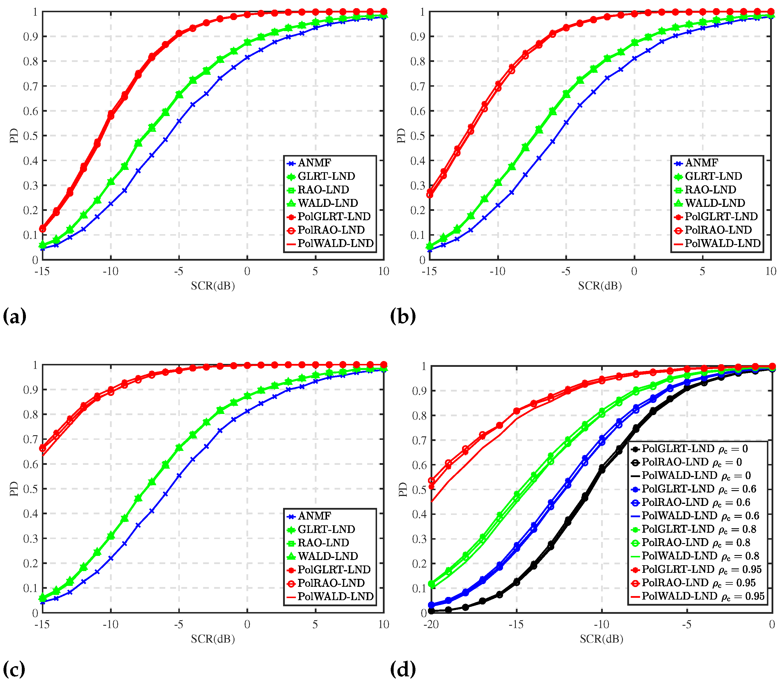
The impact of ${\rho }_{\mathrm{c}}$ values on PD curves for detectors is examined in Figure 4. The experimental parameters are set to $P_{\mathrm{FA}}={10}^{-4}$, $N=8$, $f_{\mathrm{d}}=0.3$, ${\alpha }_{\mathrm{pr}}=1$, with $\mathit{R}$ known, ${\lambda }_{\mathrm{HH}}={\lambda }_{\mathrm{HV}}=5$, ${\mu }_{\mathrm{HH}}={\mu }_{\mathrm{HV}}=1$, ${\rho }_{\mathrm{t}}=0$, and $\rho =0.9$. Figure 4a–c illustrate the PD curves against SCR for all detectors at ${\rho }_{\mathrm{c}}=0,0.6,0.95$, respectively. It is seen from Figure 4a–c that three proposed detectors outperform the competitors under the given simulation parameters, and that the performance gap widens with the increase in ${\rho }_{\mathrm{c}}$. Figure 4d presents the PD curves of the three proposed detectors for ${\rho }_{\mathrm{c}}=0,0.6,0.8,0.95$. Three proposed detectors exhibit improved detection performance with greater ${\rho }_{\mathrm{c}}$, as demonstrated in Figure 4d. This improvement is attributed to the whitening of correlated sea clutter.

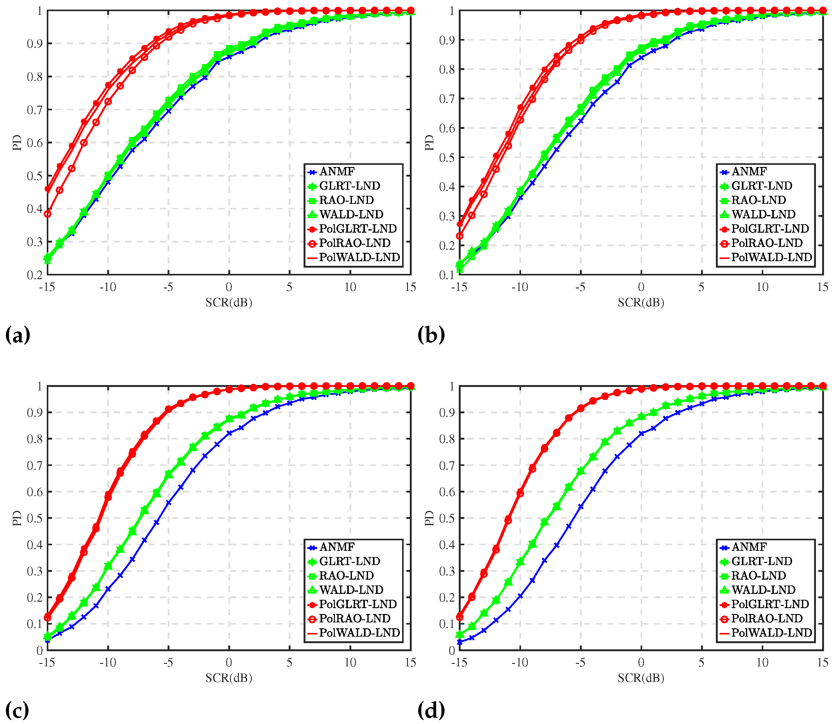
Figure 5 presents the PD curves for all detectors at various target average power ratios ${\alpha }_{\mathrm{pr}}$ and clutter average power ratios ${\mu }_{\mathrm{pr}}={\mu }_{\mathrm{HV}}/{\mu }_{\mathrm{HH}}$ between HV and HH polarimetric channels. The experimental parameters are set as $[{\alpha }_{\mathrm{pr}},{\mu }_{\mathrm{pr}}]=[[0.1,0.01],[0.1,0.05],[0.1,0.5],[0.1,1]]$, with ${\mu }_{\mathrm{HH}}=1$, $P_{\mathrm{FA}}={10}^{-4}$, $N=8$, $f_{\mathrm{d}}=0.3$, ${\rho }_{\mathrm{c}}=0$, $\mathit{R}$ known, ${\lambda }_{\mathrm{HH}}={\lambda }_{\mathrm{HV}}=5$, ${\rho }_{\mathrm{t}}=0$, and $\rho =0.9$. When ${\alpha }_{\mathrm{pr}}/{\mu }_{\mathrm{pr}}\ge 1$, the performance is evaluated using the SCR of the HV polarimetric channel; otherwise, the SCR of the HH polarimetric channel is used. Figure 5a–d demonstrate that the three proposed detectors outperform others under the given simulation parameters. This improved performance stems from the ability of the proposed detectors to leverage the polarimetric information from the channel with the smaller SCR, even when the performance evaluation is based on the maximum SCR between the HV and HH channels. Consequently, the enhancement in detector performance is directly related to the lower SCR.

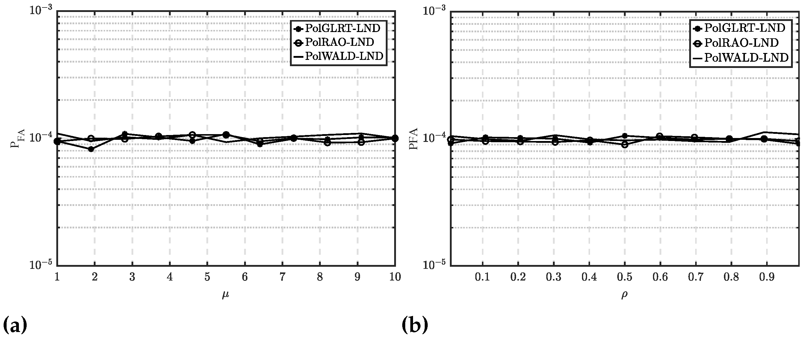
Figure 6 illustrates the $P_{\mathrm{FA}}$ curves for three proposed detectors with regard to $\mu$ and $\mathit{R}$. The experimental settings are $P_{\mathrm{FA}}={10}^{-4}$, $N=8$, $f_{\mathrm{d}}=0.3$, ${\rho }_{\mathrm{t}}=0$, ${\alpha }_{\mathrm{pr}}=1$, ${\lambda }_{\mathrm{HH}}={\lambda }_{\mathrm{HV}}=5$, $\mu ={\mu }_{\mathrm{HH}}={\mu }_{\mathrm{HV}}$, ${\mu }_{\mathrm{pr}}=1$, ${\rho }_{\mathrm{c}}=0$, and $\rho =0.9$. In Figure 6a, the $P_{\mathrm{FA}}$ is plotted against $\mu$ for $\mu$ values ranging from 1 to 10 with $\rho =0.9$. It shows that $P_{\mathrm{FA}}$ remains nearly unchanged as $\mu$ varies. Figure 6b depicts $P_{\mathrm{FA}}$ versus $\rho$ for $\rho$ values between 0.01 and 0.99 with $\mu$ set to 1. It reveals that variations in $\rho$ have minimal impact on $P_{\mathrm{FA}}$. Therefore, the simulations in Figure 6 confirm that three proposed detectors demonstrate an approximate CFAR property with respect to $\mu$ and $\mathit{R}$.

Figure 7 shows the clutter power map, amplitude fitting results, and the PD curves for all detectors. The 1998 IPIX dataset [39] was used to assess performance. The IPIX radar operates in dual linear polarization mode at a carrier frequency of 9.39 GHz, and the range resolution is 30 m. For the dataset 19980204_163113_ANTSTEP, the clutter texture parameters (${\widehat{\lambda }}_{\mathrm{HH}}$, ${\widehat{\lambda }}_{\mathrm{HV}}$, ${\widehat{\mu }}_{\mathrm{HH}}$, and ${\widehat{\mu }}_{\mathrm{HV}}$) were estimated using methods from [29,30] and integrated into the detectors. Experimental parameters were set as $P_{\mathrm{FA}}={10}^{-4}$, $N=8$, $f_{\mathrm{d}}=0.3$, ${\rho }_{\mathrm{t}}=0$, ${\widehat{\mu }}_{\mathrm{pr}}={\widehat{\mu }}_{\mathrm{HV}}/{\widehat{\mu }}_{\mathrm{HH}}$, ${\alpha }_{\mathrm{pr}}={\widehat{\mu }}_{\mathrm{pr}}$, and $L=26$. Simulated target signals were used to statistically calculate PD versus SCR. Figure 7a displays the clutter power map at HH and HV channels, revealing significant power fluctuations. Figure 7b–c present the fitting results for HH and HV polarization data, where the lognorm-texture CG distribution accurately models both the main and tail parts. Figure 7d indicates that the proposed PolGLRT-LND performs best, followed by PolWALD-LND. The performance advantage of PolRAO-LND is minimal. Due to the limited number of range cells (up to 26) in the measured radar data, accurately estimating the clutter speckle covariance matrix is challenging. A similar issue is evident in Figure 1a, implying that the proposed PolGLRT-LND and PolWALD-LND are more robust to clutter speckle covariance matrix estimation errors compared to PolRAO-LND.

5. Conclusions

This paper focused on polarimetric target detection in compound Gaussian sea clutter characterized by unknown covariance matrices and lognormal textures. We introduced three adaptive polarimetric coherent detectors utilizing two-step versions of GLRT, the Rao test, and Wald test. Experimental results demonstrate the superior performance of three proposed detectors. Incorporating texture distribution enables adaptation to varying degrees of non-Gaussian sea clutter, while dual-channel polarimetric information enhances target detection capabilities. Three designed detectors performs the approximate CFAR property with regard to speckle covariance matrices and scale parameters. Performance improvements are observed with increased secondary data quantity and clutter speckle correlation between polarimetric channels, as well as decreased target correlation between such channels. Although designed with two polarimetric channels, the detectors are easily adaptable to three or four channels. It is also necessary to emphasize that the three developed adaptive detectors improve clutter suppression and target detection performance by making use of polarization information, so they require the radar system to have a polarization mode of operation. The three proposed polarimetric adaptive coherent detectors work independently. However, joint detection using results from the three detectors may also be a viable method of enhancing performance. In future work, we will consider to jointly use the three detectors to improve the radar target detection performance.

References

1. Novak, L.M.; Burl, M.C.; Irving, W. Optimal polarimetric processing for enhanced target detection. IEEE Trans. Aerosp. Electron. Syst. 1993, 29, 234–244. [Google Scholar] [CrossRef]
2. Hao, C.; Gazor, S.; Ma, X.; Yan, S.; Hou, C.; Orlando, D. Polarimetric detection and range estimation of a point-like target. IEEE Trans. Aerosp. Electron. Syst. 2016, 52, 603–616. [Google Scholar] [CrossRef]
3. Lombardo, P.; Pastina, D.; Bucciarelli, T. Adaptive polarimetric target detection with coherent radar. II. Detection against non-Gaussian background. IEEE Trans. Aerosp. Electron. Syst. 2001, 37, 1207–1220. [Google Scholar] [CrossRef]
4. Barnard, T.J.; Weiner, D.D. Non-Gaussian clutter modeling with generalized spherically invariant random vectors. IEEE Trans. Signal Process. 1996, 44, 2384–2390. [Google Scholar] [CrossRef]
5. Ward, K. Compound representation of high resolution sea clutter. Electron. Lett. 1981, 16, 561–563. [Google Scholar] [CrossRef]
6. Weinberg, G.V. Assessing Pareto fit to high-resolution high-grazing-angle sea clutter. Electron. Lett. 2011, 47, 516–517. [Google Scholar] [CrossRef]
7. Mezache, A.; Soltani, F.; Sahed, M.; Chalabi, I. Model for non-Rayleigh clutter amplitudes using compound inverse Gaussian distribution: An experimental analysis. IEEE Trans. Aerosp. Electron. Syst. 2015, 51, 142–153. [Google Scholar] [CrossRef]
8. Carretero-Moya, J.; Gismero-Menoyo, J.; Blanco-del Campo, Á.; Asensio-Lopez, A. Statistical analysis of a high-resolution sea-clutter database. IEEE Trans. Geosci. Remote. Sens. 2009, 48, 2024–2037. [Google Scholar] [CrossRef]
9. Kelly, E.J. An adaptive detection algorithm. IEEE Trans. Aerosp. Electron. Syst. 1986, AES-22, 115–127. [Google Scholar] [CrossRef]
10. Robey, F.C.; Fuhrmann, D.R.; Kelly, E.J.; Nitzberg, R. A CFAR adaptive matched filter detector. IEEE Trans. Aerosp. Electron. Syst. 1992, 28, 208–216. [Google Scholar] [CrossRef]
11. De Maio, A. Rao test for adaptive detection in Gaussian interference with unknown covariance matrix. IEEE Trans. Signal Process. 2007, 55, 3577–3584. [Google Scholar] [CrossRef]
12. Conte, E.; Lops, M.; Ricci, G. Asymptotically optimum radar detection in compound-Gaussian clutter. IEEE Trans. Aerosp. Electron. Syst. 1995, 31, 617–625. [Google Scholar] [CrossRef]
13. Jay, E.; Ovarlez, J.P.; Declercq, D.; Duvaut, P. BORD: Bayesian optimum radar detector. Signal Process. 2003, 83, 1151–1162. [Google Scholar] [CrossRef]
14. Zhao, W.; Liu, C.; Liu, W.; Jin, M. Maximum eigenvalue-based target detection for the K-distributed clutter environment. IET Radar Sonar Navig. 2018, 12, 1294–1306. [Google Scholar] [CrossRef]
15. Shang, X.; Song, H.; Wang, Y.; Hao, C.; Lei, C. Adaptive detection of distributed targets in compound-Gaussian clutter with inverse gamma texture. Digit. Signal Process. 2012, 22, 1024–1030. [Google Scholar] [CrossRef]
16. Zhang, Y.C.; Shui, P.L. Antenna Beampattern Matched Optimum Coherent Detection in High-Resolution Mechanically Scanning Maritime Surveillance Radars. IEEE Trans. Aerosp. Electron. Syst. 2022, 59, 2764–2779. [Google Scholar] [CrossRef]
17. Zhang, X.J.; Shui, P.L.; Xue, Y.F. Long-time adaptive coherent detection of small targets in sea clutter by fast inversion algorithm of block tridiagonal speckle covariance matrices. Signal Process. 2024, 217, 109326. [Google Scholar] [CrossRef]
18. Wang, Z.; He, Z.; He, Q.; Li, J. Adaptive CFAR detectors for mismatched signal in compound Gaussian sea clutter with inverse Gaussian texture. IEEE Geosci. Remote. Sens. Lett. 2021, 19, 1–5. [Google Scholar] [CrossRef]
19. Wang, Z.; He, Z.; He, Q.; Cheng, Z. Persymmetric Range-Spread Targets Detection in Compound Gaussian Sea Clutter with Inverse Gaussian Texture. IEEE Geosci. Remote. Sens. Lett. 2022, 19, 8018305. [Google Scholar] [CrossRef]
20. Xue, J.; Liu, J.; Xu, S.; Pan, M. Adaptive detection of radar targets in heavy-tailed sea clutter with lognormal texture. IEEE Trans. Geosci. Remote. Sens. 2021, 60, 1–11. [Google Scholar] [CrossRef]
21. Pastina, D.; Lombardo, P.; Bucciarelli, T. Adaptive polarimetric target detection with coherent radar. I. Detection against Gaussian background. IEEE Trans. Aerosp. Electron. Syst. 2001, 37, 1194–1206. [Google Scholar] [CrossRef]
22. De Maio, A.; Alfano, G.; Conte, E. Polarization diversity detection in compound-Gaussian clutter. IEEE Trans. Aerosp. Electron. Syst. 2004, 40, 114–131. [Google Scholar] [CrossRef]
23. Alfano, G.; De Maio, A.; Conte, E. Polarization diversity detection of distributed targets in compound-Gaussian clutter. IEEE Trans. Aerosp. Electron. Syst. 2004, 40, 755–765. [Google Scholar] [CrossRef]
24. Kong, L.; Cui, G.; Yang, X.; Yang, J. Rao and Wald tests design of polarimetric multiple-input multiple-output radar in compound-Gaussian clutter. IET Signal Process. 2023, 20, 1–5. [Google Scholar] [CrossRef]
25. Shi, X.; Yang, C.; Wang, X.; Dong, S. Dual-Polarimetric Persymmetric Adaptive Subspace Detector for Range-Spread Targets in Heavy Tailed non-Gaussian Clutter. IEEE Geosci. Remote. Sens. Lett. 2023, 20, 85–96. [Google Scholar] [CrossRef]
26. Kang, N.; Huang, X.; Liu, W.; Liu, J.; Hao, C.; Shang, Z. Rao test of polarimetric detection for targets with energy spillover in non-Gaussian clutter. Digit. Signal Process. 2024, 144, 104266. [Google Scholar] [CrossRef]
27. Wang, J.; Wang, Z.; He, Z.; Li, J. GLRT-based polarimetric detection in compound-Gaussian sea clutter with inverse-Gaussian texture. IEEE Geosci. Remote. Sens. Lett. 2022, 19, 4028005. [Google Scholar] [CrossRef]
28. Wang, Z.; He, Z.; He, Q.; Xiong, B.; Cheng, Z. Polarimetric Target Detection in Compound Gaussian Sea Clutter with Inverse Gaussian Texture. IEEE Geosci. Remote. Sens. Lett. 2022, 19, 4021205. [Google Scholar] [CrossRef]
29. Chalabi, I.; Mezache, A. Estimators of compound Gaussian clutter with log-normal texture. Remote. Sens. Lett. 2019, 10, 709–716. [Google Scholar] [CrossRef]
30. Feng, T.; Shui, P.L. Outlier-robust tri-percentile parameter estimation of compound-Gaussian clutter with lognormal distributed texture. Digit. Signal Process. 2022, 120, 103307. [Google Scholar] [CrossRef]
31. Xue, J.; Ma, M.; Liu, J.; Pan, M.; Xu, S.; Fang, J. Wald-and Rao-based detection for maritime radar targets in sea clutter with lognormal texture. IEEE Trans. Geosci. Remote. Sens. 2022, 60, 1–9. [Google Scholar] [CrossRef]
32. Conte, E.; De Maio, A. Distributed target detection in compound-Gaussian noise with Rao and Wald tests. IEEE Trans. Aerosp. Electron. Syst. 2003, 39, 568–582. [Google Scholar] [CrossRef]
33. De Maio, A.; Iommelli, S. Coincidence of the Rao test, Wald test, and GLRT in partially homogeneous environment. IEEE Signal Process. Lett. 2008, 15, 385–388. [Google Scholar] [CrossRef]
34. Kay, S.; Zhu, Z. The complex parameter Rao test. IEEE Trans. Signal Process. 2016, 64, 6580–6588. [Google Scholar] [CrossRef]
35. Sun, M.; Liu, W.; Liu, J.; Hao, C. Complex parameter Rao, Wald, gradient, and Durbin tests for multichannel signal detection. IEEE Trans. Signal Process. 2021, 70, 117–131. [Google Scholar] [CrossRef]
36. Besson, O. Rao, Wald and Gradient Tests for Adaptive Detection of Swerling I Targets. IEEE Trans. Signal Process. 2023, 71, 3043–3052. [Google Scholar] [CrossRef]
37. Huang, C.; Wang, Y.L.; Liu, W.; Du, Q.; Liu, J. Adaptive double subspace target detection based on gradient test: Designs and comparisons. Digit. Signal Process. 2024, 145, 104323. [Google Scholar] [CrossRef]
38. Gini, F.; Greco, M. Covariance matrix estimation for CFAR detection in correlated heavy tailed clutter. Signal Process. 2002, 82, 1847–1859. [Google Scholar] [CrossRef]
39. Haykin, S. The McMaster IPIX Radar Sea Clutter Database. 1998. Available online: http://soma.ece.mcmaster.ca/ipix/ (accessed on 24 June 2024).
Figure 1. PD curves for P FA = 10 4 , N = 8 , f d = 0.3 , ρ t = 0 , α pr = 1 , λ HH = λ HV = 5 , μ HH = μ HV = 1 , ρ c = 0 and ρ = 0.9 . (a) L = 26 , (b) L = 32 , (c) L = 64 , (d) R is known.
Remotesensing 16 02841 g001
Figure 2. PD curves for P FA = 10 4 , N = 8 , f d = 0.3 , ρ t = 0 , α pr = 1 , R is known, μ HH = μ HV = 1 , ρ c = 0 and ρ = 0.9 . (a) λ = 0.5 , (b) λ = 1 , (c) λ = 5 , (d) λ = 10 .
Remotesensing 16 02841 g002
Figure 3. Influence of the value of ρ t on PD curves of detectors versus SCR for P FA = 10 4 , N = 8 , f d = 0.3 , α pr = 1 , R is known, λ HH = λ HV = 5 , μ HH = μ HV = 1 , ρ c = 0 and ρ = 0.9 . (a) ρ t = 0 , (b) ρ t = 0.6 , (c) ρ t = 0.95 . (d) Three proposed detectors with different values of ρ t .
Remotesensing 16 02841 g003
Figure 4. Influence of the value of ρ c on PD curves of detectors versus SCR for P FA = 10 4 , N = 8 , f d = 0.3 , α pr = 1 , R is known, λ HH = λ HV = 5 , μ HH = μ HV = 1 , ρ t = 0 and ρ = 0.9 . (a) ρ c = 0 , (b) ρ c = 0.6 , (c) ρ c = 0.95 . (d) Three proposed detectors with different values of ρ c .
Remotesensing 16 02841 g004
Figure 5. PD curves for P FA = 10 4 , N = 8 , f d = 0.3 , R is known, λ HH = λ HV = 5 , μ HH = 1 , ρ t = 0 and ρ = 0.9 . (a) α pr = 0.1 , μ pr = 0.01 , (b) α pr = 0.1 , μ pr = 0.05 , (c) α pr = 0.1 , μ pr = 0.5 , (d) α pr = 0.1 , μ pr = 1 .
Remotesensing 16 02841 g005
Figure 6. P FA curves for P FA = 10 3 , N = 8 , f d = 0.3 , ρ t = 0 , α pr = 1 , λ HH = λ HV = 5 , μ = μ HH = μ HV , μ pr = 1 , ρ c = 0 and ρ = 0.9 . (a) PFA versus μ for ρ = 0.9 . (b) PFA versus ρ for μ = 1 .
Remotesensing 16 02841 g006
Figure 7. Power map, amplitude fitting results, and PD curves when using 19980204_163113_ANTSTEP. (a) Sea clutter power map. (b) Amplitude fitting result of HH data. (c) Amplitude fitting result of HV data. (d) L = 26 .
Remotesensing 16 02841 g007
Disclaimer/Publisher’s Note: The statements, opinions and data contained in all publications are solely those of the individual author(s) and contributor(s) and not of MDPI and/or the editor(s). MDPI and/or the editor(s) disclaim responsibility for any injury to people or property resulting from any ideas, methods, instructions or products referred to in the content.