Technical Note

Angle Estimation Using Learning-Based Doppler Deconvolution in Beamspace with Forward-Looking Radar

1
National Key Laboratory of Microwave Imaging, Aerospace Information Research Institute, Chinese Academy of Sciences, Beijing 100190, China
2
School of Electronic, Electrical and Communication Engineering, University of Chinese Academy of Sciences, Beijing 100049, China
3
The 27th Research Institute of China Electronics Technology Group Corporation, Zhengzhou 450047, China
*
Author to whom correspondence should be addressed.
Remote Sens. 2024, 16(15), 2840; https://doi.org/10.3390/rs16152840
Submission received: 7 July 2024 / Revised: 29 July 2024 / Accepted: 31 July 2024 / Published: 2 August 2024

Abstract

:
The measurement of the target azimuth angle using forward-looking radar (FLR) is widely applied in unmanned systems, such as obstacle avoidance and tracking applications. This paper proposes a semi-supervised support vector regression (SVR) method to solve the problem of small sample learning of the target angle with FLR. This method utilizes function approximation to solve the problem of estimating the target angle. First, SVR is used to construct the function mapping relationship between the echo and the target angle in beamspace. Next, by adding manifold constraints to the loss function, supervised learning is extended to semi-supervised learning, aiming to improve the small sample adaptation ability. This framework supports updating the angle estimating function with continuously increasing unlabeled samples during the FLR scanning process. The numerical simulation results show that the new technology has better performance than model-based methods and fully supervised methods, especially under limited conditions such as signal-to-noise ratio and number of training samples.

1. Introduction

Forward-looking radar (FLR) is attracting significant attention due to its capability to operate under various weather conditions and throughout the day. This has generated considerable interest in the research and development of FLR technologies, particularly for applications in aircraft navigation, enemy detection, surveillance, and missile guidance [1,2,3]. Given its extensive range, even a slight deviation in the azimuth angle can lead to a significant error in target positioning. In FLR, achieving high-accuracy range positioning requires the use of wide-bandwidth signals, while improving azimuth positioning accuracy can be achieved by increasing the radar’s physical aperture size. Additionally, a high signal-to-noise ratio (SNR) is crucial for the system’s performance.
Under the constraint of the limited azimuthal aperture of the antenna, antenna pattern deconvolution [4] (APD) technology has been widely used in forward-looking detection to improve positioning accuracy. APD technology employs the overlap scanning of antenna beams to establish an observation model [5], and spectral estimation [2,4,5,6,7,8] and the Bayesian method [1,3,9,10,11,12] are introduced to solve the model in FLR imaging to achieve super-resolution imaging. Considering the combined utilization of antenna pattern and Doppler information generated by high-speed platform motion, a Bayesian forward-looking imaging model [1] is employed to explore the sparse structure of the target, significantly improving imaging resolution. However, these methods rely on certain prior information, such as the antenna pattern and the relative velocity of the target to the platform. The model-based methods mentioned above divide the space into discrete grids and estimate the target intensity on each grid, so that off-grid [13,14,15] phenomena can lead to positioning errors. Moreover, most of the algorithms proposed in these references are geared towards high-resolution imaging applications. The majority of these methods require iterative optimization, leading to efficiency issues. However, real-time processing is a pressing need for high-precision target localization.
In recent years, machine learning methods such as neural networks [16,17,18,19,20,21,22] and support vector machines [23,24,25,26,27,28,29,30] (SVMs) have become powerful tools in array signal processing (ASP) due to their nonlinear properties and generalization capability, etc. To the best of our knowledge, most of the present work focuses on digital array systems. Phased array FLR, which uses analog phase shifters for beamforming, has lower cost and system complexity and is more widely used. Therefore, adopting a learning-based approach for FLR target angle estimation is of great research value. However, it is difficult to establish a large enough training dataset to cover the distribution of all test data due to the existence of a large number of parameters in FLR, such as platform speed, SNR, and noise samples. As a result, in spite of the above great achievements, there are still many problems to be addressed further in FLR high-precision target positioning applications.
Motivated by the above, this paper proposes a semi-supervised learning framework for FLR angle estimation (SSL-FAE), which considers FLR target angle estimation as a function approximation problem. Firstly, support vector regression (SVR) is used to establish the mapping relationship between the gain of FLR beam scanning and Doppler phase variation, which is named Doppler deconvolution [1]. Secondly, by adding manifold regularization [31] to the loss function, supervised learning is extended to semi-supervised learning, improving the small sample adaptation ability. In practical situations, the parameters of the target and the platform are often coupled and complex to model, usually requiring extensive preprocessing work. This paper employs machine learning to directly fit the target’s position. By avoiding numerous intermediate steps and modeling errors caused by manual modeling, this approach significantly enhances the accuracy of estimation. Furthermore, the model-based algorithms typically treat the target localization problem as a classification task. In contrast, the method proposed in this paper treats it as a regression problem, thereby avoiding errors caused by off-grid effects.
Compared with existing methods, this article has the following innovations:
  • An end-to-end learning-based FLR target angle estimation framework is established, which omits the computationally expensive iterative optimization.
  • A regression strategy is adopted, which can avoid the off-grid effects.
  • A semi-supervised mechanism is introduced in learning through the manifold regularization framework to avoid building overly large FLR target positioning datasets.

2. Methods

2.1. Mathematical Model

The geometric model for the moving platform FLR is shown in Figure 1. In the coordinate defined by O x y z , the platform flies along the X-direction with a constant velocity, v, at altitude H. R 0 is the initial range between the radar and the point target, P. R ( t ) is the range of the radar to the target at the slow time, t. θ and φ denote initial azimuth and elevation angles. It is assumed that the linear frequency modulation (LFM) signal is transmitted through the phased array FLR, as indicated in Equation (1).
s ( τ ) = r e c t ( τ T ) × exp j 2 π ( f c τ + K r 2 τ 2 )
where r e c t ( · ) represents the unit rectangular window signal, f c denotes the center frequency of the LFM signal, K r represents the frequency modulation slope, and τ and T represent fast time and transmitted pulsewidth, respectively. At a particular slow time, t, the phased array beam is directed towards θ t . The echo signal can be represented as the sum of the reflected waves from all targets, and its specific form is shown in Equation (2).
s r ( t , τ ) = i N P σ ( R ( t ) , θ ) · h θ θ t × exp j 2 π f d t × sinc B w τ 2 R ( t ) c exp j 4 π R 0 λ
where N P is defined as the number of targets, σ r , θ represents the reflection coefficient function of a point target, h ( · ) represents the two-way antenna pattern function, λ and B w denote the wavelength and the bandwidth of the LFM signal, and c represents the speed of light. f d is the Doppler frequency caused by the movement of the platform, which can be expressed as
f d = 2 v λ cos θ ( t ) cos φ
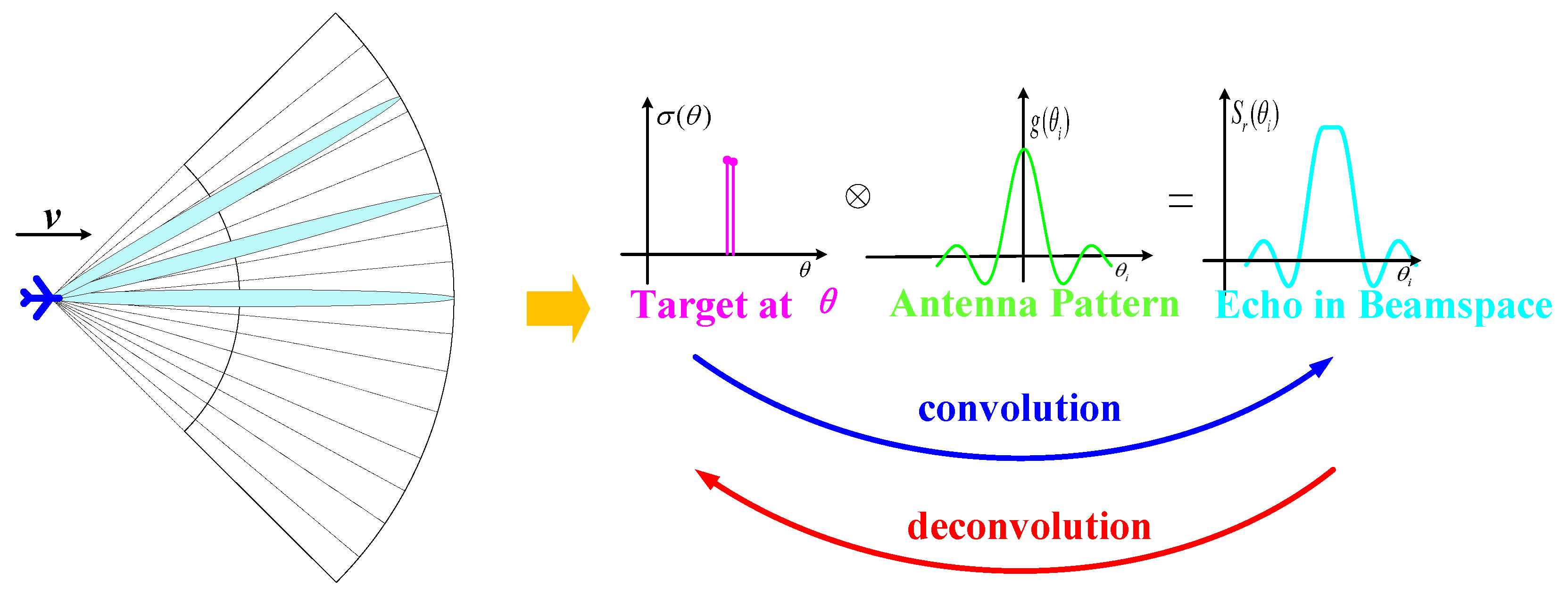
In Equation (2), the function sinc ( · ) is defined by s i n c ( x ) = s i n ( π x ) / ( π x ) , which represents the envelope of the range point spread function. Given the high pulse repetition frequency (PRF) of the radar, it is presumed that the range migration (RM) of the target does not exceed the range resolution unit. Further, on high-speed platforms, the RM of more than one resolution unit can be corrected using the keystone transform [32]. Referring to Equation (2), it is evident that echo signals from various beam-scanning angles within the same distance resolution unit can be treated as the convolution of the reflection coefficient and the product of the Doppler phase and antenna pattern, as shown in Figure 2.
In the scenario of phased-array scanning, a total of M samples of azimuth scanning grid are acquired, denoted as θ i , i = 1 , , M . The echo data corresponding to the ith scanning angle at a specific range cell are represented as s r θ i . The signal vector for the echo data is denoted as Equation (4).
S = s r θ 1 , s r θ 2 , , s r θ M T
The task of FLR angle estimation involves determining the true angle, θ m i n ( θ i ) , m a x ( θ i ) , of the target based on the vector S . The well-known approach is to treat this problem as a classification issue, assuming the existence of N possible true angles, i.e., Θ = θ ^ i , i = 1 , , N . In general, θ ^ i is evenly distributed between m i n ( θ i ) and m a x ( θ i ) . Let Σ denote the unknown scattering coefficient vector of the target, as depicted in Equation (5).
Σ = σ 1 , σ 2 , , σ N T
where, σ i denotes the scattering coefficient of the target in θ ^ i . To determine the true angles of the targets, it is necessary to estimate Σ based on the known S , and then perform peak searching on Σ . To ensure that the true angles of the targets are included in Θ , the grid division of Θ needs to be sufficiently dense, i.e., N > > M .
Next, it is necessary to establish the mapping relationship from S to Σ . According to Equation (2), the Doppler deconvolution model can be linearly expressed as
S = H D Σ + G
where ⊙ denotes the Hadamard product. Considering that white noise is generally adopted in typical FLR studies [1,33,34], Gaussian white noise represented by G is added to the signal. H represents antenna pattern information, and its specific form is shown in Equation (7).
H = h 11 h 12 h 1 N h 21 h 22 h 2 N h M 1 h M 2 h M N
In Equation (7), h i j = h ( θ i θ j ) represents the product of the directional two-way antenna pattern gain of the ith sample of the azimuth scanning angle, θ i , the jth possible true angle, θ j . D represents the Doppler matrix, as shown in Equation (8).
D = e j π 2 f d 1 P R F e j π 2 f d 2 P R F e j π 2 f d N P R F e j π 4 f d 1 P R F e j π 4 f d 2 P R F e j π 4 f d N P R F e j π 2 M f d 1 P R F e j π 2 M f d 2 P R F e j π 2 M f d N P R F
In Equation (8), f d i represents the Doppler frequency of the ith sample of the azimuth scanning angle, which can be expressed as
f d i = 2 v λ cos θ ^ i cos φ
By establishing a discrete linear model based on Equation (6), existing model-based approaches such as the minimum variance distortionless response [35] (MVDR), compressive sensing [36] (CS), etc., can be employed, which enables the calculation of the target scattering coefficient vector, Σ . For example, within the compressive sensing framework, Σ can be obtained by solving Equation (10).
Σ = arg min S H D Σ 2 2 + γ Σ 1
where γ denotes the regularization coefficient. Furthermore, by performing a peak search on Σ , the target angle can be determined.
In the SSL framework, the task of FLR angle estimation is to establish a direct mapping relationship from vector S to the target azimuth angle, θ . As radar data typically include both amplitude and phase, S is a complex vector. After normalizing vector S , the real-valued processing is performed, as shown in Equation (11).
Z = real S T , imag S T T S
Furthermore, the task of the learning framework is transformed into a mapping from vector Z to the target angle, θ . That is, a certain transformation is applied to vector Z through the function g ( · ) , aiming to make the transformed output, g ( Z ) , as close as possible to the target angle, θ . If given a set of labeled data Z ¯ i , θ ¯ i , i = 1 , , L , within the SVR framework, the corresponding loss function is formulated in the form of Equation (12).
g * = arg min g i ( g ( Z ¯ i ) θ ¯ i ) 2 + λ g 2
where · 2 represents the L 2 norm, used to prevent overfitting. To employ a semi-supervised strategy in Equation (12), manifold regularization is contemplated. Assuming that all labeled and unlabeled data lie on a low-dimensional manifold, if two input samples are proximate in this structure, their output results should also be proximate. Specifically, influenced by factors such as direction diagram errors, motion errors, and noise, the output features of the array radar, represented by Z in the original space, may not be uniform. However, they are expected to be constrained within a certain manifold space, M . In other words, within M , if the distance between the features Z ¯ i and Z ¯ j from the array output is sufficiently small, then the corresponding target angles, θ ¯ i and θ ¯ j , should also be proximate. Based on this characteristic, if given a set of unlabeled data Z ¯ i , i = L + 1 , , P , combined with Equation (12), the objective function for optimization can be expressed as [31,37]
g * = arg min g H i = 1 L g Z ¯ i θ ¯ i 2 + λ H g H 2 + 1 2 λ M i , j = 1 P W i j g Z ¯ i g Z ¯ j 2
where i = 1 L g Z ¯ i θ ¯ i 2 represents empirical risk, indicating the closeness between labeled angle estimation results and label values after the action of function g ( · ) , utilizing information from all labeled data. g H 2 is the norm defined in the reproducing kernel Hilbert space [38,39] (RKHS), used to prevent overfitting. i , j = 1 P W i j g Z ¯ i g Z ¯ j 2 expresses the manifold structure in M , where W i j is the weight parameter representing the similarity in the manifold, M , between Z ¯ i and Z ¯ j (including labeled and unlabeled data). This is to achieve semi-supervised learning, and W i j is typically expressed as the radial basis function [23] (RBF).
W i j = exp Z ¯ i Z ¯ j 2 η M
where, η M is the Gaussian bandwidth parameter. It can be observed that, as the distance between Z ¯ i and Z ¯ j decreases, the value of W i j increases, thereby imposing constraints on g ( · ) to ensure the estimated angle values are closely approximated. Typically, only a finite number of nearest neighbors are considered, i.e., only sufficiently large finite W i j are selected, while the others are set to zero.

2.2. Angle Estimation Using SSL-FAE

According to Equation (13) and the representation theorem [40], it is evident that, given the test data, Z , the expression for estimating θ ^ is represented as:
θ ^ = g * ( Z ) = i = 1 P β i κ Z ¯ i , Z
where κ adopts RBF with the bandwidth parameter η H , which can be expressed as
κ Z i , Z j = exp Z i Z j 2 η H
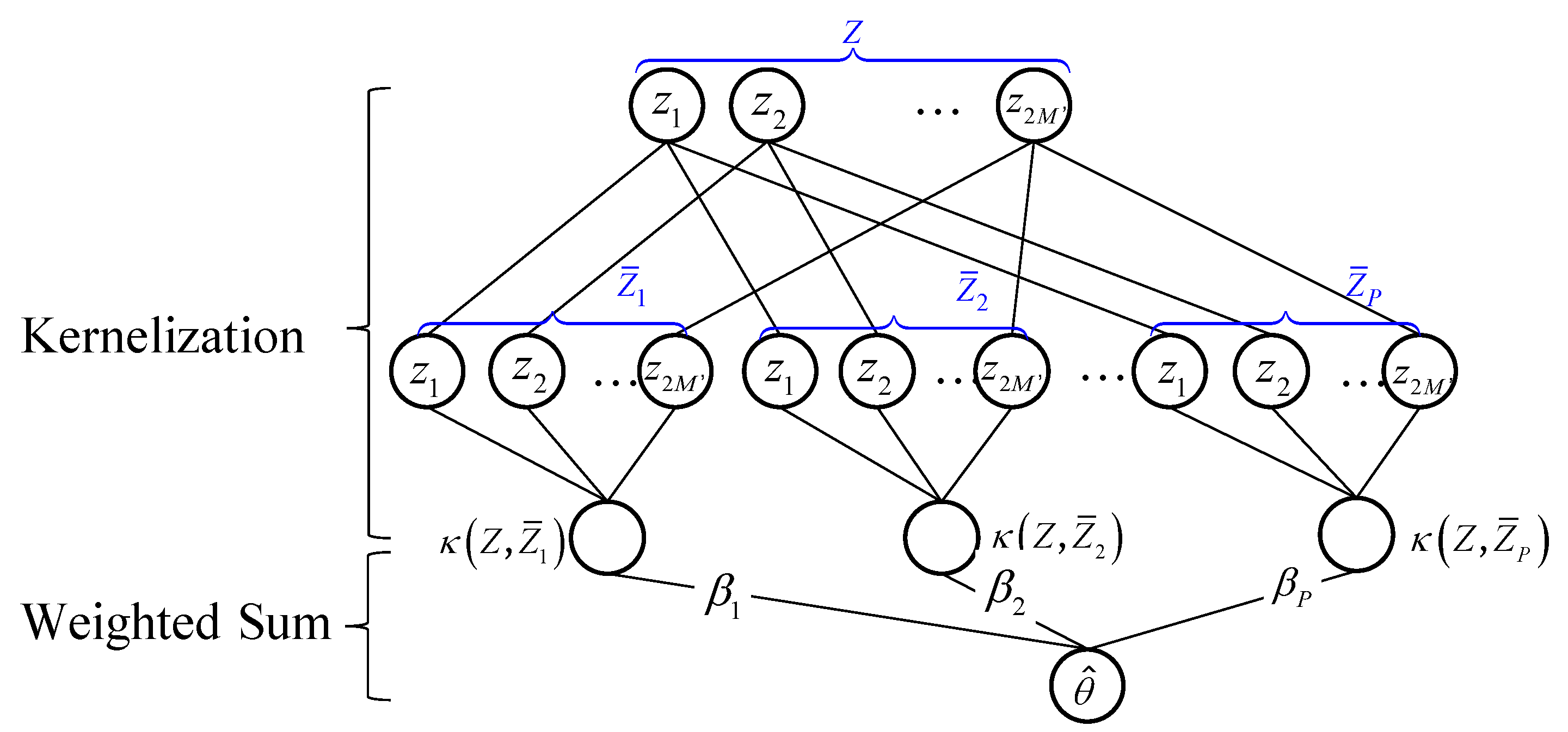
The azimuth of the target is expressed as a linear combination of the kernel functions, where B = β 1 , , β P represents the coefficients of the combination. The estimation process of the SSL-FAE is illustrated in Figure 3, and it consists of two stages: kernelization and weighted summation. In the kernelization stage, the correlation matrix of the test samples is connected with the correlation matrix of all training samples, establishing the RBF. By linearly combining these RBFs, the target angle can be estimated.

2.3. Training SSL-FAE

The crucial aspect of model training is obtaining the vector, B , of combination coefficients based on Equation (13). In Equation (13), g H 2 denotes the norm of the function g ( · ) defined in the RKHS. In accordance with the property of the reproducing kernel, it can be expressed as
g H 2 = i j β i β j κ Z ¯ i , Z ¯ j = B T K B
where K R P × P is a square matrix composed of the kernel function κ Z i , Z j .
In Equation (13), i , j = 1 P W i j g Z ¯ i g Z ¯ j 2 expresses the manifold structure in M , which can be expressed in detail as [31,37]
i , j = 1 P W i j g Z ¯ i g Z ¯ j 2 = i = 1 P g Z ¯ i 2 j = 1 P W i j i = 1 P j = 1 P g Z ¯ i g Z ¯ j W i j = i = 1 P g Z ¯ i 2 j = 1 P W i j W i i i = 1 P j = 1 , j i P g Z ¯ i g Z ¯ j W i j
Consider expressing Equation (18) in matrix form. Let D i = j = 1 P W i j and D = d i a g D 1 , D 2 , , D P . W is an affinity matrix formed by W i j . The notation is defined as L = W D , where L represents the Laplacian matrix. Thus,
i , j P W i j g Z ¯ i g Z ¯ j 2 = i P g Z ¯ i 2 D W i i i P j , j i P g Z ¯ i g Z ¯ j W i j = i P j P g Z ¯ i L i j g Z ¯ j = B T K L K B
In Equation (13), i = 1 L g Z ¯ i θ ¯ i 2 represents empirical risk, and it can be expressed as
i = 1 L g Z ¯ i θ ¯ i 2 = i = 1 L B T K ( : , i ) θ ¯ i 2 = ( J KB Θ ) T ( J KB Θ )
where
Θ = [ θ 1 , θ L L , 0 , , 0 P L ] T J = diag { 1 , 1 L , 0 , , 0 P L }
After the matrixization process, substituting Equations (17), (19), and (20) into Equation (13), the objective function for optimization can be rewritten as
B * = arg min g H ( J KB Θ ) T ( J KB Θ ) + λ H B T KB + 1 2 λ M B T K L KB
Since Equation (22) is a second-order polynomial about the combination coefficient vector, B , it has an explicit solution. Setting its derivative with respect to B to zero allows us to obtain the solution for B , which can be given as [31]
B * = λ H I P + 1 2 λ M L K + J K 1 J Θ
where I P represents the Pth-order identity matrix.

3. Numerical Simulations and Results

A uniform phased array consisting of 60 antenna elements spaced at half-wavelength intervals is considered to verify the performance of the proposed method. The specific simulation parameters are as Table 1.
This paper compares the SSL-FAE with two previously existing classic model-based estimation architectures. One only considers antenna pattern information [2,3,6,7,8]. The other approach considers the Doppler information generated by platform motion based on the antenna pattern [1]. The MVDA and Bayesian [1] methods are utilized to solve the above two models, respectively. Furthermore, the SSL-FAE is compared with SVR to demonstrate their performance. The parameters used for the SSL-FAE during training and testing are shown in Table 2.
In the training stage, the labeled training azimuth angle set is uniformly scanned from 10 to 10 , encompassing a total of 150 beams, while the unlabeled training azimuth angle set is uniformly scanned from 10 to 10 , encompassing a total of 1500 beams. The speed of the platform is randomly generated within the range 0 to 250 km/h.

3.1. Experiment 1

3.1.1. Case 1

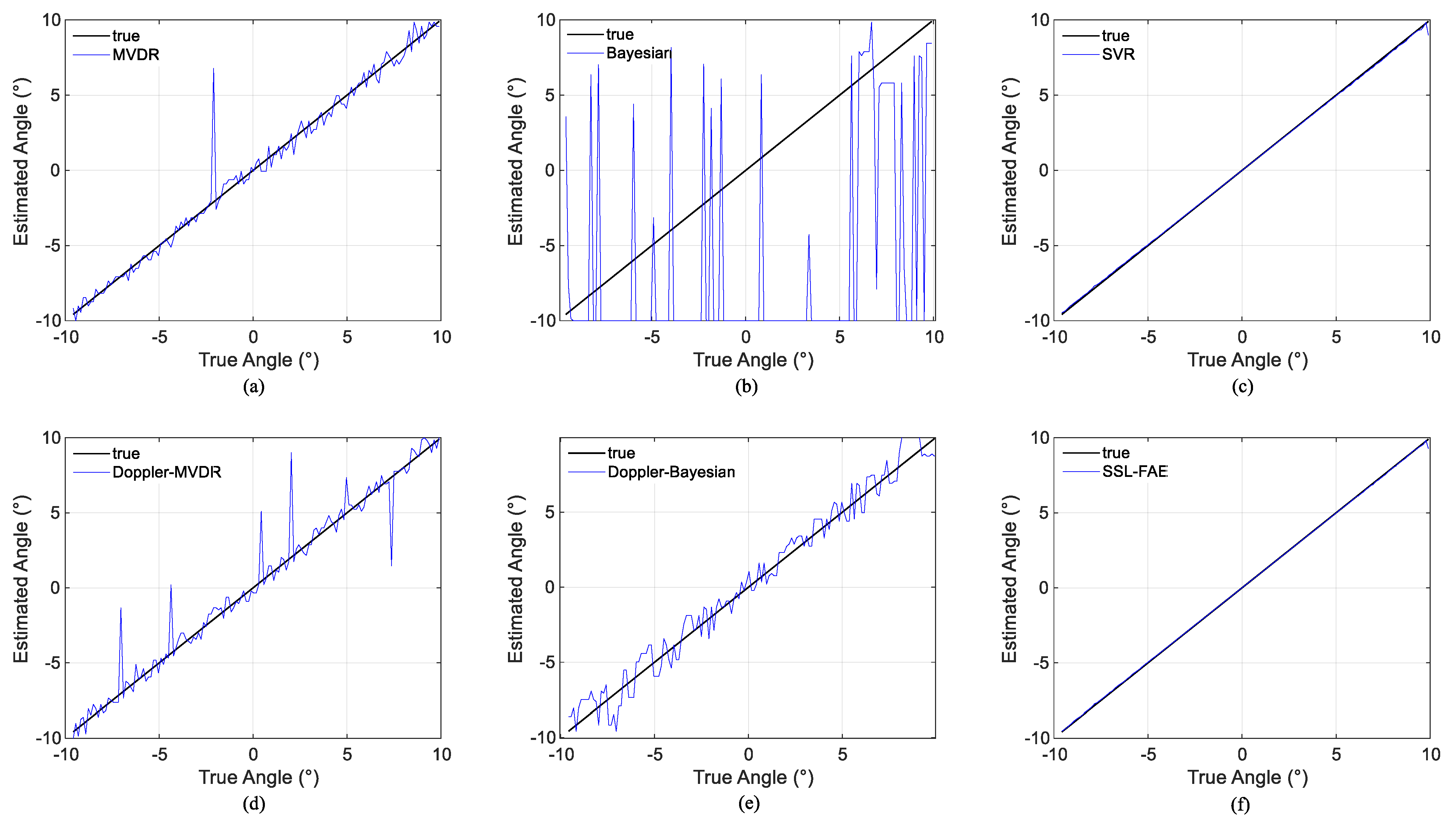
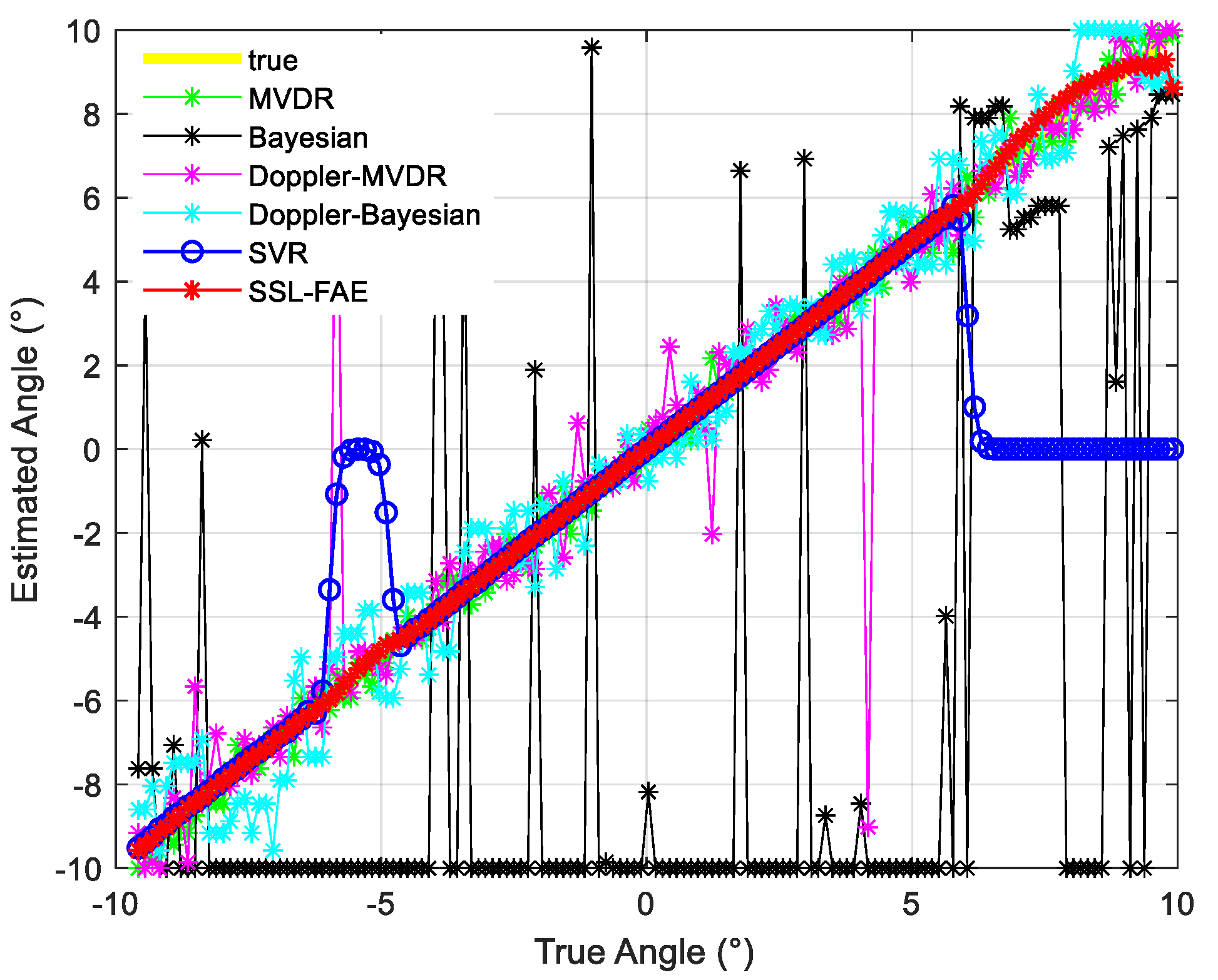
To evaluate the effectiveness of the proposed method, the first simulation considers a single target from different angles. In this simulation, 150 azimuth angles are chosen randomly within 10 , 10 (not included in the training set) to form the test azimuth angle set. The MVDR, Doppler–MVDR, Bayesian, Doppler–Bayesian, SVR, and SSL-FAE methods are utilized for testing, as shown in Figure 4.
In Figure 4, the horizontal axis represents the true values, while the vertical axis represents the estimated values of each algorithm. Ideally, if the estimation results are entirely accurate, they will align along a straight line with a slope of 1. Figure 4a,b demonstrate that, under the conventional deconvolution model, estimating the azimuth angle of the point target is challenging when the platform is running at high speed. In Figure 4d,e, it is clear that the Doppler–Bayesian deconvolution model can suppress the noise amplification. However, the estimated results are still experiencing fluctuations relative to the true values. Figure 4c,f reveal that both the SVR method and the SSL-FAE perform significantly well, which can be attributed to the labeled training set covering angles from 10 to 10 .

3.1.2. Case 2

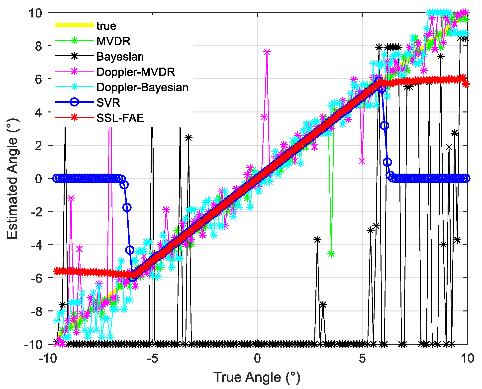
To investigate the semi-supervised performance of manifold regularization, the number of labeled samples in the training set is reduced. To further investigate, building upon Case 2, the labeled samples in the range from 6 to 10 are removed from the training set, and a new round of testing is conducted, as shown in Figure 5. The experimental results demonstrate that, in regions where labeled data are absent, the fully supervised SVR method fails to accurately estimate the angles of the targets. In contrast, the SSL-FAE proposed in this paper effectively leverages the interplay between labeled and unlabeled information through manifold regularization. As a result, even in areas with missing labeled information, the SSL-FAE exhibits strong performance and is able to provide accurate estimations.

3.1.3. Case 3

In order to investigate the mechanism of semi-supervised learning, the amount of labeled data in the training set are further reduced. Building upon previous experiments, the labeled training samples within the symmetric region 10 to 6 are further reduced. The results of this experiment are depicted in Figure 6. When the labeled training data are lacking in the symmetric region, the SSL-FAE exhibits a certain degree of failure in estimating this particular region. This suggests that the semi-supervised functionality of manifold regularization is achieved by leveraging the labeled samples from the symmetric region, as the antenna’s radiation pattern also exhibits symmetric variations during beam scanning.

3.1.4. Case 4

To validate the aforementioned hypothesis, building upon the experiment in Case 2, the labeled training data within the target angle ranging from 6 to 5.5 are further reduced. The new experimental results are illustrated in Figure 7. It can be inferred that SVR has become ineffective in regions lacking labeled data supervision, specifically within the ranges 6 to 5.5 and 6 to 10 . However, since there exist labeled data in their symmetric regions, i.e., 10 to 6 and 5.5 to 6 , the SSL-FAE uses manifold regularization to establish correlation constraints between unlabeled data and the labeled data of symmetric regions.

3.1.5. Case 5

This section further discusses the case where there is no post-symmetry overlap of labeled samples. Building on Case 4, the labeled training samples within the region from 8.7 to 6 are further reduced, i.e., there are no labeled samples in the symmetric portion 6 to 8.7 . The results in Figure 8 indicate that the SSL-FAE can still accurately estimate the angle of the target located in the regions from 8.7 to 6 and their symmetric regions. The semi-supervised effect of manifold regularization remains effective, even when some samples from the symmetric regions are missing. This is because the Doppler effect caused by the movement of the platform and target contains information about the target’s position, combined with the symmetric nature of the antenna radiation pattern. Nevertheless, compared with the results in Figure 7, the estimation accuracy in the areas without samples shows a significant decline.
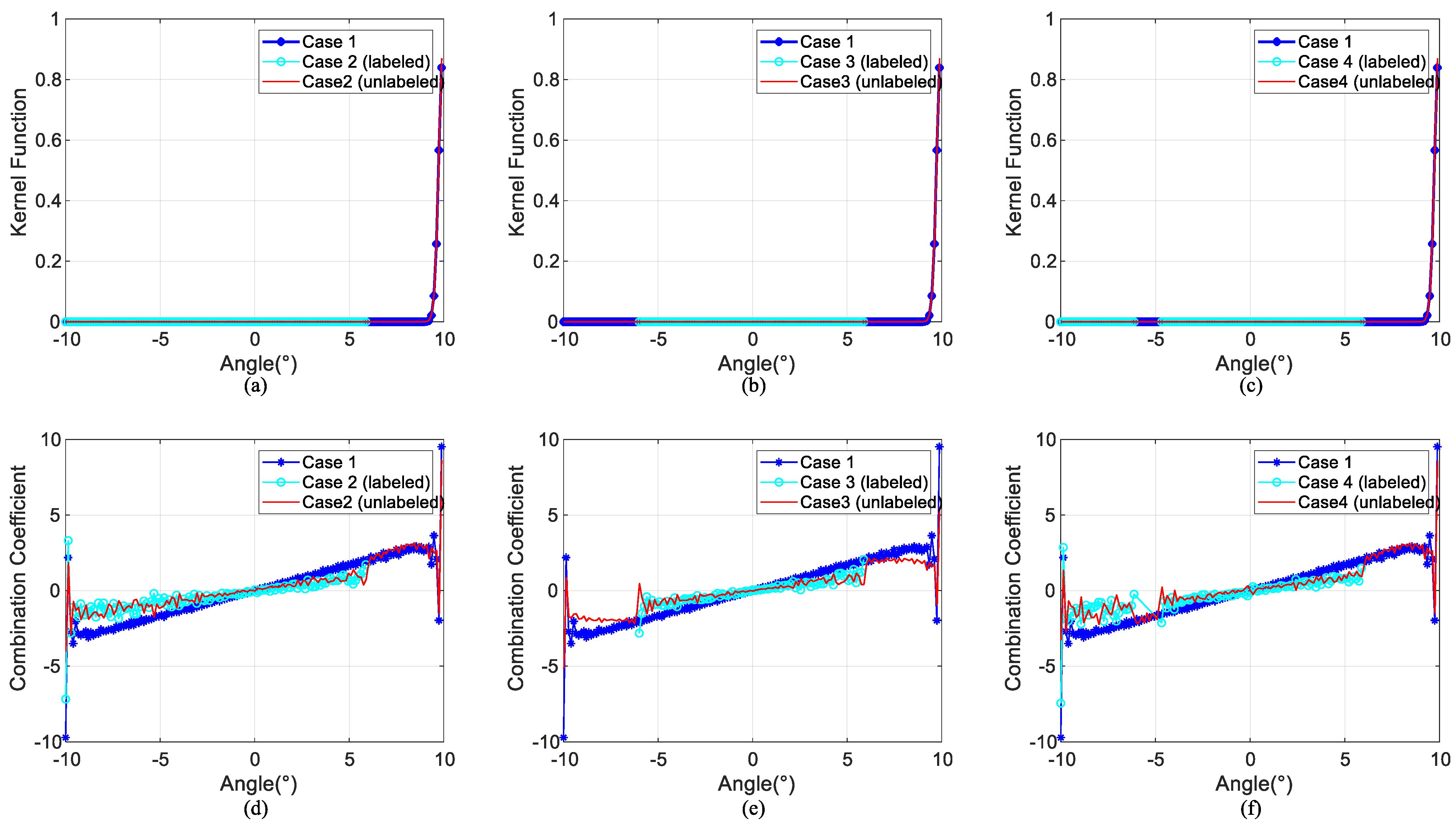
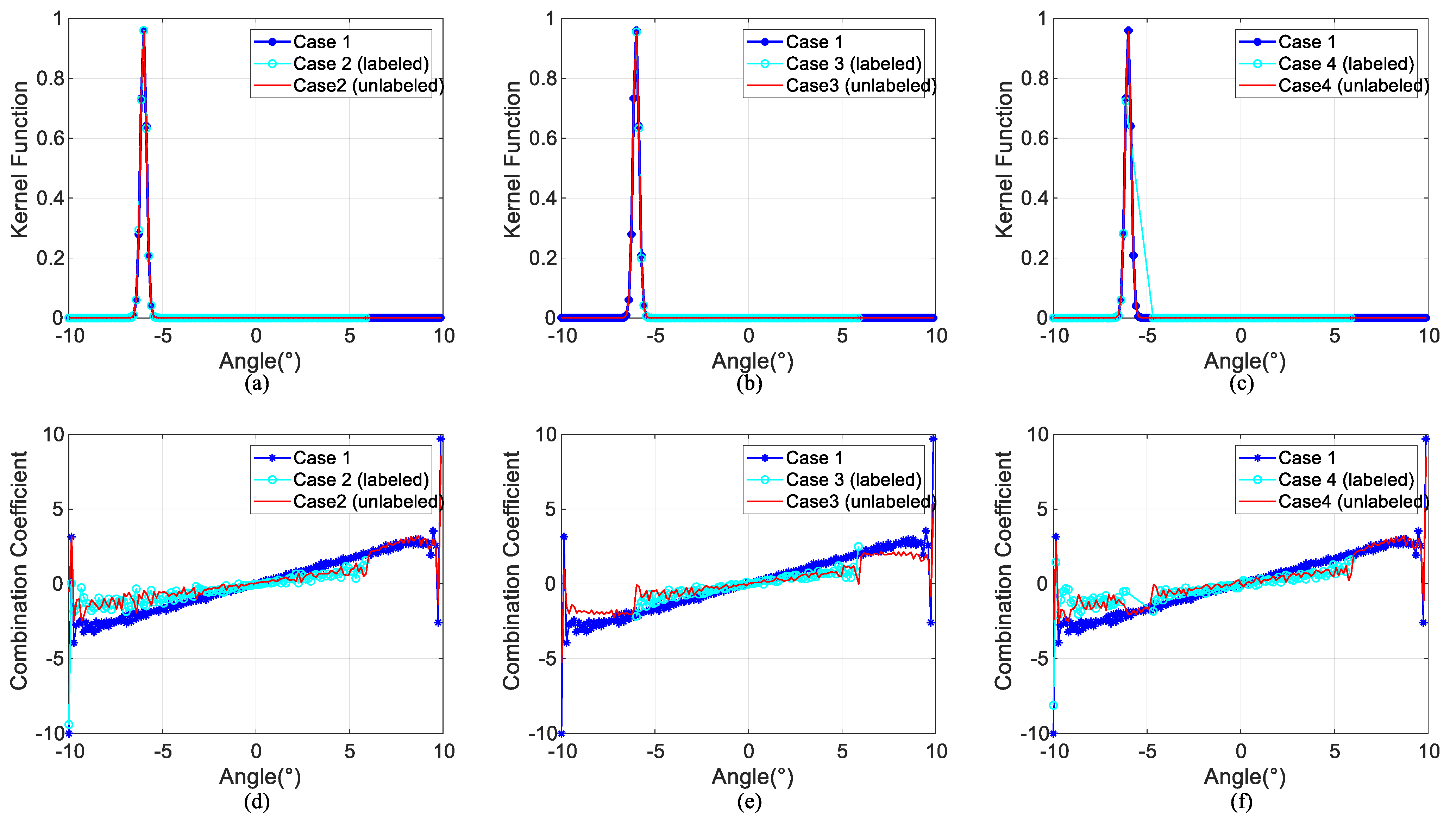
To discuss the role of manifold regularization in the SSL-FAE, we analyzed the values of the kernel function and the combination coefficient in Cases 1–4. Figure 9 and Figure 10 illustrate the scenarios when the target is at 5.3 and 10 , respectively. In Figure 9a–c, it can be seen that, in the regions corresponding to labeled data, several kernel functions, κ , near 10 exhibit significant increases, while other areas remain unchanged. Since the training samples in Case 1 cover the range from 10 to 10 , this region can serve as a benchmark for quantifying semi-supervised capability. In Figure 9d,e, it is evident that the combination coefficients, β , in the region without labeled samples deviate from the Case 1 situation. However, due to the presence of labeled samples in the symmetrical region, the unlabeled samples still align with the Case 1 situation, as shown in Figure 9f. This indicates that, even if the actual angular position of the target does not have labeled samples, as long as there are labeled samples in its symmetrical region, the SSL-FAE can still be effective. In Figure 10, due to the change in the position of the test target, the peak positions of the kernel functions also change. This indicates that the working mechanism of the SSL-FAE involves first determining the approximate position of the target by expressing the correlation between the actual data and the samples through the kernel functions, and then further fitting the target’s true angle through the combination coefficients.

3.2. Experiment 2

In this experiment, the statistical performance of the MVDR, Bayesian, Doppler–MVDR, Doppler–Bayesian, SVR, and SSL-FAE under different SNRs are considered. The training set used is the same as in Experiment 1. In this experiment, Gaussian white noise at different power levels is added after pulse compression. The test set consists of target angles located in regions with labeled test samples. Additionally, the corresponding SNR matching the training samples is added to the test samples. The results of the experiment are as shown in Figure 11, and root mean squared error (RMSE) is utilized to evaluate the statistical performance of different methods.
The results indicate that the Doppler–Bayesian method has higher accuracy compared with other methods, as it partially corrects Doppler errors caused by platform motion and mitigates overfitting through regularization. Nevertheless, it does not account for Doppler errors induced by high-speed target movement. Therefore, its estimation performance cannot be effectively utilized. However, SVR and the SSL-FAE demonstrate superior performance in high-precision localization of moving targets by extensively incorporating targets with unknown speeds into their model training.

3.3. Experiment 3

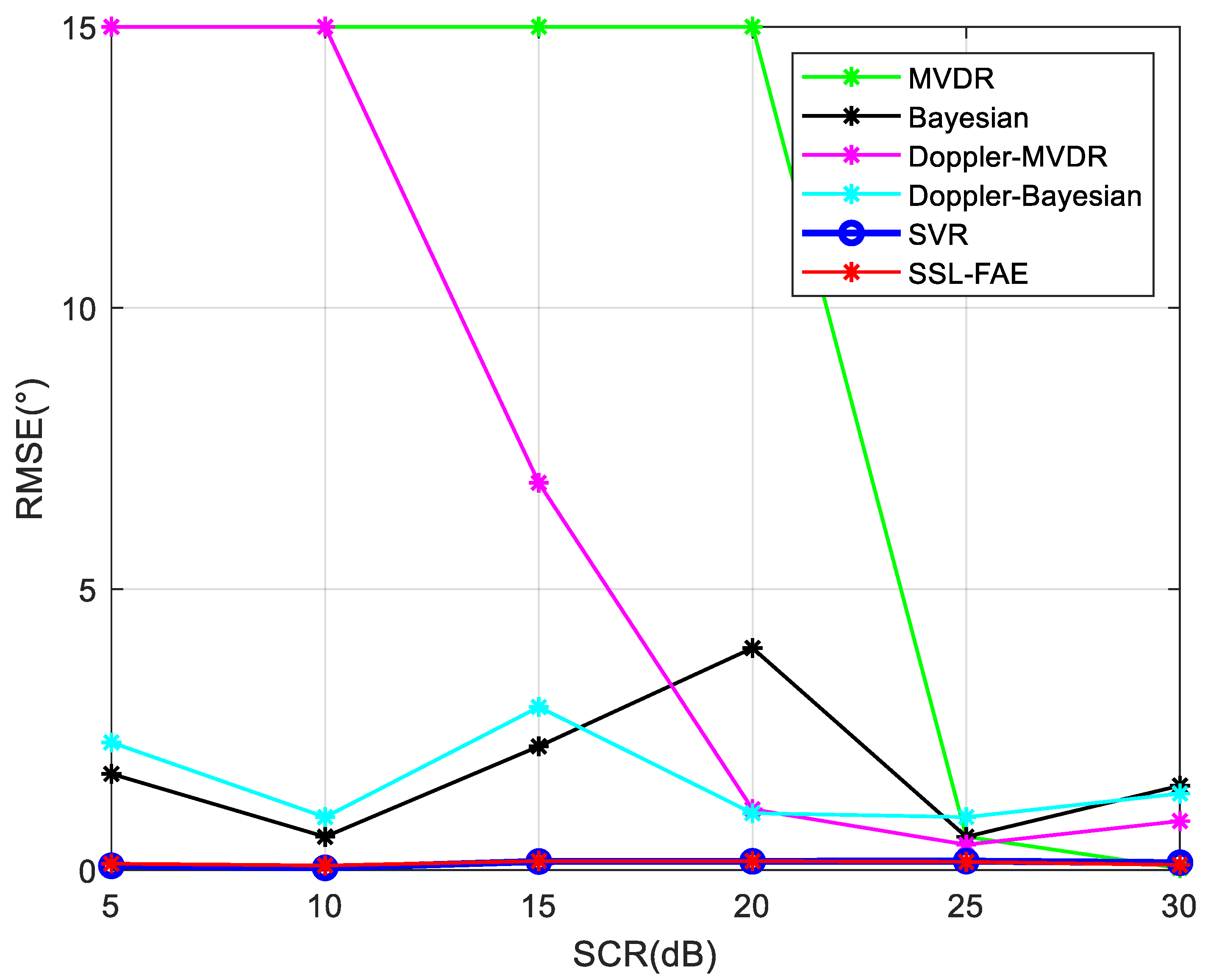
In this experiment, the performance of different algorithms under varying signal-to-clutter ratios (SCRs) is discussed. Different power levels of background clutter are introduced into the test dataset. The target angle is set at the center of scene, with the clutter backgrounds randomly distributed between −10° and 10°. Additionally, two pulse cancellation operations are conducted before estimation. A total of 500 Monte Carlo experiments are performed and the RMSE is utilized to evaluate the algorithms’ capability to mitigate clutter. The results are shown in Figure 12. The results indicate that, in terms of clutter adaptation capability, the MVDR method fails to accurately measure the target angle when the SCR is below 20 dB. Meanwhile, the Bayesian method, with L 1 -norm regularization, exhibits stronger clutter adaptation capability, but its angular accuracy in cluttered backgrounds struggles to achieve within 1 degree. In contrast, the proposed SSL-FAE method shows robust clutter resistance: at SCR above 0 dB, its angular measurement accuracy approaches 0.1 .
The above results indicate that the SSL-FAE and SVR demonstrate significant advantages in high-precision localization of moving targets. To further investigate, Table 3 illustrates their localization accuracy under different speed conditions. The SCR in the experiment is set to 10 dB.
At a relative speed of 40 m/s between the target and the platform, both SVR and the SSL-FAE experience significant performance declines. These declines are attributed to the limitations in the training set, where the target speed is randomly generated and does not fully encompass the test data. Consequently, some performance degradation on the test data is expected. However, for relative speeds ranging from 10 m/s to 160 m/s, the estimation accuracy of SVR and the SSL-FAE remains high.

3.4. Experiment 4

In this experiment, the efficiency of the algorithm using data from numerical simulations is tested. All algorithms are tested using the same dataset as in Experiment 1. For the training processes of SVR and the SSL-FAE, the selection of supervised and unsupervised data is consistent with the previous experiments. The test platform’s CPU model is a 12th Gen Intel(R) Core(TM) i9-12900H, and the testing software is Matlab R2022a. After completing 150 test runs, the average time spent for each method is calculated. The results are shown in Table 4.
The results indicate that, while the proposed algorithm achieves higher accuracy, its efficiency undergoes a decrease, primarily due to the longer training process. However, in practical applications, the efficiency of the angle estimation process is of primary importance. The proposed method maintains relatively high efficiency during the angle estimation process.

4. Conclusions

This paper proposes a semi-supervised learning framework for high-precision angle measurement with FLR. The proposed SSL-FAE method avoids complex intermediate modeling and establishes a direct mapping relationship between beam overlap scanning and the precise target azimuth angle, and a semi-supervised mechanism is introduced through manifold regularization, allowing for the mining of unlabeled data features in the manifold space. When the SNR reaches 20 dB, the target localization accuracy can be improved by more than double. Moreover, without the need to discretize the space, the SSL-FAE effectively solves the off-grid effect.

Author Contributions

Conceptualization, W.L., X.X. and Y.L.; methodology, W.L., Y.X. and Y.L.; software, Y.X. and X.X.; validation, Y.L. and W.L.; formal analysis, W.L. and H.T.; investigation, J.L. and J.Y.; resources, L.C., J.L. and J.Y.; data curation, F.Z., W.L. and H.T.; writing—original draft preparation, W.L. and Y.L.; writing—review and editing, H.T. and L.C.; funding acquisition, L.C. and F.Z. All authors have read and agreed to the published version of the manuscript.

Funding

This work is supported by the National Key R&D Program of China (2022YFB3901601) and National Natural Science Foundation of China (62201554).

Data Availability Statement

Data are contained within the article.

Acknowledgments

The authors would also like to express their gratitude to the anonymous reviewers and the editor for their constructive comments on this paper.

Conflicts of Interest

Authors Jie Liu and Junming Yu are employed by the company The 27th Research Institute of China Electronics Technology Group Corporation. The remaining authors declare that the research was conducted in the absence of any commercial or financial relationships that could be construed as a potential conflict of interest.

Abbreviations

The following abbreviations are used in this manuscript:
FLRForward-looking radar
SVRSupport vector regression
SNRSignal-to-noise ratio
APDAntenna pattern deconvolution
SVMSupport vector machines
ASPArray signal processing
SSL-FAESemi-supervised learning framework for FLR angle estimation
MVDRMinimum variance distortionless response
CSCompressive sensing
RKHSReproducing kernel Hilbert space
RBFRadial basis function
SCRSignal-to-clutter ratio

References

  1. Chen, H.; Li, Y.; Gao, W.; Zhang, W.; Sun, H.; Guo, L.; Yu, J. Bayesian Forward-Looking Superresolution Imaging Using Doppler Deconvolution in Expanded Beam Space for High-Speed Platform. IEEE Trans. Geosci. Remote Sens. 2022, 60, 1–13. [Google Scholar] [CrossRef]
  2. Zhang, Y.; Zhang, Y.; Huang, Y.; Li, W.; Yang, J. Angular Superresolution for Scanning Radar with Improved Regularized Iterative Adaptive Approach. IEEE Trans. Geosci. Remote Sens. 2016, 13, 846–850. [Google Scholar] [CrossRef]
  3. Chen, H.M.; Li, M.; Wang, Z.; Lu, Y.; Zhang, P.; Wu, Y. Sparse Super-resolution Imaging for Airborne Single Channel Forward-looking Radar in Expanded Beam Space via l p Regularisation. Electron. Lett. 2015, 51, 863–865. [Google Scholar] [CrossRef]
  4. Dropkin, H.; Ly, C. Superresolution for scanning antenna. In Proceedings of the 1997 IEEE National Radar Conference, Syracuse, New York, NY, USA, 13–15 May 1997; pp. 306–308. [Google Scholar]
  5. Li, Y.; Liu, J.; Jiang, X.; Huang, X. Angular Superresol for Signal Model in Coherent Scanning Radars. IEEE Trans. Aerosp. Electron. Syst. 2019, 55, 3103–3116. [Google Scholar] [CrossRef]
  6. Zhang, Y.; Zhang, Y.; Li, W.; Huang, Y.; Yang, J. Super-Resolution Surface Mapping for Scanning Radar: Inverse Filtering Based on the Fast Iterative Adaptive Approach. IEEE Trans. Geosci. Remote Sens. 2018, 56, 127–144. [Google Scholar] [CrossRef]
  7. Zhang, Y.; Jakobsson, A.; Zhang, Y.; Huang, Y.; Yang, J. Wideband Sparse Reconstruction for Scanning Radar. IEEE Trans. Geosci. Remote Sens. 2018, 56, 6055–6068. [Google Scholar] [CrossRef]
  8. Zhu, R.; Wen, J.; Xiong, X. Forward-looking imaging algorithm for airborne radar based on beam-space multiple signal classification. In Proceedings of the 2020 IEEE 20th International Conference on Communication Technology (ICCT), Nanning, China, 28–31 October 2020; pp. 1276–1280. [Google Scholar]
  9. Zha, Y.; Huang, Y.; Sun, Z.; Wang, Y.; Yang, J. Bayesian Deconvolution for Angular Super-Resolution in Forward-Looking Scanning Radar. Sensors 2015, 15, 6924–6946. [Google Scholar] [CrossRef] [PubMed]
  10. Zhang, Y.; Zhang, Q.; Li, C.; Zhang, Y.; Huang, Y.; Yang, J. Sea-Surface Target Angular Superresolution in Forward-Looking Radar Imaging Based on Maximum A Posteriori Algorithm. IEEE J. Sel. Top. Appl. Earth Obs. Remote Sens. 2019, 12, 2822–2834. [Google Scholar] [CrossRef]
  11. Zhang, Q.; Zhang, Y.; Huang, Y.; Zhang, Y. Azimuth Superresolution of Forward-Looking Radar Imaging Which Relies on Linearized Bregman. IEEE J. Sel. Top. Appl. Earth Obs. Remote Sens. 2019, 12, 2032–2043. [Google Scholar] [CrossRef]
  12. Yang, J.; Kang, Y.; Zhang, Y.; Huang, Y.; Zhang, Y. A Bayesian angular superresolution method with lognormal constraint for sea-surface target. IEEE Access 2020, 8, 13419–13428. [Google Scholar] [CrossRef]
  13. Duarte, M.F.; Baraniuk, R.G. Spectral compressive sensing. Appl. Comput. Harmon. Anal. 2013, 35, 111–129. [Google Scholar] [CrossRef]
  14. Chi, Y.; Scharf, L.L.; Pezeshki, A.; Calderbank, A.R. Sensitivity to basis mismatch in compressed sensing. IEEE Trans. Signal Process. 2011, 59, 2182–2195. [Google Scholar] [CrossRef]
  15. Herman, M.A.; Strohmer, T. General deviants: An analysis of perturbations in compressed sensing. IEEE J. Sel. Top. Signal Process. 2010, 4, 342–349. [Google Scholar] [CrossRef]
  16. Wang, M.; Yang, S.; Wu, S.; Luo, F. A RBFNN Approach for DoA Estimation of Ultra Wideband Antenna Array. Neurocomputing 2008, 71, 631–640. [Google Scholar] [CrossRef]
  17. Xiao, X.; Zhao, S.; Zhong, X.; Jones, D.L.; Chng, E.S.; Li, H. A Learning-Based Approach to Direction of Arrival Estimation in Noisy and Reverberant Environments. In Proceedings of the 2015 IEEE International Conference on Acoustics, Speech and Signal Processing (ICASSP), South Brisbane, QLD, Australia, 19–24 April 2015; pp. 2814–2818. [Google Scholar] [CrossRef]
  18. Chakrabarty, S.; Habets, E.A.P. Broadband Doa Estimation Using Convolutional Neural Networks Trained with Noise Signals. In Proceedings of the 2017 IEEE Workshop on Applications of Signal Processing to Audio and Acoustics (WASPAA), New Paltz, NY, USA, 15–18 October 2017; pp. 136–140. [Google Scholar] [CrossRef]
  19. Sun, Y.; Chen, J.; Yuen, C.; Rahardja, S. Indoor Sound Source Localization with Probabilistic Neural Network. IEEE Trans. Ind. Electron. 2018, 65, 6403–6413. [Google Scholar] [CrossRef]
  20. Liu, Z.M.; Zhang, C.; Yu, P.S. Direction-of-Arrival Estimation Based on Deep Neural Networks with Robustness to Array Imperfections. IEEE Trans. Antennas Propag. 2018, 66, 7315–7327. [Google Scholar] [CrossRef]
  21. Lo, T.; Leung, H.; Litva, J. Radial Basis Function Neural Network for Direction-of-Arrivals Estimation. IEEE Signal Process. Lett. 1994, 1, 45–47. [Google Scholar] [CrossRef]
  22. El Zooghby, A.; Christodoulou, C.; Georgiopoulos, M. A Neural Network-Based Smart Antenna for Multiple Source Tracking. IEEE Trans. Antennas Propag. 2000, 48, 768–776. [Google Scholar] [CrossRef]
  23. Randazzo, A.; Abou-Khousa, M.A.; Pastorino, M.; Zoughi, R. Direction of Arrival Estimation Based on Support Vector Regression: Experimental Validation and Comparison with MUSIC. IEEE Antennas Wirel. Propag. Lett. 2007, 6, 379–382. [Google Scholar] [CrossRef]
  24. Dehghanpour, M.; Vakili, V.T.; Farrokhi, A. DOA Estimation Using Multiple Kernel Learning SVM Considering Mutual Coupling. In Proceedings of the 2012 Fourth International Conference on Intelligent Networking and Collaborative Systems, Bucharest, Romania, 19–21 September 2012; pp. 55–61. [Google Scholar] [CrossRef]
  25. Ashok, C.; Venkateswaran, N. Support Vector Regression Based DOA Estimation in Heavy Tailed Noise Environment. In Proceedings of the 2016 International Conference on Wireless Communications, Signal Processing and Networking (WiSPNET), Chennai, India, 23–25 March 2016; pp. 99–102. [Google Scholar] [CrossRef]
  26. Venkateswaran, N.; Ashok, C. DOA Estimation of Near-Field Sources Using Support Vector Regression. In Proceedings of the 2016 IEEE Region 10 Conference (TENCON), Singapore, 22–25 November 2016; pp. 1570–1574. [Google Scholar] [CrossRef]
  27. Kabaoglu, N. Target Tracking Using Particle Filters with Support Vector Regression. IEEE Trans. Veh. Technol. 2009, 58, 2569–2573. [Google Scholar] [CrossRef]
  28. Ozer, S.; Cirpan, H.; Kabaoglu, N. Support Vector Machines Based Target Tracking Techniques. In Proceedings of the 2006 IEEE 14th Signal Processing and Communications Applications, Antalya, Turkey, 17–19 April 2006; pp. 1–4. [Google Scholar] [CrossRef]
  29. Kabaoğlu, N.; Çırpan, H.A. Wideband Target Tracking by Using SVR-based Sequential Monte Carlo Method. Signal Process. 2008, 88, 2804–2816. [Google Scholar] [CrossRef]
  30. Wu, L.L.; Huang, Z.T. Coherent SVR Learning for Wideband Direction-of-Arrival Estimation. IEEE Signal Process. Lett. 2019, 26, 642–646. [Google Scholar] [CrossRef]
  31. Wu, L. Array Signal Processing Based on Machine Learning. Ph.D. Thesis, National University of Defense Technology, Changsha, China, 2022. [Google Scholar]
  32. Perry, R.P.; DiPietro, R.C.; Fante, R.L. Coherent Integration with Range Migration Using Keystone Formatting. In Proceedings of the 2007 IEEE Radar Conference, Waltham, MA, USA, 17–20 April 2007; pp. 863–868. [Google Scholar] [CrossRef]
  33. Li, W.; Li, M.; Zuo, L.; Chen, H.; Wu, Y. Real aperture radar forward-looking imaging based on variational Bayesian in presence of outliers. IEEE Trans. Geosci. Remote Sens. 2022, 60, 1–13. [Google Scholar] [CrossRef]
  34. Chen, H.; Wang, Z.; Zhang, Y.; Jin, X.; Gao, W.; Yu, J. Data-driven airborne bayesian forward-looking superresolution imaging based on generalized Gaussian distribution. Front. Signal Process. 2023, 3, 1093203. [Google Scholar] [CrossRef]
  35. Benesty, J.; Chen, J.; Huang, Y. A generalized MVDR spectrum. IEEE Signal Process. Lett. 2005, 12, 827–830. [Google Scholar] [CrossRef]
  36. Wen, X.; Kuang, G.; Hu, J.; Zhan, R.; Zhang, J. Forward-looking imaging of scanning phased array radar based on the compressed sensing. Prog. Electromagn. Res. 2013, 143, 575–604. [Google Scholar] [CrossRef]
  37. Chen, L.; Tsang, I.W.; Xu, D. Laplacian Embedded Regression for Scalable Manifold Regularization. IEEE Trans. Neural Netw. Learn. Syst. 2012, 23, 902–915. [Google Scholar] [CrossRef] [PubMed]
  38. Hernández, N.; Biscay, R.J.; Talavera, I. Support Vector Regression Methods for Functional Data. In Progress in Pattern Recognition, Image Analysis and Applications; Rueda, L., Mery, D., Kittler, J., Eds.; Springer: Berlin/Heidelberg, Germany, 2008; Volume 4756, pp. 564–573. [Google Scholar] [CrossRef]
  39. Shen, X.J.; Dong, Y.; Gou, J.P.; Zhan, Y.Z.; Fan, J. Least Squares Kernel Ensemble Regression in Reproducing Kernel Hilbert Space. Neurocomputing 2018, 311, 235–244. [Google Scholar] [CrossRef]
  40. Beale, R.; Jackson, T. Neural Computing—An Introduction; CRC Press: Boca Raton, FL, USA, 1990. [Google Scholar]
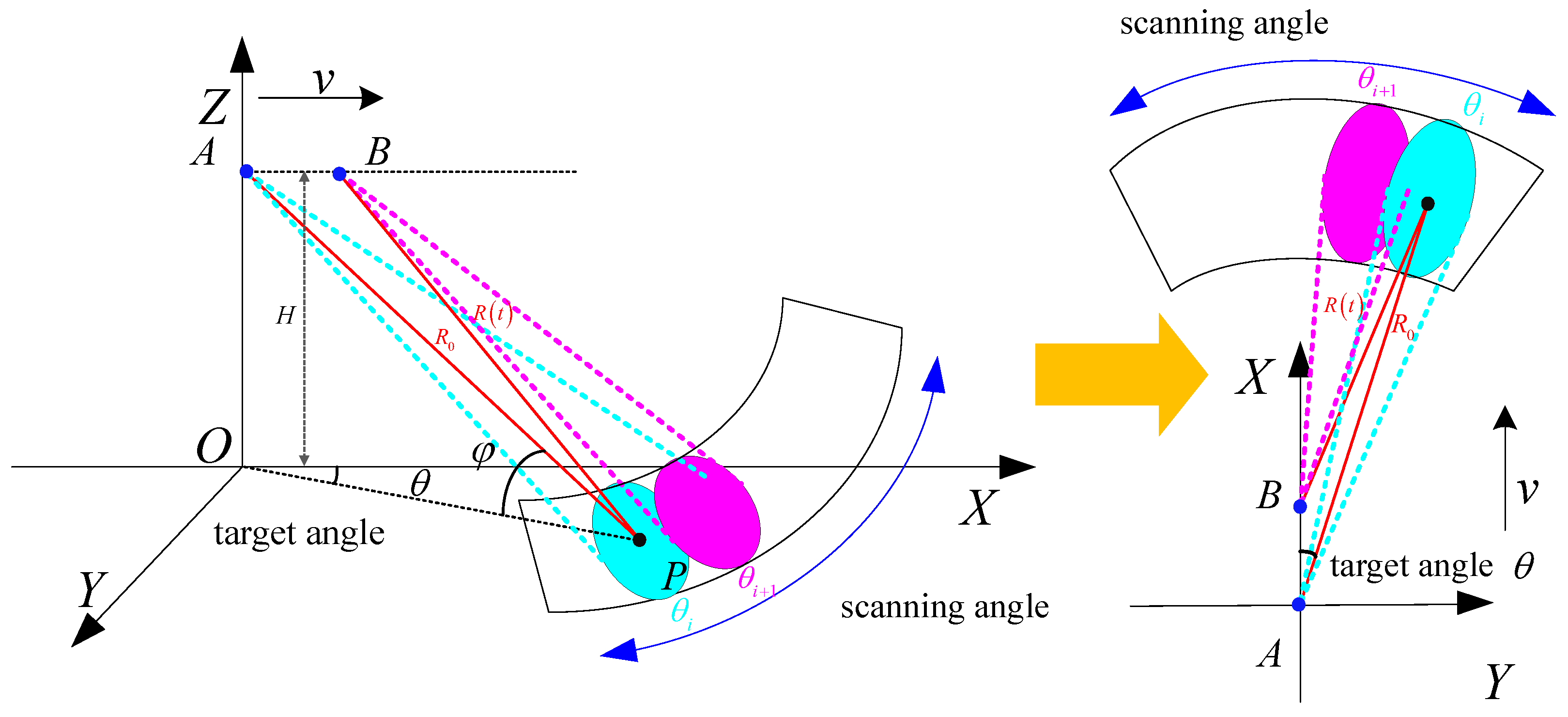
Figure 1. Geometry of forward-looking radar (FLR) for high-speed platform.
Remotesensing 16 02840 g001
Figure 2. Illustration of antenna pattern deconvolution in beamspace with FLR.
Remotesensing 16 02840 g002
Figure 3. Schematic diagram of semi-supervised learning framework for FLR angle estimation (SSL-FAE).
Remotesensing 16 02840 g003
Figure 4. The FLR angle estimation result with (a) MVDR, (b) Bayesian, (c) SVR, (d) Doppler-MVDR, (e) Doppler-Bayesian and (f) SSL-FAE (Case 1).
Remotesensing 16 02840 g004
Figure 5. The FLR angle estimation result (Case 2).
Remotesensing 16 02840 g005
Figure 6. The FLR angle estimation result (Case 3).
Remotesensing 16 02840 g006
Figure 7. The FLR angle estimation result (Case 4).
Remotesensing 16 02840 g007
Figure 8. The FLR angle estimation result (Case 5).
Remotesensing 16 02840 g008
Figure 9. The comparison of kernel functions of (a) Case 2, (b) Case 3 and (c) Case 4 with Case 1, and the comparison of combination coefficients of (d) Case 2, (e) Case 3 and (f) Case 4 with Case 1 when the target is at 10 .
Remotesensing 16 02840 g009
Figure 10. The comparison of kernel functions of (a) Case 2, (b) Case 3 and (c) Case 4 with Case 1, and the comparison of combination coefficients of (d) Case 2, (e) Case 3 and (f) Case 4 with Case 1 when the target is at 5.3 .
Remotesensing 16 02840 g010
Figure 11. Statistical performance of different algorithms.
Remotesensing 16 02840 g011
Figure 12. Performance of different algorithms under clutter conditions.
Remotesensing 16 02840 g012
Table 1. Simulation parameters.
ParameterSymbolValue
frequency f c 77 GHz
bandwidth B w 2 GHz
pulsewidthT2 μ s
pulse repetition frequencyPRF10 kHz
altitudeH100 m
velocityv0–250 km/h
Table 2. Parameters of SSL-FAE.
SymbolValue
λ H 1 × 10 5
λ M 1 × 10 3
η H 0.1
η M 0.1
Table 3. Localization accuracy for target at different speeds.
10 m/s40 m/s70 m/s100 m/s130 m/s160 m/s
SVR 0.00 × 10 7 0.27 × 10 7 0.00 × 10 7 0.00 × 10 7 0.00 × 10 7 0.00 × 10 7
SSL-FAE 0.00 × 10 7 0.24 × 10 7 0.00 × 10 7 0.00 × 10 7 0.00 × 10 7 0.00 × 10 7
Table 4. Efficiency of different algorithms.
MVDRBayesianDoppler–MVDRDoppler–BayesianSVRSSL-FAE
Training----0.3399 s1.5508 s
Estimation0.0874 s0.0055 s0.4118 s0.0073 s0.0016 s0.0028 s
Disclaimer/Publisher’s Note: The statements, opinions and data contained in all publications are solely those of the individual author(s) and contributor(s) and not of MDPI and/or the editor(s). MDPI and/or the editor(s) disclaim responsibility for any injury to people or property resulting from any ideas, methods, instructions or products referred to in the content.