Article

Vegetation Water Content Retrieval from Spaceborne GNSS-R and Multi-Source Remote Sensing Data Using Ensemble Machine Learning Methods

by
Yongfeng Zhang
1,
Jinwei Bu
1,*,
Xiaoqing Zuo
1,
Kegen Yu
2,
Qiulan Wang
1 and
Weimin Huang
3
1
Faculty of Land Resources Engineering, Kunming University of Science and Technology, Kunming 650093, China
2
School of Environment Science and Spatial Informatics, China University of Mining and Technology, Xuzhou 221116, China
3
Department of Electrical and Computer Engineering, Memorial University of Newfoundland, St. John’s, NL A1B 3X5, Canada
*
Author to whom correspondence should be addressed.
Remote Sens. 2024, 16(15), 2793; https://doi.org/10.3390/rs16152793
Submission received: 6 July 2024 / Revised: 24 July 2024 / Accepted: 29 July 2024 / Published: 30 July 2024

Abstract

:
Vegetation water content (VWC) is a crucial parameter for evaluating vegetation growth, climate change, natural disasters such as forest fires, and drought prediction. Spaceborne global navigation satellite system reflectometry (GNSS-R) has become a valuable tool for soil moisture (SM) and biomass remote sensing (RS) due to its higher spatial resolution compared with microwave measurements. Although previous studies have confirmed the enormous potential of spaceborne GNSS-R for vegetation monitoring, the utilization of this technology to fuse multiple RS parameters to retrieve VWC is not yet mature. For this purpose, this paper constructs a local high-spatiotemporal-resolution spaceborne GNSS-R VWC retrieval model that integrates key information, such as bistatic radar cross section (BRCS), effective scattering area, CYGNSS variables, and surface auxiliary parameters based on five ensemble machine learning (ML) algorithms (i.e., bagging tree (BT), gradient boosting decision tree (GBDT), extreme gradient boosting (XGBoost), random forest (RF), and light gradient boosting machine (LightGBM)). We extensively tested the performance of different models using SMAP ancillary data as validation data, and the results show that the root mean square errors (RMSEs) of the BT, XGBoost, RF, and LightGBM models in VWC retrieval are better than 0.50 kg/m2. Among them, the BT and RF models performed the best in localized VWC retrieval, with RMSE values of 0.50 kg/m2. Conversely, the XGBoost model exhibits the worst performance, with an RMSE of 0.85 kg/m2. In terms of RMSE, the RF model demonstrates improvements of 70.00%, 52.00%, and 32.00% over the XGBoost, LightGBM, and GBDT models, respectively.

1. Introduction

Vegetation water content (VWC) is the major factor influencing vegetation activity and biomass, and plays an important role in many key biogeochemical processes [1]. The vegetation water status represents the vegetation water at each unit scale, which can clearly show the wet and dry conditions of vegetation. Vegetation water status evaluation can accurately guide agricultural irrigation, predict yields, and drought assessment and forecast forest fires and other natural disasters [2]. Therefore, high precision and long time-series VWC product estimation, especially at critical phenological stages, is important for vegetation research. In addition, recent global climate change has a wide range of impacts on natural systems and climate change will complicate the relationship between the environment and vegetation, specifically, precipitation changes will affect the water cycle and water effectiveness of ecosystems [3]. Therefore, assessing the current status and trends of vegetation water and understanding its relationship with the environment are of great significance. The traditional method of VWC monitoring involves field measurements, which can only obtain a limited range of data, lack historical data, and are characterized by being destructive, time-consuming, and labor-intensive [4]. As an alternative, remote sensing (RS) technology can overcome above drawbacks of in situ monitoring, making it easier to obtain long time-series VWC spatial information.
Currently, most of the research focuses on estimating VWC information using RS data. Commonly used RS techniques include optical RS and microwave RS. Microwave RS can be categorized into active RS and passive RS. For optical RS, some empirical methods utilize biophysical parameters (e.g., surface temperature (SST) [5], solar-induced chlorophyll fluorescence (SIF) [6], normalized differential vegetation index (NDVI), leaf area index (LAI), enhanced vegetation index (EVI) [7], and vegetation optical depth (VOD) [8]), as well as significant correlations among other variables, to assess VWC. In addition, a decrease in VWC can lead to changes in spectral reflectance. The red, near-infrared (NIR), and short-wave infrared (SWIR) bands are sensitive to VWC stress and are used to compose various water indices (e.g., normalized difference water index (NDWI), simple ratio water index (SRWI), and plant water index (PWI)) for VWC retrieval [9]. Also, microwave RS data can also be used to estimate VWC, since the dielectric constants of water and dry vegetation differ significantly, and thus the distribution of water within vegetation impacts the interaction between microwave signals and vegetation. Previous studies on VWC retrieval based on microwave RS have predominantly concentrated on the identification of optimal auxiliary variables and their combinations. In active microwave RS, the role of backscattering coefficients and their computational metrics for diverse polarizations and combinations of incidence angles in constructing VWC models has been demonstrated [10,11]. In the realm of passive microwave RS, the optimal input parameters have been explored by comparing the retrieval accuracies of brightness temperature for various frequencies and polarizations [12].
Nevertheless, although optical RS retrieval yields higher spatial resolution of VWC, optical images are susceptible to cloudiness, resulting in missing information. In contrast, microwave signals, with their longer wavelengths and superior penetration capabilities, remain unaffected by cloud cover. However, there are certain limitations to consider. Apart from the coarse spatial resolution of microwave data, vegetation information derived from microwave signals is influenced by factors such as ground roughness and soil moisture (SM) [13]. Although there have been studies in recent years to combine the two to explore higher-resolution VWC estimation [14], the notable discrepancy in spatial resolution between optical and microwave RS products often results in limited accuracy and spatial resolution in the fusion results for practical applications. Consequently, alternative and improved methods are required for VWC retrieval.
The Global Navigation Satellite System Reflectometry (GNSS-R) technique, a passive bistatic radar RS technique, relies on the reception of signals of opportunity reflected from the Earth’s surface to infer the properties of the reflecting surface itself [15]. CYGNSS science data products include L1, L2 and L3 products: L1 products comprise bistatic radar cross sections (BRCS) of the Earth’s surface; L2 products include ocean surface wind speed and mean square slope; ocean surface heat flux and ocean surface wind speed (NOAA); and L3 products include gridded ocean surface wind speed and mean square slope, ocean microplastic concentration, storm-centric grids, 6-hourly and daily SM UC (university of california) berkeley watermask, and merged (MRG) storm grids. In addition, the latter also include full delay-Doppler maps (DDMs) and raw intermediate frequency [16]. With the advancement of GNSS-R technology, L1-level scientific data products have been widely utilized in various respects, such as for SM [17,18], wind speed [19], swell [20], sea ice [21,22], ocean tides [23], snow depth [24], surface water fraction (SWF) [25], and vegetation [26] retrieval. For vegetation monitoring, many researchers have utilized GPS reflection signals to retrieve VWC, as the amplitude of direct and reflected GNSS interference signals is related to variation in VWC. Therefore, GNSS-R is an alternative technology to obtain long time-series VWC information [26]. In the last few years, several experiments have been proposed and realized utilizing ground-based, airborne, and spaceborne platforms. Regarding ground-based platforms, the most representative studies are the GPS signal-to-noise ratio (GPS-SNR) method and the interference pattern technique (IPT). The GPS-SNR method involves utilizing multipath information received by Plate Boundary Observatory (PBO) stations to acquire SNR data, extract essential reflector height, phase, and amplitude information, and then perform retrieval of relevant vegetation indices (e.g., VWC and normalized microwave reflectance index (NMRI)) [27,28], whereas IPT technology utilizes an enhanced GPS receiver that builds upon existing geodetic GNSS receivers. With this approach, Rodriguez-Alvarez et al. [29,30] specifically focused on improvement in antenna polarization and employed vertically polarized antennas to obtain surface characteristics. To improve the retrieval accuracy, Loria et al. [27] extended the approach by using horizontally polarized antennas and interference waveforms to obtain vegetation height information through notch location and numerical antenna information. In terms of airborne GNSS-R, Pierdicca et al. [31] and Egido et al. [32] demonstrated the sensitivity of GNSS-R signals to SM and vegetation biomass through the development of a terrestrial GNSS-R data simulator. They found that for low-altitude GNSS-R airborne platforms, the reflectance polarization ratio exhibited high stability relative to surface roughness, providing reliable observability for SM. Additionally, they observed that the homopolar reflectance coefficient showed stable sensitivity to forest aboveground biomass (AGB). On this basis, Motte et al. [33] and Zribi et al. [34] demonstrated through the global navigation satellite system reflectometer instrument (GLORI) that the correlation between forest parameters in left-hand circular polarization (LHCP) and GNSS reflectivity ( Γ L R ) or polarization ratio (PR) at high elevation angles (70–90°) yields high sensitivity. Among these, PR showed the greatest potential for reflectivity compared to LHCP. To further enhance the analysis, Jia and Savi et al. [35] added right-hand circular polarization (RHCP) to this to study vegetation and SM fluctuations using three polarization observables, which showed good correlations with terrain type. In terms of simulation, Park et al. [36] developed a comprehensive end-to-end simulator that generates synthetic DDMs reflected over land. In recent studies, Munoz-Martin et al. [37] utilized an airborne microwave interferometric reflectometer (MIR) GNSS-R instrument to perform vegetation canopy height retrieval at L1 and L5 using a neural network algorithm, which showed similar performance at L1 and L5.
Recently, the utilization of spaceborne GNSS-R technology for monitoring vegetation parameters has attracted significant attention in the scientific community [38,39]. Compared to traditional monostatic radars, this method offers a significant advantage in estimating vegetation parameters because the signal response of biomass does not saturate as easily as in monostatic radars [40]. Therefore, monitoring vegetation parameters using this RS method has advantages that cannot be compared with traditional RS methods. Currently, the work on spaceborne GNSS-R vegetation monitoring primarily focuses on the study of AGB using the CYGNSS mission. For example, Camps et al. [41] used TDS-1 data to qualitatively analyze the effects of SM, roughness, terrain, and volume scattering on GNSS-R data. They also analyzed the impacts of different surface SM around the Earth and the large-scale NDVI sensitivity to GNSS-R scattered energy. Carreno-Luengo et al. [42] employed SMAP reflectometry (SMAP-R) to investigate biomass and SM, demonstrating the SNR, PR, leading edge slope (LES), and trailing edge slope (TES) sensitivity to the effects of Earth terrain and AGB. Similar studies were conducted by Santi et al. [43,44] on global SM and AGB retrieval using CYGNSS data and artificial neural networks (ANN). Carreno-Luengo et al. [45] used CYGNSS L1 data to simulate and analyze the relationship between GNSS-R variables and AGB. Additionally, Santi et al. [46] employed TDS-1 and CYGNSS data in conjunction with ANN methods to investigate AGB and assessed its sensitivity to forest parameters by directly comparing it with VOD. The study utilized incident angle, SNR, longitude, and latitude information from the global map as input variables for the ANN, with local and global retrieval. The results revealed that this method demonstrates high accuracy in estimating biomass and tree height. In addition, Pilikos et al. [47] proposed a deep learning (DL) retrieval model incorporating full DDM surface reflectance for fast and continuous biomass retrieval. Although research on VWC has focused on using spaceborne GNSS-R variables to establish sensitivity analysis with VWC, current work is in the early research stage of qualitative analysis, and more regrettably, it lacks the discovery of the physical mechanisms behind it, in addition to very little research having been carried out on quantitative retrieval of VWC. Recently, Chen et al. [48] used the slope and intercept derived from the tau-omega model combined with geographic location and land cover information to retrieve VWC by establishing linear models and ANN models. Although ANN models have certain potential in handling complex features and pattern recognition, they are mostly considered black box models, making it difficult to debug, interpret, and diagnose model problems.
To summarize, in terms of retrieval of spaceborne GNSS-R vegetation parameters (especially VWC retrieval), previous studies utilized a single value for equivalent surface reflectivity, computed from the maximum power received at the platform for each location, so we use the latitude and longitude collected by CYGNSS as an input to enable the model to learn the regional VWC patterns and behaviors. However, location alone is not sufficient because the retrieval model predictions are very coarse and completely ignore small-scale variability. Since CYGNSS observations are correlated with VWC, several other auxiliary parameters (e.g., SNR, normalized bistatic radar scattering cross section (NBRCS), LES, range correction gain (RCG), etc.) are also utilized to enhance the VWC retrieval model performance. However, using only the peak power does not utilize the additional information in the DDM structure, and the peak power of the GNSS-R signal will not be available if the observation area contains a water body. This is because the power reflected from the water surface determines the amplitude of the reflected signal [49]. Inspired by this and considering the differences in the structure of the DDM for different VWC values, we employ the entire DDM for VWC estimation, supplemented by additional input data such as latitude, longitude, SNR, and SM. Theoretically, the relationship between GNSS-R observations and surface geophysical parameters is complex, and integrated machine learning (ML) can effectively simulate the complex relationship between GNSS-R observations and surface geophysical parameters [50]. This study builds a VWC retrieval model based on integrated ML tree models, i.e., bagging tree (BT), gradient boosting decision tree (GBDT), extreme gradient boosting (XGBoost), random forest (RF), and lightweight gradient boosting machine (LightGBM). Although some studies have successfully used integrated ML methods for terrestrial GNSS-R applications (e.g., SM retrieval [51,52]), they have not been used for VWC quantitative retrieval model construction.
This article integrates key information, such as the BRCS, effective scattering area, CYGNSS variables, and surface auxiliary parameters. Based on five integrated ML algorithms (BT, GBDT, XGBoost, RF, and LightGBM), a local high-resolution spaceborne GNSS-R VWC retrieval model is constructed for the first time. Compared with previous research, this paper mainly has the following innovative points.
(1)
On the basis of considering DDM, CYGNSS variables and surface auxiliary parameter information, the influence of images (BRCS, effective scattering area) was also considered.
(2)
We consider the importance of seasonal parameters in building a VWC retrieval model.
(3)
We explore the impact of different input strategies on the model, and it is proven that GNSS-R variables have a positive impact on improving the accuracy of VWC retrieval.
(4)
In addition to selecting Australia as the research area, we also selected southeastern South America and southeastern Africa to verify the applicability and universality of its model.
(5)
This article removes the influence of inland water bodies on VWC retrieval.
The rest of the paper is organized as follows. Section 2 describes the datasets used in the paper and the data processing methods. Section 3 describes the construction of the integrated ML model for VWC retrieval. Section 4 validates and analyzes the performance of the proposed VWC retrieval model and comprehensively discusses the VWC retrieval results from four angles (e.g., different input variable strategies, different seasons, spatial variations, and different vegetation covers). Section 5 summarizes the main conclusions of the paper.

2. Dataset Description and Data Processing

2.1. Dataset Description

This article utilizes a total of seven datasets from 1 January to 31 December 2021, CYGNSS data, SMAP data, MODIS land cover type data (MCD12C1), GPM precipitation data, ECMWF data, AMSRU data, and Global Surface Water (GSW) data, as shown in Table 1. We first perform quality control on these seven datasets, as detailed in Section 2.2 below. The seven datasets use linear interpolation methods on a time scale to maintain high consistency. Then, the bilinear interpolation method is used in space to interpolate it into the EASE Grid 2.0 9 km × 9 km grid.

2.1.1. CYGNSS L1B Datasets

This article utilizes the first level data of CYGNSS-L1-V3.0. The CYGNSS constellation contains eight microsatellites (CY01, CY02, CY03, CY04, CY05, CY06, CY07, and CY08) that offer GNSS-R data coverage across the pantropical region (from 38° S to 38° N). In this study, we used BRCS, eff_scatter, power_analog, ddm_snr, ddm_nbrcs, ddm_les, sp_rx_gain, gps_eirp, rx_to_sp_range, tx_to_sp_range, sp_lat, sp_lon, sp_inc_angle, and RCG variables from L1-level metadata for VWC retrieval.

2.1.2. Reference and Validation Data

The VWC used in this paper is provided by SMAP data, which is based on the land cover and NDVI derived from MODIS. The SMAP mission was launched on 31 January 2015 using L-band passive radiometers and active radars to measure global high-resolution SM and freeze–thaw conditions every 2–3 days. SMAP consists of four levels of products, with levels 1–4 of auxiliary data products used to create SMAP L1, L2, L3, and L4 products, respectively. This article uses the SMAP enhanced L3 radiometer Global Daily 9-km EASE Grid.

2.1.3. Auxiliary Data for the Retrieval Process

(1)
GPM IMERG precipitation product
Precipitation has been proven to be related to the water and growth status of vegetation [59], and is therefore used as a climate factor in this article. We selected GPM-IMERG precipitation data. GPM-IMERG was launched in 2014 as a follow-up project to the Tropical Precipitation Measurement Mission (TRMM). GPM-IMERG adopts a three-level multi-satellite precipitation algorithm that combines intermittent precipitation estimation from all constellation microwave sensors, infrared observation data from geostationary satellites, and monthly precipitation data from rain gauges. GPM-IMERG has three types of products, namely, IMERG Early Run (IMERG-E) (real-time product with a delay of about 4 h), IMERG Late Run (IMERG-L) (near real-time processing product with a delay of about 14 h), and IMERG Final Run (IMERG-F). The spatial resolution of these three products is 0.1° × 0.1°, and the temporal resolution includes 1 month, 1 day, and 30 min. In this study, the IMERG-L product with a daily time resolution is utilized to develop a VWC retrieval model.
(2)
ECMWF data
The Copernicus Climate Change Service (C3S) climate database provides users with reanalysis data for ECMWF. This article uses ERA5, which includes hourly land data from 1950 to the present, with a spatial resolution of 0.1° × 0.1°. ERA5 Land is a surface data product provided by the European Centre for Medium Range Weather Forecasts (ECMWF) and is a derivative of ERA5. The ERA5 Land data product includes a wide range of land surface variables (2 m dew temperature, 2 m temperature, LAI, SST, etc.), covering different time scales (hours, days, etc.) and spatial resolutions. This article extracts the SST from its metadata. Previous research conducted by Zhang et al. [60] demonstrated that SST significantly affects the correlation between CYGNSS reflectance and SM, and for vegetation monitoring, Calvet et al. [61] demonstrated the feasibility of brightness temperature for monitoring VWC, and showed that it affects canopy reflectance. Therefore, this article also considers the influence of SST variables on VWC retrieval.
(3)
AMSRU data
The AMSRU data used in this article are daily global land parameters derived from AMSR-E and AMSR2 version 3. This dataset includes satellite retrieval geophysical parameter files generated by the Advanced Microwave Scanning Radiometer Earth Observation System (AMSR-E) instrument on NASA’s Aqua satellite and the Advanced Microwave Scanning Radiometer 2 (AMSR2) sensor on the JAXA GCOM-W2 satellite. Geophysical parameters include a 60-day open water coverage fraction (fw) and daily (non-smooth) open water estimates (fwns). The minimum and maximum values of daily SST (Tmn and Tmx, ~2 m height), VOD in the x-band (10.7 GHz), surface (10.7 GHz) soil volumetric humidity (vsm), total atmospheric column precipitation, surface atmospheric vapor pressure difference (VPD, ~2 m altitude), and daily SM are considered. This generates a global EASE Grid (v1) projection with a resolution of 25 km and a time resolution of 1 day. In this study, we used daily parameters of SM, which provides water to vegetation and plays a vital role in vegetation photosynthesis, carbon fluxes, and leaf water potential [62].
(4)
Land cover data (MCD12C1)
This study utilized the International Geosphere Biosphere Programme (IGBP) land classification dataset. This product covers a valid timeframe of 2001–2022 with a spatial resolution of 0.05° × 0.05° and a temporal resolution of 1 year. As shown in Figure 1, we selected 17 IGBP categories representing different vegetation distributions in 2021 and used this dataset to facilitate the validation of the proposed modeling algorithm’s ability to perform VWC retrieval on different vegetation covers.
(5)
GSW data
The GSW dataset is a water dataset created by the European Commission’s Joint Research Center in the Copernicus project. The dataset is generated from land satellite images and maps the location and time distribution of water surfaces worldwide over the past 3.8 years, providing statistical data on the range of and changes in these water surfaces. Due to the presence of inland open water bodies on the surface, which can affect the scattering of GNSS signals, it is necessary to eliminate observations of areas with relatively high percentages of open water bodies [63]. This article mainly uses the seasonal data provided by the GSW dataset to remove the impact of inland open water bodies on VWC retrieval. One pixel of this product represents the length of time that open water exists in a year (0–12 months), and the water content percentage of each 3 km grid is calculated as the percentage of a 30 m grid within a 3 km frame in the presence of permanent or seasonal water. We use this water content percentage to filter CYGNSS data samples. Then, a 2% threshold is applied to remove the 3 km grid cells of inland water bodies [64].

2.2. Quality Control of Spaceborne GNSS-R Observation Data and Reflectivity Calculate

2.2.1. Quality Control of GNSS-R Data

In order to better perform the retrieval of VWC, we need to control the quality of CYGNSS observation data and remove data with poor quality and anomaly. In this study, we set the values that meet the conditions to 1 based on specific indicators in the report, and 0 otherwise [64]. In addition, we discarded the CYGNSS observation data with antenna gain < 0, BRCS uncertainty below 1, and RCG less than 0 from the input dataset [65] and those with an incident angle greater than 65° [66] to avoid DDM containing noise, as shown in Table 2. The quality control procedures for SMAP data products are detailed in Supplementary Materials.
The RCG can be used as an effective indicator of the quality of received scattering signals [67]. It is defined as:
RCG = G R 10 27 R T R R 2
where G R is the receiver antenna gain pattern. R T and R R are the distances between the nominal SP and the GNSS transmitter/receiver, respectively. The unit of RCG is 10 27 × d B i × M 4 .

2.2.2. CYGNSS Reflectivity Calculation

Reflectivity, a crucial characteristic parameter of land GNSS-R observation data, finds extensive application in SM and biomass retrieval studies. In this article, it is assumed that signals from land primarily result from coherent reflections on the surface, which are ultimately determined by reduced surface roughness and vegetation attenuation. The CYGNSS reflectivity is the pivotal observational parameter employed for estimating VWC, and it is defined as [68]:
Γ = P D D M N M 4 π 2 R R + R T 2 G R λ 2 P T G T
where P D D M represents the peak value of the DDM of the analogue scattered power. N M represents the DDM noise floor, which is estimated as the mean value of the DDM subset in the absence of signal. G T P T represents the effective isotropic radiated power (EIRP). λ is the carrier wavelength. The other parameters have been described earlier.
In addition to the variables mentioned above, some informative data are provided in Table 3 that can be used as auxiliary input to the SM retrieval algorithm or for the calculation of other observables [69].

3. Construction of Ensemble ML Model for Retrieval of VWC

In this subsection, we will explain the construction process of each of the five ML models (RF, XGBoost, GBDT, LightGBM, and BT) used in detail.
For a detailed definition of RF, please refer to [70]. In this paper, we set its parameter n_estimators (maximum number of iterations) to 50, min_samples_split (minimum number of samples in leaf nodes) to 2, and min_samples_leaf (minimum number of leaves in a tree) to 1.
XGBoost is a scalable end-to-end tree boosting system that has been widely used in classification, regression, and other ML tasks. The principle of constructing a VWC model using the XGBoost algorithm can be found in [71]. However, in this paper, the parameters n_estimators and important_type are configured as 50 and “gain,” respectively.
GBDT is an iterative decision tree algorithm proposed by Friedman in 2001 [72], which consists of multiple decision trees. The principle of constructing a VWC model based on its algorithm can be found in [73]. However, in this paper, the values of the four parameters of n-estimators, learning-rate (weight reduction coefficient ν for each weak learner), subsample (subsampling), and loss (loss function) are set to 50, 1, 0.6, and deviation, respectively.
LightGBM [71] is an efficient GBDT that helps improve the efficiency of models when the variable dimensions of data samples are high and the data size is large. Compared to XGBoost, LightGBM has faster computing speed and less memory consumption. It is worth noting that the values of n_estimators (number of boosted trees to fit), num_leaves (maximum tree leaves for base learners), and learning_rate (boosting learning rate) are set to 50, 31, and 0.1, respectively.
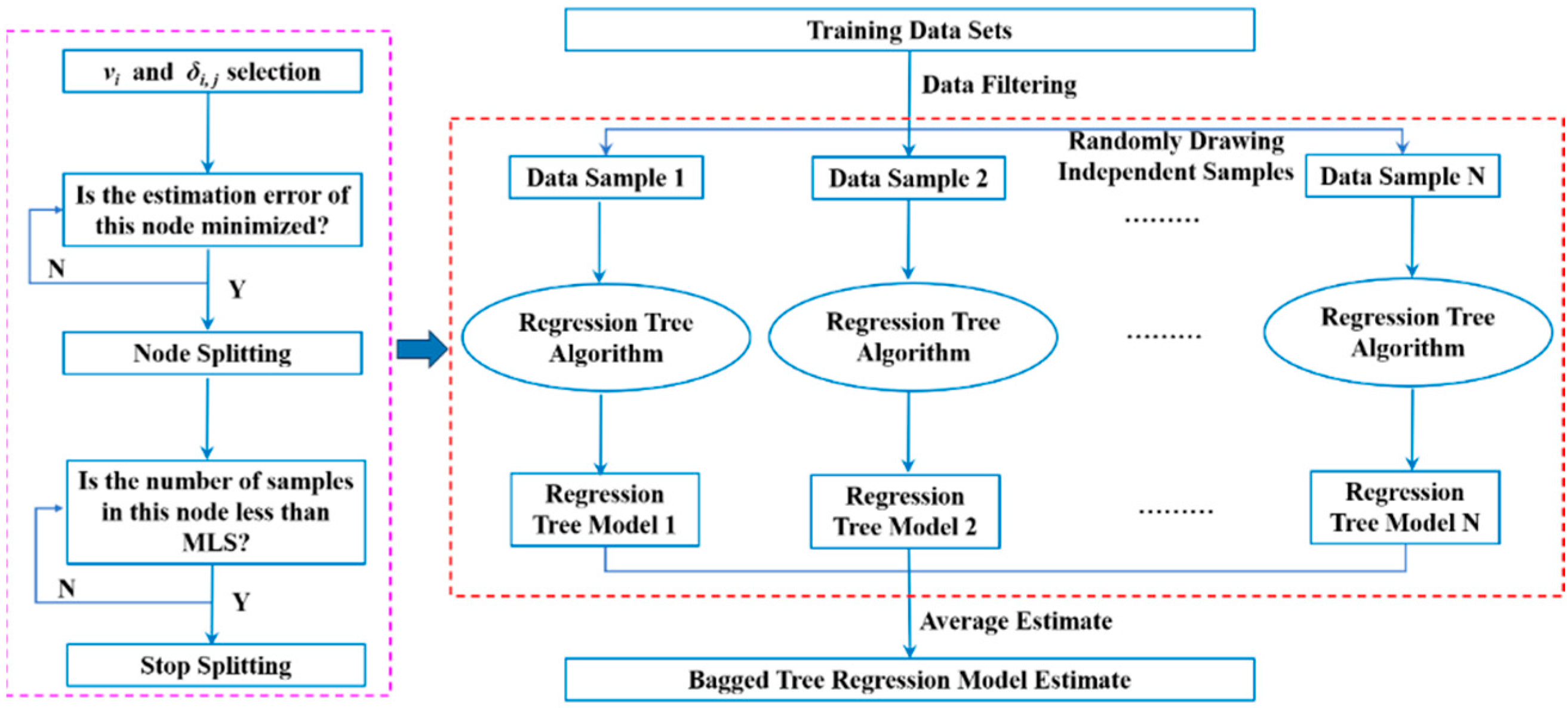
BT is one of the most popular ensemble algorithms based on the concepts of bootstrapping and aggregation. Figure 2 shows the BT algorithm process. In bagging, the training set is randomly sampled n times and replaced to generate n training sets of the same size as the original training set. It extracts the training set from the original data and uses bootstrapping to randomly select a certain number of training samples from the initial sample set of each cycle [74]. We generate a large number of comparable datasets through resampling and replacement and generate a regression tree without pruning and averaging, resulting in a decrease in the RMSE of the model [75]. In this article, n = 30 , and we use training set data samples to construct the model, where the m t h is defined as follows:
S m = v 1 m , v 2 m , , v 16 m ; V W C m ^
where S m is the m t h sample, v 1 m , v 2 m , , v 16 m is the value of the input variables, and V W C m ^ is the true value of VWC. According to the optimal segmentation variable ν i and optimal segmentation value δ i , j among the 16 input variables, all samples in the node are divided into two sub-nodes: Node 1 = S N 1 1 ,   S N 1 2 ,   S N 1 3 ,   , and Node 2 = S N 2 1 ,   S N 2 2 ,   S N 2 3 ,   , . All samples in the two child nodes will be assigned an VWC estimate ( V W C N 1 , V W C N 2 ), which can be calculated as:
V W C N 1 = 1 K 1 p = 1 K 1 V W C N 1 p ^
V W C N 2 = 1 K 2 q = 1 K 2 V W C N 2 q ^
where N 1 and N 2 are the training sets and K 1 and K 2 are the sample numbers of N 1 and N 2 , respectively. The selection criteria for ν i and δ i , j are to minimize the estimation error of the node as:
EE = min v i , δ i , j p = 1 K 1 V W C N 1 p ^ V W C N 1 2 + q = 1 K 2 V W C N 2 q ^ V W C N 2 2
where E E is the estimation error of the node, and then the two sub-nodes ( N o d e 1 and N o d e 2 ) continue to split. When the number of samples in the node is fewer than or equal to the minimum leaf size (MLS, which is set to 4), this node stops splitting.
It should be noted that in the model construction process above, we found that the n-estimators parameter in the four algorithms (GBDT, XGBoost, RF, and LightGBM) has a large impact on the performance of the model. A larger value of this parameter can improve the model’s ability to fit the training set; however, it may also exacerbate overfitting. Conversely, if the setting is too low, it may lead to model underfitting. In order to compare the performance of different models under the same training parameter settings and to ensure that each model achieves the best training performance, we tested the number of iterations of different models and found that the retrieval performance of the four models is best when the number of iterations is 50. For the other parameter settings of the four models, we retained the original design and characteristics of the algorithms.

4. Model Verification and Performance Analysis

4.1. Evaluation Indicators and Verification Strategies

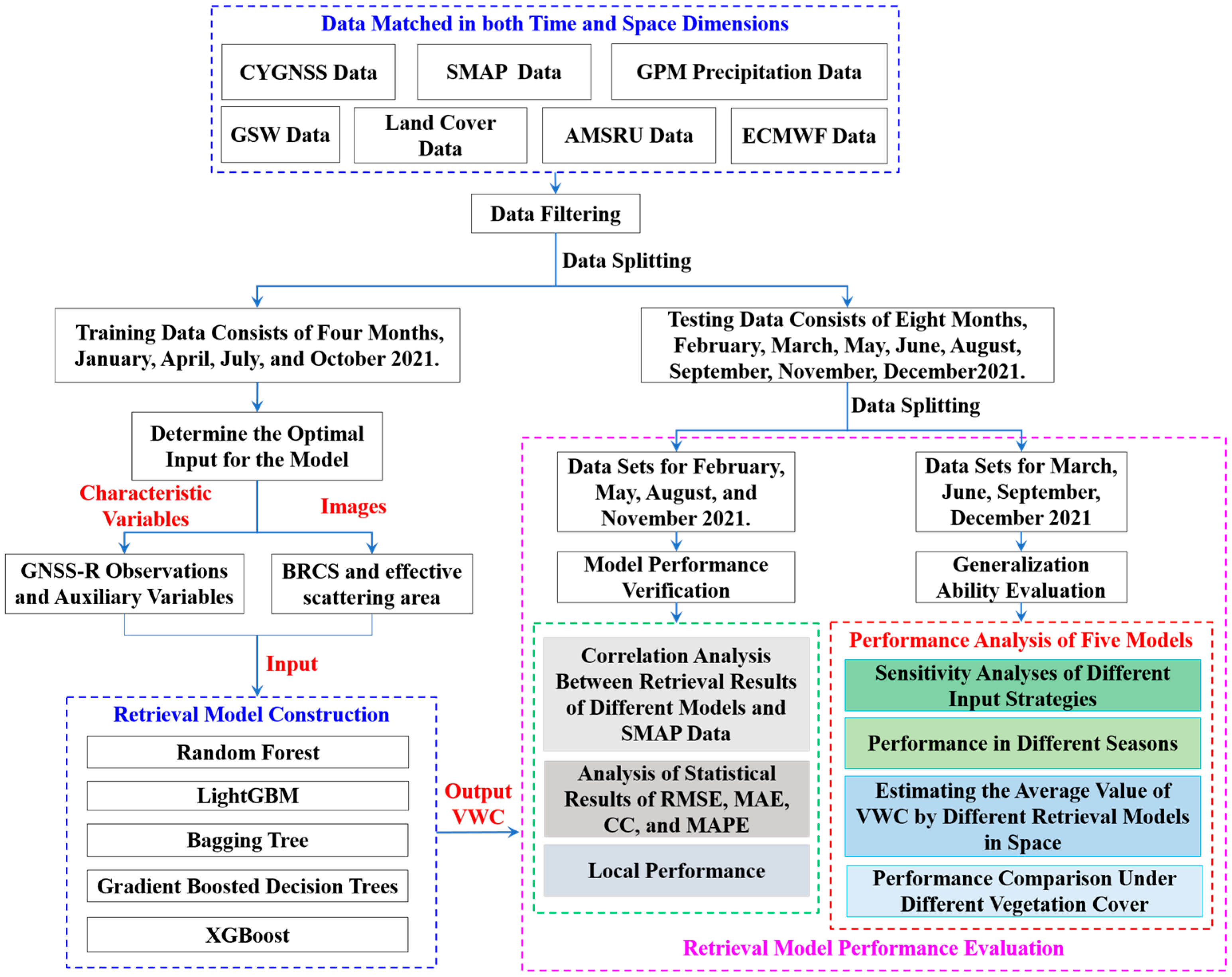
This section thoroughly analyzes VWC retrieval models to assess the applicability and universality of the five ML algorithms (e.g., BT, GBDT, XGBoost, RF, and LightGBM) introduced in this study. To verify the generalization capability of various retrieval methods on unseen data, we utilize SMAP auxiliary data from MODIS products for training and testing. In our study, we selected 4 months (accounting for about 33.3% of the total samples) of the data for training and 8 months (accounting for about 66.7% of the total samples) of the data for testing in consideration of model fitting performance and model retrieval performance. This ratio was determined as a trade-off between the need to have a training dataset sufficiently representative of the behavior of the overall data and the need to keep the computational time for the network determination acceptable. We divided the test dataset into two parts: the first part was used to cross-validate the retrieval performance of the five constructed models with the SMAP data, and the second part was used to discuss the performance of the retrieval model of VWC in terms of four aspects (i.e., correlations among different input variable strategies, different seasons, spatial variations, and different vegetation covers). To evaluate the VWC retrieval performance of the five models, we used the RMSE, Pearson correlation coefficient (R), mean absolute error (MAE), and mean absolute percentage error (MAPE) indicators. These indicators are defined in [76]. Table 3 presents the input GNSS-R variables of the VWC retrieval model developed in this thesis (for a detailed description of CYGNSS-related variables, please refer to [16]). Figure 3 depicts the flowchart of the evaluation method for the VWC retrieval model.

4.2. Comparison with SMAP Data

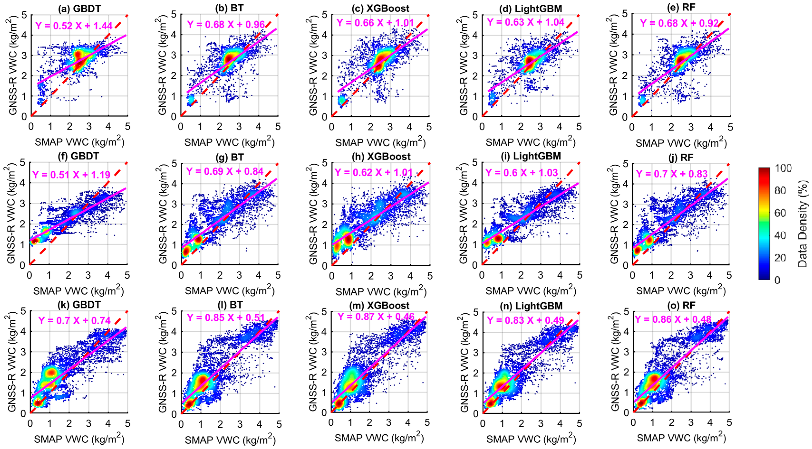
This article uses SMAP ancillary VWC data as reference data, and inputs DDM images, GNSS-R variables, and surface auxiliary parameters into five models (GBDT, BT, XGBoost, LightGBM, and RF models) for comparative verification. The performance testing of VWC retrieval in this article was conducted on a test dataset, where the test data, training data, and validation data were independent of one another. This is very suitable for improving the robustness and generalization ability of the model performance. Figure 4 illustrates the scatter density plots of VWC retrieved by the five models. Additionally, the linear fit equation ( Y = a X + b ) that describes the relationship between the model retrieved VWC and the SMAP VWC is provided. Table 4 depicts the statistical results of RMSE, MAE, R, and MAPE for different models.
Figure 4 shows that the correlation between the VWC retrieved by the BT model and RF model method and the SMAP VWC is relatively superior to that of the other three models. The BT model and RF model method exhibit the highest degree of concentration near the 1:1 reference line (e.g., y = x ). This suggests that the BT model and RF model achieve relatively good performance in retrieving local VWC, and the performance ranking of these models are BT > RF > GBDT > LightGBM > XGBoost. Additionally, compared with SMAP ancillary VWC data, XGBoost, LightGBM, and GBDT models have narrower dynamic ranges and weaker correlations for certain VWC values. The main reason is that in integrated ML, different models often have different hyperparameters, and the setting of these hyperparameters can affect the complexity, generalization ability, and performance of the model. Therefore, XGBoost, LightGBM, and GBDT models may have limited predictive ability for VWC values. The VWC retrieval performances of the BT model and RF model are consistently similar, with only a 1.75% difference in MAPE. It can be observed from Table 4 that the BT model and RF model exhibit better accuracy compared to the XGBoost, LightGBM, and GBDT models: in terms of RMSE, this is improved by 70.00%, 52.00%, and 32.00%, respectively; in terms of MAE, this is improved by 121.88%, 93.75%, and 46.88%, respectively, in terms of MAPE, this is improved by 200.95%, 176.99%, and 67.57%, respectively; and in terms of R value, this is improved by 14.29%, 6.59%, and 7.69%, respectively.
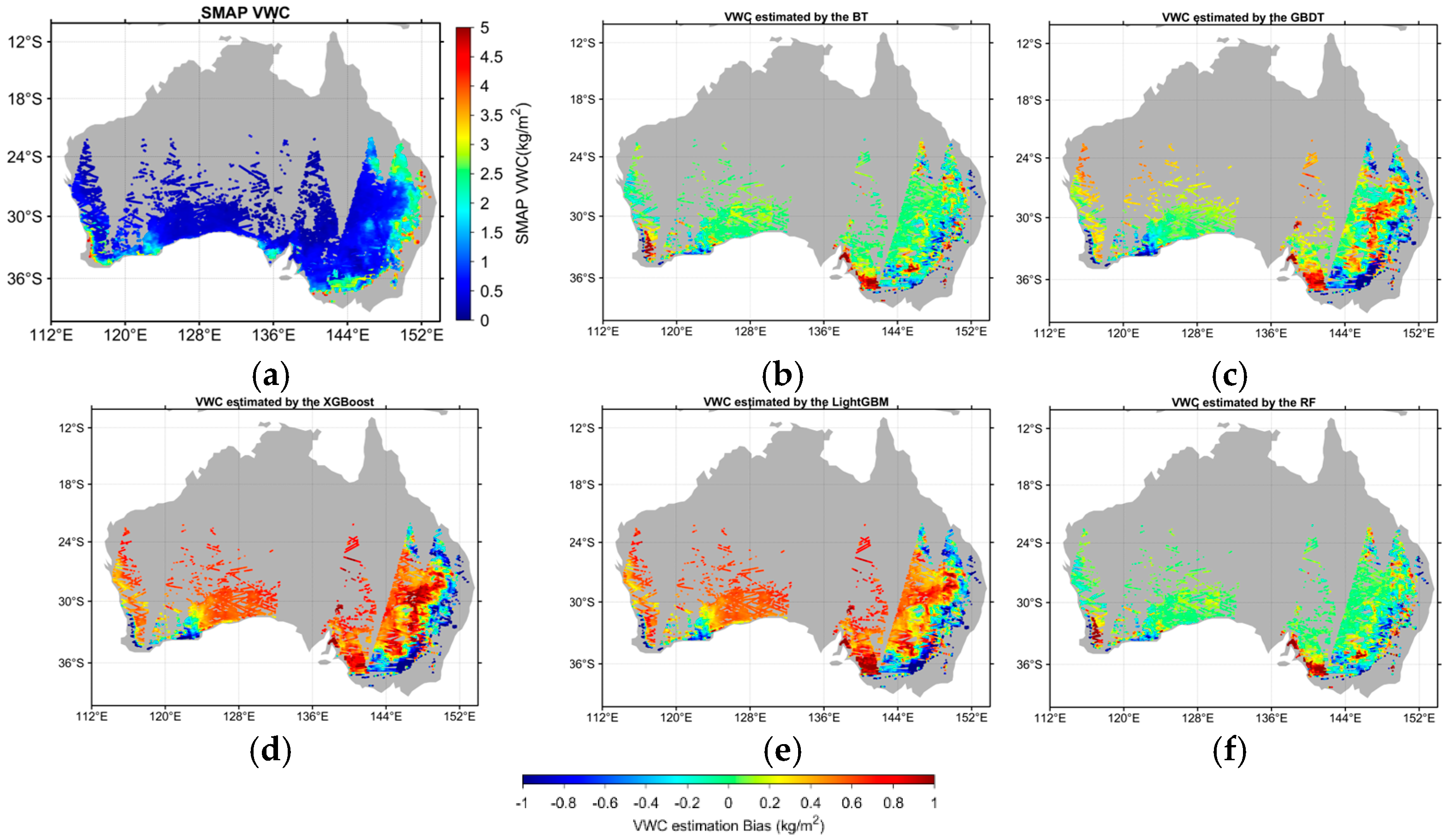
To evaluate the performance of the five proposed models in estimating VWC, we adopted a local analysis approach and selected Australia as the research area. This is an area with rich ecosystems and diverse vegetation types, and most importantly, using Australia, a country dominated by arid and semi-arid regions, can reduce the impact of precipitation and other factors on VWC research. The local deviation distribution between the estimated VWC and SMAP VWC of the five models is depicted in Figure 5. From the graph, we can see that the error distribution of VWC retrieved by BT, GBDT, and RF models is relatively consistent. The areas with larger errors are concentrated in the southeast and southwest of Australia, while the areas with smaller errors are distributed in the central part of Australia. Moreover, we can see that the error between the estimated VWC and SMAP VWC of the BT and RF models is smaller, while the error between the estimated VWC and SMAP VWC of the XGBoost and LightGBM models is larger. To further validate, Figure 6 presents deviation distribution histograms for the five models in estimating VWC against SMAP VWC, displaying mean bias (μ), standard deviation (σ), MAE, and 80% quantile of the bias (Qua). From the graph, it can be seen that this is consistent with the above conclusion, but it is worth noting that all the models displayed underestimation due to model bias or overfitting. Simultaneously, to validate the method’s broad applicability, we chose southeast South America and southeast Africa for verification, as depicted in Figures S1 and S2 in the Supplementary Materials. The findings corroborate those mentioned above.

4.3. Discussion

4.3.1. Performance Using Different Input Strategies

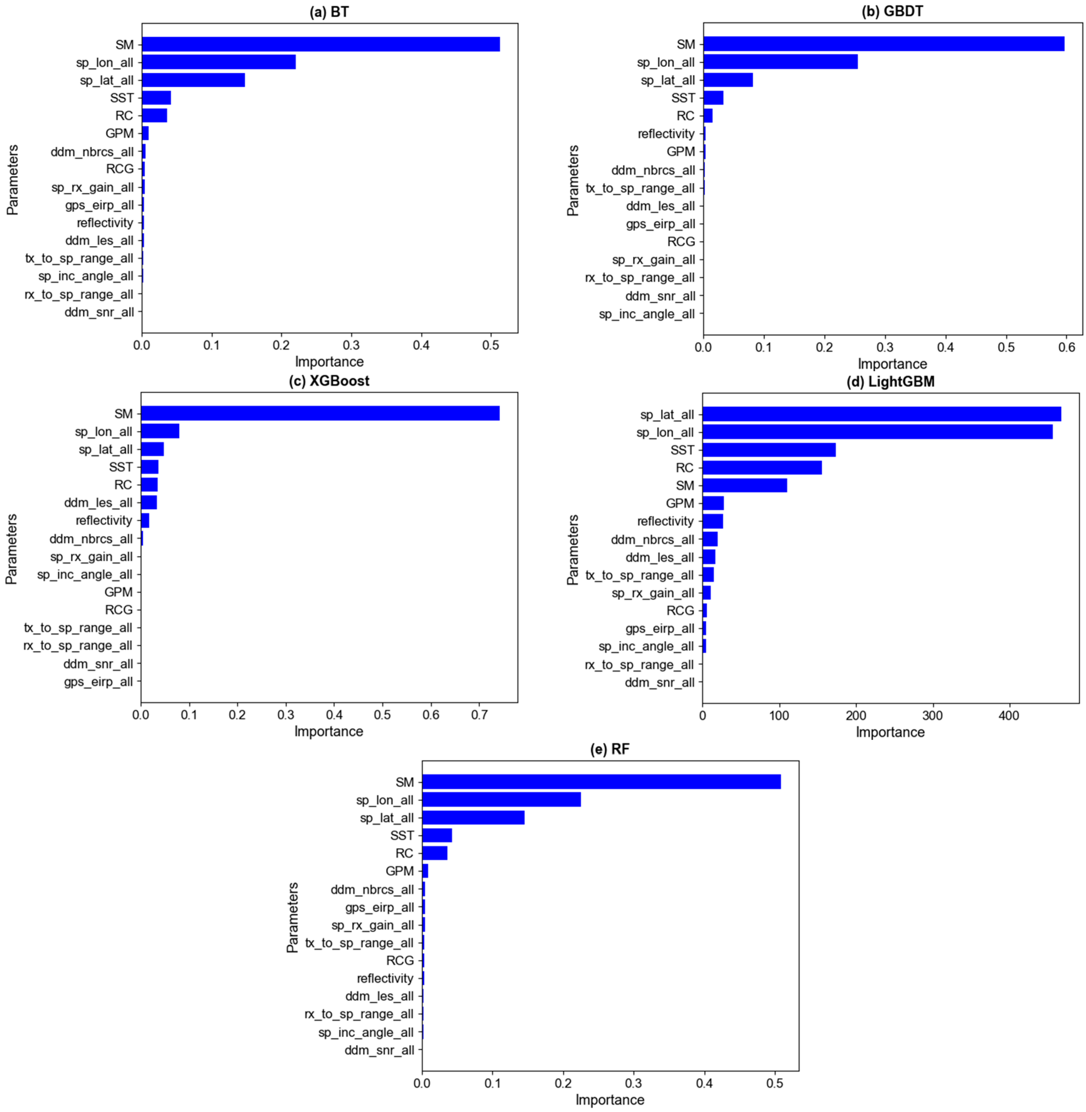
We analyzed the importance of each input feature for five models (i.e., BT, GBDT, XGBoost, RF, and LightGBM). Figure 7 shows the importance ranking of different input variables in estimating VWC. Obviously, we observed that the importance ranking of input variables was not exactly the same across these models, but overall, SM, longitude and latitude of specular point (SP), SST, RC, GPM, reflectivity, NBRCS, and LES are the most important parameters. It should be noted that the feature importance of LightGBM is calculated based on the splitting gain and can give a larger value, while for other models it is calculated based on the Gini coefficient. Therefore, only the importance of input features for the VWC estimation model is provided here.
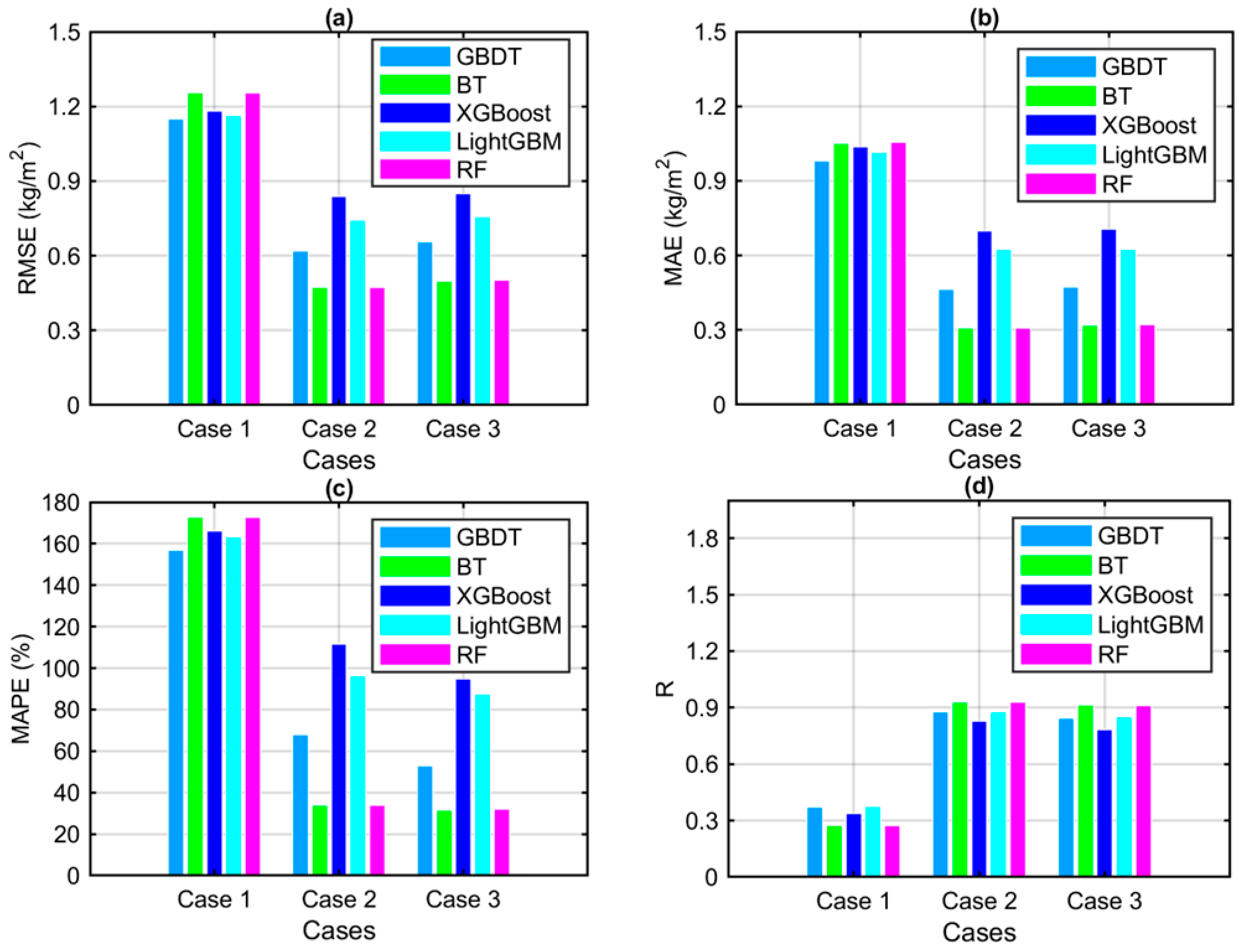
In order to explore the optimal input parameters suitable for the VWC retrieval model, we explore the effects of three different combinations of spaceborne CYGNSS variables and surface auxiliary parameters on the performance of the model. The retrieval models are trained on the same training dataset and tested using the same test set. The different strategies for combining the input parameters of the model are given below.
Case 1: reflectivity, SNR, NBRCS, LES.
Case 2: reflectivity, SNR, NBRCS, LES, incident angle, longitude and latitude of SP, sp_rx_gain, RCG, EIRP.
Case 3: reflectivity, SNR, NBRCS, LES, incident angle, longitude and latitude of SP, sp_rx_gain, RCG, EIRP, precipitation, SM, SST, RC.
We first discuss the effect of the GNSS-R variables on the models, since these parameters are usually the basic configuration used to retrieve VWC, and then consider the effect of adding different surface auxiliary parameters. The performance evaluation of different combination strategies on five models is given in Figure 8, from which it can be seen that the GNSS-R variables are of great help in improving the performance of the models, along with the following observations.
(1)
The position information of the SP, incidence angle, receiver antenna gain, RCG, and ERIP contribute to the retrieval of VWC (Case 1, Case 2). The RMSE of the corresponding five models in Case 2 is decreased by 46.19%, 62.42%, 29.05%, 36.16%, and 62.37%, respectively, compared to Case 1; MAE is decreased by 52.88%, 70.71%, 32.59%, 38.57%, and 70.80%, respectively; MAPE is decreased by 56.71%, 80.39%, 32.98%, 40.99%, and 80.31%, respectively. This improvement is clearly reasonable, and similar to some other studies on the retrieval of geophysical parameters from spaceborne GNSS-R. GNSS-R variables have a positive impact on improving the retrieval performance of geophysical parameters (e.g., SM) [49,77].
(2)
In addition to the GNSS-R variables, four surface auxiliary parameters (precipitation, SM, SST, and RC) were entered into five models in Case 3. We find that these four parameters have little effect on improving the accuracy of the model. Only the MAPE values of the five models are decreased by 22.24%, 7.05%, 14.88%, 9.27%, and 5.71%, respectively.

4.3.2. Cross-Validation Performance in Different Seasons

This subsection further explores the possible effects of seasonal variations on the retrieval of VWC using four quarters of test data in 2021.We divide the test dataset into four test datasets: spring (March–May), summer (June–August), autumn (September–November), and winter (December–February). These subsets are then entered into the five models for computation. The comparison results of CYGNSS retrieval for VWC and SMAP VWC are shown in Figure 9, from which a certain retrieval difference is seen across the four quarters. Overall, the retrieval results for spring and winter were better, while the results for summer were poorer. On the one hand, this may be due to the fact that vegetation starts to grow and germinate in spring and becomes lush in summer, which is accompanied by an increase in VWC, leading to weakened microwave signals due to attenuation. As autumn and winter approach, the evapotranspiration of the plants gradually decreases with the drop in temperature and reduced light hours, causing continuous decrease in the VWC of wilting plants. Similarly, as a mild winter climate brings a new growing season for the vegetation, an increase in VWC appears again, which is consistent with the results in [26].
The RMSE, MAE, MAPE, and R values of the five models in retrieving the VWC for the four seasons are given in Table 5, from which it can be seen that there are some deviation in the retrieval performance of different models in different seasons.
(1)
In spring, the GBDT model had the best retrieval performance for VWC, while the other models show a VWC retrieval performance of LightGBM > XGBoost > BT > RF. In terms of RMSE, the GBDT model improved the retrieval accuracy of VWC by 11.71%, 14.35%, 43.33%, and 46.15% compared to the LightGBM, XGBoost, BT and RF methods, respectively. In terms of MAE, the accuracy was improved by 13.11%, 10.96%, 32.97%, and 35.28%, respectively. In terms of MAPE, the accuracy was improved by 17.38%, 14.60%, 39.33%, and 41.98%, respectively. In terms of R value, the accuracy was improved by 2.89%, 3.91%, 12.75%, and 13.41%, respectively.
(2)
In summer, VWC retrieval performance was best for the RF model, followed by BT > LightGBM > GBDT > XGBoost, The RF model improved the accuracy in terms of RMSE by 1.04%, 2.67%, 9.27%, and 11.72% compared to the BT, LightGBM, GBDT and XGBoost models, respectively. In terms of R value, the accuracy improved by 0.26%, 1.64%, 3.67%, and 3.95%, respectively. In terms of MAE, the accuracy improved by 3.72%, and 9.66% and 11.21% compared to the LightGBM, GBDT and XGBoost models, respectively. In the autumn, the best VWC retrieval performance was achieved by the LightGBM model, followed by BT > XGBoost > RF > GBDT. The accuracy of the LightGBM model compared to the BT, XGBoost, RF, and GBDT models in terms of RMSE improved by 4.52%, 4.56%, 6.96%, and 29.14% respectively. In terms of R value, the accuracy was improved by 0.79%, 1.45%, 1.56%, and 10.78%, respectively. In terms of MAE, the accuracy was improved by 4.25%, 1.97%, and 31.27%, respectively, compared to XGBoost, RF, and GBDT.
(3)
In winter, the VWC retrieval performance showed LightGBM > XGBoost > GBDT > BT > RF, and the LightGBM model improved the accuracy in terms of RMSE by 9.34%, 15.03%, 18.01%, and 18.84% compared to the XGBoost, GBDT, BT, and RF models, respectively. In terms of MAE, the accuracy was improved by 8.83%, 21.80%, 14.35% and 16.02%, respectively. In terms of MAPE, the accuracy was improved by 8.22%, 40.19%, 13.18%, and 14.51%, respectively. In terms of R value, the accuracy was improved by 2.60%, 4.07%, 4.43%, and 4.64%, respectively.
The analysis above illustrates the differences in the generalization ability of different models over different seasons. This indicates that the variation in bias is due to actual VWC seasonal variations, and therefore seasonal parameters should be considered during the construction of VWC retrieval models to improve the performance of CYGNSS VWC retrieval.

4.3.3. Spatial Variations

The effect of seasonal variations on the accuracy of retrieved VWC was discussed above, and in this section, we further discuss the performance of VWC model retrieval at different spatial scales and categorize the study area into low latitude (−10° to 10°), mid-latitude (10° to 30° and −10° to −30°) and high latitude (30° to 40°, −30° to −40°). Figure 10 illustrates the retrieval results of different models across these latitudes. In Figure 10, it is evident that the retrieval performance of the VWC model at different spatial variations shows high latitude > low latitude > mid-latitude, and the main reason for the better performance of the retrieval at high latitudes may be that high latitudes usually have fewer vegetation types and relatively lower vegetation densities, which have more pronounced seasonal variations, and these factors help to improve the performance of the retrieval for VWC, which is consistent with that of the retrieval for different degrees of vegetation cover, as discussed below. Conversely, low-latitude and mid-latitude regions typically feature a greater variety of vegetation types and denser vegetation, which increases signal scattering and absorption. Consequently, the retrieval process becomes more complex in these areas.
Furthermore, Figure 10 reveals that the BT model has the best retrieval performance at low latitudes, followed by the RF model and the XGBoost model, while the GBDT model exhibits the poorest retrieval performance. At mid-latitudes, the RF model performs best, followed by the BT model and the XGBoost model. The worst remains the GBDT model, while at high latitudes, the best retrieval performance is with XGBoost, followed by RF, BT, LightGBM, and GBDT.

4.3.4. Performance Comparison of Different Degrees of Vegetation Coverage

Vegetation coverage is one of the indicators for evaluating the condition of surface vegetation. In general, NDVI, vegetation coverage rate, and vegetation density indicators can be used to evaluate low, medium, and high vegetation coverage. In this article, we use NDVI indicators to divide vegetation coverage into three categories—low, medium, and high vegetation coverage—and verify their performance. Specifically, NDVI was used to define low, medium, and high vegetation cover, and we defined NDVI < 0.25 as low vegetation cover, 0.25 < NDVI < 0.5 as medium vegetation cover, and NDVI > 0.5 as high vegetation cover [78]. The results of different models retrieving VWC under these varied vegetation cover conditions are illustrated in Supplementary Material Figure S3, from which it can be seen that the model retrieving VWC under medium vegetation cover has the best performance and the performance of retrieving VWC under dense vegetation is better than that under sparse vegetation. The lower retrieval accuracy observed under dense vegetation conditions, as opposed to medium vegetation cover, may be attributed to the relatively insensitive nature of vegetation parameters to canopy structure, resulting in saturation of sensitivity, and this finding is basically consistent with previous work [79,80]. Alternatively, it can also be considered that with the effect of signal scattering and attenuation (e.g., the rise in VOD), the vegetation coverage increases, and the GNSS reflected signal power decreases, resulting in a reduction in accuracy [81].
Table 6 displays the retrieval performance over various VWC ranges across different vegetation coverage scenarios. Figure 11 illustrates the probability density function (PDF) distribution curves of VWC and SMAP VWC derived from five models for different vegetation coverage types. Analysis of Table 6 and Figure 11 reveals the following.
(1)
In low vegetation cover, the XGBoost model exhibits the highest accuracy in VWC retrieval among the five models, which corresponds to RMSE, MAE, R, and MAPE of 0.16 kg/m2, 0.09 kg/m2, 0.70, and 31.99%, respectively. Conversely, the worst retrieval accuracy is with the RF model, which corresponds to RMSE, MAE, R, and MAPE of 0.20 kg/m2, 0.11 kg/m2, 0.54, and 37.88%, respectively.
(2)
In medium vegetation cover, the RF model shows the best accuracy in retrieving VWC among the five models, with corresponding RMSE, MAE, R, and MAPE of 0.44 kg/m2, 0.28 kg/m2, 0.81, and 31.93%, respectively. The GBDT model has the worst retrieval performance, which is consistent with sparse vegetation. Its corresponding RMSE, MAE, R, and MAPE are 0.48 kg/m2, 0.36 kg/m2, 0.77, and 44.94%, respectively. The high MAPE values can be attributed to the model’s tendency to overestimate VWC in this range.
(3)
In high vegetation cover, among the models evaluated, the BT and RF models exhibit the most favorable retrieval performance, demonstrating R values of 0.84. Conversely, the GBDT model consistently displays the poorest retrieval performance, yielding R values of 0.71.
It is noteworthy that the PDF of BT and RF models on sparse, moderate, and dense vegetation areas have better agreement with SMAP than the other three models (XGBoost, LightGBM, and GBDT), while GBDT has the worst agreement. This indicates that the BT and RF models have superior retrieval performance for retrieval of VWC for different vegetation cover levels.
The latest CYGNSS-L1-V3.2 version data can be used for research and further optimization of the model framework to reduce dependence on auxiliary data, thereby simplifying model complexity while maximizing model retrieval performance. In addition, the release of more RS data focusing on VWC retrieval will provide more datasets from which to choose (e.g., satellite imagery RS data [14], ALOS-2 PALSAR-2 data [82], and AMSR2 [12], etc.).The cross-validation of CYGNSS retrieved VWC with these datasets, and the fusion of multi-source RS data to obtain monitoring results of vegetation parameters with higher spatial and temporal resolution must be the focus of future research.

5. Conclusions

This study utilizes five ML algorithms to integrate the BRCS, effective scattering area, CYGNSS variables, and surface auxiliary parameters to construct the first localized high-temporal and high-spatial-resolution spaceborne GNSS-R VWC retrieval model. Extensive testing of the different models revealed that the RF and BT models achieve better retrieval performance by comparing them with the SMAP data. Specifically, the RF and BT models exhibited R of 0.91, with only a 1.75% difference in MAPE. The local deviation in the retrieved VWC of the two models was more consistent with the reference value of SMAP. In addition, the inputs of the position information of the SP, incidence angle, receiver antenna gain, RCG, and EIRP contributed to VWC retrieval accuracy.
In order to demonstrate the VWC retrieval capability of the spaceborne GNSS-R across varied conditions, we analyzed different seasons, different spatial scales, and different vegetation cover information, and the results show that the consideration of seasonal parameters improves the accuracy of the CYGNSS VWC retrieval. The performance at high latitudes is better than that at low latitudes and mid-latitudes. The best performance is obtained under medium vegetation cover, while the performance under high vegetation coverage is better than that for sparse vegetation. This provides a useful reference for the retrieval algorithm of VWC in land spaceborne GNSS-R.
Although this article excludes the influence of inland open water bodies on VWC retrieval, it is difficult to completely eliminate errors in inland open water bodies due to data resolution limitations. Therefore, in future work, we will further consider improving the algorithm for eliminating inland open water bodies and consider the impact of terrain errors and other factors on scattering signals. In addition, the estimation of VWC is also affected by factors such as SM, different incidence angles, different polarization modes, vegetation attenuation, etc., and we will further consider eliminating the effects of these factors, improving the spatial and temporal resolution by optimally fusing the CYGNSS and multi-source RS data (SMAP data, AMSR2 data, and ALOS-2 PALSAR-2 data, etc.), and further reduce the model’s dependence on auxiliary data. At the same time, we will consider increasing the number of training datasets by using years of data for training to improve the accuracy of model retrieval. It is more important to integrate multi-frequency, multi-polarization, and multi-system (e.g., CYGNSS/FY-3E/TDS-1/BuFeng-1) satellite GNSS-R data to construct a high-spatiotemporal-resolution VWC retrieval model.

Supplementary Materials

The following supporting information can be downloaded at https://www.mdpi.com/article/10.3390/rs16152793/s1, Figure S1: SMAP VWC (a) and the distribution of local bias (southeastern regions of South America) between SMAP VWC and the estimated VWC of five models: (b) BT; (c) GBDT; (d) XGBoost; (e) LightGBM; (f) RF.; Figure S2: SMAP VWC (a) and the distribution of local bias (southeastern Africa, and Madagascar) between SMAP VWC and the estimated VWC of five models: (b) BT; (c) GBDT; (d) XGBoost; (e) LightGBM; (f) RF; Figure S3: Retrieval results of VWC using different models under different degrees of vegetation coverage: (a–e) sparse vegetation; (f–j) moderate coverage; (k–o) dense vegetation.

Author Contributions

All authors have made significant contributions to this manuscript. Y.Z.: designed the improved method, analyzed the data, wrote the initial version of paper, validated the improved method. J.B.: methodology, writing—review and editing, provided supervision. X.Z.: checked and revised. K.Y.: checked and revised. Q.W.: analyzed the data, checked and revised. W.H.: checked and revised. All authors have read and agreed to the published version of the manuscript.

Funding

This work was supported in part by the Yunnan Fundamental Research Projects under grant 202401CF070151; National Natural Science Foundation of China under grants 42161067 and 42174022; Major scientific and technological projects of Yunnan Province under grant 202202AD080010.

Data Availability Statement

Data is contained within the article or Supplementary Materials.

Acknowledgments

We would like to thank NASA for providing CYGNSS data, the European Center for Medium-Range Weather Forecasts (ECMWF) for providing the surface temperature data, and the developers of SMAP, MODIS, AMSRU, Global Surface Water (GSW), and IMERG products for providing the data freely available to the public. The authors also thank the anonymous reviewers for their in-depth reviews and helpful suggestions that have largely contributed to improving this paper.

Conflicts of Interest

The authors declare no conflicts of interest.

References

  1. Konings, A.G.; Saatchi, S.S.; Frankenberg, C.; Keller, M.; Leshyk, V.; Anderegg, W.R.L.; Humphrey, V.; Matheny, A.M.; Trugman, A.; Sack, L.; et al. Detecting forest response to droughts with global observations of vegetation water content. Glob. Change Biol. 2021, 27, 6005–6024. [Google Scholar] [CrossRef] [PubMed]
  2. Wang, X.; Zhang, Z.; Lu, S.; Zhen, S.; Zhao, H.; Yin, Y. Combining Microwave and Optical Remote Sensing to Characterize Global Vegetation Water Status. IEEE Trans. Geosci. Remote Sens. 2023, 61, 5301719. [Google Scholar] [CrossRef]
  3. Saeed, F.; Bethke, I.; Fischer, E.; Legutke, S.; Shiogama, H.; Stone, D.A.; Schleussner, C.-F. Robust changes in tropical rainy season length at 1.5 °C and 2 °C. Environ. Res. Lett. 2018, 13, 064024. [Google Scholar] [CrossRef]
  4. Yebra, M.; Scortechini, G.; Badi, A.; Beget, M.E.; Boer, M.M.; Bradstock, R.; Chuvieco, E.; Danson, F.M.; Dennison, P.; Resco de Dios, V.; et al. Globe-LFMC, a global plant water status database for vegetation ecophysiology and wildfire applications. Sci. Data 2019, 6, 155. [Google Scholar] [CrossRef] [PubMed]
  5. Jackson, R.D. Remote Sensing of Biotic and Abiotic Plant Stress. Annu. Rev. Phytopathol. 1986, 24, 265–287. [Google Scholar] [CrossRef]
  6. Doughty, R.; Köhler, P.; Frankenberg, C.; Magney, T.S.; Xiao, X.; Qin, Y.; Wu, X.; Moore, B. TROPOMI reveals dry-season increase of solar-induced chlorophyll fluorescence in the Amazon forest. Proc. Natl. Acad. Sci. USA 2019, 116, 22393–22398. [Google Scholar] [CrossRef]
  7. Brando, P.M.; Goetz, S.J.; Baccini, A.; Nepstad, D.C.; Beck, P.S.A.; Christman, M.C. Seasonal and interannual variability of climate and vegetation indices across the Amazon. Proc. Natl. Acad. Sci. USA 2010, 107, 14685–14690. [Google Scholar] [CrossRef] [PubMed]
  8. Wang, H.; Wigneron, J.-P.; Ciais, P.; Yao, Y.; Fan, L.; Liu, X.; Li, X.; Green, J.K.; Tian, F.; Tao, S.; et al. Seasonal variations in vegetation water content retrieved from microwave remote sensing over Amazon intact forests. Remote Sens. Environ. 2023, 285, 113409. [Google Scholar] [CrossRef]
  9. Ma, S.; Zhou, Y.; Gowda, P.H.; Dong, J.; Zhang, G.; Kakani, V.G.; Wagle, P.; Chen, L.; Flynn, K.C.; Jiang, W. Application of the water-related spectral reflectance indices: A review. Ecol. Indic. 2019, 98, 68–79. [Google Scholar] [CrossRef]
  10. Huang, Y.; Walker, J.P.; Gao, Y.; Wu, X.; Monerris, A. Estimation of Vegetation Water Content From the Radar Vegetation Index at L-Band. IEEE Trans. Geosci. Remote Sens. 2016, 54, 981–989. [Google Scholar] [CrossRef]
  11. Srivastava, P.K.; Neill, P.O.; Cosh, M.; Lang, R.; Joseph, A. Evaluation of radar vegetation indices for vegetation water content estimation using data from a ground-based SMAP simulator. In Proceedings of the 2015 IEEE International Geoscience and Remote Sensing Symposium (IGARSS), Milan, Italy, 26–31 July 2015; pp. 1296–1299. [Google Scholar]
  12. Santi, E.; Paloscia, S.; Pampaloni, P.; Pettinato, S.; Nomaki, T.; Seki, M.; Sekiya, K.; Maeda, T. Vegetation Water Content Retrieval by Means of Multifrequency Microwave Acquisitions From AMSR2. IEEE J. Sel. Top. Appl. Earth Obs. Remote Sens. 2017, 10, 3861–3873. [Google Scholar] [CrossRef]
  13. Entekhabi, D.; Njoku, E.G.; Neill, P.E.O.; Kellogg, K.H.; Crow, W.T.; Edelstein, W.N.; Entin, J.K.; Goodman, S.D.; Jackson, T.J.; Johnson, J.; et al. The Soil Moisture Active Passive (SMAP) Mission. Proc. IEEE 2010, 98, 704–716. [Google Scholar] [CrossRef]
  14. Wang, Q.; Chai, L.; Zhao, S.; Zhang, Z. Gravimetric Vegetation Water Content Estimation for Corn Using L-Band Bi-Angular, Dual-Polarized Brightness Temperatures and Leaf Area Index. Remote Sens. 2015, 7, 10543–10561. [Google Scholar] [CrossRef]
  15. Zavorotny, V.U.; Gleason, S.; Cardellach, E.; Camps, A. Tutorial on Remote Sensing Using GNSS Bistatic Radar of Opportunity. IEEE Geosci. Remote Sens. Mag. 2014, 2, 8–45. [Google Scholar] [CrossRef]
  16. Cygnss. CYGNSS Level 1 Science Data Record Version 3.0. 2020. Available online: https://catalog.data.gov/dataset/cygnss-level-1-science-data-record-version-3-0-340fb (accessed on 25 February 2024).
  17. Yan, Q.; Huang, W.; Jin, S.; Jia, Y. Pan-tropical soil moisture mapping based on a three-layer model from CYGNSS GNSS-R data. Remote Sens. Environ. 2020, 247, 111944. [Google Scholar] [CrossRef]
  18. Shi, Y.; Liang, Y.; Ren, C.; Lai, J.; Ding, Q.; Hu, X. Investigating the Effects of Meteorological Data Rainfall and Temperature on GNSS-R Soil Moisture Inversion. In Proceedings of the 2021 IEEE Specialist Meeting on Reflectometry Using GNSS and Other Signals of Opportunity (GNSS+R), Virtual, 14–17 September 2021; pp. 97–100. [Google Scholar]
  19. Bu, J.; Yu, K.; Zuo, X.; Ni, J.; Li, Y.; Huang, W. GloWS-Net: A Deep Learning Framework for Retrieving Global Sea Surface Wind Speed Using Spaceborne GNSS-R Data. Remote Sens. 2023, 15, 590. [Google Scholar] [CrossRef]
  20. Bu, J.; Yu, K.; Ni, J.; Huang, W. Combining ERA5 data and CYGNSS observations for the joint retrieval of global significant wave height of ocean swell and wind wave: A deep convolutional neural network approach. J. Geod. 2023, 97, 81. [Google Scholar] [CrossRef]
  21. Komjathy, A.; Maslanik, J.; Zavorotny, V.U.; Axelrad, P.; Katzberg, S.J. Sea ice remote sensing using surface reflected GPS signals. In Proceedings of the IGARSS 2000. IEEE 2000 International Geoscience and Remote Sensing Symposium. Taking the Pulse of the Planet: The Role of Remote Sensing in Managing the Environment. Proceedings (Cat. No.00CH37120), Honolulu, HI, USA, 24–28 July 2000; Volume 2857, pp. 2855–2857. [Google Scholar]
  22. Yan, Q.; Huang, W. Spaceborne GNSS-R Sea Ice Detection Using Delay-Doppler Maps: First Results From the U.K. TechDemoSat-1 Mission. IEEE J. Sel. Top. Appl. Earth Obs. Remote Sens. 2016, 9, 4795–4801. [Google Scholar] [CrossRef]
  23. Larson, K.M.; Ray, R.D.; Nievinski, F.G.; Freymueller, J.T. The Accidental Tide Gauge: A GPS Reflection Case Study From Kachemak Bay, Alaska. IEEE Geosci. Remote Sens. Lett. 2013, 10, 1200–1204. [Google Scholar] [CrossRef]
  24. Cardellach, E.; Fabra, F.; Rius, A.; Pettinato, S.; D’Addio, S. Characterization of dry-snow sub-structure using GNSS reflected signals. Remote Sens. Environ. 2012, 124, 122–134. [Google Scholar] [CrossRef]
  25. Yan, Q.; Liu, S.; Chen, T.; Jin, S.; Xie, T.; Huang, W. Mapping Surface Water Fraction Over the Pan-Tropical Region Using CYGNSS Data. IEEE Trans. Geosci. Remote Sens. 2024, 62, 1–14. [Google Scholar] [CrossRef]
  26. Li, S.; Jing, H.; Yuan, Q.; Yue, L.; Li, T. Investigating the spatio-temporal variation of vegetation water content in the western United States by blending GNSS-IR, AMSR-E, and AMSR2 observables using machine learning methods. Sci. Remote Sens. 2022, 6, 100061. [Google Scholar] [CrossRef]
  27. Loria, E.; O’Brien, A.; Zavorotny, V.; Lavalle, M.; Chew, C.; Shah, R.; Zuffada, C. Analysis of Wetland Extent Retrieval Accuracy Using Cygnss. In Proceedings of the IGARSS 2019—2019 IEEE International Geoscience and Remote Sensing Symposium, Yokohama, Japan, 28 July–2 August 2019; pp. 8684–8687. [Google Scholar]
  28. Chew, C.; Small, E.E.; Larson, K.M. An algorithm for soil moisture estimation using GPS-interferometric reflectometry for bare and vegetated soil. GPS Solut. 2016, 20, 525–537. [Google Scholar] [CrossRef]
  29. Rodriguez-Alvarez, N.; Bosch-Lluis, X.; Camps, A.; Ramos-Perez, I.; Valencia, E.; Park, H.; Vall-llossera, M. Vegetation Water Content Estimation Using GNSS Measurements. IEEE Geosci. Remote Sens. Lett. 2012, 9, 282–286. [Google Scholar] [CrossRef]
  30. Rodriguez-Alvarez, N.; Camps, A.; Vall-llossera, M.; Bosch-Lluis, X.; Monerris, A.; Ramos-Perez, I.; Valencia, E.; Marchan-Hernandez, J.F.; Martinez-Fernandez, J.; Baroncini-Turricchia, G.; et al. Land Geophysical Parameters Retrieval Using the Interference Pattern GNSS-R Technique. IEEE Trans. Geosci. Remote Sens. 2011, 49, 71–84. [Google Scholar] [CrossRef]
  31. Pierdicca, N.; Guerriero, L.; Caparrini, M.; Egido, A.; Paloscia, S.; Santi, E.; Floury, N. GNSS Reflectometry as a tool to retrieve soil moisture and vegetation biomass: Experimental and theoretical activities. In Proceedings of the 2013 International Conference on Localization and GNSS (ICL-GNSS), Turin, Italy, 25–27 June 2013; pp. 1–5. [Google Scholar]
  32. Egido, A.; Paloscia, S.; Motte, E.; Guerriero, L.; Pierdicca, N.; Caparrini, M.; Santi, E.; Fontanelli, G.; Floury, N. Airborne GNSS-R Polarimetric Measurements for Soil Moisture and Above-Ground Biomass Estimation. IEEE J. Sel. Top. Appl. Earth Obs. Remote Sens. 2014, 7, 1522–1532. [Google Scholar] [CrossRef]
  33. Motte, E.; Fanise, P.; Zribi, M. GLORI (GLObal navigation satellite system Reflectometry Instrument). In Proceedings of the 2015 IEEE International Geoscience and Remote Sensing Symposium (IGARSS), Milan, Italy, 26–31 July 2015; pp. 4773–4776. [Google Scholar]
  34. Zribi, M.; Matte, E.; Fanise, P.; Guyon, D.; Wigneron, J.P.; Baghdadi, N.; Pierdicca, N. Performances of GNSS-R Glori Data Over Lande Forest. In Proceedings of the IGARSS 2018—2018 IEEE International Geoscience and Remote Sensing Symposium, Valencia, Spain, 22–27 July 2018; pp. 2039–2042. [Google Scholar]
  35. Jia, Y.; Savi, P. Polarimetric GNSS-R measurements for soil moisture and vegetation sensing. In Proceedings of the 2016 IEEE International Geoscience and Remote Sensing Symposium (IGARSS), Beijing, China, 10–15 July 2016; pp. 5260–5263. [Google Scholar]
  36. Park, H.; Camps, A.; Castellvi, J.; Muro, J. Generic Performance Simulator of Spaceborne GNSS-Reflectometer for Land Applications. IEEE J. Sel. Top. Appl. Earth Obs. Remote Sens. 2020, 13, 3179–3191. [Google Scholar] [CrossRef]
  37. Munoz-Martin, J.F.; Pascual, D.; Onrubia, R.; Park, H.; Camps, A.; Rüdiger, C.; Walker, J.P.; Monerris, A. Vegetation Canopy Height Retrieval Using L1 and L5 Airborne GNSS-R. IEEE Geosci. Remote Sens. Lett. 2022, 19, 2502405. [Google Scholar] [CrossRef]
  38. Wu, X.; Guo, P.; Sun, Y.; Liang, H.; Zhang, X.; Bai, W. Recent Progress on Vegetation Remote Sensing Using Spaceborne GNSS-Reflectometry. Remote Sens. 2021, 13, 4244. [Google Scholar] [CrossRef]
  39. Bu, J.; Wang, Q.; Wang, Z.; Fan, S.; Liu, X.; Zuo, X. Land Remote Sensing Applications Using Spaceborne GNSS Reflectometry: A Comprehensive Overview. IEEE J. Sel. Top. Appl. Earth Obs. Remote Sens. 2024, 17, 12811–12841. [Google Scholar] [CrossRef]
  40. Ferrazzoli, P.; Guerriero, L.; Pierdicca, N.; Rahmoune, R. Forest biomass monitoring with GNSS-R: Theoretical simulations. Adv. Space Res. 2011, 47, 1823–1832. [Google Scholar] [CrossRef]
  41. Camps, A.; Park, H.; Pablos, M.; Foti, G.; Gommenginger, C.P.; Liu, P.W.; Judge, J. Sensitivity of GNSS-R Spaceborne Observations to Soil Moisture and Vegetation. IEEE J. Sel. Top. Appl. Earth Obs. Remote Sens. 2016, 9, 4730–4742. [Google Scholar] [CrossRef]
  42. Carreno-Luengo, H.; Lowe, S.; Zuffada, C.; Esterhuizen, S.; Oveisgharan, S. Spaceborne GNSS-R from the SMAP Mission: First Assessment of Polarimetric Scatterometry over Land and Cryosphere. Remote Sens. 2017, 9, 362. [Google Scholar] [CrossRef]
  43. Santi, E.; Clarizia, M.P.; Comite, D.; Dente, L.; Guerriero, L.; Pierdicca, N.; Floury, N. Combining Cygnss and Machine Learning for Soil Moisture and Forest Biomass Retrieval in View of the ESA Scout Hydrognss Mission. In Proceedings of the IGARSS 2022—2022 IEEE International Geoscience and Remote Sensing Symposium, Kuala Lumpur, Malaysia, 17–22 July 2022; pp. 7433–7436. [Google Scholar]
  44. Santi, E.; Pettinato, S.; Paloscia, S.; Clarizia, M.P.; Dente, L.; Guerriero, L.; Comite, D.; Pierdicca, N. Soil Moisture and Forest Biomass retrieval on a global scale by using CyGNSS data and Artificial Neural Networks. In Proceedings of the IGARSS 2020—2020 IEEE International Geoscience and Remote Sensing Symposium, Virtual, 26 September–2 October 2020; pp. 5905–5908. [Google Scholar]
  45. Carreno-Luengo, H.; Luzi, G.; Crosetto, M. Above-Ground Biomass Retrieval over Tropical Forests: A Novel GNSS-R Approach with CyGNSS. Remote Sens. 2020, 12, 1368. [Google Scholar] [CrossRef]
  46. Santi, E.; Paloscia, S.; Pettinato, S.; Fontanelli, G.; Clarizia, M.P.; Comite, D.; Dente, L.; Guerriero, L.; Pierdicca, N.; Floury, N. Remote Sensing of Forest Biomass Using GNSS Reflectometry. IEEE J. Sel. Top. Appl. Earth Obs. Remote Sens. 2020, 13, 2351–2368. [Google Scholar] [CrossRef]
  47. Pilikos, G.; Clarizia, M.P.; Floury, N. Biomass Estimation with GNSS Reflectometry Using a Deep Learning Retrieval Model. Remote Sens. 2024, 16, 1125. [Google Scholar] [CrossRef]
  48. Chen, F.; Liu, L.; Guo, F.; Huang, L. A New Vegetation Observable Derived from Spaceborne GNSS-R and Its Application to Vegetation Water Content Retrieval. Remote Sens. 2024, 16, 931. [Google Scholar] [CrossRef]
  49. Nabi, M.M.; Senyurek, V.; Gurbuz, A.C.; Kurum, M. Deep Learning-Based Soil Moisture Retrieval in CONUS Using CYGNSS Delay–Doppler Maps. IEEE J. Sel. Top. Appl. Earth Obs. Remote Sens. 2022, 15, 6867–6881. [Google Scholar] [CrossRef]
  50. Al-Khaldi, M.M.; Johnson, J.T.; Gleason, S.; Loria, E.; O’Brien, A.J.; Yi, Y. An algorithm for detecting coherence in cyclone global navigation satellite system mission level-1 delay-Doppler maps. IEEE Trans. Geosci. Remote Sens. 2020, 59, 4454–4463. [Google Scholar] [CrossRef]
  51. Jia, Y.; Jin, S.; Savi, P.; Yan, Q.; Li, W. Modeling and theoretical analysis of GNSS-R soil moisture retrieval based on the random forest and support vector machine learning approach. Remote Sens. 2020, 12, 3679. [Google Scholar] [CrossRef]
  52. Yan, Q.; Gong, S.; Jin, S.; Huang, W.; Zhang, C. Near real-time soil moisture in China retrieved from CyGNSS reflectivity. IEEE Geosci. Remote Sens. Lett. 2020, 19, 1–5. [Google Scholar] [CrossRef]
  53. O’Neill, P.; Chan, S.; Njoku, E.G.; Jackson, T.; Bindlish, R.; Chaubell, J.; Colliander, A. SMAP enhanced L3 radiometer global and polar grid daily 9 km ease-grid soil moisture version 5. Natl. Snow Ice Data Cent. 2021. [Google Scholar] [CrossRef]
  54. Huffman, G.; Stocker, E.; Bolvin, D.; Nelkin, E.; Tan, J. GPM IMERG late precipitation L3 1 day 0.1 degree × 0.1 degree V05, Edited by Andrey Savtchenko, Greenbelt, MD Goddard Earth Sci. Data Inf. Serv. Cent. 2016. [Google Scholar] [CrossRef]
  55. Muñoz Sabater, J. ERA5-Land Hourly Data from 1981 to Present. Copernicus Climate Change Service (C3S) Climate Data Store (CDS). 2019, Volume 10. Available online: https://cds.climate.copernicus.eu/cdsapp#!/dataset/10.24381/cds.e2161bac?tab=overview (accessed on 25 February 2024).
  56. Friedl, M.; Sulla-Menashe, D. MODIS/Terra+ Aqua Land Cover Type Yearly L3 Global 500m SIN Grid V061. NASA EOSDIS Land Processes DAAC. 2022. Available online: https://lpdaac.usgs.gov/products/mcd12c1v061/ (accessed on 26 February 2024).
  57. Du, J.; Kimball, J.S.; Jones, L.A.; Kim, Y.; Glassy, J.; Watts, J.D. A global satellite environmental data record derived from AMSR-E and AMSR2 microwave Earth observations. Earth Syst. Sci. Data 2017, 9, 791–808. [Google Scholar] [CrossRef]
  58. Pekel, J.-F.; Cottam, A.; Gorelick, N.; Belward, A.S. High-resolution mapping of global surface water and its long-term changes. Nature 2016, 540, 418–422. [Google Scholar] [CrossRef] [PubMed]
  59. Cook, B.I.; Smerdon, J.E.; Seager, R.; Coats, S. Global warming and 21st century drying. Clim. Dyn. 2014, 43, 2607–2627. [Google Scholar] [CrossRef]
  60. Zhang, S.; Guo, Q.; Liu, Q.; Ma, Z.; Liu, N.; Hu, S.; Bao, L.; Zhou, X.; Zhao, H.; Wang, L.; et al. Improvement of CYGNSS soil moisture retrieval model considering water and surface temperature. Adv. Space Res. 2023, 72, 3048–3064. [Google Scholar] [CrossRef]
  61. Calvet, J.C.; Wigneron, J.P.; Walker, J.; Karbou, F.; Chanzy, A.; Albergel, C. Sensitivity of Passive Microwave Observations to Soil Moisture and Vegetation Water Content: L-Band to W-Band. IEEE Trans. Geosci. Remote Sens. 2011, 49, 1190–1199. [Google Scholar] [CrossRef]
  62. Zhang, Y.; Zhou, S.; Gentine, P.; Xiao, X. Can vegetation optical depth reflect changes in leaf water potential during soil moisture dry-down events? Remote Sens. Environ. 2019, 234, 111451. [Google Scholar] [CrossRef]
  63. Lei, F.; Senyurek, V.; Kurum, M.; Gurbuz, A.C.; Boyd, D.; Moorhead, R.; Crow, W.T.; Eroglu, O. Quasi-global machine learning-based soil moisture estimates at high spatio-temporal scales using CYGNSS and SMAP observations. Remote Sens. Environ. 2022, 276, 113041. [Google Scholar] [CrossRef]
  64. Senyurek, V.; Lei, F.; Boyd, D.; Kurum, M.; Gurbuz, A.C.; Moorhead, R. Machine Learning-Based CYGNSS Soil Moisture Estimates over ISMN sites in CONUS. Remote Sens. 2020, 12, 1168. [Google Scholar] [CrossRef]
  65. Bu, J.; Yu, K.; Park, H.; Huang, W.; Han, S.; Yan, Q.; Qian, N.; Lin, Y. Estimation of Swell Height Using Spaceborne GNSS-R Data from Eight CYGNSS Satellites. Remote Sens. 2022, 14, 4634. [Google Scholar] [CrossRef]
  66. Al-Khaldi, M.M.; Johnson, J.T.; O’Brien, A.J.; Balenzano, A.; Mattia, F. Time-Series Retrieval of Soil Moisture Using CYGNSS. IEEE Trans. Geosci. Remote Sens. 2019, 57, 4322–4331. [Google Scholar] [CrossRef]
  67. Lu, C.; Wang, Z.; Wu, Z.; Zheng, Y.; Liu, Y. Global Ocean Wind Speed Retrieval From GNSS Reflectometry Using CNN-LSTM Network. IEEE Trans. Geosci. Remote Sens. 2023, 61, 1–12. [Google Scholar] [CrossRef]
  68. Clarizia, M.P.; Pierdicca, N.; Costantini, F.; Floury, N. Analysis of CYGNSS Data for Soil Moisture Retrieval. IEEE J. Sel. Top. Appl. Earth Obs. Remote Sens. 2019, 12, 2227–2235. [Google Scholar] [CrossRef]
  69. Pierdicca, N.; Comite, D.; Camps, A.; Carreno-Luengo, H.; Cenci, L.; Clarizia, M.P.; Costantini, F.; Dente, L.; Guerriero, L.; Mollfulleda, A.; et al. The Potential of Spaceborne GNSS Reflectometry for Soil Moisture, Biomass, and Freeze–Thaw Monitoring: Summary of a European Space Agency-funded study. IEEE Geosci. Remote Sens. Mag. 2022, 10, 8–38. [Google Scholar] [CrossRef]
  70. Wang, B.; Cha, H.; Zhou, Z.; Tian, B. Clutter Cancellation and Long Time Integration for GNSS-Based Passive Bistatic Radar. Remote Sens. 2021, 13, 701. [Google Scholar] [CrossRef]
  71. Wang, C.; Yu, K.; Qu, F.; Bu, J.; Han, S.; Zhang, K. Spaceborne GNSS-R Wind Speed Retrieval Using Machine Learning Methods. Remote Sens. 2022, 14, 3507. [Google Scholar] [CrossRef]
  72. Friedman, J.H. Greedy Function Approximation: A Gradient Boosting Machine. Ann. Stat. 2001, 29, 1189–1232. [Google Scholar] [CrossRef]
  73. Min, X.F.; Wang, A.Q.; Yang, L.X. Parameter Inversion of Rough Surface based on GBDT Model. In Proceedings of the 2022 International Applied Computational Electromagnetics Society Symposium (ACES-China), Xuzhou, China, 9–12 December 2022; pp. 1–2. [Google Scholar]
  74. Prasad, A.M.; Iverson, L.R.; Liaw, A. Newer Classification and Regression Tree Techniques: Bagging and Random Forests for Ecological Prediction. Ecosystems 2006, 9, 181–199. [Google Scholar] [CrossRef]
  75. Wang, C.; Yu, K.; Zhang, K.; Bu, J.; Qu, F. Significant Wave Height Retrieval Based on Multivariable Regression Models Developed With CYGNSS Data. IEEE Trans. Geosci. Remote Sens. 2023, 61, 1–15. [Google Scholar] [CrossRef]
  76. Bu, J.; Yu, K.; Zhu, Y.; Qian, N.; Chang, J. Developing and Testing Models for Sea Surface Wind Speed Estimation with GNSS-R Delay Doppler Maps and Delay Waveforms. Remote Sens. 2020, 12, 3760. [Google Scholar] [CrossRef]
  77. Nabi, M.M.; Senyurek, V.; Lei, F.; Kurum, M.; Gurbuz, A.C. Quasi-Global Assessment of Deep Learning-Based CYGNSS Soil Moisture Retrieval. IEEE J. Sel. Top. Appl. Earth Obs. Remote Sens. 2023, 16, 5629–5644. [Google Scholar] [CrossRef]
  78. Gao, L.; Wang, X.; Johnson, B.A.; Tian, Q.; Wang, Y.; Verrelst, J.; Mu, X.; Gu, X. Remote sensing algorithms for estimation of fractional vegetation cover using pure vegetation index values: A review. ISPRS J. Photogramm. Remote Sens. 2020, 159, 364–377. [Google Scholar] [CrossRef] [PubMed]
  79. Gamon, J.A.; Field, C.B.; Goulden, M.L.; Griffin, K.L.; Hartley, A.E.; Joel, G.; Penuelas, J.; Valentini, R. Relationships Between NDVI, Canopy Structure, and Photosynthesis in Three Californian Vegetation Types. Ecol. Appl. 1995, 5, 28–41. [Google Scholar] [CrossRef]
  80. Kim, S.; Garrison, J.L.; Kurum, M. Retrieval of Subsurface Soil Moisture and Vegetation Water Content From Multifrequency SoOp Reflectometry: Sensitivity Analysis. IEEE Trans. Geosci. Remote Sens. 2023, 61, 1–18. [Google Scholar] [CrossRef]
  81. Zribi, M.; Motte, E.; Baghdadi, N.; Baup, F.; Dayau, S.; Fanise, P.; Guyon, D.; Huc, M.; Wigneron, J.P. Potential Applications of GNSS-R Observations over Agricultural Areas: Results from the GLORI Airborne Campaign. Remote Sens. 2018, 10, 1245. [Google Scholar] [CrossRef]
  82. Zhang, Y.; Ling, F.; Foody, G.M.; Ge, Y.; Boyd, D.S.; Li, X.; Du, Y.; Atkinson, P.M. Mapping annual forest cover by fusing PALSAR/PALSAR-2 and MODIS NDVI during 2007–2016. Remote Sens. Environ. 2019, 224, 74–91. [Google Scholar] [CrossRef]
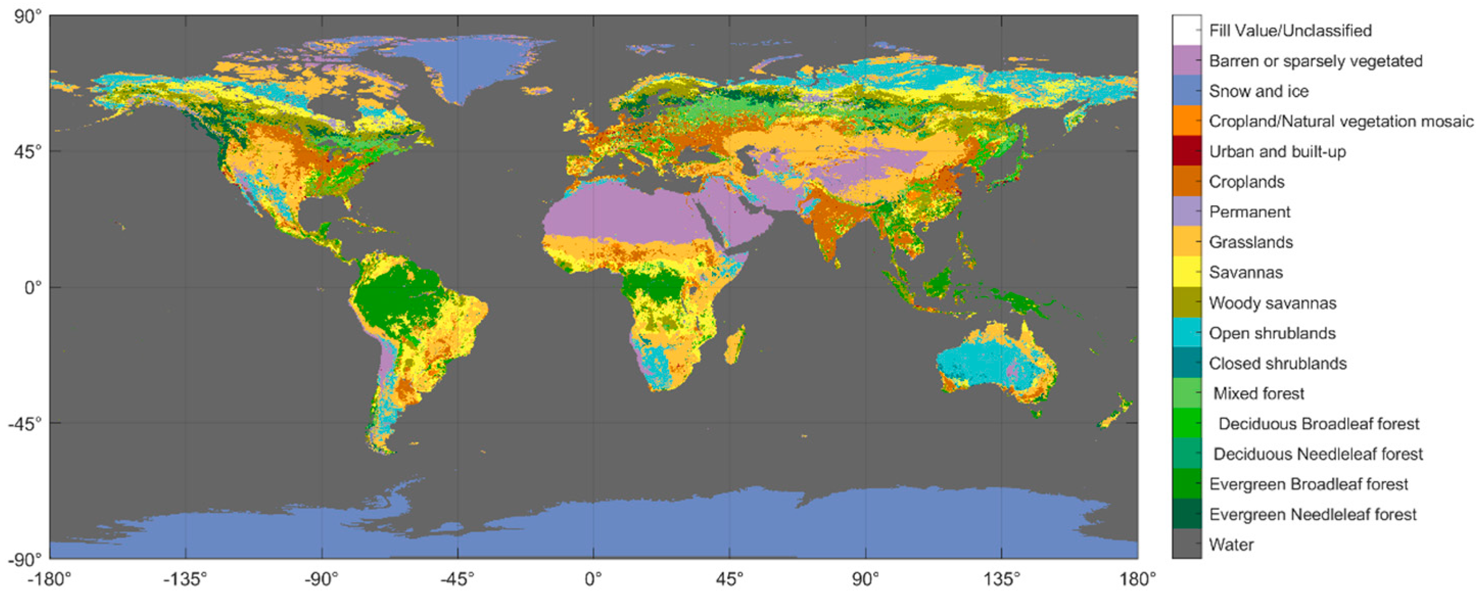
Figure 1. IGBP land classification map (2021 year).
Remotesensing 16 02793 g001
Figure 2. Algorithm flow of bagging tree model algorithm.
Remotesensing 16 02793 g002
Figure 3. Construction and evaluation flow chart of VWC retrieval mode.
Remotesensing 16 02793 g003
Figure 4. Scatter density plots for the retrieval of VWC and SMAP VWC using five models: (a) GBDT; (b) BT; (c) XGBoost; (d) LightGBM; (e) RF.
Remotesensing 16 02793 g004
Figure 5. SMAP VWC (a) and the distribution of local bias (Australia) between SMAP VWC and the estimated VWC of five models: (b) BT; (c) GBDT; (d) XGBoost; (e) LightGBM; (f) RF.
Remotesensing 16 02793 g005
Figure 6. Histograms illustrating the distribution of discrepancies between SMAP VWC and VWC estimated by five models: (a) BT; (b) GBDT; (c) XGBoost; (d) LightGBM; (e) RF.
Remotesensing 16 02793 g006
Figure 7. The importance of 16 indices generated by five models: (a) BT; (b) GBDT; (c) XGBoost; (d) LightGBM; (e) RF.
Remotesensing 16 02793 g007
Figure 8. Performance evaluation of different parameter combination strategies (three schemes) on five models (GBDT, BT, XGBoost, LightGBM, and RF). (a) RMSE; (b) MAE; (c) MAPE; (d) R.
Remotesensing 16 02793 g008
Figure 9. Scatter density plots of VWC and SMAP VWC for four quarters retrieved by five models: (ae) spring; (fj) summer; (ko) autumn; (pt) winter.
Remotesensing 16 02793 g009
Figure 10. VWC retrieval performance of various models at different latitudes: (ae) low latitudes; (fj) mid-latitudes; (ko) high latitudes.
Remotesensing 16 02793 g010
Figure 11. PDF distribution curves of VWC and SMAP VWC retrieved from five models with different vegetation cover: low (a), medium (b), and high (c).
Remotesensing 16 02793 g011
Table 1. Statistical table of the data variables and their sources used in this article.
CategoryDatasetsSpatial ResolutionTime ResolutionParametersReference
CYGNSS L1B dataCYGNSS L1B25 km1 s (sampling point time interval)power_analog, ddm_snr,
ddm_nbrcs, GNSS-R observables, metadata variables
[16]
Reference and validation dataSMAP9 kmdailySM, VWC,
SST, roughness coefficient (RC)
[53]
Auxiliary data for the retrieval processGPM IMERG0.1°dailyprecipitation[54]
ECMWF0.1°hourlySST[55]
MCD12C10.05°yearlydeciduous coniferous forests, water bodies, snow and ice, etc.[56]
AMSRU25 kmdailySM[57]
GSW100 m3 monthsinland water data[58]
Table 2. Quality flags of spaceborne GNSS-R data from CYGNSS.
IndicatorsSetting
s_band_powered_up0
large_sc_attitude_err0
black_body_ddm0
ddmi_reconFigd0
spacewire_crc_invalid0
ddm_is_test_pattern0
channel_idle0
sp_over_land1
direct_signal_in_ddm0
low_confidence_gps_eirp_estimate0
rfi_detected0
sp_non_existent_error0
bb_framing_error0
fsw_comp_shift_error0
RCG>0
sp_rx_gain>0
ddm_BRCS_uncert<1
ddm_snr>2
sp_inc_angle<65°
Table 3. List of input GNSS-R variables used in VWC retrieval.
Related to
Transmitted Signal Images
Related to DDM
Observables
Related to ReceiverRelated to Geometry
BRCS,
eff_scatter,
power_analog
ddm_snr,
ddm_nbrcs,
ddm_les
sp_rx_gain,
gps_eirp
rx_to_sp_range,
tx_to_sp_range,
sp_lat, sp_lon,
sp_inc_angle, RCG
Table 4. Accuracy of different models for retrieving VWC on the test dataset.
ModelsRMSE (kg/m2)MAE (kg/m2)MAPE (%)R
BT0.500.3231.510.91
RF0.500.3232.060.91
XGBoost0.850.7194.830.78
LightGBM0.760.6287.280.85
GBDT0.660.4752.800.84
Table 5. Model accuracy for four quarters.
SeasonModelRMSE (kg/m2)MAE (kg/m2)MAPE (%)R
SpringBT0.800.5063.240.76
LightGBM0.620.4353.280.85
RF0.820.5164.450.76
XGBoost0.640.4252.020.84
GBDT0.560.3845.390.87
SummerBT0.620.4661.370.89
LightGBM0.630.4860.130.88
RF0.610.4662.100.90
XGBoost0.680.5159.710.86
GBDT0.670.5063.360.86
AutumnBT0.560.3830.900.86
LightGBM0.530.3931.630.87
RF0.570.3931.400.85
XGBoost0.560.4032.870.85
GBDT0.690.5143.500.77
WinterBT0.630.3931.730.85
LightGBM0.530.3428.040.89
RF0.630.4032.110.85
XGBoost0.580.3730.340.87
GBDT0.610.4239.310.85
Table 6. Performance of retrieval of VWC by models with different VWC ranges in low, medium, and high vegetation coverage areas.
MetricsModelsLow Vegetation CoverMedium Vegetation CoverHigh Vegetation Cover
RMSEGBDT0.190.480.70
BT0.200.450.55
XGBoost0.160.460.62
LightGBM0.170.430.62
RF0.200.440.54
MAEGBDT0.100.360.56
BT0.110.280.42
XGBoost0.090.310.49
LightGBM0.100.300.48
RF0.110.280.41
RGBDT0.590.770.71
BT0.560.800.84
XGBoost0.700.780.77
LightGBM0.690.810.79
RF0.540.810.84
MAPEGBDT33.0844.9426.34
BT37.0433.0920.77
XGBoost31.9936.5423.27
LightGBM32.6236.5022.94
RF37.8831.9320.71
Disclaimer/Publisher’s Note: The statements, opinions and data contained in all publications are solely those of the individual author(s) and contributor(s) and not of MDPI and/or the editor(s). MDPI and/or the editor(s) disclaim responsibility for any injury to people or property resulting from any ideas, methods, instructions or products referred to in the content.