JointNet: Multitask Learning Framework for Denoising and Detecting Anomalies in Hyperspectral Remote Sensing

Abstract

One of the significant challenges with traditional single-task learning-based anomaly detection using noisy hyperspectral images (HSIs) is the loss of anomaly targets during denoising, especially when the noise and anomaly targets are similar. This issue significantly affects the detection accuracy. To address this problem, this paper proposes a multitask learning (MTL)-based method for detecting anomalies in noisy HSIs. Firstly, a preliminary detection approach based on the JointNet model, which decomposes the noisy HSI into a pure background and a noise–anomaly target mixing component, is introduced. This approach integrates the minimum noise fraction rotation (MNF) algorithm into an autoencoder (AE), effectively isolating the noise while retaining critical features for anomaly detection. Building upon this, the JointNet model is further optimized to ensure that the noise information is shared between the denoising and anomaly detection subtasks, preserving the integrity of the training data during the anomaly detection process and resolving the issue of losing anomaly targets during denoising. A novel loss function is designed to enable the joint learning of both subtasks under the multitask learning model. In addition, a noise score evaluation metric is introduced to calculate the probability of a pixel being an anomaly target, allowing for a clear distinction between noise and anomaly targets, thus providing the final anomaly detection results. The effectiveness of the proposed model and method is validated via testing on the HYDICE and San Diego datasets. The denoising metric results of the PSNR, SSIM, and SAM are 41.79, 0.91, and 4.350 and 42.83, 0.93, and 3.558 on the HYDICE and San Diego datasets, respectively. The anomaly detection ACU is 0.943 and 0.959, respectively. The proposed method outperforms the other algorithms, demonstrating that the reconstructed images using this method exhibited lower noise levels and more complete image information, and the JointNet model outperforms the mainstream HSI anomaly detection algorithms in both the quantitative evaluation and visual effect, showcasing its improved detection capabilities.

1. Introduction

With the rapid development of satellite remote sensing technology, hyperspectral image (HSI) anomaly detection is receiving increasing attention from scholars worldwide as a significant area of application. HSI anomaly detection focuses on identifying targets with spectral characteristics that are significantly different from those of their neighboring backgrounds. These anomaly targets often have particular significance, giving HSI anomaly detection broad application prospects. Due to the lack of prior knowledge in unsupervised learning, research on anomaly detection has primarily focused on distinguishing between the background and anomaly targets.

Nevertheless, because of internal sensor malfunction, photon effects, and atmospheric interference, HSIs often suffer from various types of noise, such as impulse noise, Gaussian noise, stripe noise, and dead pixels [1,2,3]. Noise pollutes the original geometric structure of, the background of, and the anomaly targets in HSI images, which has a significant negative impact on anomaly detection [4,5]. Current research on anomaly detection has rarely focused on noisy scenes but rather on denoised HSIs and usually on denoising first and then anomaly detection with the denoised images. In the past decades, researchers have developed different techniques for denoising HSIs. One of the most straightforward approaches is extending 1D signal or 2D image processing methods, applying visible image denoising algorithms to HSI on a pixel-by-pixel or channel-by-channel basis [6]. However, these methods ignore the strong spectral correlation between the spectral channels of the HSI and fail to achieve the desired results. To overcome these shortcomings, Chen [7] proposed a denoising method by combining wavelet shrinkage with principal component analysis, decorrelating the image information of hyperspectral data cubes from the noise using principal component analysis (PCA) and removing the noise in the low-energy PCA output channels. However, due to the large scale and complexity of real HSIs, previous traditional denoising HSIs methods encountered several problems. Therefore, scholars have aimed to solve the problem of noise pollution in HSIs through deep learning methods. Chen et al. [8] proposed two novel factor group sparsity-regularized nonconvex low-rank approximation (FGSLR) methods, capturing the spectral correlation via low-rank factorization, utilizing factor group sparsity regularization to further enhance the low-rank property. Wu [9] proposed a novel model for denoising HSIs, which can simultaneously has the respective advantages of the complementary tensor low-rank prior and the deep spatial–spectral prior, leading to a better global structure and better preserving of local details. Zhang et al. [10] proposed to reconcile sparse and low-tensor-ring (TR)-rank priors in the learned transformed domain for denoising HSIs.

However, denoising and anomaly detection actually use the same HSI data source to obtain more complete and detailed image information. Therefore, coupled denoising and anomaly detection pose novel challenges in the HSI community. If using a single-task learning mode of first denoising and then anomaly detection, recognition difficulties arise between morphologically similar noise and anomaly targets. Anomaly targets, usually smaller in size and sparsely distributed [11,12], have a 2D matrix representation similar to that of the noise pixels. In Figure 1, (a) and (b) depict salt-and-pepper noise and Gaussian noise, respectively; the white pixels in (c) are anomaly targets; and (d) is a 2D matrix representation. Existing denoising methods tend to remove both noise and anomaly targets, leading to missed detection during anomaly detection, affecting the overall accuracy [13,14]. To address this problem, researchers have improved existing algorithms. However, these algorithms still face some challenges in scenarios where noise pixels overlap with anomaly target pixels [15], making it difficult for anomaly detection algorithms to distinguish their attributes.

The other problem is the underutilization of detailed information triggered by the destruction that occurs during the preprocessing of images in single-task mode. For a noisy HSI, denoising is a necessary first step before anomaly detection [16,17]. However, denoising and anomaly detection are usually performed independently, with denoising algorithm designs not fully accounting for the requirements of anomaly detection. This may compromise the spectral integrity of the HSI, resulting in a loss of crucial image details during the subsequent anomaly detection, ultimately affecting the accuracy.

Given these issues, this paper proposes a multitask learning (MTL)-based anomaly detection method for noisy HSIs, aiming to offer high precision and robustness. The primary contributions of this research are as follows:

(1)

Deep spectral information is extracted by integrating denoising algorithms and a deep learning model. To address the complex nonlinear relationship in noisy HSIs, this method integrates a traditional denoising method, the minimum noise fraction rotation (MNF), into an autoencoder. This allows the model to extract hidden features from the HSI layer by layer, while retaining complete anomaly target pixels during the denoising process, thereby minimizing the risk of losing the anomaly targets in anomaly detection.

(2)

We contributed methods for estimating the anomaly level of pixels. We developed a noise score evaluation metric to calculate the probability that a pixel belongs to an anomaly target. Traditional anomaly detection methods often rely on reconstruction errors to predict the pixel labels, effectively treating this as a binary classification problem. In contrast, the noise score evaluation metric considers three components—the anomaly target, the noise, and the background pixels—to predict pixel labels probabilistically. This approach helps address the overlap between the noise and the anomaly pixels, which otherwise makes it difficult to use reconstruction errors to predict pixel labels.

(3)

We designed information flow methods between multiple subtasks. The proposed method aims to optimize the anomaly detection performance by incorporating noise information. By combining denoising and anomaly detection, the anomaly detection subtask can access more comprehensive hidden layer information from the HSI, enhancing the data for model learning and improving the anomaly detection performance. This work addresses the underutilization of image information caused by separate denoising and anomaly detection through a well-designed loss function, ensuring that the original HSI information flows into the detection stage without significant loss.

The rest of this paper is organized as follows: Section 2 reviews the related work. Section 3 describes the proposed method in detail. Section 4 presents and analyzes the experimental results. Finally, Section 5 summarizes the study.

2. Related Work

2.1. Statistically Based Anomaly Detection

Hyperspectral image (HSI) anomaly detection methods identify potential anomaly targets by analyzing spectral information to detect regions that differ from normal or expected spectral patterns [18,19]. Unlike visible image target detection, anomaly detection in an HSI focuses on using spectral information across various bands in an unsupervised manner to detect and localize targets [20,21]. Traditional anomaly detection often assumes that the HSI follows a Gaussian distribution model, allowing one to model the background, identify its distribution pattern [22], calculate the mean and covariance matrix, and ultimately detect deviations from this model to identify anomaly targets.

RX, proposed by Reed and Xiaoli in 1990, is one of the classical algorithms used for HSI anomaly detection [23]. Depending on the data used for background model evaluation, the RX method can be divided into global RX (GRX) and local RX (LRX). GRX uses a global background model, while LRX uses a local background model. However, anomaly targets and noise can easily interfere with this process, leading to inaccurate results when the multivariate Gaussian distribution model fails to describe complex scenes [24]. This limitation has led to the development of various improved methods. The weighted RX (WRX) [25] method developed by Guo et al. adds different pixel weights to the anomaly targets and background to improve the detection performance. However, this method is prone to assigning higher weights to noise when facing noise contamination, resulting in detection results mixed with a large amount of noise, affecting the accuracy. To prevent the noise from interfering with the anomaly targets, researchers have tried to project the original image into a new feature space. Kwon et al. proposed the kernel RX (KRX) [26] method to project an original HSI into a high-dimensional space separating the anomaly targets and background and solving the linear inseparability problem in the original HSI. The subspace-based RX (SSRX) [27] method proposed by Schaum extracts the first few principal components of the covariance matrix in the RX method to represent the background statistics better. All of the above methods are based on the assumption of a Gaussian distribution; however, due to the noise and complex feature types, a simple Gaussian model cannot accurately and completely characterize the spectral features of an HSI. To solve this problem, various methods have been created through the compressed representation of raw data instead of model fitting. Lin et al. [28] proposed an anomaly detection that, for each pixel, constructs a data model based on sparse representation and an atomic dictionary based on clustering and hyperpixel segmentation; then, it combines the residual features obtained from the two model dictionaries.

Due to the numerous spectral channels in an HSI being rich in a large number of nonlinear relationships and having high dimensionality [29], anomaly detection based on statistical methods has certain limitations in feature representation; so, researchers and scholars began to focus on deep-learning-based methods for anomaly detection.

2.2. Deep-Learning-Based Anomaly Detection

In recent years, researchers have found that deep learning networks can better represent high-dimensional data in HSIs, leading to the emergence of various deep-learning-based anomaly detection methods, including a convolutional neural network (CNN) [30], a generative adversarial network (GAN) [31], a recurrent neural network (RNN), a long short-term memory network (LSTM) [32], and an autoencoder (AE) [33]. Among them, AE has received attention from researchers and scholars due to its simple structure and efficient anomaly detection computation.

Fu et al. [34] proposed DeCNN-AD, a novel algorithm that can simultaneously realize denoising and anomaly detection in hyperspectral images, which uses plug-and-play a priori representation coefficients instead of cumbersome manually crafted representation coefficients for the construction of background dictionaries. However, this method builds a complete model by stacking denoising modules, which fails to fully consider the characteristics of the anomaly detection task and has low robustness. To avoid anomaly targets being damaged during denoising, researchers and scholars have designed anomaly detection methods from morphological aspects. Cheng et al. [14] proposed a low-rank decomposition model to decompose an original hyperspectral image into background, anomaly target, and noise components, where a superpixel segmentation method and the sparse representation (SR) model are used to construct a robust background dictionary. However, when the pixel to be tested has the morphological characteristics of both noise and anomaly targets, it is difficult to decompose the pixel using this method, affecting the subsequent anomaly detection accuracy. Wang et al. [35] proposed Auto-AD, reducing the weights of potential anomaly targets with significant reconstruction errors during training, encouraging the model to generate reconstructed images that more closely resemble the background portion of the HSI. Considering that an HSI is inevitably contaminated by noise in a real scene, researchers began proposing methods for noisy HSI anomaly detection. In [36], a joint anomaly detection and noise removal paradigm called DSR-ADNR was proposed; the authors developed a double subspace representation method to obtain both denoised and detection results simultaneously. However, the simple structure of the model ignores the effect of the noise on the model training, resulting in an anomaly detector that is unable to discriminate between noise and anomalous targets.

3. Methodology

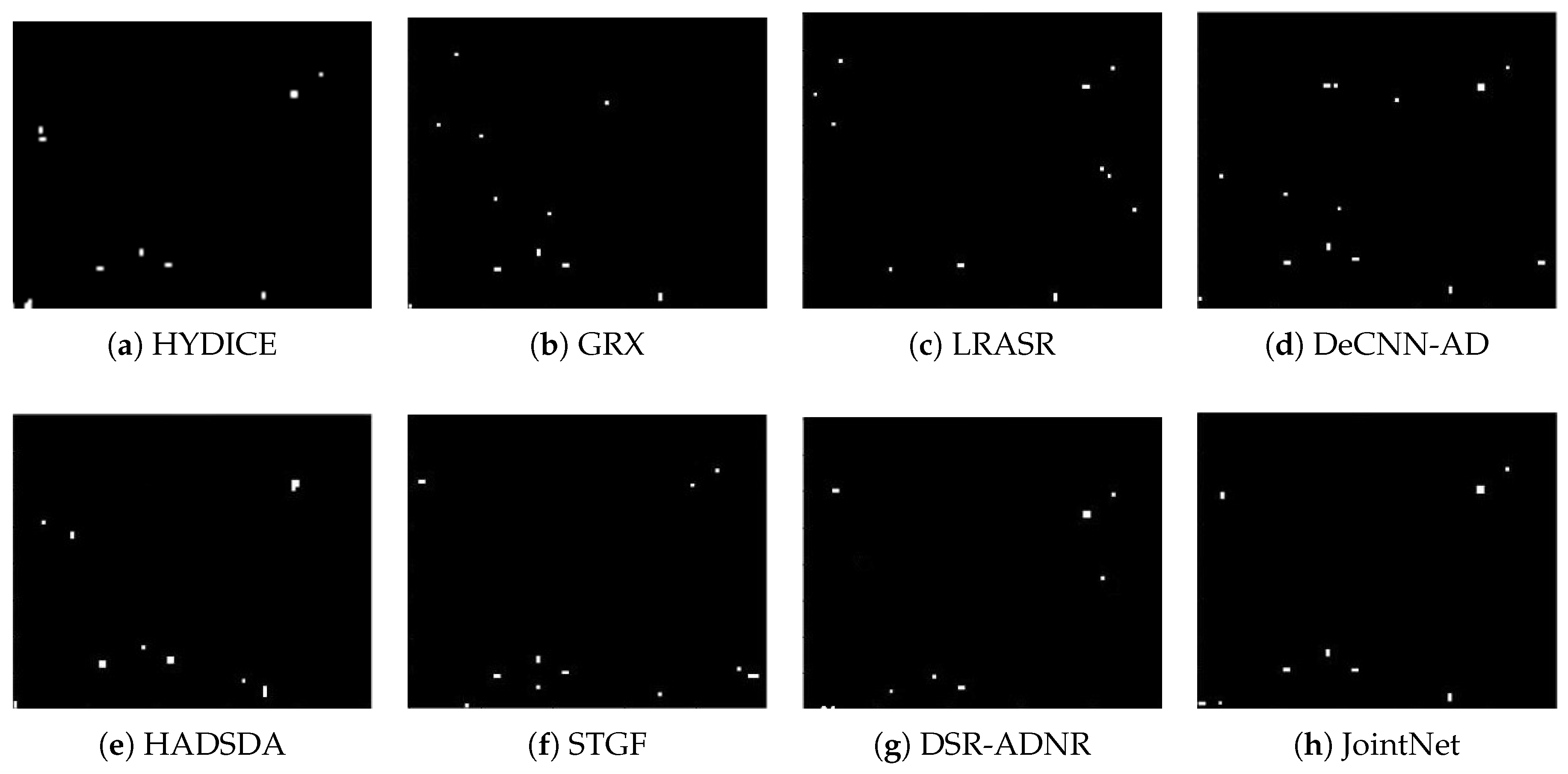
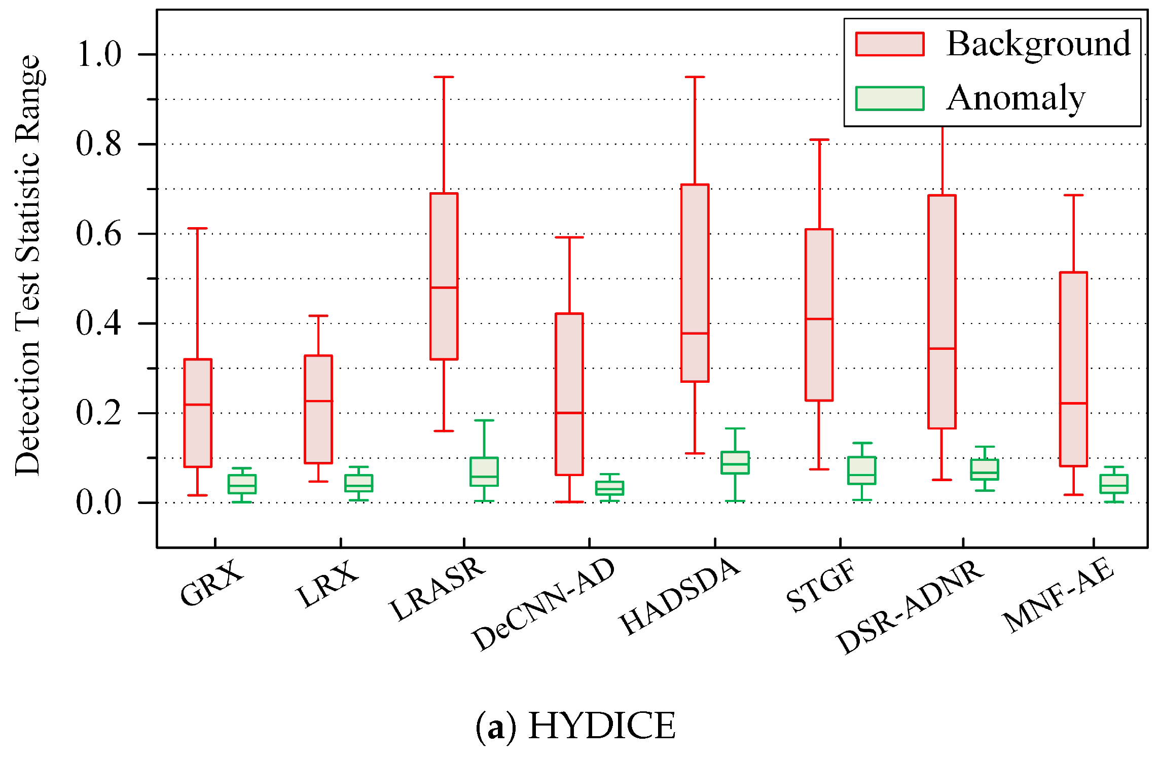
This section first analyzes the data structure of noisy HSIs, forming the basis for designing an MTL-based anomaly detection method. This approach allows the sharing of noise components from the denoising task with the anomaly detection task, providing richer and more comprehensive training data for both subtasks. Next, the JointNet model used in the proposed method is introduced, which fully exploits the deep information in the original image by integrating the denoising algorithm MNF with an AE. Following that, the concept of a noise score is introduced to evaluate the degree of abnormality for the pixel under test by using the shared noise information as a weighting factor, instead of relying on manually setting the thresholds, to improve the detection accuracy. Finally, appropriate local loss functions are designed for each subtask, which are combined into a total loss function to train the entire JointNet model, ensuring shared information flows throughout the network, thereby improving information utilization and completeness. 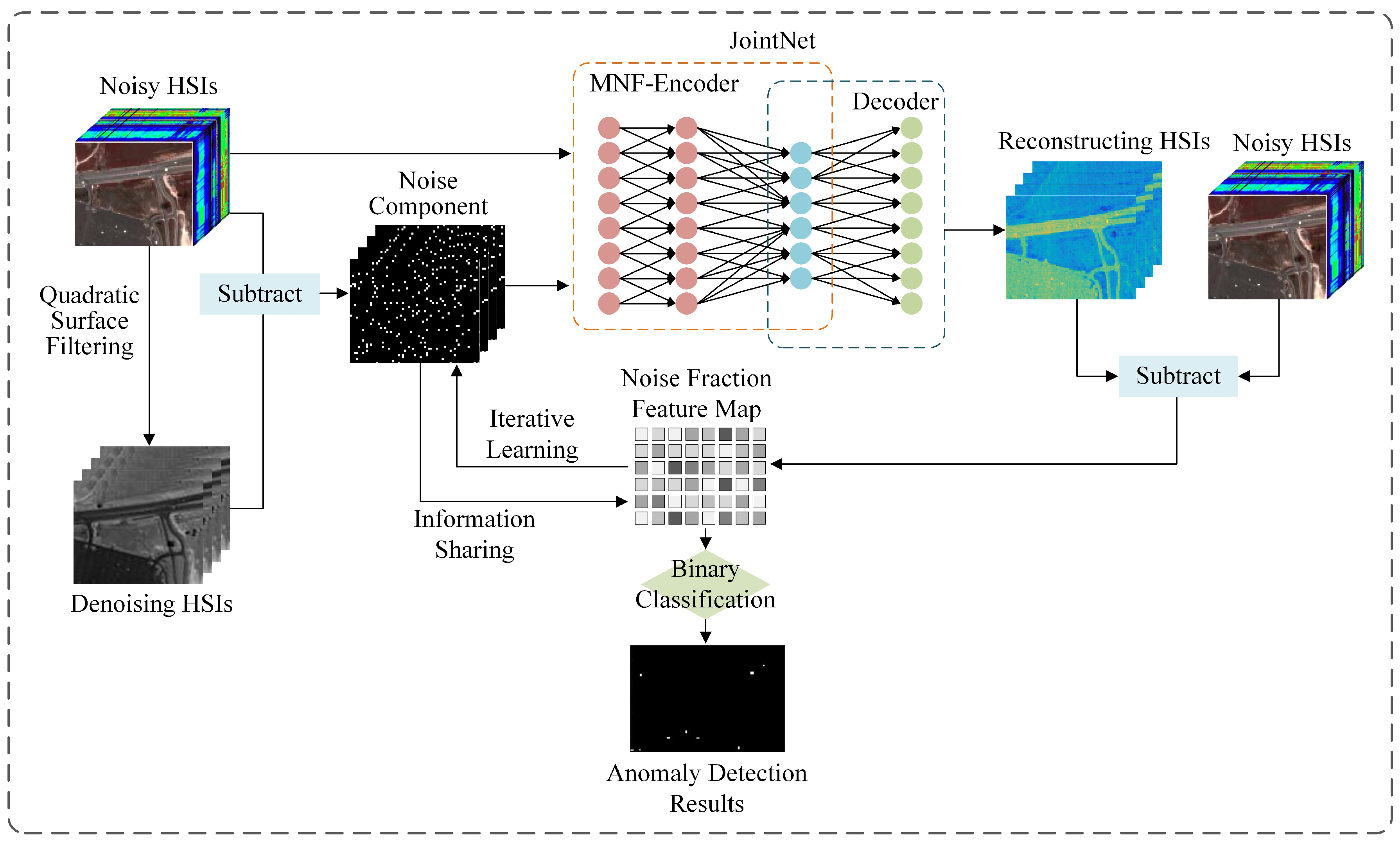Figure 2 shows the workflow of the methodology in this study.

3.1. Multitask-Learning-Based Noise Information Sharing

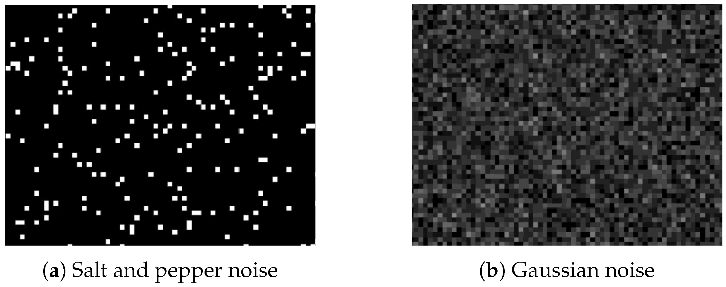
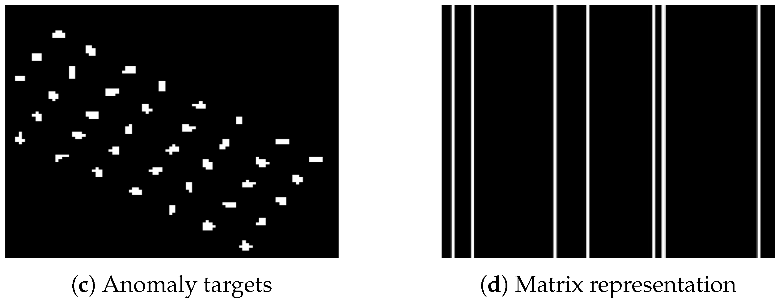
Our proposed method focuses on discrete noise. Each pixel in the HSI uniquely belongs to either the background or anomaly target category, while some pixels may simultaneously be considered noise, since noisy HSIs can contain overlapping noise and anomaly target pixels. This study modeled hyperspectral pixels using Equations (1) and (2). According to this model, the key to denoising a noisy HSI is to separate the pure anomaly target A from the HSI Y.

$$Y_i=B_i+N_i\left\{\begin{array}{cc}{N}_i=0\hfill & \mathrm{pure}\mathrm{background}\hfill \\ N_i\ne 0\hfill & \mathrm{noisy}\mathrm{background}\hfill \end{array}\right.$$

(1)

$$Y_i=A_i+N_i\left\{\begin{array}{cc}{N}_i=0\hfill & \mathrm{pure}\mathrm{anomaly}\mathrm{target}\hfill \\ N_i\ne 0\hfill & \mathrm{noisy}\mathrm{anomaly}\mathrm{target}\hfill \end{array}\right.$$

(2)

Efforts to improve the accuracy of noisy HSI anomaly detection have yielded significant results; yet, the impact of the noise introduced during data acquisition and transmission has not been adequately addressed. The typical processing flow for noisy HSI anomaly detection involves single-task learning, where denoising is followed by anomaly detection as two separate tasks. This approach has limitations in scenarios where anomaly targets are small, sparsely distributed, and similar to noise pixels, leading to misidentification during denoising and resulting in the loss of valuable data for anomaly detection. Since denoising and anomaly detection both use the same data source to learn hyperspectral features, there is a natural correlation between these tasks, suggesting that sharing feature information could lead to better results [37,38].

The proposed MTL-based method combines denoising and anomaly detection, allowing the shared noise information to improve the model’s learning capacity and detection accuracy. In the first subtask, the JointNet model is used to encode and decode the noisy HSIs, allowing the model to learn the inherent features of the noise, anomaly targets, and the background, while simultaneously denoising the image. By computing the difference between the original and reconstructed image, reconstruction errors can be derived. Due to the relatively low frequency of noise and anomaly targets, they tend to be suppressed during model training, leading to incomplete representation in the reconstructed image, resulting in a high reconstruction error, referred to as the “noise–anomaly target mixing component”. The second subtask involves designing a binary classification algorithm to extract pure anomaly target pixels from this mixing component and integrate them into the final anomaly detection results. Figure 2 shows the workflow of the MTL-based anomaly detection method for noisy HSIs. First, quadratic surface filtering is used to obtain a denoised HSI. The differential computation between the original noisy HSI and the denoised image provides the noise component, which serves as input to the JointNet model and as the weighting matrix for the noise score calculation. The original noisy HSI and noise component are then fed into the JointNet model, where the encoder comprising the noise-whitening and feature mapping modules produces the hidden layer coding. The decoder reconstructs the HSI from this coding. The difference between the reconstructed and the original noisy HSI yields the noise–anomaly target mixing component, using the noise scores’ calculation formula and a binary classification to obtain the final anomaly detection result.

3.2. JointNet Model

For noisy HSIs, some anomaly target pixels can morphologically resemble noise pixels [39,40], making them likely to be misinterpreted as noise and removed, leading to the failed detection of anomaly targets [41]. Since discrete noise has highly similar morphological and distributional characteristics to the anomaly targets, the spectral characteristics of the pixel are destroyed, and the attributes of the pixel to be tested cannot be determined, resulting in the loss of a judgment basis for the detection of anomalies. If we map the image to a new feature space to analyze the real spectral information of the noisy HSI and reconstruct the original hyperspectral signal that is not contaminated by noise, we realize the separation of noise and anomalous targets. Therefore, a method was developed to map the latent information in the original HSI, which contains both background and anomaly targets, to a new feature space using an autoencoder. This approach aims to filter out noise while retaining complete anomaly targets, avoiding missed detections. The AE comprises two parts: The encoder extracts hidden layer codes preserve the intrinsic features of the HSI, which plays a specific role in denoising, allowing the pure background to be used to construct a background dictionary. The decoder reconstructs the HSI based on the background dictionary and calculates the loss function during backpropagation to guide the encoder to select the most informative features. A noisy HSI has high data dimensionality, and using zero or random initialization of convolutional kernels in traditional deep neural networks may increase the computational cost. Given that one of the AE’s functions is denoising, applying the transformation matrix to the original HSI is equivalent to a linear transformation of the data. This paper proposes the JointNet model, which combines neural networks with the traditional denoising algorithm MNF based on principal component analysis (PCA) to obtain a set of convolutional kernel initial values for targeted learning, achieving the compression, denoising, and anomaly detection of noisy HSIs while minimizing the model training computational costs. The network architecture is composed of an encoder and a decoder.

(1)

Encoder: The encoder contains 12 convolution layers, and each layer consists of 3 × 3 convolutional operators, followed by batch normalization and a LeakyReLU activation function, and the outputs of the odd-numbered layers are simultaneously concatenated with the feature maps of the next odd-numbered layer through skip connections (except for layer #11). The first six layers implement the noise whitening, and the last six layers implement the feature mapping.

(2)

Decoder: The decoder contains 10 convolution layers consisting of 3 × 3 convolutional operators, which perform upsampling using nearest-neighbor interpolation.

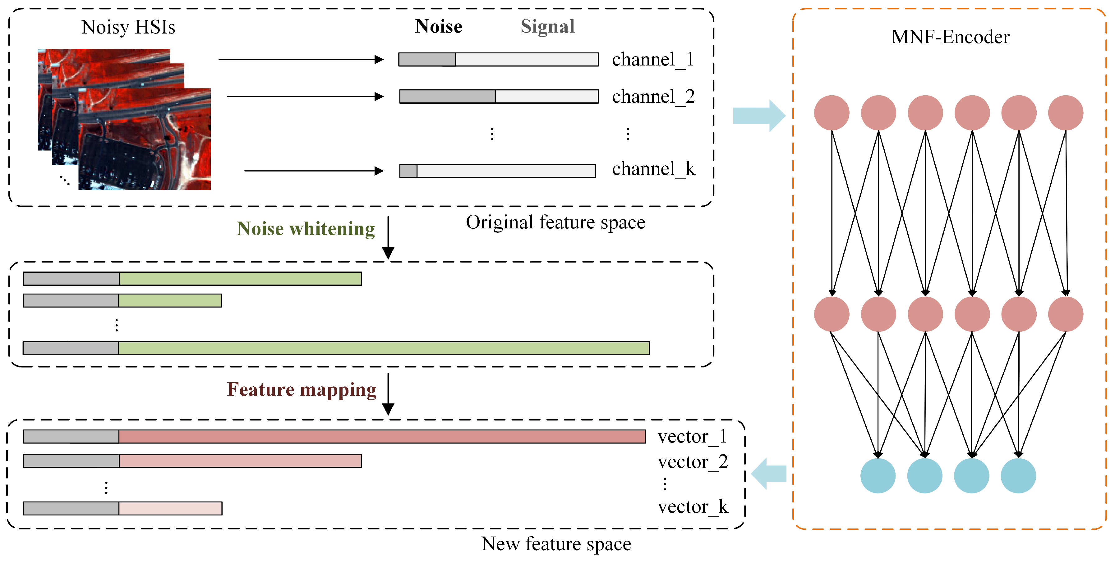
Figure 3 shows a schematic diagram of the MNF computation flow of the encoder. Through two steps, noise whitening and feature mapping, a total of three states exist in this computational flow for the noisy HSI. The first state occurs in the original feature space, where each rectangular bar represents the spectral vector of a pixel, consisting of a noise component and a signal component. In the second state, each rectangular bar represents a stretching of the spectral vector, where the corresponding signal-to-noise ratio of each vector is unchanged, but the noise component is a fixed value. The third state occurs in the new feature space, determining the direction of the basis vectors of the space, based on the magnitude of the signal component in the vectors, and the MNF rotation is accomplished. The JointNet model consists of two main modules: a noise-whitening module and a feature mapping module.

(1)

Noise-Whitening Phase

The key problem the MNF addresses is that calculating the signal-to-noise ratio for each spectral channel is challenging. The noise-whitening phase aims to convert the noise components in the HSI to a standard Gaussian distribution with a mean of 0 and a variance of 1, ensuring a fixed variance across all spectral channels. Assuming the HSI is a three-dimensional cube Y with dimensions $M\times N\times B$, a quadratic surface filter is used to generate the noise components N of the same size during the initial stage. A sliding window of size $k_1\times k_2\times b$ samples the noise components, reshaping them into column vectors with a mean normalization, denoted as $\widehat{N}$. The first $v_1$ eigenvectors of the $\widehat{N}$ matrix are selected and reshaped into a convolution kernel of size $v_1\times k_1\times k_2\times b$. This kernel is then used to convolve the HSI, producing the noise-whitened HSI.

(2)

Feature Mapping Phase

The feature mapping phase is similar to the noise-whitening stage, with the difference being that the sampled data come from the noise-whitened HSI, where the noise component’s variance is fixed. Principal component analysis is applied to the covariance matrix of the noise-whitened HSI. The top $v_2$ eigenvectors are selected based on descending eigenvalues, forming a convolution kernel of size $v_2\times k1\times k2\times b$. This kernel is used to convolve the noise-whitened HSI, mapping it to a new feature space, thereby achieving both denoising and spectral dimensionality reduction. Since the JointNet model calculates the signal-to-noise ratio of each spectral channel, the sliding window during sampling should cover as many spectral channels as possible, with convolution calculated across the corresponding receptive field.

Since the MNF’s core idea is principal component analysis, an important step is computing the transformation matrix, which defines the relationship between the original high-dimensional space and the new low-dimensional space. Applying the transformation matrix to the HSI is equivalent to taking the inner product of the matrix vectors with data vectors, a process similar to convolution. Since initializing convolution kernels for images can align with image features, it can accelerate network convergence. Thus, the MNF is used to derive initial convolution kernel parameters, replacing traditional zero or random initialization.

In summary, the primary process of denoising and reconstructing noisy HSIs using the JointNet model is as follows:

(1)

Noisy HSI Data Sampling

An HSI can be considered a three-dimensional (3D) cube with two spatial dimensions and one spectral dimension. In a 3D coordinate system, the x and y axes represent the spatial dimensions, and the b axis represents the spectral dimension. Since the convolution kernels need to cover the entire spectral range during dimensionality reduction, they must learn weights for different band regions. Selecting different spatial locations within the data cube is equivalent to sampling along the spectral dimension. Consider a cube of size $s\times s\times b_s$ for data sampling, targeting a fixed spectral range from $b_1$ to $b_2$ with a length of $b_s$. Sampling can be along the x axis or the y axis. This sampling process is repeated for various spectral ranges, and all the sampled data from the two moving directions are merged.

(2)

Convolutional Kernel Initialization

For each group of sampled data from different spectral ranges, principal component analysis is utilized to compute the first $v_1$ eigenvectors of the covariance matrix and reshape them into convolutional kernels, forming the first set of kernels. Using these kernels, convolution is performed on the original noisy HSI to produce the noise-whitened image. The kernel initialization step is repeated, replacing the sampled data with the noise-whitened HSI, and the first $v_2$ eigenvectors are selected to create the second set of convolution kernels. The method of initialization allows the convolutional kernel parameters to be targeted based on different spectral ranges, unlike zero or random initialization, providing a more suitable approach for HSIs compared to typical RGB images.

(3)

Convolution Calculation

Using the two sets of initialized convolution kernels, we apply them to different HSI data sources. The first set of kernels serves as a noise-whitening transformation matrix, altering the distribution of the noise component to conform to a standard Gaussian distribution with mean value of 0 and a variance of 1. Thus, these kernels should be applied to the original noisy HSI. The convolution result yields a noise-whitened HSI where the noise components between spectral channels have a consistent variance of 1. The second set of kernels acts as a feature-mapping transformation matrix, mapping the noise-whitened HSI to a low-dimensional feature space to explore new feature representations. This low-dimensional feature space is designed such that the noise components contribute minimally when mapped to the first basis vector and increase in significance with additional basis vectors. Given that each spectral channel’s noise component has a variance of 1, the noise level depends solely on the signal, i.e., the value of the noise-whitened image. Thus, the second set of convolution kernels should be applied to the noise-whitened HSI obtained from the first step of convolution calculation. At this stage, setting a stride greater than 1 allows for dimensionality resulting in a lower-dimensional HSI.

3.3. Noise Scores

In the current AE-based methods for HSI anomaly detection, the manual or automatic learning of thresholds is required to classify pixels as anomaly target or background pixels based on the reconstruction error. If the reconstruction error of the pixel to be tested is greater than the threshold, it is labeled as an anomaly target pixel. Otherwise, it is labeled as a background pixel. However, in noisy HSIs, anomaly target pixels may overlap with noise pixels, making it difficult to classify pixels accurately and reducing the detection precision and accuracy. Anomaly target pixels in noisy HSIs are usually clustered in small connected regions, whereas noise pixels are discretely and sparsely distributed. In addition, the noise component of noise pixels is always more significant than that of the anomaly target. Based on the above two data characteristics, for the MTL-based anomaly detection method, we proposesa noise score evaluation index using Equation (3) to evaluate the degree to which the pixel belongs, reducing the possibility of the missed detection of anomaly targets.

$$S_c=X_c{\displaystyle \frac{w_c}{{\sum }_{i=1}^9{w}_i}}-{\displaystyle \frac{1}{8}}\sum _{j=1}^8{X}_j{\displaystyle \frac{w_j}{{\sum }_{i=1}^9{w}_i}}$$

(3)

Here, S denotes the noise score, the subscript c represents the center pixel of the sliding window, $X_k$ represents the reconstruction error at spatial location k, $w_k$ indicates the activation value of the noise component at the spatial location k, ${\sum }_{i=1}^9$ encompasses all pixels within the sliding window, and ${\sum }_{j=1}^8$ represents the eight pixels surrounding the center pixel in the sliding window.

According to this method of calculating the noise score, if the center pixel of the sliding window is a noise pixel, its reconstruction error and noise component activation value differ significantly from the mean values of the neighboring pixels, making it impossible to represent them jointly and linearly. Consequently, the corresponding noise score is higher. Conversely, if the center pixel is an anomaly target pixel, its reconstruction error has only a minor difference from the mean value of the neighboring pixels, making it easier to represent them jointly and linearly. As a result, the corresponding noise score is lower. Following this principle, the spectral difference between the pixel under test and its neighboring pixels is computed using a representation learning approach, which serves as the basis for evaluating the extent to which the pixel belongs to the anomaly target. The noise score is computed pixel by pixel and then binary-classified to obtain the initial set of anomaly target pixels. This set is then refined by merging neighboring pixels and removing discrete ones to yield the final abnormal target detection result.

3.4. Loss Function

Reasonable local loss functions were designed for Subtask I and Subtask II and combined to form the total loss function, enabling MTL to denoise HSIS and detect the anomalies in HSIs.

For Subtask I, the computational principle of the MNF algorithm is integrated with a deep neural network AE. This combination compresses the spectral channel information from the noisy HSI, which has a low signal-to-noise ratio and poor image quality, into a new low-dimensional feature space layer by layer. This process retains valuable signals representing both anomaly targets and the background portions of the original image. Firstly, the AE aims to analyze the properties of the pixels to be tested using the reconstruction error between the original and reconstructed images. Therefore, a regularization term Equation (4) was designed to quantify the reconstruction error, serving as the first part of the local loss function for Subtask I.

$$L_{res}=\left|\right|X-\widehat{X}\left|\right|$$

(4)

Here, $L_{res}$ represents the differential computation loss function, X represents the noisy HSI, and $\widehat{X}$ is the reconstructed image output by the JointNet model. The difference between these images reflects the magnitude of the reconstruction error.

Next, considering the sparse and discrete distribution of noise in noisy HSIs, the $L_{2,1}$ norm is utilized as the second part of the local loss function for Subtask I. The computation is shown in Equation (5).

$$L_{2,1}=\sum _{i=1}^m\sqrt{\sum _{j=1}^n{w}_{ij}^2}$$

(5)

Here, $W=relu\left(N\right)$ represents the activation matrix of the noise component, N represents the noise component, m indicates the number of feature groups, and n represents the number of features within each group. The $L_{2,1}$ paradigm is also known as group sparse regularization, where ${\sum }_{j=1}^n{w}_{ij}^2$ computes the $L_2$ paradigm of all the features in the ith group, and ${\sum }_{i=1}^m$ denotes the $L_1$ paradigm regularization of the $L_2$ paradigm of all the groups, which combines the characteristics of the $L_1$ paradigm and the $L_2$ paradigm. For handling multistructured features, it achieves intergroup sparsity while maintaining intragroup feature density, aligning with the property of using noise components to restrict the distribution of anomaly targets.

In summary, the local loss function for Subtask I is given by Equation (6).

$$L_{res}+L_{2,1}=\left|\right|X-\widehat{X}\left|\right|+{\left|\right|W\left|\right|}_{2,1}$$

(6)

For Subtask II, the reconstruction error is obtained by subtracting the reconstructed image output by the JointNet from the noisy HSI. Pixels with significant reconstruction errors form the noise–anomaly target mixing component. Filtering anomaly targets from this mixing component is treated as a binary classification problem. Hence, the cross-entropy loss function Equation (7) is adopted as the optimization objective for Subtask II.

$$L_{CE}=-\sum _{i=1}^{mn}p\left(X_i\right)log\left(q\left(X_i\right)\right)$$

(7)

Here, $L_{CE}$ represents the loss function of Subtask II, ∑ represents the summation function, $p\left(X_i\right)$ represents the label of the pixel to be tested, which is numerically equivalent to the activation value of the noise component in Subtask I, and $q\left(X_i\right)$ is the predicted probability that the pixel belongs to the noise, which is equivalent to the noise scores. This local loss function realizes the application of MTL ideas by sharing the noise component between the denoising and anomaly detection.

In summary, the total loss function of the proposed method consists of the local loss functions for Subtasks I and II, as shown in Equation (8).

$$\begin{array}{cc}\hfill L=& L_{res}+\alpha L_{2,1}+\beta L_{CE}=\left|\right|X-\widehat{X}{\left|\right|}_2+{\alpha \left|\right|W\left|\right|}_{2,1}\hfill \\ \hfill -& \beta \sum _{i=1}^{MN}p\left(X_i\right){log}_{(}q\left(X_i\right))\hfill \end{array}$$

(8)

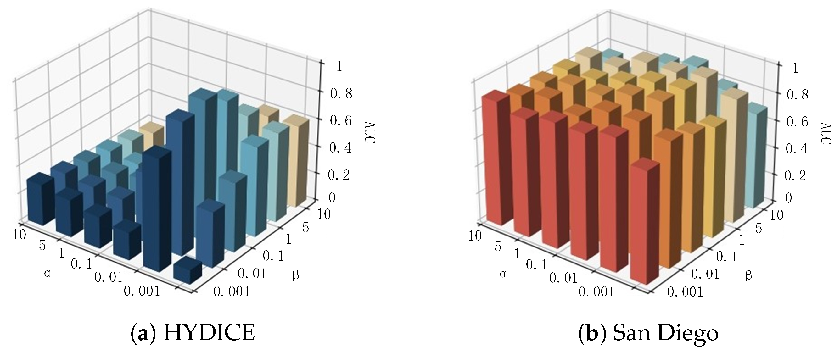
Here, L represents the total loss function, serving as the final optimization objective of noisy HSI anomaly detection based on MTL, and $\alpha$ and $\beta$ are regularization parameters. This loss function enables the achievement of three objectives: (1) analyzing noise distribution characteristics and morphological features, denoising the noisy HSI, and utilizing the noise component as prior information for anomaly detection, enriching the information available for both subtasks; (2) generating a denoised HSI without noise and accurately representing the background portion; and (3) considering the influence of noise and intrinsic data characteristics to calculate the anomaly degree of the pixel, thereby avoiding misclassifying anomaly target pixels as noise pixels.

4. Experiments

In this section, the extensive experiments conducted to evaluate the performance of the proposed model and method are described. The first subsection introduces the two datasets used for the experiments. The second subsection describes the experimental verification of the impact of the relevant parameters on the detection accuracy of the JointNet model. The third subsection analyzes the noise robustness of the JointNet model. The fourth subsection describes the verification of the effectiveness of the noise-whitening module, feature mapping module, MTL information-sharing module, and noise score module through ablation experiments. Finally, several existing denoising HSIs and anomaly detection algorithms are compared, demonstrating the good detection capabilities of the proposed JointNet model and method in terms of the experimental results and the visualization effects. Each experiment was conducted using Pycharm on a computer equipped with an Intel(R) Core(TM) i7-13700KF 3.40 GHz CPU and an NVIDIA GeForce RTX 4070 Ti GPU.

4.1. Experimental Datasets

(1)

HYDICE Datasets: This dataset, widely used in remote sensing and earth science research, was captured by the Hyperspectral Digital Image Collection Experiment Airborne Sensor (HYDICE) aboard the ER-2 High-Altitude Vehicle (HAV) aircraft, flying at high altitudes to photograph the ground over urban areas in California. Subimages with a size of 80 × 100 pixels were selected for the experiment, excluding bands with high water vapor absorption and damage, to obtain 175 bands for the anomaly detection experiments. The wavelengths ranged from 400 to 2500 nm, covering the visible and infrared spectral ranges. The spatial resolution was 3 m/pixel. The background components included vegetation, highways, and parking lots, while 21 pixels representing artificial vehicles were considered anomaly targets.

(2)

San Diego Dataset: This dataset was collected by the AVIRIS sensor in the San Diego Airport area in California, USA. This dataset has an image size of $100\times 100$, the spatial resolution was 3.5 m, and a spectral resolution of 10 nm, covering wavelengths from 370 to 2510 nm. After excluding 35 absorption bands and channels heavily affected by the atmosphere, experiments were conducted on 189 spectral bands. The background components included airplane hangars, aprons, and soil, while three airplanes with 58 pixels were considered anomaly target pixels.

4.2. Parameter Settings

The proposed MTL-based anomaly detection method for noisy HSI in this work involves two sets of essential parameters. The first group comprises the two regularization parameters $\alpha$ and $\beta$ in the total loss function, while the second group includes the number of convolution kernels in the noise-whitening and feature mapping module.

(1)

Regularization parameter for the loss function

For the loss function used in the proposed MTL-based anomaly detection method for noisy HSI, which includes two regularization parameters $\alpha$ and $\beta$, experiments were designed to verify their effects on the anomaly detection results measured using the $AUC$. Specifically, $\alpha$ and $\beta$ control the weights of the local loss function corresponding to the denoising and anomaly detection subtasks, respectively; they were set to 0.001, 0.01, 0.1, 1, 5, and 10, and the loss functions with different parameter combinations were used for learning and updating the parameters of the JointNet model. Figure 4 shows the effect of the loss function regularization parameters $\alpha$ and $\beta$ on the AUC. After experimental validation, $\alpha =0.01$ and $\beta =0.1$ yielded the maximum $AUC$, indicating the better training and detection effects of the model using this parameter setting. Therefore, the regularization parameters for the loss function in the subsequent experiments were set to $\alpha =0.01$ and $\beta =0.1$.

(2)

Number of convolutional kernels for JointNet models

Another important set of parameters in the JointNet model used in the proposed MTL-based anomaly detection method for noisy HSIs is the number of convolution kernels in the noise-whitening and feature mapping module, essentially corresponding to the number of eigenvectors in the two principal component analyses, $v_1$ and $v_2$. To ensure balance in the image compression between the two modules, assuming $v_1=v_2$, experiments were designed to verify the effect of these parameters on the reconstruction of the HSI using the JointNet model. From the experimental results shown in

Table 1. Influence of the number of convolutional kernels $v_1$ and $v_2$ on the image reconstruction.

${\mathit{v}}_1/{\mathit{v}}_2$	PSNR	SSIM	SAM	Time(s)
1	41.24	0.89	4.37	136.49
2	42.71	0.91	4.12	138.50
3	42.36	0.87	4.91	139.35

, when the number of convolution kernels was 2, $v_1=v_2=2$, the image deviation between the spectral channels was minimal, and the JointNet model exhibited the best reconstruction effect on the original HSI. Therefore, the number of convolution kernels for both the noise-whitening and the feature mapping modules of the JointNet model in the subsequent experiments was set to $v_1=v_2=2$.

4.3. Noise Robustness Analysis

The method proposed in this paper targets discrete noises similar in morphology and distribution to the anomaly target, typically including salt and pepper noise and Gaussian noise. To verify the JointNet model’s robustness against noise, experiments were designed to evaluate its denoising performance on different types of noise. The specific steps were as follows: first, two types of simulated noise were added to the HSI; then the encoder and decoder of JointNet model was used to reconstruct the images; finally, the four sets of reconstructed images were compared and evaluated with the original HSI using quantitative denoising evaluation metrics to confirm the JointNet model’s robustness regarding noise type and distribution. The simulated noises were categorized as follows:

• ${\sigma }_n$ = rand (10): randomly selecting 10% of all pixels and adding salt and pepper noise, setting these pixel values to 0;
• ${\sigma }_n$ = rand (20): randomly selecting 20% of all pixels and adding salt and pepper noise, setting these pixel values to 0;
• ${\sigma }_n$ = Gau (0,0.01): randomly adding Gaussian noise with a mean of 0 and variance of 0.01 to all pixels;
• ${\sigma }_n$ = Gau (0,0.02): randomly adding Gaussian noise with a mean of 0 and variance of 0.02 to all pixels.

The experimental results, shown in

Table 2. Table of experimental results on the robustness of the JointNet model to various noise types.

Noise	PSNR	SSIM	SAM
${\sigma }_n$ = rand (10)	39.845	0.623	4.439
${\sigma }_n$ = rand (20)	37.486	0.678	4.592
${\sigma }_n$ = Gau (0,0.01)	43.516	0.913	3.697
${\sigma }_n$ = Gau (0,0.02)	41.967	0.843	3.796

and Figure 5, indicate that compared to the reference simulated noise, Gaussian noise with a mean value of 0 and variance of 0.01 exhibited a higher PSNR and an SSIM, and a lower SAM, suggesting the JointNet model effectively modeled and eliminated this type of noise. Consequently, subsequent experiments utilized Gaussian noise distributed as $G(0,0.01)$ for denoising validation.

4.4. Ablation Study

4.4.1. Performance Analysis of JointNet

To assess the JointNet model’s reconstruction effect on noisy HSIs, experiments with two task modes were conducted as follows:

Case 1: Single task. First, we denoised the noisy HSI using minimal noise fraction transformation. Then, we reconstructed the denoised image using a simple AE model, and, finally, we compared and computed the image quality evaluation metrics against the noisy HSI.

Case 2: Multiple tasks. Simultaneously, we input simulated Gaussian noise and the noisy HSI into the JointNet model, generating a noise-free reconstructed HSI. Then, we compared it with the noisy HSI and calculated the image quality evaluation metrics.

Table 3. Effectiveness of the JointNet model in the reconstruction of noisy hyperspectral images.

	MSE	PSNR	SSIM	SAM	Time(s)
Case 1	$8.93\times {10}^{-7}$	38.271	0.902	3.949	128.674
Case 2	$6.94\times {10}^{-4}$	43.971	0.913	3.763	159.321

presents the results of these experiments.

As shown in Table 3, for the experiments in single-task mode, the MSE was lower than that of the multitask mode. For the experiments in the multitask mode, the PSNR and SSIM were higher, and the SAM was lower. This indicates the JointNet model’s superior reconstruction compared to the separate applications of the MNF and AE, highlighting the effectiveness of integrating the denoising and reconstruction processes. The anomaly detector received full HSI detail and thus was more sensitive to small differences in spectral features. Targeted denoising methods designed to suit HSI characteristics can enhance information integrity in feature extraction, obtaining better detection accuracy.

Visualizing the feature map output from the JointNet model’s feature mapping module, the denoised images were obtained through up-sampling convolutional computation, verifying whether the MNF algorithms contributed to denoising during training. The denoised HSIs were then compared with outputs from traditional and deep learning denoising algorithms, as shown in Figure 6.

Figure 6 reveals that the denoised images output by the encoder of JointNet contained minimal noise and retained the most detailed parts compared to other common denoising algorithms, in particular, the anomaly targets. It shows that the deep neural network structure of the AE is suitable for high-dimensional HSI data, and the combination with the MNF algorithm based on the principle of signal energy can avoid the anomaly targets being corrupted due to the morphological similarity, showing its superior denoising capability.

4.4.2. Effectiveness of Multitask Learning

To evaluate the MTL’s enhancement of the denoising and anomaly detection, ablation experiments on the loss function were conducted. Comparing the single-task and MTL scenarios using the JointNet model for anomaly detection on noisy HSIs, the accuracy and runtime were measured. In Loss I, the loss function for single-task learning solely comprised the difference computation $L_{res}$. In this scenario, there was no transfer of noise components from the denoising subtask to the anomaly detection subtask. During the detection stage, the determination of whether a pixel belonged to anomaly targets relied solely on the reconstruction error of that pixel. In Loss IV, the loss function for MTL incorporated the local loss functions corresponding to the denoising and anomaly detection subtasks, expressed as $L_{res}+L_{2,1}+L_{CE}$. In this context, noise components were transferred from the denoising subtask to the anomaly detection subtask as prior information for prediction of the label of the pixel being tested, and the detection stage completed the label determination through calculation of the noise scores of all the pixels and binary classification. Building upon Loss I, for Loss II and III, we introduced regularization terms $L_{2,1}$ forthe noise fraction and $L_{CE}$ for the predicted labels, respectively, to assess the effectiveness of the MTL. The experimental results are presented in

Table 4. Multitask learning loss function ablation experiment.

Loss	Time (s)	AUC
Loss I	260.384	0.873
Loss II	348.382	0.883
Loss III	361.359	0.902
Loss IV	366.325	0.916

.

As shown in Table 4, the AUC for Loss IV was the maximum in this group of experiments, indicating that updating the parameters of JointNet using the total loss function was the most effective for anomaly detection, validating the effectiveness of the MTL. In addition, the AUC values for Loss II and III were higher than that of Loss I, suggesting that combining two subtasks and sharing information for anomaly detection yielded greater improvement than single-task learning. This also demonstrates that the MTL has a positive effect on improving the accuracy and precision of anomaly detection from noisy HSIs.

4.5. Comparison Experiments

4.5.1. Denoising

To verify the computational performance of the proposed denoising methods, this section describes the comparison of JointNet with traditional and deep learning denoising and anomaly detection methods. The denoising methods include traditional PCA, wavelet transform, Fourier transform, and deep learning BM3D [42] and DeCNN-AD [34] algorithms.

Table 5. Comparison results of denoising algorithms on the hyperspectral image datasets.

		PSNR	SSIM	SAM	AUC
HYDICE	PCA	31.36	0.79	8.930	0.796
	Wavelet transform	35.90	0.75	7.926	0.782
	Fourier transform	42.14	0.86	6.774	0.849
	BM3D	39.41	0.83	12.717	0.896
	DeCNN-AD	39.67	0.89	6.499	0.903
	JointNet	41.79	0.91	4.350	0.916
San Diego	PCA	26.72	0.67	3.876	0.886
	Wavelet transform	31.37	0.74	4.791	0.916
	Fourier transform	36.75	0.84	5.779	0.812
	BM3D	34.53	0.82	6.003	0.850
	DeCNN-AD	41.74	0.87	9.646	0.901
	JointNet	42.83	0.93	3.558	0.920

presents the comparison results of the denoising algorithms on the HYDICE dataset and the San Diego dataset. As indicated in Table 5, observing the reconstructed images generated by the decoder of the JointNet and comparing the denoising algorithms, JointNet outperformed the other algorithms in terms of PSNR, SSIM, SAM, and AUC. This indicates the JointNet implements the mathematical concept of the MNF algorithm in denoising and utilizes the deep neural network’s capabilities to extract information from high-dimensional HSI. This enables the preservation of valuable signals and the removal of noise signals during gradual dimensionality reduction.

Figure 7 and Figure 8 depict the difference between the spectral curves denoised by each denoising algorithm and the corresponding pixels in the original noiseless image on the HYDICE and San Diego datasets. Both figures demonstrate that the JointNet proposed in this article exhibits the smallest difference from the spectral features of noiseless image elements, indicating superior denoising performance and excellent preservation of original spectral information with minimal destruction of image details, addressing the problem of existing denoising algorithms mistakenly removing anomaly targets as noise.

4.5.2. Anomaly Detection

To verify the computational performance of the proposed anomaly detection methods, this section compares JointNet with the traditional and deep learning anomaly detection methods, including traditional GRX, CRD, LRASR [43], and the deep learning DeCNN-AD, HADSDA [44], STGF [14], and DSR-ADNR [36] algorithms.

Table 6. Comparison results of the anomaly detection algorithms on the HYDICE dataset.

	GRX	CRD	LRASR	DeCNN-AD	HADSDA	STGF	DSR-ADNR	JointNet
AUC	0.901	0.925	0.915	0.920	0.939	0.863	0.932	0.943
Time (s)	0.26	60.34	74.90	54.73	33.58	35.20	29.40	162.39

presents a comparison of the results of the anomaly detection algorithms on the HYDICE dataset, and

Table 7. Comparison results of the anomaly detection algorithms on the San Diego dataset.

	GRX	CRD	LRASR	DeCNN-AD	HADSDA	STGF	DSR-ADNR	JointNet
AUC	0.870	0.887	0.923	0.892	0.914	0.948	0.906	0.959
Time (s)	0.45	65.10	85.61	70.09	48.50	25.83	16.91	126.57

shows a comparison of the results on the San Diego dataset. An analysis of these tables indicates that the proposed anomaly detection method, JointNe, achieves the highest AUC value among the compared algorithms, demonstrating superior anomaly detection performance.

Figure 9 and Figure 10 present the anomaly detection results on the HYDICE and San Diego datasets, respectively. The analysis of these figures reveals that certain anomaly target pixels were missed by the GRX, LRASR, and DSR-ADNR algorithms, while the DeCNN-AD, HADSDA, and STGF algorithms incorrectly identified noisy pixels or detailed textured pixels as anomaly targets. Notably, the anomaly detection results obtained by the JointNet method closely resembled the groundtruth maps. This is attributed to the MTL-based HSI anomaly detection method JointNet, which combines denoising and anomaly detection tasks, strengthening the anomaly detection by leveraging the shared noise information as prior reference information.

Figure 11 depicts box plots of the anomaly detection results for the comparison of the algorithms on the HYDICE and San Diogo datasets. In this figure, the red boxes represent the distribution of anomaly target pixels, while the green boxes represent the background pixels. The larger the vertical distance between the two box shapes, the more distant the two data distribution models, indicating the effectiveness of the anomaly detection algorithm. According to these plots, the anomaly target box shapes of the GRX and DeCNN-AD algorithms are too short, reflecting, to some extent, the likelihood of missed anomaly pixels. Conversely, the anomaly target box shapes of LRASR, HADSDA, STGF, and DSR-ADNR algorithms cover most of the hyperspectral data values. However, the overlap with the anomaly target box shape, due to the excessively long background box shapes of these three algorithms, indicates that some background pixels are incorrectly recognized as anomaly target pixels. The anomaly target and background box shapes of the JointNet method exhibit a reasonable distribution with minimal overlap, and the small size of the background box shapes aligns with the low rank of the background partial atom vectors in the HSI. In conclusion, it can be stated that the JointNet method provides the most effective anomaly detection.

5. Conclusions

This study developed a multitask-leawasrning-based anomaly detection method for noisy HSIs to enhance the accuracy of anomaly detection. Firstly, the JointNet model is designed to integrate the denoising algorithm MNF into an autoencoder model, addressing the issue of independent denoising tasks leading to the loss of image details, especially anomaly targets. Secondly, a new loss function was designed to facilitate the sharing of the noise information between the two subtasks of denoising HSIs and anomaly detection through joint learning, resolving the issue of the underutilization of inherent information. Finally, a noise score calculation method was develoepd to estimate the anomaly level of each pixel by considering the morphology and distribution characteristics, resolving the issue of overlapping noise and anomaly target pixels leading to inaccurate classification. The effectiveness of the proposed model and method was validated by testing on the HYDICE and San Diego datasets. The denoising metrics and the anomaly detection AUC in the two datasets were both higher than those of the algorithms used for comparison, indicating that the proposed model and method improve the distribution estimation and anomaly detection accuracy and reduce the information loss in the denoising stage of anomaly detection tasks. In future work, we will investigate more efficient methods for removing the mixed noise in HSI data, such as stripe noise and deadlines.

The above experimental results and analysis show that both the model and the method proposed in this article are effective for the task of anomaly detection with noisy images. In subsequent research, we will further refine the model, using more advanced variants such as variational autoencoder (VAE) and adversarial autoencoder (AAE), and try to collect real datasets for testing to verify the feasibility of the proposed model and method in complex scenarios.