1. Introduction
Ubiquitous radar, also known as holographic staring radar or floodlight radar [
1,
2], was defined by the IEEE Radar Definition Standard in 2017 as a radar system that looks everywhere all the time and performs multiple functions simultaneously rather than sequentially [
3]. Due to its full spatio-temporal coverage characteristic, there is no need for beam scanning or complex resource scheduling. This enables simultaneous detection and tracking of a large number of targets at high data rates. Additionally, it does not require beam scanning and enables longer integration times and higher Doppler resolution. The high Doppler resolution effectively separates moving targets from clutter and provides a new dimension for target feature extraction and identification [
4]. However, the use of a low-gain wide-beam transmitting antenna in this radar can result in weaker received target echoes. To address this problem, ubiquitous radar adopts the long-time coherent integration (LTCI) technique [
5], which enhances the detection capability. Nonetheless, the motion of high-speed and highly maneuverable targets introduce challenges such as Doppler frequency migration (DFM), range migration (RM), and velocity ambiguity (VA), which can degrade coherent integration performance.
Currently, a lot of research is underway to address target movement compensation in the LTCI process. However, coherent methods typically do not support multi-target scenarios and often involve substantial computational overhead, limiting their practical engineering applications. In contrast, hybrid integration methods offer significant advantages by effectively balancing performance and computational complexity.
In traditional target detection and tracking, the common approach involves using a constant false alarm rate (CFAR) for target detection, followed by filtering the detection results for tracking, a method also known as detect-before-track (DBT). However, in complex backgrounds with dense clutter and strong electromagnetic interference, CFAR processing often struggles to adequately control false alarms due to challenges in modeling clutter and interference. On the one hand, to increase target detection probability, CFAR processing tends to result in a high false alarm rate, leading to a significant number of false detections during track initiation, which in turn affects track association and tracking. On the other hand, attempting to reduce the false alarm rate by raising detection thresholds can result in missed detections of weak targets with low SNR [
6]. To address these issues, the track-before-detect (TBD) algorithm was proposed in the 1970s [
7].
The TBD method is capable of achieving incoherent integration, leveraging signal processing algorithms to detect targets even in the presence of significant noise interference. TBD establishes tracks for potential targets prior to official detection, enhancing radar system performance in scenarios with weak target signals or challenging clutter and interference environments [
8,
9]. Unlike the DBT approach, TBD does not apply threshold detection to individual frames but instead utilizes joint processing across multiple frames to exploit differences in target–background (e.g., noise or clutter) inter-frame positional correlations. This method effectively accumulates target echo energy and suppresses background clutter [
10]. Additionally, TBD ensures robust detection by utilizing data accumulated up to the current time step for tracking, rather than relying only on data from the current time step [
11].
There are multiple algorithms available for implementing TBD, which can generally be classified into two categories: batch algorithms and recursive algorithms. Examples of batch algorithms include the Hough transform (HT) and dynamic programming (DP), as demonstrated in studies such as [
12,
13,
14,
15,
16]. These methods involve storing and processing received data over a specified time period, requiring multiple scan times for accurate results. However, these algorithms do not exploit the correlation between different batches, requiring substantial data storage and exhibiting high computational complexity. And their poor real-time performance makes them unsuitable for tracking maneuvering targets [
17].
Recursive algorithms iteratively predict and update target state estimations, aligning well with the comprehensive coverage capabilities of ubiquitous radar across space and time. The particle filter (PF) is a common choice for TBD applications due to its effectiveness in handling non-Gaussian and nonlinear scenarios [
18,
19,
20]. PF-TBD, initially proposed by Salmond [
21,
22] introduces improvements over earlier methods. However, most TBD research is limited to single-target scenarios and cannot effectively handle complex situations with varying and unknown numbers of targets.
In scenarios with unknown and time-varying numbers of targets, finite set statistics offer a robust Bayesian inference framework for multi-target filtering, grounded in random finite set (RFS) theory [
23]. The probability hypothesis density (PHD) filter [
24], as a moment-based approximation solution for multi-target Bayesian filtering, has received sustained attention and is widely implemented using sequential Monte Carlo (SMC) methods due to its proven convergence properties [
25]. Compared to traditional methods, the PHD filter does not require data association, which typically leads to exponential computational complexity with increasing numbers of targets and observations. Hence, the PHD filter is recognized as a computationally efficient approach for multi-target tracking.
Most existing research on detecting high-speed and high-maneuvering targets is limited to single-target scenarios, which oversimplifies tracking challenges. However, the more typical scenario involves an unknown and varying number of targets within the surveillance area, often complicated by clutter that obscures sensor measurements. Furthermore, sensor measurements are typically subject to noise and inherent errors. The complexity is further compounded during high-speed and high-maneuvering target motions due to factors like RM, DFM, and VA. To tackle these issues, we propose a hybrid integration approach in this paper, leveraging LTCI, PHD, and TBD to effectively achieve joint detection and estimation of multiple weak, high-speed, and high-maneuvering targets. The proposed method is referred to as KT-MFP-ISMC-PHD-TBD, where the ‘MFP’ stands for matched filter processing, and the letter ‘I’ signifies ‘improved’.
In the KT-MFP method, the first-order RM is compensated using KT. Different folding factors are then applied to generate the corresponding sub-range-Doppler (SRD) planes for VA compensation, which are subsequently stitched together to form the extended range-Doppler (ERD) plane. In the TBD method, tracking is directly performed on the ERD plane. The PHD filter is used to propagate the multi-target states, and an amplitude-based adaptive prior distribution method along with the LSM observation model for DFM compensation is proposed. Furthermore, a particle space projection method is introduced. The SRD planes are stacked to form a folding range-Doppler (FRD) space, particles are projected along the folding factor dimension, and clustering is performed on the particles to eliminate the effects of mirror targets. Ultimately, simulation experiments demonstrate that the proposed method outperforms traditional methods, exhibiting superior performance and robustness, achieving a balance between performance and efficiency. Actual data from ubiquitous radar also verify the proposed method’s ability to detect and track multiple high-speed, highly maneuverable targets.
The structure of this paper is as follows.
Section 2 outlines the theoretical derivation of KT-MFP and the method for generating the ERD plane.
Section 3 describes the improved SMC-PHD filter and details the implementation of TBD.
Section 4 conducts comparative experiments and validates the proposed method using actual measurement data.
Section 5 provides the conclusions.
2. Keystone Transform and Matched Filter Processing
The radar transmission signal can be expressed as follows:
where
signifies the fast time,
(
) denotes the slow time,
refers to the pulse repetition interval (PRI), and
is the number of coherent integration pulses.
denotes the pulse width,
represents the frequency modulation rate,
stands for the carrier frequency.
After the transmitted signal undergoes backscattering from the target, and subsequent down-conversion and pulse compression by the radar receiver, the resulting signal in the frequency–slow-time domain is given by
where
is the amplitude,
is the coherent integration time,
B represents the bandwidth of transmission signal, and
c is the light speed.
stands for the instantaneous radial range of the target, which can be expressed as
where
is the pulse repetition frequency (PRF), and
signifies the wavelength.
,
,
, and
represent the radial range, baseband velocity, ambiguity number, and acceleration of the target, respectively.
Then, we substitute (
3) into (
2) and obtain
In [
26,
27,
28], the expression of KT is denoted as
where
denotes the new slow-time variable. From the equation above, it can be observed that as
f increases,
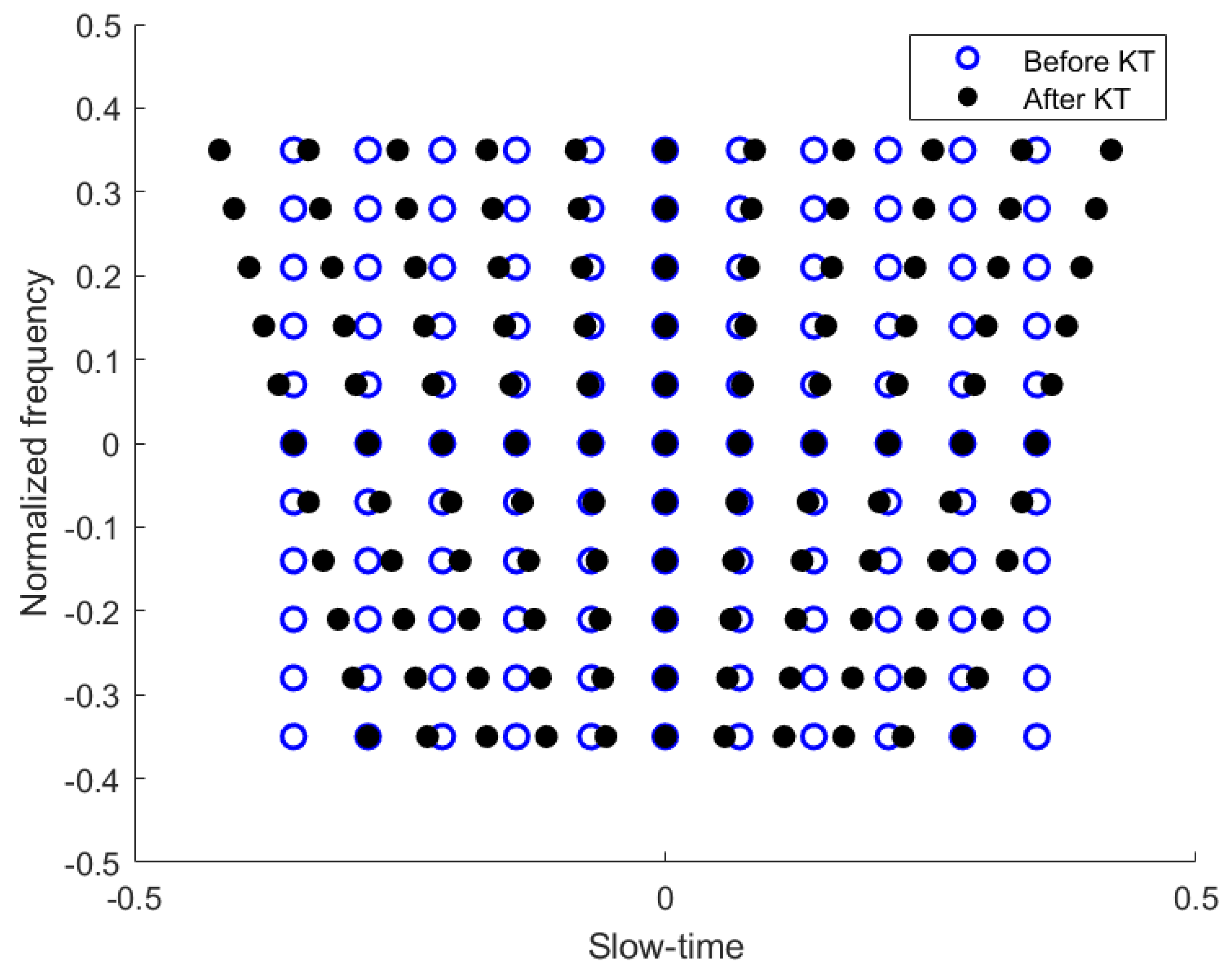
representing the sampling interval becomes larger. KT fundamentally constitutes a scale transformation on the slow time, altering the sampling interval of the slow-time sampling points. The points in the RD plane before and after KT are depicted in
Figure 1. The figure reveals that the sampling interval along the slow-time dimension is uniform before applying KT, whereas after KT, the slow-time sampling interval varies with
f.
Then, we substitute (
5) into (
4) to decouple
f and
. Because
, we can obtain
Equation (
6) indicates that due to the ambiguity velocity,
f and
are coupled, which will lead to the aggravation of RM. Therefore, we use the MFP technique to construct a matched filter as follows:
where
signifies the estimate of the ambiguity number.
Next, we multiply
by (
6) to obtain
When
, it can be seen that
f and
are decoupled, and VA is compensated. We perform inverse discrete Fourier transform (IDFT) on
f in the above formula to obtain
Since the amplitude does not affect the derivation,
is used to represent the new amplitude. Then, we use the stationary phase principle to perform discrete Fourier transform (DFT) on
[
29,
30], and obtain the signal in the range-Doppler dimension as follows:
where
is the new amplitude, and
is the Doppler frequency.
can be expressed as
From (
10), the width of DFM is given as
In
Figure 2, the RD plane is shown both with DFM and without DFM. The figure demonstrates that in the absence of DFM, the energy in the RD plane concentrates at the position of the target. However, in the presence of DFM, the energy broadens along the Doppler dimension, resulting in a reduction in the target’s signal-to-noise ratio (SNR), and consequently, affecting the target detection. When DFM is present, PSM becomes unsuitable for such targets.
To facilitate description, we will use the folding factor instead of the ambiguity number . When , the ambiguous velocity is negative; when , the ambiguous velocity is positive.
Since the folding factor of the target is not known in advance, a series of matched filters need to be multiplied by (
7). Each matched filter generates SRD planes covering various Doppler frequency ranges, specified by
. It is evident that the velocity ranges of the SRD planes corresponding to different folding factors are continuous. Therefore, these SRD planes can be stitched together to form the ERD plane, as
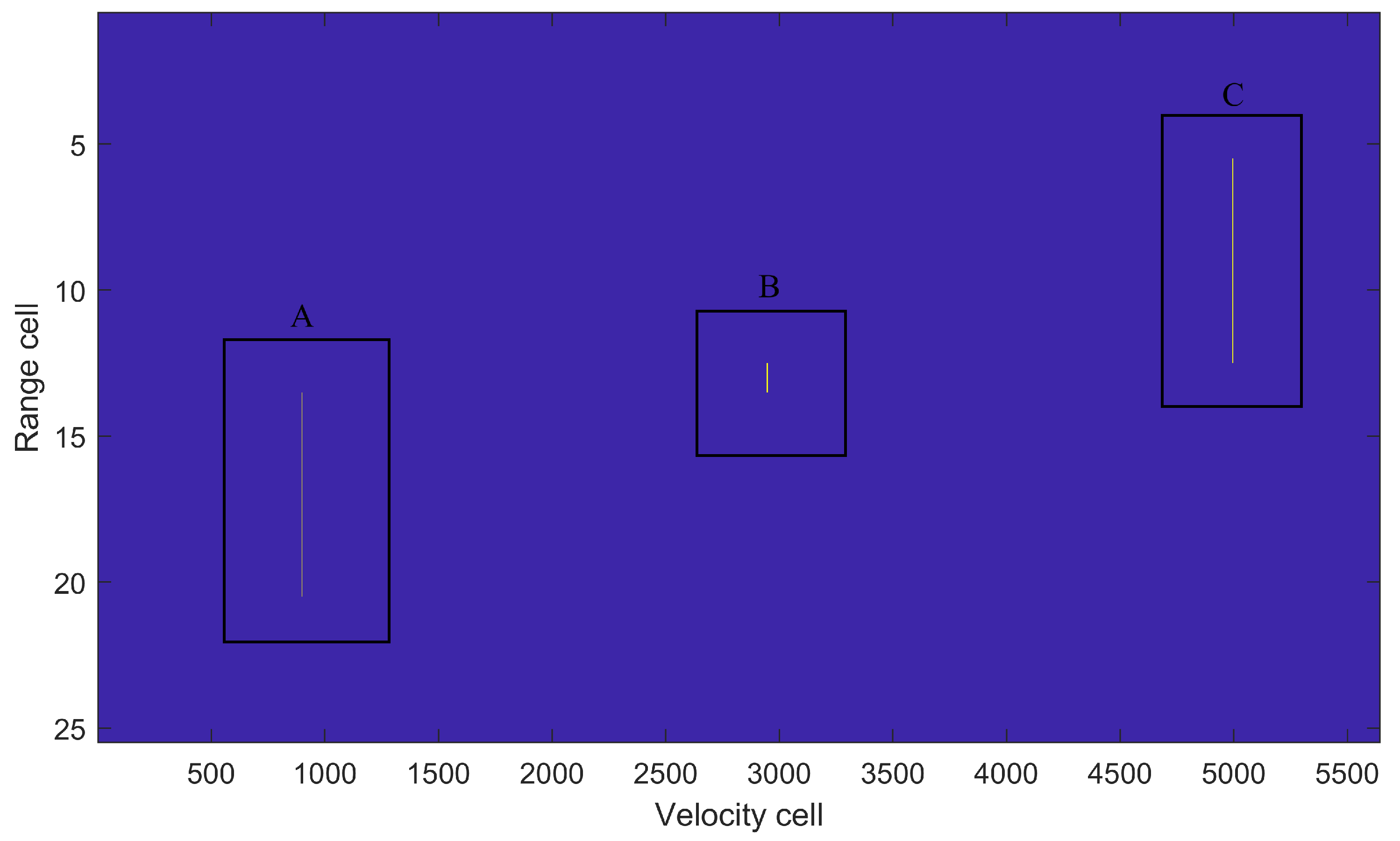
Figure 3 shows. A simulation result for an ERD plane with
is depicted in
Figure 4. The spikes in regions A, B, and C represent
,
, and
, respectively. When the folding factor is correctly matched (region B), the RM is minimized. Conversely, in cases where the folding factor is mismatched (regions A and C), the RM significantly increases.
Let represent the sampling interval, and the pulse length is given by . Consequently, the dimensions of the ERD plane are .
3. Improved SMC-PHD Filter
3.1. State Transition Model
In the PHD filter, the state of multiple targets can be modeled as an RFS. Therefore, at time
k, the state of
targets can be represented as:
where
represents the target’s index at time
k.
This tracking system utilizes a constant acceleration (CA) model, defining the target’s state vector as follows:
where
is the range,
is the baseband velocity,
is the ambiguity number,
is the acceleration, and
represents the intensity of the target.
Then, the state transition model of the target can be expressed as
where
denotes the rounding operator
.
,
,
, and
represent random variables following Gaussian distributions with zero mean and variances
,
,
, and
, respectively.
represents the uncertainty in the model during state transitions. In the CA model, it is commonly represented by the maximum value of the jerk.
denotes the power spectral density of noise in the target’s reflectivity.
and
signify the observation errors of the radar in the range and velocity dimensions, respectively.
3.2. Observation Model
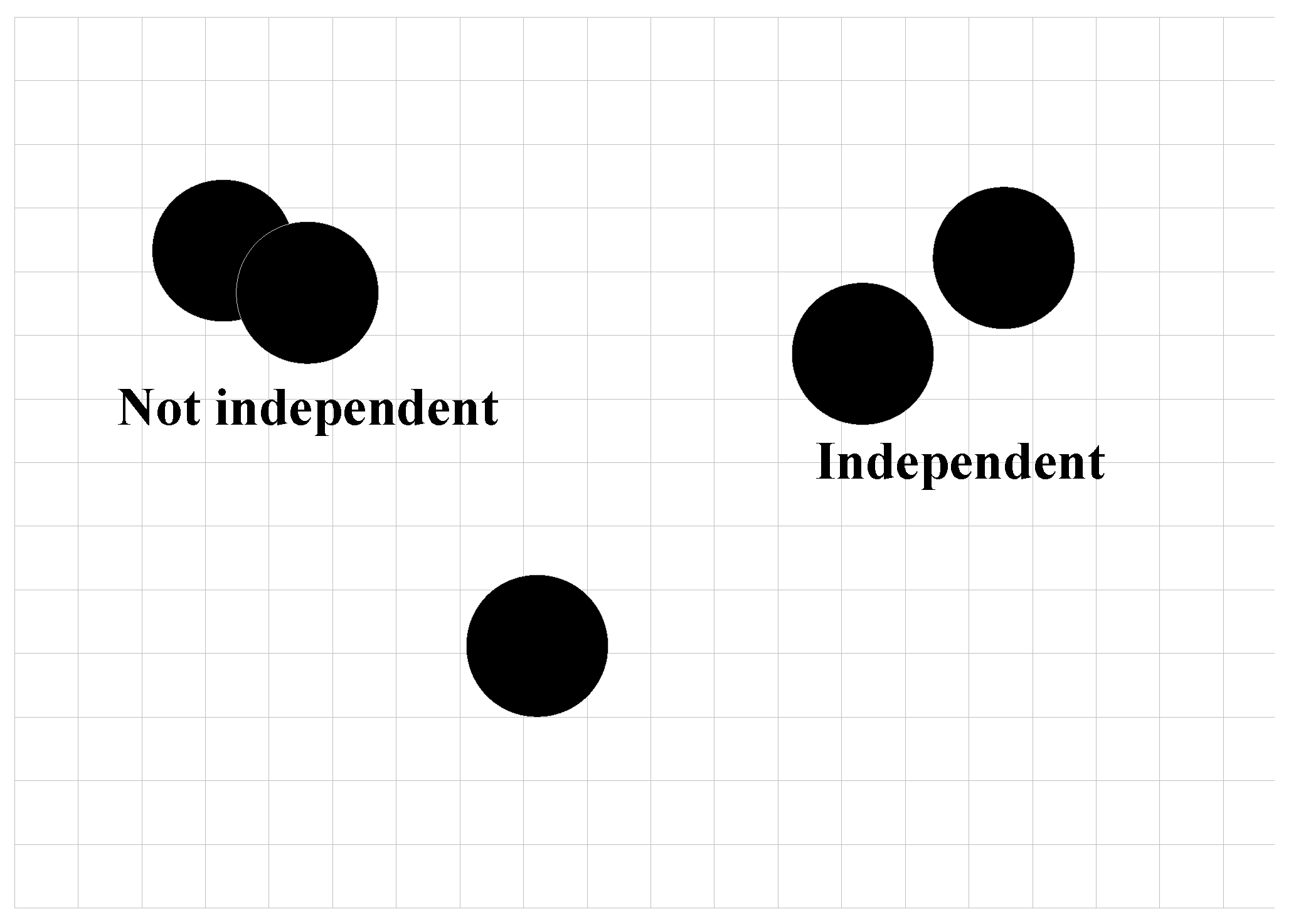
In the observation data, this paper assumes that the influence of all targets on the observations is non-overlapping, meaning that the targets are considered to be independent of each other. As depicted in
Figure 5, the black circles represent the influence range of a target. When the separation distance between targets is greater than the target’s influence range, these targets can be regarded as independent; otherwise, they are not considered independent.
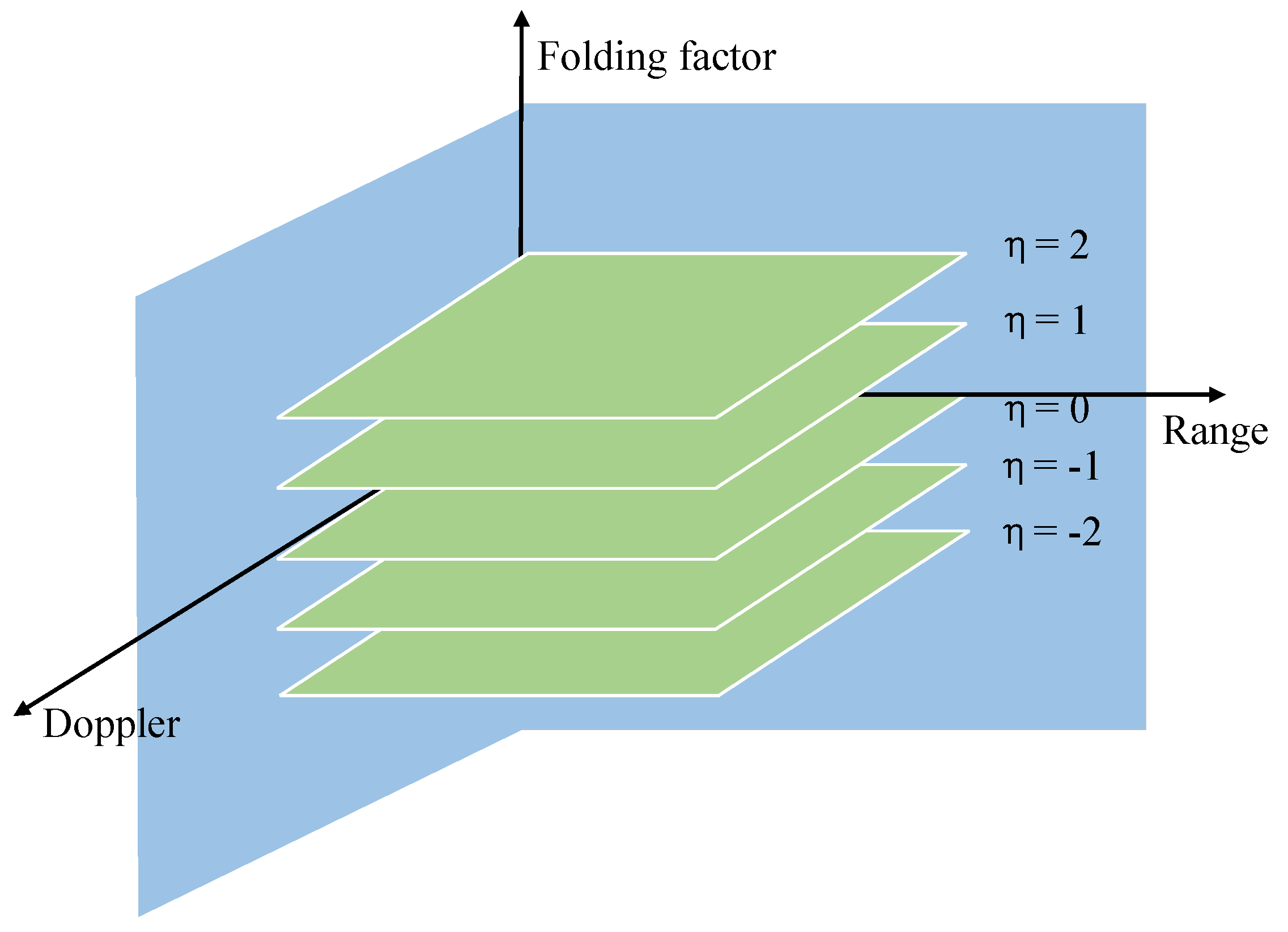
Based on the previous analysis, after performing the KT-MFP processing, different folding factors yield distinct SRD planes. In this paper, the SRD planes are stacked in order of folding factor values to form an FRD space, as illustrated in
Figure 6.
Therefore, after forming the FRD space, the measurement data consist of
cells, where
N is the number of range cells,
M is the number of Doppler cells, and
corresponds to the number of folding factors. This can be specifically described as
where
represents the observation value of the cell
at time
k, and it can be expressed as
where
indicates the situation where there are
targets, while
means there are no targets.
is the observation noise in the cell. Currently, some scholars use the point spread model (PSM) for research [
31], but when the target has acceleration, the PSM will no longer be applicable. To compensate the DFM for accelerated targets, we propose a new observation model named the line spread model (LSM), expressed in (
18) and (
19).
While
,
where the operator
is a logical operator that outputs the logical value “1” when the condition of the expression is true, and “0” otherwise.
and
are the length of each SRD cell in the range and the velocity axes.
is the diffusion coefficient.
and
represent the resolution cell.
Figure 7 shows an example of
.
Assuming statistical independence among measurement data in different resolution cells under the multi-target state condition, the likelihood function of the multi-target observation model can be derived as follows.
where
In the above equation, refers to the probability density function (PDF) describing the distribution of noise across the entire RD plane. represents the collection of resolution cells affected by the target.
For the mirror target, its observation model does not match the LSM proposed in this paper. Furthermore, the state of the mirror target does not match the motion model, and effective recursion cannot be formed. Therefore, in the FRD space, the likelihood ratio of the mirror target can be effectively suppressed and will not be greater than the likelihood ratio of the real target.
3.3. Adaptive Birth Particle Generation
For the TBD method based on SMC-PHD, it is necessary to approximate the true state distribution of targets using prior knowledge to generate birth particles. However, in real tracking scenarios, it is not possible to know the specific areas where targets may appear in advance. The traditional approach is to generate particles uniformly across the entire measurement area. However, this method has two drawbacks. First, it leads to inefficient use of particles, with many particles distributed in non-target areas, resulting in wastage of computational resources and poor real-time performance. Second, it is not conducive to the tracking of weak targets, as particles in regions with actual targets have lower effective weights, which can degrade the performance of the tracking filter.
Another novel approach is measurement-driven distribution, which uses measurement data to generate birth particle distribution. In [
32], particles are uniformly distributed in resolution cells where the measurement amplitude exceeds a certain preset threshold. Compared to traditional methods, this approach improves particle efficiency, although measurement information is still not fully utilized. In [
31], the target’s location within resolution cells is initially determined using measurement amplitude information, followed by likelihood computation of particles to obtain weights. Finally, adaptive birth particle generation is achieved through resampling based on particle weights. While this method fully utilizes measurement information, it requires additional computation of the particle likelihood ratio, which reduces computational efficiency. Addressing these issues, we propose a new method, namely, amplitude-based adaptive birth particle generation.
Specifically, assuming the number of birth particles is
L, the procedure involves first rapidly sorting measurements in descending order based on their amplitudes and selecting the top
L measurements. Subsequently, these measurements’ amplitudes are used as weights for resampling, where measurements with larger amplitudes are replicated more times. Finally, particles are uniformly distributed across the resolution cells corresponding to these measurements, achieving adaptive birth particle generation. The pseudo-code for this implementation is outlined as shown in Algorithm 1.
| Algorithm 1 Adaptive Birth Particle Generation Pseudo-Code |
Step 1: Initialization. L is the number of birth particles, is the collection of observations. is the i-th observation, is the amplitude of observation. , and is the range, velocity, and folding factor of the observation. Step 2: Sort according to amplitude, take the first L observations. “descend”) Step 3: Generate normalized weights using amplitudes. for end Step 4: Resampling. Step 5: Birth particle generation. for end where represents uniform distribution. represents the range and velocity resolutions, respectively. is the maximum acceleration, is the minimum amplitude, and is the maximum amplitude.
|
The proposed method has fewer steps compared to existing methods, resulting in a simpler implementation. Furthermore, it eliminates the need for likelihood ratio computations, significantly reducing computational complexity. This method also enhances particle utilization efficiency, enabling an effective approximation of the true target distribution, thus demonstrating higher engineering application value.
3.4. Implementation of SMC-PHD Filter
In multi-target Bayesian recursion, there is a significant computational challenge associated with set integrals. The PHD filtering algorithm based on RFS addresses this challenge by propagating the first-order moment of the posterior PDF of multiple targets, thereby simplifying the multi-target state space into a single-target state space and reducing computational complexity substantially. However, PHD recursion still involves high-dimensional integrals without closed-form expressions, and numerical integration encounters the “curse of dimensionality” issue [
33]. To overcome this problem, we can employ sequential Monte Carlo (SMC) methods using a weighted particle set
to propagate the posterior PHD of multiple targets. Specifically, the PHD
can be approximated as
where
is the Dirac delta function.
The SMC-PHD-TBD process includes prediction, update, resampling, and state extraction. In this process, only the birth and death of targets are considered, while target spawning is not taken into account. The specific algorithm flow is as follows:
Generate
surviving target particles and
birth target particles based on the proposal distribution
and birth distribution
.
The weight corresponding to the particle becomes
where
is the survival probability of the particle,
is the transition probability density, and
is the intensity of the birth target.
In the update step, it is necessary to utilize the measurements at time
k to update the weights of particles. Since raw data are used as measurements without any preprocessing, we can assume the detection probability
. Therefore, the updated weights can be expressed as
where
is the clutter normalization coefficient,
is defined in (
21),
is defined in (
22), and set
represents the collection of all predicted particles. Since
and
are both PDFs of noise, it can be assumed that
. Therefore, (
26) can be simplified to
To overcome the issue of particle degeneracy, it is necessary to perform resampling of the updated particles [
34]. Specifically, resampling is conducted on particle set
to obtain particle set
. As a resampling method with both performance and efficiency [
35], systematic resampling is applied in this paper.
The SMC-PHD filter requires the use of clustering algorithms to extract states, specifically to identify local maximum in the multi-target state space for target state estimation. However, in TBD scenarios, a single target can affect multiple resolution cells, which contradicts the assumption of the PHD filter that each target corresponds to a single measurement hypothesis. If traditional methods, assuming target number , are used to estimate the number of targets, it can lead to an overestimation of the target number by the filter. Furthermore, since the proposed method tracks targets in the FRD space, mirror targets can be misclassified as real targets, significantly affecting the target number estimation.
To address the problem of target number overestimation, we propose a method called particle space projection. As shown in
Figure 6, the FRD space is generated, and particles in the FRD space are projected onto the RD plane along the folding factor dimension. After projection, particles corresponding to mirror targets and real targets will occupy the same region. By applying density-based spatial clustering of applications with noise (DBSCAN) clustering to the particles on the RD plane, particles with different folding factors but similar range and Doppler characteristics can be grouped into the same cluster. This clustering approach eliminates the influence of mirror targets and targets spanning multiple resolution cells, thereby resolving the issue of target number overestimation.
It is worth noting that to mitigate the impact of mirror targets only the velocity and range information of particles was utilized. Therefore, particles with different folding factors could also be clustered into the same cluster. So, it is necessary to count the number of particles corresponding to each folding factor within a cluster, and then, assign all particles to the folding factor that has the highest proportion.
4. Results and Discussion
4.1. LSM Performance Simulation
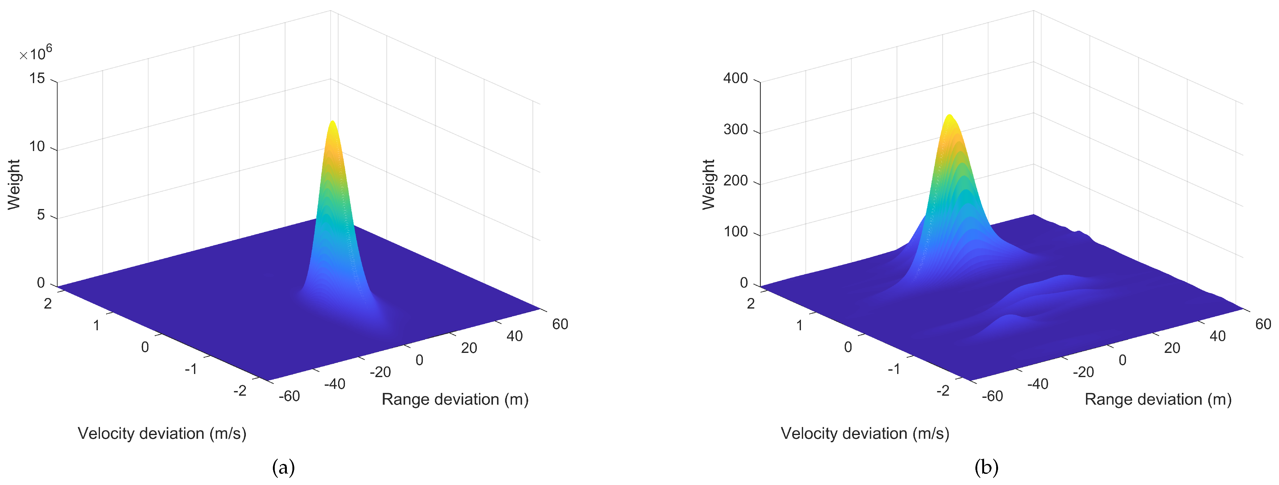
To evaluate the performance of LSM and PSM, we simulated a target with acceleration and computed the relationship between particle weights and the deviations of particle states from the target’s velocity and range, as shown in
Figure 8. It can be observed that at a given SNR of −21 dB, the weights of LSM are significantly higher than those of PSM, indicating that LSM performs better in target detection in the presence of DFM.
To verify the suppressive capability of LSM against mirror targets, we simulated a target with acceleration and the folding factor
. Setting the folding factor
, we obtained the result shown in
Figure 9 after KT-MFP processing. From the graph, it is evident that when the folding factor is matched (i.e.,
), the RM caused by velocity ambiguity has been compensated, i.e., DFM. However, when the folding factor is mismatched (i.e.,
), MFP exacerbates RM instead. Therefore, in the PHD-TBD process, the observation model of real targets matches well with LSM, resulting in higher weights. In contrast, mirror targets, whose observation model does not match LSM, exhibit lower weights.
Figure 10 presents simulation results consistent with the parameters and settings of
Figure 9, demonstrating the relationship between particle weights and the deviations of particle states from target velocity and distance when the folding factor
in LSM. From the graph, it is evident that particle weights are significantly higher for real targets, whereas they are much lower for mirror targets.
Furthermore, the state transition of real targets aligns with (
15), whereas that of mirror targets does not, resulting in their filtration by the filter. In summary, mirror targets do not impact the detection and tracking of targets.
4.2. Multi-Target Simulation Design
The echoes are generated by combining the signal with zero-mean Gaussian white noise and can be represented as
the variance in
is
.
Then, the SNR of the echoes is determined as
where
P is the power of signal:
The parameters of the radar are shown in
Table 1.
In the table above, we have set the folding factor value to
because this configuration extends the velocity range to −827.2 to 827.2 m/s, which meets the requirements for detecting most high-speed targets in practical engineering applications. The optimal sub-pattern assignment (OSPA) metric is employed to evaluate the performance of multi-target tracking [
36,
37]. We assess the performance of the tracker using the normalized deviations of the range and Doppler cell.
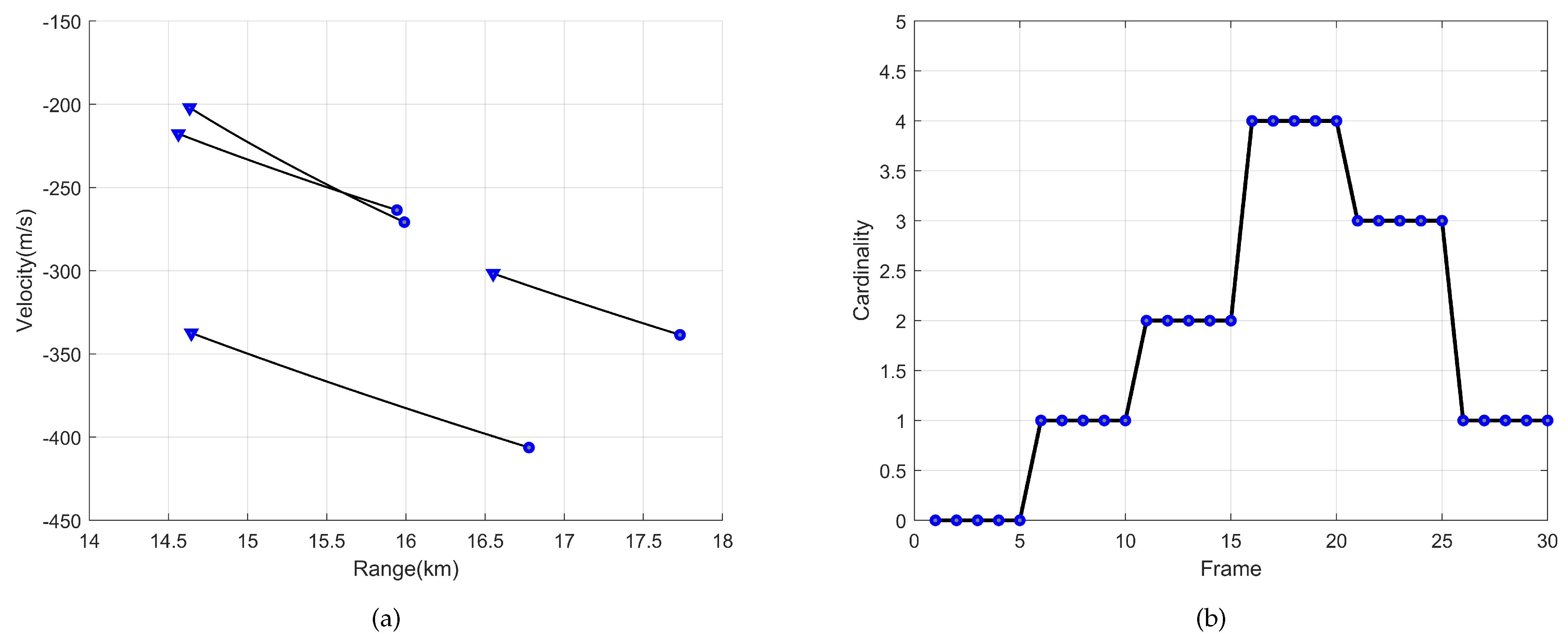
To validate the effectiveness of the algorithm, we designed four high-speed, high-maneuvering targets that included target appearances and disappearances. The target parameters are shown in
Table 2, and the multi-target simulation design is depicted in
Figure 11. The total detection time spans 30 frames, equivalent to 30 coherent processing intervals (CPIs), and the experiment performs 100 Monte Carlo simulations.
4.3. Method Comparison Experiment
To validate the performance of the proposed method, we conducted comparative experiments. Six different methods were selected for comparison, as detailed in
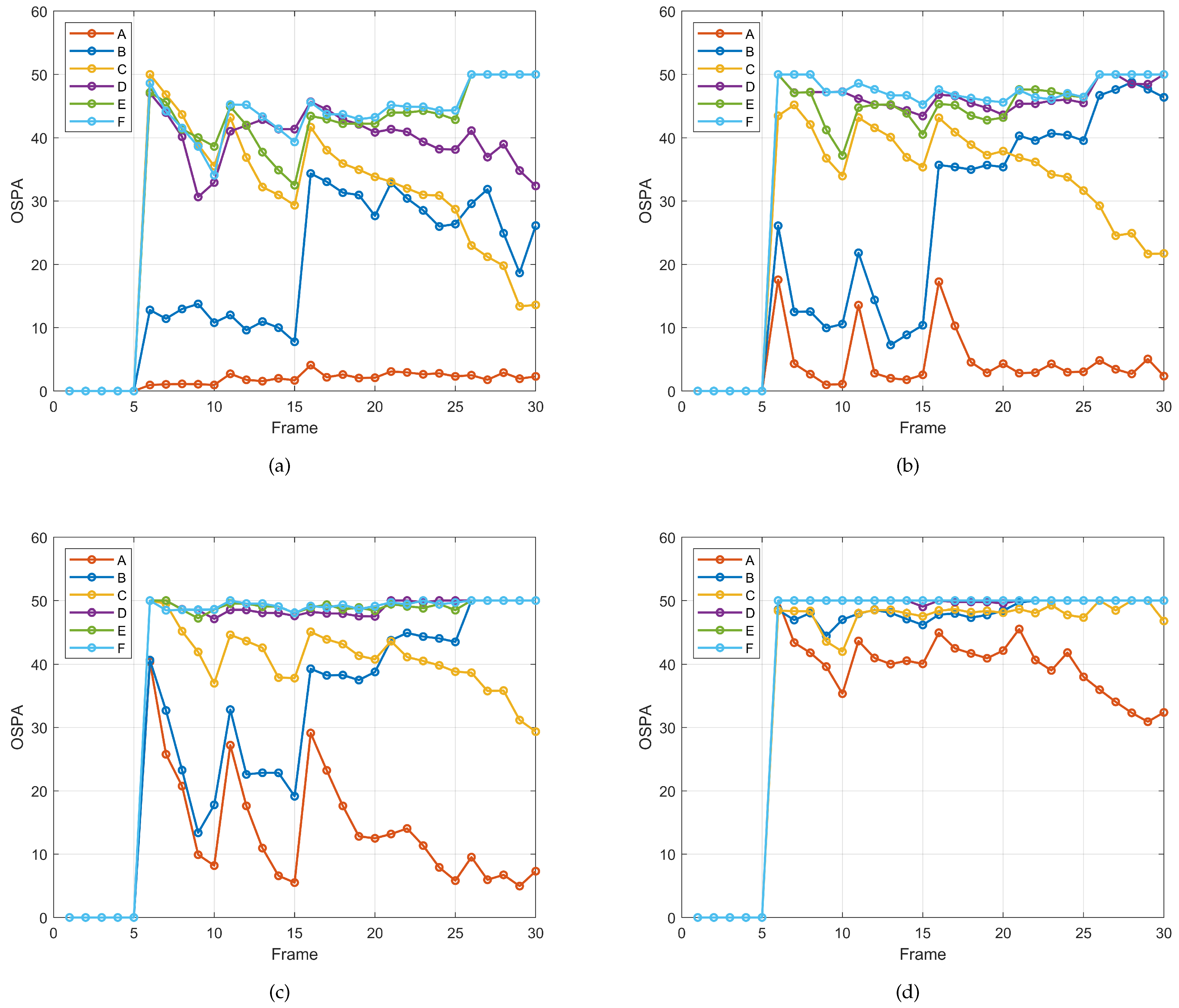
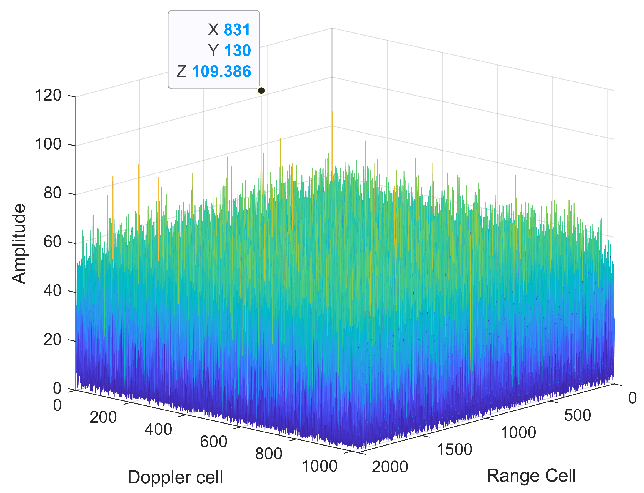
Table 3, with method A representing the proposed method. The experiments were conducted under four SNR conditions: −12 dB, −14 dB, −16 dB, and −18 dB. The ERD plane at the 20th frame was selected as an example, as shown in
Figure 12. It can be observed that the targets are almost completely submerged in noise, making it impossible to directly detect and track the targets using traditional DBT methods.
For the six methods mentioned above, we set the particle birth probability to 0.05 and the survival probability to 0.95. The number of birth particles was set to 2000, and the number of survival particles to 5000. For methods A, B, C, and D, the range for the birth particles was set to 10 km < < 20 km, −800 m/s < < 100 m/s, −15 m/s2 < < 15 m/s2, 30 < < 100. Methods E and F did not account for VA, so the velocity range for birth particles was set to −270 m/s < < 270 m/s. During state extraction, we first normalized the range and Doppler cells, then set the minimum radius for DBSCAN clustering, with a density threshold of 500. The OSPA metric is configured with an order and a cutoff parameter .
The results of the cardinality estimation are shown in
Figure 13, and the OSPA distances are shown in
Figure 14. For methods E and F, which did not account for VA and utilized PSM along with a uniform birth distribution, the coherent accumulation gain was low, resulting in poor filter performance. Consequently, these two methods performed the worst across the four SNR conditions and were generally unable to detect and track targets effectively.
Comparing methods B, C, and D demonstrated the effectiveness of the proposed LSM and adaptive birth particle generation methods. The comparison of method A with all other methods confirmed the superiority of the proposed method. It yielded cardinality estimates closest to the true values, achieved the smallest OSPA distances, and maintained robust detection and tracking performance even as the SNR decreased.
It is noteworthy that for an SNR of −12 dB, method B exhibited overestimation of cardinality in the first 15 frames due to significant interference from mirror targets in the PSM model. In the subsequent 15 frames, this method failed to detect targets, resulting in a sudden increase in OSPA. This was due to the appearance of two targets with VA, which the PSM could not effectively distinguish from real and mirror targets, leading to degraded algorithm performance. The proposed LSM effectively addressed these problems, remaining unaffected by mirror target interference.
As shown in
Table 4, the average running times for the six methods mentioned above at an SNR of −14 dB are listed, divided into LTCI and TBD processes. The simulations were conducted on a computer with an i7-12700F CPU, an RTX-3060ti GPU, and MATLAB version 2022a. The KT was implemented using the Chirp-Z Transform [
38].
From the table, it is evident that the additional computational load of LSM compared to PSM (methods A and B) is negligible. The increase in computational load due to the adaptive birth particle generation (methods A and C) is acceptable, achieving a excellent performance-to-efficiency ratio. Methods E and F have shorter LTCI times because they do not consider VA. For methods A, B, C, and D, achieving a threefold increase in velocity range only results in a linear increase in computational complexity. During the TBD process, method A, compared to method D, incorporates LSM, adaptive birth distribution, and particle space projection. While significantly enhancing target detection and tracking performance, the added computation time remains within an acceptable range. Overall, the proposed KT-MFP-ISMC-PHD-TBD method significantly enhances algorithm performance without imposing substantial computational burdens, making it an effective and efficient method.
4.4. Ubiquitous Radar Actual Data Validation
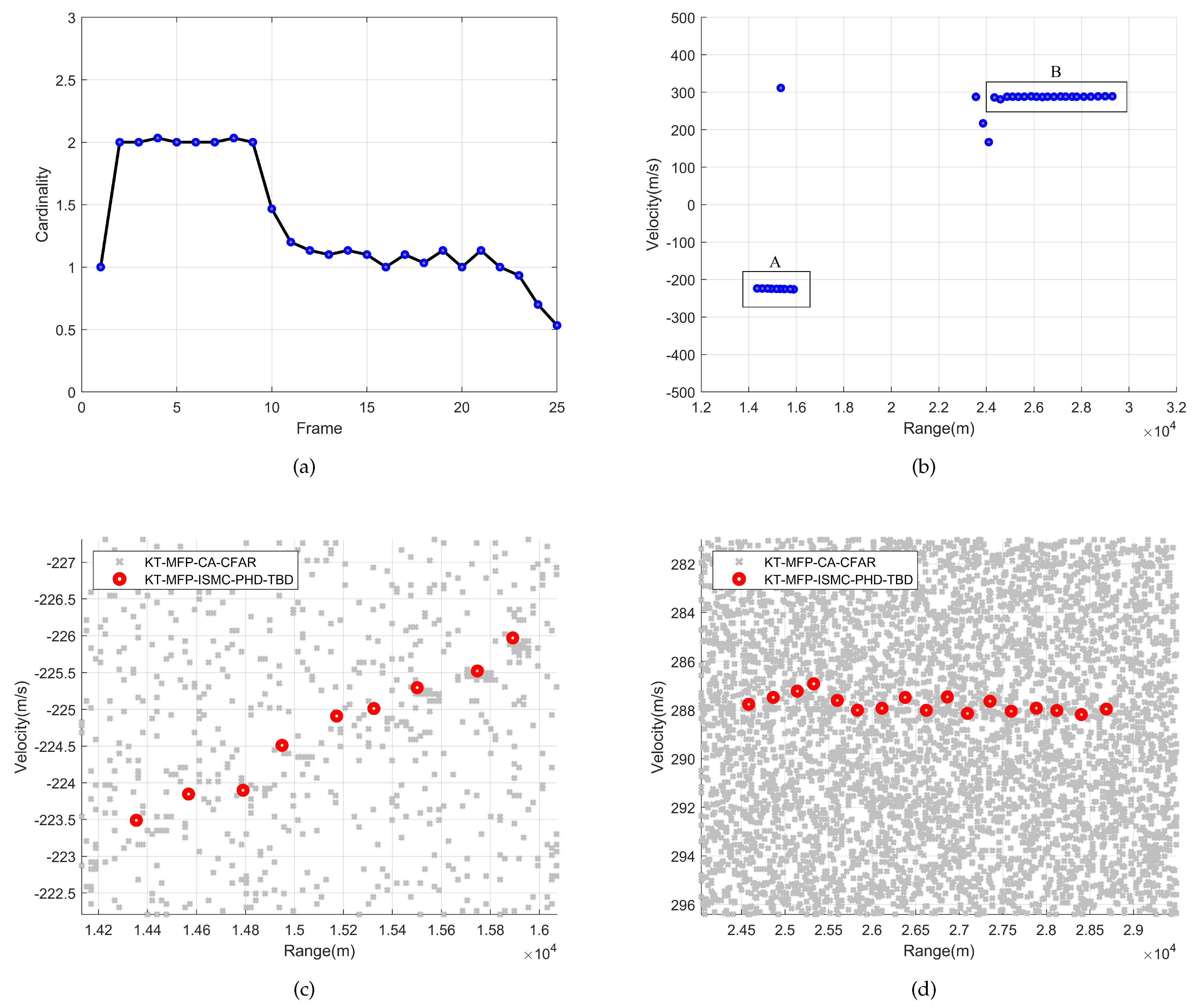
In this section, we validate the proposed method using actual data collected by a ubiquitous radar system targeting multiple high-speed, highly maneuverable targets. Specifically, the collected echo data consist of 25 frames of radar detection data for two civil aviation aircraft, as shown in
Figure 15. One aircraft has a relatively prominent peak in the RD plane, but with a low SNR, while the other aircraft is submerged in noise and clutter. The parameters of the ubiquitous radar system are consistent with those in
Table 1. In the algorithm, the coverage range for birth particles is set to 10 km <
< 30 km, −400 m/s <
< 400 m/s, −5 m/s
2 <
< 5 m/s
2, 40 <
< 140. Other parameters remain consistent with those in
Section 4.3.
Figure 16 illustrates the results of the algorithm’s detection and tracking.
Figure 16a shows the cardinality estimation result, where it can be observed that there are two targets in the first ten frames, after which one target disappears. This result demonstrates the algorithm’s performance in scenarios with changing target numbers.
Figure 16b presents the trajectory estimation results, where the speed of Target A is approximately −200 m/s, and the speed of Target B is around 300 m/s. To highlight the filtering effect for high-speed, highly maneuverable targets during the TBD process, we conducted a comparative experiment using the KT-MFP-CA-CFAR method (
), with the results shown in
Figure 16c,d. From these figures, it is evident that target A exhibits acceleration, while target B maintains a steady speed. The experimental results with actual data confirm that the proposed method can effectively detect and track multiple high-speed, highly maneuverable targets.
5. Conclusions
Ubiquitous radar transmits a low-gain, wide-beam signal, necessitating a strategy of time-for-energy trade-off to enhance target detection capability through LTCI. However, the presence of multiple high-speed, highly maneuverable targets can introduce RM, DFM, and VA, which severely degrade LTCI performance. To address these challenges, this paper proposes the KT-MFP-ISMC-PHD-TBD method. Initially, KT compensates for first-order RM, and MFP compensates for VA, allowing different folding factors to be stitched into an ERD plane, thereby achieving a larger velocity range. Additionally, the continuous spatial coverage capability of ubiquitous radar is well suited for recursive TBD algorithms. Therefore, we propose an improved SMC-PHD method, utilizing amplitude-based adaptive particle birth and employing LSM to compensate for DFM. Ultimately, the method eliminates mirror target interference through particle space projection, enabling joint detection and estimation of multiple targets.
The simulation results demonstrate that LSM is more suitable than PSM for accelerating targets and effectively suppresses mirror target interference. In comparative experiments, the proposed method exhibits superior performance over traditional methods and maintains robust performance even as the SNR decreases. In terms of computational efficiency, the TBD process did not impose a significant computational burden. It achieved a larger velocity range while only increasing the computational complexity linearly, effectively balancing performance and efficiency. Finally, actual ubiquitous radar data confirm the proposed method’s ability to detect and track multiple high-speed, highly maneuverable targets.
