Cruise Speed Model Based on Self-Attention Mechanism for Autonomous Underwater Vehicle Navigation

Abstract

This study proposes a cruise speed model based on the Self-Attention mechanism for speed estimation in Autonomous Underwater Vehicle (AUV) navigation systems. By utilizing variables such as acceleration, angle, angular velocity, and propeller speed as inputs, the Self-Attention mechanism is constructed using Long Short-Term Memory (LSTM) for handling the above information, enhancing the model’s accuracy during persistent bottom-track velocity failures. Additionally, this study introduces the water-track velocity information to enhance the generalization capability of the network and improve its speed estimation accuracy. The sea trial experiment results indicate that compared to traditional methods, this model demonstrates higher accuracy and reliability with both position error and velocity error analysis when the used Pathfinder DVL fails, providing an effective solution for AUV combined navigation systems.

1. Introduction

Recently, interest in marine resources has grown considerably, resulting in increased marine development activities. Autonomous Underwater Vehicles (AUVs) are crucial for tasks such as seabed resource exploration, submarine pipeline maintenance, and marine data collection [1,2]. Therefore, obtaining precise navigation and positioning technology for AUVs is crucial to ensuring successful and timely task completion, owing to the highly complex marine environment. In contrast to land robots [3] and aerial robots [4], AUVs do not receive GPS signals underwater, posing a challenge for traditional satellite-dependent navigation techniques in this environment. Emerging technologies have been increasingly employed recently for successful underwater localization and navigation. The primary underwater navigation and localization techniques are categorized into four main groups: acoustic navigation [5,6,7], geophysical navigation [8,9,10], Simultaneous Localization and Mapping (SLAM), and inertial navigation and dead reckoning [11,12]. Acoustic waves are the most effective method for transmitting information underwater, making acoustic navigation the primary method for underwater target navigation and localization. Nonetheless, the acoustic beacons must be placed in advance, as acoustic navigation is ineffective in an unknown environment. Geophysical navigation can be divided into three primary groups based on the requisite geophysical parameters: terrain-matching navigation, marine geomagnetic navigation, and gravity navigation. However, geophysical navigation is limited by the requirement to obtain geophysical parameters in advance. Conversely, SLAM enables AUVs to create maps of their surroundings and determine their position within that environment. However, SLAM requires external environmental information measured by additional sensors and high computation capacity.

Inertial navigation is an autonomous system known for not relying on external information or emitting energy externally. The Inertial Navigation System (INS) uses triaxial gyroscopes and accelerometers to measure angular rate and acceleration. Then, the attitude, velocity, and position information of the AUV is calculated by an integral operation. However, the integration process results in error accumulation in the INS, and over a long navigation period, the position can be shifted considerably. This approach partially mitigates the error accumulation problem by utilizing a Doppler Velocity Logger (DVL) for bottom-track velocity and integrating INS and DVL measurements. Kalman filtering (KF) is a widely applied data fusion method [13], and it can achieve optimal filtering with Gaussian white noise in the system process. The bottom-track velocities measured by the DVL are indispensable in the data fusion algorithm. However, the DVL is sensitive to the complex marine environment, which may cause inaccuracies in velocity measurements. For instance, DVL bottom tracking can be vulnerable to interference and disruptions due to steep seafloor slopes or rifts, AUV attitude, currents, and fish populations [14], as shown in Figure 1. In cases where the DVL produces anomalous values for a brief period, the issue can be resolved by utilizing effective bottom tracking from the previous moment. Nevertheless, this method is inadequate when the DVL outputs anomalous data for an extended period or is inactive, in which case the INS solution error accumulates and the navigation accuracy significantly degrades over time. Consequently, investigating the navigation method when the DVL output remains invalid for an extended period is crucial.

Figure 1. Vulnerability to bottom-track interference.

Some methods have been commonly used in the existing literature to address invalid bottom tracking [15,16]: One approach involves implementing combined navigation by installing additional sensors to replace the DVL in case of failure; however, this method increases costs and system complexity. Conversely, another method replaces the DVL with a mathematical model generating virtual bottom velocity information, solved by way of modeling single- and three-degree-of-freedom dynamics [17]. And Kinsey et al. developed a single-degree-of-freedom nonlinear dynamic model estimator and verified its feasibility [18]. Zhao et al. introduced a mechanism for outlier detection in DVL data and compensated for velocity anomalies using a kinematic model. However, the complexity of AUV models in challenging marine environments makes it difficult to obtain accurate hydrodynamic parameters. Therefore, building precise AUV dynamic models is evidently impractical. Establishing dynamic models with single and three degrees of freedom, validated through sea trials, demonstrated that the speeds calculated using these models closely aligned with those measured by the DVL.

Various machine learning algorithms, such as Support Vector Machines (SVMs) [19], Random Forests (RFs) [20], Extreme Learning Machines (ELMs) [21], and Artificial Neural Networks (ANNs) [22], have been employed in diverse fields owing to the recent widespread application of artificial intelligence technology. In their study, Mu et al. [23] applied the time-series learning mechanism to AUV navigation and proposed a novel neural network framework using Long Short-Term Memory (LSTM) to process multi-sensor data and determine the position of an AUV during navigation. Another study [19] developed a hybrid predictor by combining partial least squares regression and support vector regression to estimate the bottom velocity of a DVL when faced with DVL failure. Lv et al. employed ELM to establish a model relationship between the AUV’s thruster speed, attitude, rudder information, and bottom velocity to compensate for DVL failures. Li et al. proposed a nonlinear autoregressive framework with heteroscedastic inputs (NARX) and adaptive Kalman filtering to predict and fuse DVL outputs. Water-track velocity and flow rate estimation during anomalous DVL bottom velocity were also investigated [24]. Our study presents a deep learning framework incorporating LSTM and Self-Attention to address this issue, considering the current velocity as a variable to estimate the water-track velocity of the DVL. The effectiveness of our approach is validated by comparing the results with the measured data.

This paper proposes a cruise speed model based on the Self-Attention mechanism for estimating AUV speeds in complex marine environments. Utilizing inputs like acceleration, angle, angular velocity, and propeller speed, the model estimates cruise speed via the Self-Attention mechanism. This cruise speed corresponds to the velocities along the three axes of the AUV onboard coordinate system. As a consequence, the model sustains high navigation accuracy even when the bottom-track velocity data are consistently unavailable. The main contributions of this paper are as follows:

(1) To address the continuous failure of bottom-track velocity measurements in complex marine environments, a deep learning-based AUV speed estimation model is constructed to predict and output bottom-track velocities, enhancing AUV navigation accuracy during DVL failures.

(2) LSTM will be used to separately extract time-series data from different data sources, and Self-Attention will be employed to enhance the encoding of time-series data. Water flow rate information is introduced into the network as input to compensate for ocean current information, increasing the model’s generalization capability.

(3) The proposed Self-Attention-based cruise speed model’s effectiveness on AUVs will be validated through sea trials and simulation data. The results show that the proposed model achieves better navigation accuracy compared to using water-track velocity compensation.

The rest of this paper is organized as follows: Section 2 describes the AUV and equipment specifications used for the field trials. Section 3 derives a model for the application of Kalman filtering in combined AUV navigation. Section 4 details the network model framework and analyzes the results obtained in Section 5. Finally, Section 6 concludes the study.

2. An Introduction of the AUV Platform

Herein, we present the AUV used in our experiment, depicted in Figure 2. The XH R300 employs a double main thrust propulsion system capable of attaining a maximum speed of 5 knots and sustaining continuous travel for up to 10 km. The hydrodynamic characteristics of the XH R300 are notably intricate, necessitating the formulation of a three-degree-of-freedom dynamics model to elucidate its motion. This modeling endeavor is predicated on several key assumptions: first, the AUV is treated as a rigid body; second, the current is assumed to be a two-dimensional flow lacking rotational components; and third, the fluid medium is regarded as uniform and unbounded. The kinetic equations governing the AUV’s motion are conventionally expressed as follows:

$$M\stackrel{·}{v}+C\left(v\right)v+D\left(v\right)v=f$$

(1)

where v denotes the triaxial component of the AUV velocity in the carrier coordinate system, M and C, respectively, denote the inertia matrix and the Coriolis centripetal matrix of the rigid body, $f=\left[{\left(\tau \right)}_X,{\left(\tau \right)}_Y,{\left(\tau \right)}_N\right]$ are external forces and moments, ${\left(\tau \right)}_X$ and ${\left(\tau \right)}_Y$ are, respectively, the axial and lateral forces acting on the AUV, and ${\left(\tau \right)}_N$ is the yaw external moment. The expression is as follows:

$$f=\left[\begin{array}{c}{\tau }_X\\ {\tau }_Y\\ {\tau }_N\end{array}\right]=\left[\begin{array}{c}{T}_{port}+T_{stbd}\\ 0\\ \left(T_{port}-T_{stbd}\right)B/2\end{array}\right]$$

(2)

where $T_{port}$ and $T_{stbd}$ are, respectively, the thrust of the port and starboard thrusters, and B is the distance between the thrusters. The three-degree-of-freedom nonlinear dynamics model of the AUV can be described as

$$\begin{array}{cc}\hfill & {\tau }_X=\left(m-X_{\dot{u}}\right)\dot{u}-m\left(x_G{r}^2+vr\right)+Y_{\dot{v}}vr+\frac{Y_{\dot{r}}+N_{\dot{v}}}{2}{r}^2+X_{u}u+X_{\left|u\right|u}\left|u\right|u\hfill \\ \hfill & {\tau }_Y=\left(m-Y_{\dot{v}}\right)\dot{v}+\left(m{x}_G-Y_{\dot{r}}\right)\dot{r}+\left(m-X_{\dot{u}}\right)ur+Y_{v}v+Y_{r}r+Y_{\left|v\right|v}\left|v\right|v+Y_{\left|r\right|r}\left|r\right|r\hfill \\ \hfill & {\tau }_N=\left(m{x}_G-N_{\dot{v}}\right)\dot{v}-\left(I_{zz}-N_{\dot{r}}\right)\dot{r}+m{x}_{G}ur-Y_{\dot{v}}uv-\frac{Y_{\dot{r}}+N_{\dot{v}}}{2}ur+X_{\dot{u}}uv+N_{v}v\hfill \\ \hfill & +N_{r}r+N_{\left|v\right|v}\left|v\right|v+N_{\left|r\right|r}\left|r\right|r\hfill \end{array}$$

(3)

where $X_{(·)}$, $Y_{(·)}$, and $N_{(·)}$ represent hydrodynamic coefficients. According to Equations (2) and (3), the AUV speed is related to the acceleration, angle, angular velocity, and amount of rudder thrust. The thrust of the servos, in turn, is related to the rotational speed and current obtained through various sensor measurements, which will be used later in this study to estimate the AUV speed. The equipment used to obtain the relevant data is illustrated below.

Figure 2. Basic structure of XH R300.

The XH R300 is equipped with a signal cabin, control cabin, power control cabin, and power operation cabin. The primary sensors include a GPS module, Iridium satellite, radio, Wifi, INS, DVL, and depth gauge to obtain AUV position, acceleration, angle, and angular velocity information. Based on functionality, the main control can be divided into a control unit, navigation and positioning unit, guidance and planning unit, perception unit, fault detection unit, and data storage unit. The navigation and positioning unit is crucial for real-time acquisition of AUV pose information and provides the foundational support for the operation of the control unit and guidance and planning unit. The GPS module offers real-time precise latitude and longitude data while the AUV operates on the water surface, as delineated in Table 1. Nevertheless, owing to the rapid attenuation of GPS signals in water, the XH R300 incorporates the INS (detailed in Table 2) that derives the AUV’s position, velocity, and triaxial attitude angle by integrating data from the gyroscope, measuring angular rates, and the accelerometer, gauging triaxial accelerations. However, the integration process inevitably results in error accumulation within the INS, impinging upon navigation accuracy. Consequently, the XH R300 is outfitted with a Pathfinder 600 KHz DVL developed by Teledyne, described in Table 3, to rectify these discrepancies. The DVL emits sound waves via a transducer when a phased array is employed, which, upon reaching the seabed, bounce back, enabling velocity estimation relative to the seafloor by analyzing frequency shifts in the received echoes. When GPS signals are unavailable underwater, the disparity between the raw speed of the INS and the speed of the DVL serves as feedback, refining the INS output through an indirect approach.

Table 1. GPS module specifications.

Equipment Type	GPS Module
Single-point positioning accuracy	<1.5 m
Velocimetry accuracy	0.03 m/s
Maximum data update frequency	1 Hz

Table 2. INS specifications.

Equipment Type	INS
Heading accuracy	0.5°
Attitude accuracy	0.02°
Gyro accuracy	0.05°/h (1$\sigma$)
Plus meter accuracy	200 $\mathsf{\mu }$g (1$\sigma$)

Table 3. DVL specifications.

Equipment Type	DVL
Maximum height	89 m
Minimum height	0.2 m
Speed range	±9 m/s
Resolution	0.1 cm/s
Pinging frequency	12 Hzmax

However, in deep-sea environments exceeding the operational range of the DVL or encountering steep seabed inclines, the acoustic waves of the DVL may fail to reach or be detected upon seabed contact, rendering the bottom-track data invalid and precluding its integration with INS for high-precision navigation. Although the DVL can also provide water-track velocities, they are notably less precise than bottom-track velocities and fail to meet stringent navigation accuracy requisites. A novel solution addressing these challenges is proposed herein and elaborated upon subsequently. Additionally, a depth gauge ISD4000 developed by Impact Subsea is integrated into the XH R300 for precise depth determination, ensuring accurate depth measurement.

3. AUV Combined Navigation Model

The combined AUV navigation model outlined in this section primarily relies on integrating the INS and DVL systems. Initially, the INS error model is used to formulate the state equations of the integrated navigation system. Subsequently, data gathered by the INS facilitate AUV motion prediction. Observations from the INS and DVL are then incorporated into the model, refining its predictions to align more closely with actual values. This iterative process, conducted in the time domain, culminates in achieving combined AUV navigation. This section details the model construction process and the updated predicted values, which constitute a pivotal aspect of the process.

Model Construction

This study employs two coordinate systems: the navigation and carrier coordinate systems. The navigational coordinate system, denoted as $O-X^n{Y}^n{Z}^n$, situates its origin at sea level, with the $O{X}^n$ axis pointing northward, the $O{Y}^n$ axis eastward, and the $O{Z}^n$ axis directed toward the geocentric North-East Earth (NEU) geographical coordinates. Conversely, the carrier coordinate system, denoted as $O-X^b{Y}^b{Z}^b$, positions its origin at the center of gravity of the AUV, with the $O{X}^b$ axis directed forward, the $O{Y}^b$ axis starboard, and the $O{Z}^b$ axis downward. The navigational coordinate system undergoes three rotational transformations with respect to the carrier coordinate system: the heading angle $\alpha$ around the $O{Z}^n$ axis, the pitch angle $\beta$ around the $O{Y}^n$ axis, and the roll angle $\gamma$ around the $O{X}^n$ axis. Typically, instruments are situated in the carrier coordinate system. Therefore, to determine the AUV’s absolute position in the navigation coordinate system, the various AUV states are multiplied by its rotation matrix $C_b^n$, defined as follows:

$$C_b^n=\left[\begin{array}{ccc}cos\gamma cos\alpha -sin\gamma sin\beta sin\alpha & -sin\alpha cos\beta & cos\gamma sin\alpha +sin\alpha sin\beta sin\gamma \\ sin\gamma cos\alpha +cos\gamma sin\beta sin\alpha & cos\beta cos\alpha & sin\gamma sin\alpha -cos\gamma sin\beta cos\alpha \\ -cos\beta sin\gamma & sin\beta & cos\gamma cos\beta \end{array}\right]$$

(4)

In the navigation system, the navigation parameter errors of INS are selected as state variables. Due to the generally small error values, the state equation can be considered a first-order linear system, with the speed difference between INS and DVL used as the measurement variable. The error amount is then optimally estimated through standard Kalman filtering to feedback and correct the INS output. Leveraging the INS error model, the state vectors are identified as 15-dimensional error quantities of the INS, including attitude error ${\varphi }_E,{\varphi }_N,{\varphi }_U$, velocity error $\delta v_E,\delta v_N,\delta v_U$, position error $\delta p_E,\delta p_N,\delta p_U$, gyro zero bias ${\epsilon }_x,{\epsilon }_y,{\epsilon }_z$, and accelerometer zero bias ${\nabla }_x,{\nabla }_y,{\nabla }_z$.

$$X={\left[{\varphi }_E,{\varphi }_N,{\varphi }_U,\delta v_E,\delta v_N,\delta v_U,\delta p_E,\delta p_N,\delta p_U,{\epsilon }_x,{\epsilon }_y,{\epsilon }_z,{\nabla }_x,{\nabla }_y,{\nabla }_z\right]}^{\mathrm{T}}$$

(5)

The state equation of the system is as follows:

$$\stackrel{·}{X}=FX+W$$

(6)

where F is the state transfer matrix and W is the state noise. The system error propagation equation is shown as follows:

$$\left\{\begin{array}{c}\dot{\delta }L=-\frac{V_N}{{(R_M+h)}^2}\delta h+\frac{1}{R_M+h}\delta V_N\hfill \\ \dot{\delta }\lambda =\frac{V_{E}tanLsecL}{R_N+h}\delta L-\frac{V_{E}secL}{{(R_N+h)}^2}\delta h+\frac{secL}{R_N+h}\delta V_E\hfill \\ \dot{\delta }h=\delta V_U\hfill \\ \dot{\delta }{V}_E=(2\Omega V_{N}cosL+\frac{V_E{V}_N{sec}^{2}L}{R_N+h}+2\Omega V_{U}sinL)\delta L+\frac{V_E{V}_U-V_N{V}_{E}tanL}{{(R_N+h)}^2}\delta h\hfill \\ +\frac{V_{N}tanL-V_U}{R_N+h}\delta V_E+(2\Omega sinL+\frac{V_{E}tanL}{R_N+h})\delta V_N-(2\Omega cosL+\frac{V_E}{R_N+h})\delta V_U\hfill \\ +f_N{\phi }_U-f_U{\phi }_N+{\nabla }_E\hfill \\ \dot{\delta }{V}_N=-(2\Omega V_{E}cosL+\frac{V_E{sec}^{2}L}{R_N+h})\delta L+(\frac{V_E{tan}^{2}L}{{(R_N+h)}^2}+\frac{V_N{V}_U}{{(R_M+h)}^2})\delta h\hfill \\ -(2\Omega sinL+\frac{V_{E}tanL}{R_N+h})\delta V_E-\frac{V_U}{R_M+h}\delta V_N-\frac{V_N}{R_M+h}\delta V_U\hfill \\ +f_U{\phi }_E-f_E{\phi }_U+{\nabla }_N\hfill \\ \dot{\delta }{V}_U=-2\Omega V_{E}sinL\delta L-\left[\frac{V_E^2}{{(R_N+h)}^2}+\frac{V_N^2}{{(R_M+h)}^2}\right]\delta h+(2\Omega cosL+\frac{V_E}{R_N+h})\delta V_E\hfill \\ +\frac{V_N}{R_M+h}\delta V_N+f_E{\phi }_N-f_N{\phi }_E+{\nabla }_U\hfill \\ {\dot{\phi }}_E=\frac{V_N}{{(R_M+h)}^2}\delta h-\frac{1}{R_M+h}\delta V_N+(\Omega sinL+\frac{V_E}{R_N+h}tanL){\phi }_N\hfill \\ -(\Omega cosL+\frac{V_E}{R_N+h}){\phi }_U-{\epsilon }_E\hfill \\ {\dot{\phi }}_N=-\Omega sinL\delta L+\frac{V_E}{{(R_N+h)}^2}\delta h+\frac{1}{R_N+h}\delta v_E-(\Omega sinL+\frac{V_E}{R_N+h}tanL){\phi }_E\hfill \\ -\frac{V_N}{R_M+h}{\phi }_U-{\epsilon }_N\hfill \\ {\dot{\phi }}_U=(\Omega cosL+\frac{V_E}{R_N+h}{sec}^{2}L)\delta L-\frac{V_{E}tanL}{{(R_N+h)}^2}\delta h+\frac{tanL}{R_N+h}\delta V_E\hfill \\ +(\Omega cosL+\frac{V_E}{R_N+h}){\phi }_E+\frac{V_N}{R_M+h}{\phi }_N-{\epsilon }_U\hfill \end{array}\right.$$

(7)

The measurement equation for combined navigation is as follows:

$$Z=HX+V$$

(8)

where H is the measurement matrix and V is the measured noise.

The error equation for the DVL in the navigation coordinate system is as follows:

$$\begin{array}{cc}\hfill {\stackrel{\sim }{V}}_{dvl}^n& ={\stackrel{\sim }{C}}_b^n{C}_d^b{V}_{dvl}^d\hfill \\ \hfill & =\left[I-\psi \times \right]C_b^n{C}_d^b{V}_{dvl}^d\hfill \\ \hfill & =V_{dvl}^n-\psi \times V_{dvl}^n\hfill \\ \hfill & =V_{dvl}^n+V_{dvl}^n\times \psi \hfill \\ \hfill \delta V_d^n& ={\stackrel{\sim }{V}}_{dvl}^n-V_{dvl}^n=V_{dvl}^n\times \psi \hfill \end{array}$$

(9)

where $C_d^b$ denotes the rotation matrix from the DVL instrument coordinate system to the carrier coordinate system. We take the difference between the SINS and DVL velocities as the measure and construct the measure model according to the error model of the DVL as follows:

$$\begin{array}{cc}\hfill Z& ={\stackrel{\sim }{V}}_b^n-{\stackrel{\sim }{V}}_d^n=\left(V^n+\delta V_b^n\right)-\left(V^n+\delta V_d^n\right)\hfill \\ \hfill & =\delta V_b^n-\delta V_d^n=\delta V_b^n-V_d^n\times \psi \hfill \\ \hfill & =HX+V\hfill \end{array}$$

(10)

The specific form of H is as follows:

$$H=\left[\begin{array}{cc}\begin{array}{cccccc}0& {V_d^n}_U& -{V_d^n}_N& 1& 0& 0\\ -{V_d^n}_U& 0& {V_d^n}_E& 0& 1& 0\\ {V_d^n}_N& -{V_d^n}_E& 0& 0& 0& 1\end{array}& 0_{3\times 9}\end{array}\right]$$

(11)

where ${V_d^n}_E$, ${V_d^n}_N$, and ${V_d^n}_U$, respectively, denote the triaxial components of the DVL-measured velocity in the geographic coordinate system. Here, the combined SINS/DVL navigation model construction is completed.

4. Deep Learning Navigation Architecture

The AUV state data, captured as a time series, exhibit significant correlations over time. Previous studies on DVL anomalies often treated sensor data at each moment in isolation, neglecting the time-series correlations. Furthermore, not all data points are equally important in predicting subsequent states. In response to these considerations, this section presents a detailed description of a novel deep learning network architecture, developed after comprehensively examining these two aspects.

4.1. Basic LSTM Principles

Deep learning has recently emerged as a ubiquitous tool across various domains, with researchers continuously introducing new network architectures that demonstrate remarkable performance in practical applications. Among these architectures, Recurrent Neural Networks (RNNs) have found widespread use in tasks involving time-series prediction and natural language processing, owing to their adeptness in handling sequential data. Given that AUV sensor data inherently represent time-series data, RNNs are a natural choice for AUV navigation tasks. However, conventional RNNs struggle to retain long-term dependencies, with information relevance diminishing as it recedes from the current moment. This limitation stems from the BackPropagation Through Time (BPTT) method employed during training, where gradients associated with distant moments gradually vanish, rendering conventional RNNs inadequate to address long-term dependency issues [25].

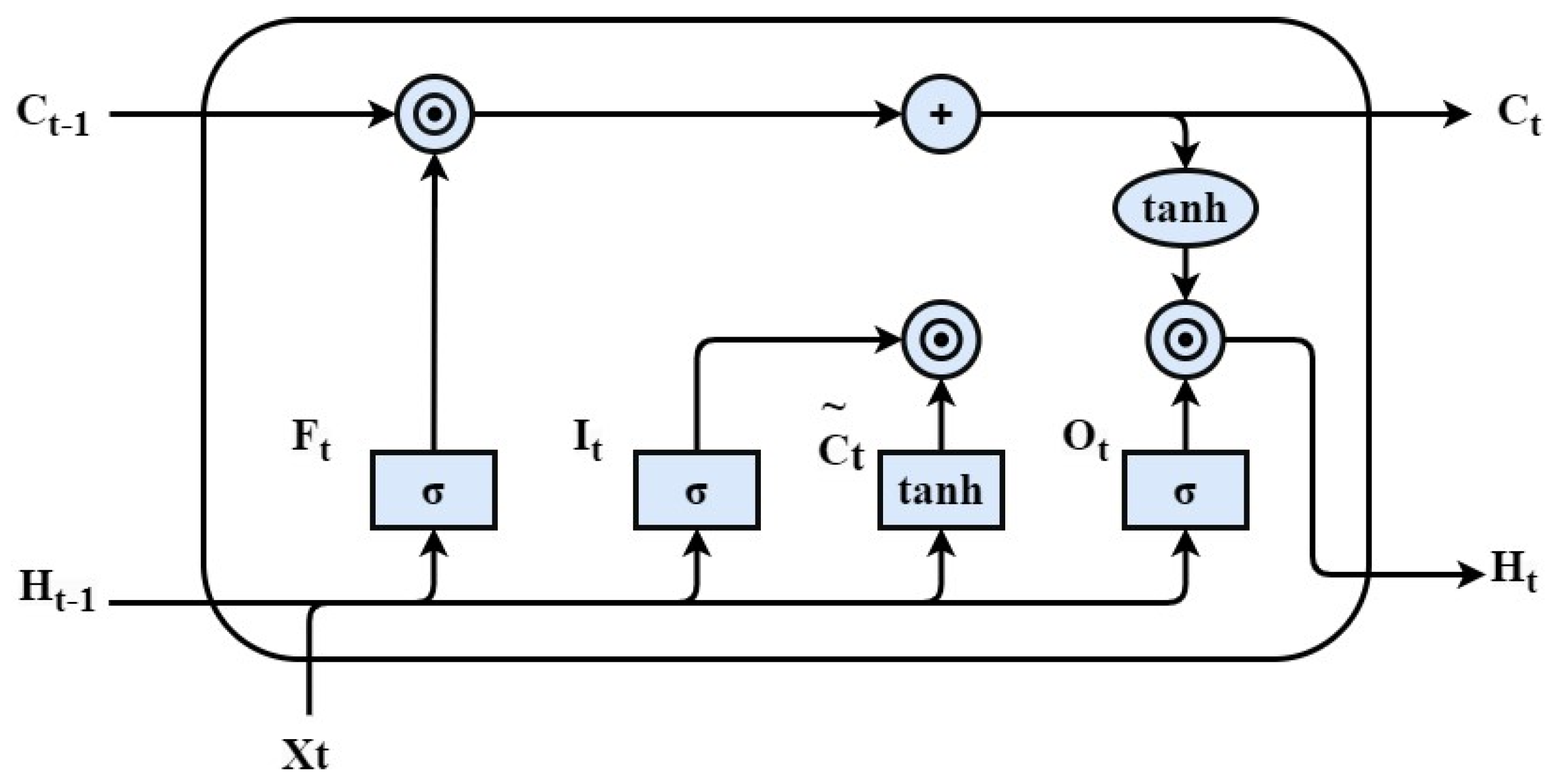
LSTM [26] networks were introduced to mitigate the challenge of vanishing gradients and effectively model long-term dependencies. LSTM represents a specialized variant of RNNs explicitly designed to tackle gradient instability encountered when training sequences with long time-series spans. By introducing more gating units to control the information flow within the network, the stability of the parameter optimization process is enhanced. The $Tanh$ function is used to extract valid information to alleviate the problem of vanishing gradients in the calculation of memory cells and hidden states. The LSTM architecture, depicted in Figure 3, incorporates memory cells and introduces several gating mechanisms to regulate the flow of information within the network. At each time step, the input $X_t$ from the current moment and the hidden state $H_{t-1}$ from the preceding moment are fed into the LSTM gates, which undergo processing via three fully connected layers equipped with sigmoid activation functions to compute the input, forget, and output gate values. This computation proceeds as follows:

$$\begin{array}{cc}\hfill I_t& =\sigma \left(X_t{W}_{xi}+H_{t-1}{W}_{hi}+b_i\right)\hfill \\ \hfill F_t& =\sigma \left(X_t{W}_{xf}+H_{t-1}{W}_{hf}+b_f\right)\hfill \\ \hfill O_t& =\sigma \left(X_t{W}_{xo}+H_{t-1}{W}_{ho}+b_o\right)\hfill \end{array}$$

(12)

where $W_{xc}$, $W_{xf}$, $W_{xo}$ and $W_{hi}$, $W_{hf}$, $W_{ho}$ are weight parameters and $b_i$, $b_f$, $b_o$ are bias parameters. The candidate memory element $\stackrel{\sim }{C_t}$ is calculated similarly to the gate but using the $tanh$ function as the activation function. Its equation at moment t is as follows:

$${\stackrel{\sim }{C}}_t=tanh\left(X_t{W}_{xc}+H_{t-1}{W}_{hc}+b_c\right)$$

(13)

where $W_{xc}$ and $W_{hc}$ are weight parameters and $b_c$ are bias parameters. Subsequently, the memory cells are computed, utilizing the previously derived input and forget gate values to determine the extent to which new data from candidate memory cells are incorporated while retaining relevant past information. This approach effectively mitigates the issue of vanishing gradients and facilitates capturing relationships with long-term dependencies within the time series. The computation of memory cells can be described as follows:

$$C_t=F_t\odot C_{t-1}+I_t\odot {\stackrel{\sim }{C}}_t$$

(14)

Figure 3. LSTM network structure.

Finally, the hidden state $H_t$ is computed, leveraging the output gate and memory cells. When the output gate is close to 1, it signifies the effective propagation of all memorized information to the prediction phase. Conversely, when the output gate is close to 0, it implies information retention solely within the memory cells without updating the hidden state. This computation unfolds as follows:

$$H_t=O_t\odot tanh\left(C_t\right)$$

(15)

LSTM has found extensive utility in natural language processing owing to its adeptness in handling long-term dependencies. The proposed model leverages LSTM to process time-series data, with the output of the LSTM layer serving as input to the subsequent attention mechanism layer, as elaborated upon in subsequent sections.

4.2. Self-Attention Mechanism

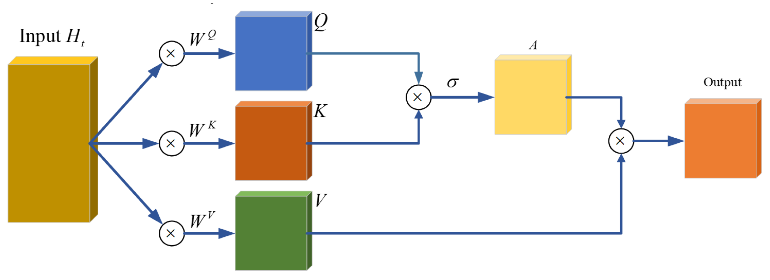
The Self-Attention mechanism represents a network configuration that comprehensively considers the overall context while prioritizing salient features. In time-series data, the information at any given moment is often interdependent on preceding moments. However, the correlation between data from different moments and the current moment varies. Therefore, during data training, incorporating information from previous moments and emphasizing the most pertinent information is crucial. This is commonly referred to as the Self-Attention mechanism.

The computational process of the Self-Attention mechanism is illustrated in Figure 4. The input $H_t$ is subjected to multiplication by three weight matrices $W^Q$, $W^K$, and $W^V$ to derive Q, K, and V, respectively. Subsequently, the resultant Q and K are used to compute the correlation between input vectors $\alpha$, typically through dot-multiplication. Normalization is then performed using the SoftMax function to obtain A. Finally, A is multiplied by V to yield the output of the Self-Attention mechanism layer.

Figure 4. Self-attentive machine architecture.

4.3. The Deep Learning Navigation Framework Based on Self-Attention

In the complex marine environment, the navigation and localization of AUVs predominantly rely on INS and DVL. However, DVL may produce invalid readings under certain conditions, such as encountering a school of fish, resulting in short-term data invalidation. Prolonged DVL invalidity occurs in ultra-deep waters or when encountering steep seabed slopes with no echo returns. While short-term invalidations can be compensated for using kinetic models, relying on such models for extended durations introduces deviations from actual velocities, impeding high-precision navigation and localization.

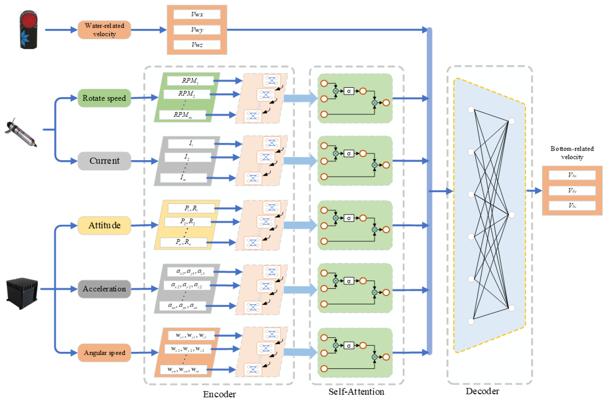
This section proposes a deep learning navigation framework based on the Self-Attention mechanism to achieve precise navigation over extended periods. The framework adopts an encoder–decoder architecture, organizing sensor data into time-series sequences inputted into the LSTM layer for encoding. Subsequently, time-series data are further refined through the Self-Attention mechanism, followed by decoding through fully connected layers and water-track velocity.

According to the AUV dynamics model outlined in Section 2, the velocity of the AUV correlates with acceleration, angular velocity, angle, thrust [27], and other factors. Acceleration encompasses triaxial acceleration in the instrument coordinate system, while angular velocity includes the triaxial angular velocity of the gyroscope. The angle comprises pitch and roll angles obtained from the INS. Thrust indirectly indicates the speed and current of twin thrusters. Although these data constitute time-series sequences, their sampling frequencies vary among sensors; for example, the collection frequency of the INS is 10, and the collection frequency of the thruster is 2. Although interpolation methods can be used to unify data of different frequencies to a common frequency, models built using this method may cause information increase and loss due to artificial data accumulation or interpolation. Separately processing data of different frequencies can also reduce the data preprocessing process. Additionally, separately processing data from different sources allows the encoder to only encode the data without handling the relationships between data, thus decoupling the network functionally and reducing repetitive work. Hence, data from sensors with different frequencies are inputted into corresponding LSTM layers. As depicted in Figure 5, this framework employs five LSTM layers to receive acceleration, angular velocity, angle, thruster speed, and current information. After extracting and compressing the time-series data of sensors into context vectors through the LSTM layer, the hidden layer serves as the input for further training on data significance at different moments through the Self-Attention mechanism layer. Finally, the Self-Attention mechanism layer output and the DVL-derived bottom-track velocity are fed into the fully connected layer for decoding.

Figure 5. Deep learning navigation framework.

The encoder–decoder architecture decouples the network, reducing redundancy while facilitating input–output sequence correspondence modeling. In the encoder stage, sensor time-series data are compressed into context vectors by LSTM, albeit with inevitable information loss. To address this information loss, a Self-Attention mechanism enhances time-series data encoding, learning correlations between input moments. The input in the decoder stage comprises timing vectors enhanced by the Self-Attention module. Given that the output solely represents the AUV velocity at the current moment without necessitating multiple sequence outputs, a linear layer is employed to map high-dimensional time-series vectors to a low-dimensional sample space, yielding the output of the model. To enhance model generalization during decoding, water-track velocity is encoded by LSTM and combined with timing input, serving as the final input to the linear layer. This enables the model to learn embedded sea current information.

The entire model can be summarized into two categories: First, LSTM and Self-Attention encode the timing information to obtain optimal timing vectors, addressing the long-term dependency problem and extending the inputs to high dimensions to extract effective information in all aspects. Second, the linear layer decoder maps the extracted time-series data to lower dimensions and learns the sea current information and water-track velocities to enhance the generalizability of the model and obtain the optimal output.

4.4. Portfolio Navigation Framework

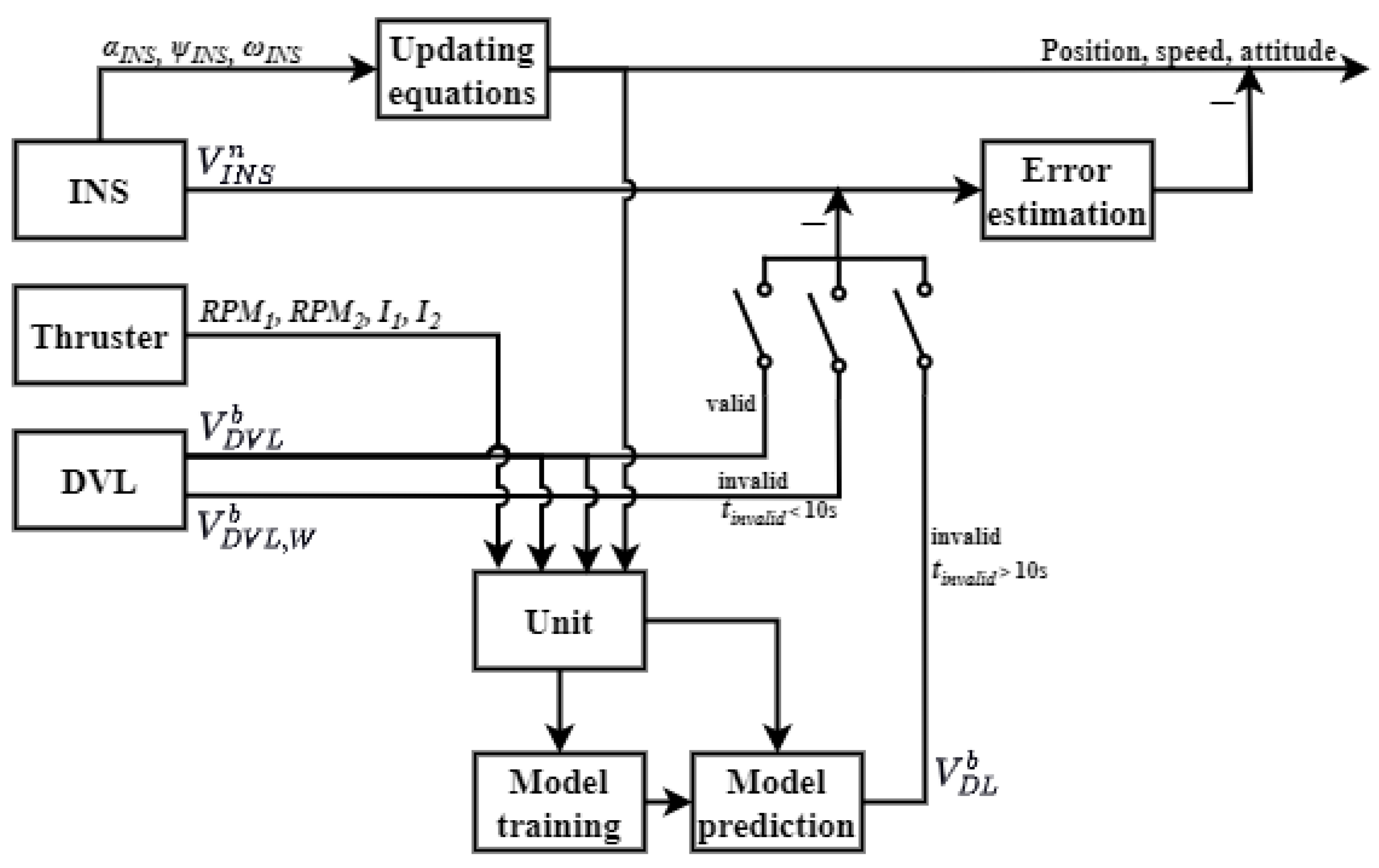
After constructing the deep learning navigation model based on Self-Attention as described in the previous subsection, the collected INS, DVL, and thruster data are divided into two paths when the DVL operates normally. One input feeds into the combined navigation model for AUV position computation, while the other input trains optimized network parameters for AUV speed estimation. During a short DVL failure, the Pathfinder DVL outputs a valid flag for the bottom-track velocity, where an A flag indicates that the measured bottom-track velocity is valid and any other flag indicates that it is invalid. Consequently, no more fault detection activity is performed, and the combination is navigated by compensating for the speed of the AUV using the water-track velocity. Conversely, during prolonged DVL invalidity, the DVL is determined to be invalid for a long time by calculating the time $t_{invalid}$ since the last valid flag bit. 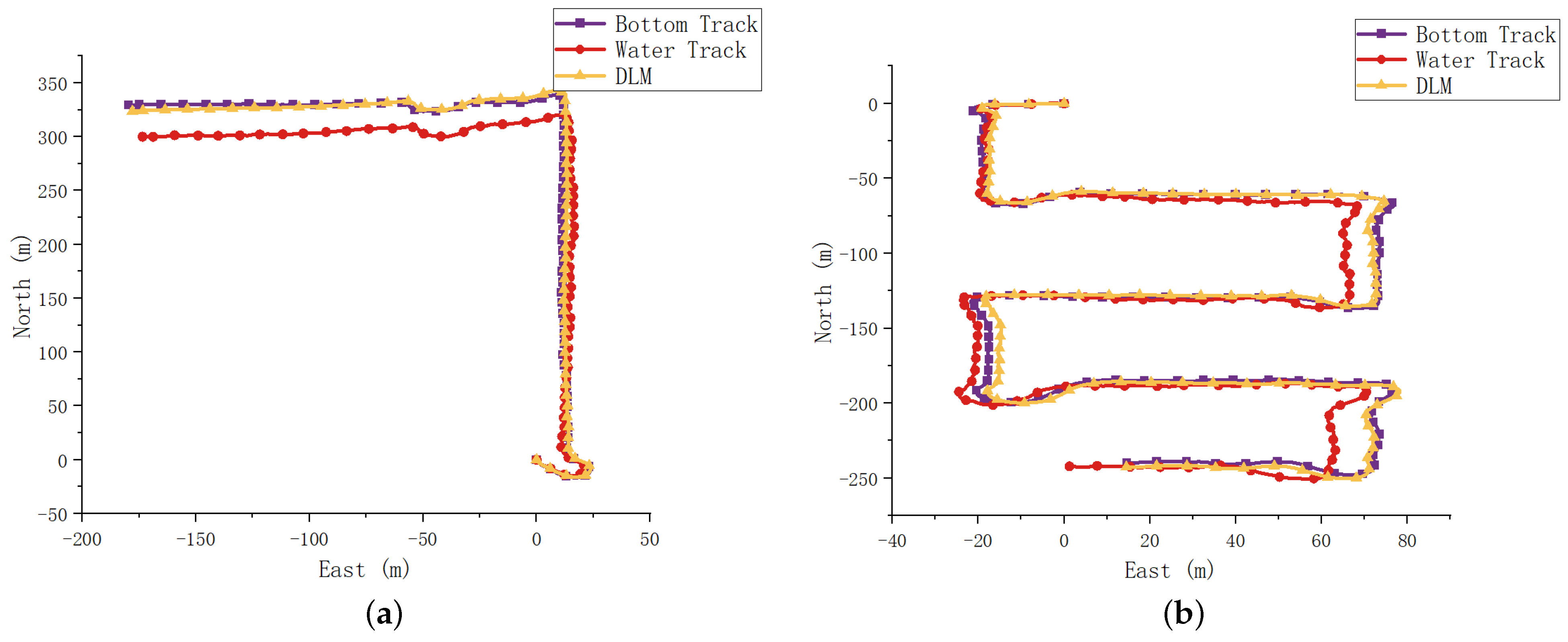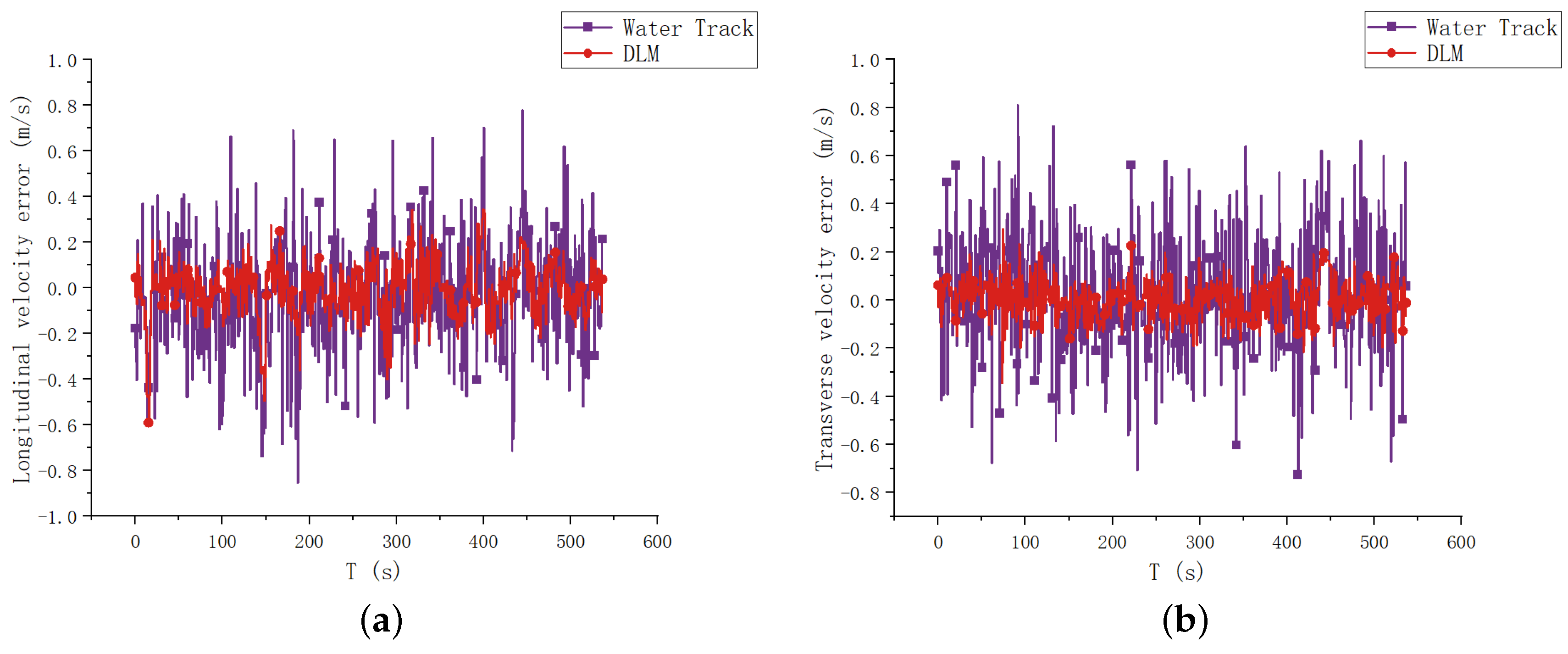When $t_{invalid}$ is larger than 10 s, the DVL for the bottom-velocity measurement is considered to have been invalid for a long time. At this point, the data from the corresponding sensors are fed into the AUV speed estimation model to predict the current AUV speed, and then the predicted speed is subtracted from the INS speed to obtain the measured value for optimal estimation. During the training and prediction of the AUV speed estimation model, the corresponding sensor data must be saved according to the set time interval. The frequency at which the DVL measures water-track velocity is used and is typically set to 1 s. The specific framework diagram is shown in Figure 6.

Figure 6. Combined navigation framework during DVL failure.

5. Experimental Results and Discussion

5.1. Test Configuration

To verify the performance of the proposed cruise speed estimation model, a large amount of data was collected at Xuejiadao Wharf, Qingdao, with the XH R300 AUV. The on-site experiment is shown in Figure 7. The data include acceleration, angular velocity, angle, water-track velocity, and bottom-track velocity at each acquisition moment. Additionally, rotational speed and current information are collected for the main thrusts. While bottom-track velocities serve as the target values for training, the remaining data are used as network input to predict velocity. After preprocessing the data, 19,010 pairs of data were selected as the training set and 3140 pairs of data as the validation set. The test set of Experiment 1 contains 4840 pairs of data and the test set of Experiment 2 contains 5340 pairs of data. And the deep learning framework was implemented using Pytorch, with model hyperparameters set as follows: the experiments were executed using NVIDIA GeForce GTX 1050Ti GPU; the time consumption on the training was about 20 ms; the number of nodes in the hidden layer of the LSTM and the output dimension of the Self-Attention layer were both set to 30; when Self-Attention was employed, its head was set to 2, indicating two parallel Self-Attention mechanism layers for extracting timing information from different aspects; the LSTM and Self-Attention dropout layers were set to 0; and the learning rate was set to 0.0001.

Figure 7. On-site experimental diagram.

5.2. AUV Real Experimental Data Test

GPS latitude and longitude were not selected as the ground truth values, as the deep-learning speed estimation model references bottom-track velocities. Instead, the trajectory derived from the bottom-track velocities was utilized. AUVs typically navigate in straight lines or execute comb trajectories based on mission requirements; hence, both scenarios were considered in experimental trajectory selection. Figure 8 illustrates a trajectory comparison between different methods, where purple represents trajectories computed using bottom-track velocities, red denotes trajectories computed using water-track velocities, and yellow depicts trajectories computed using velocities estimated by the Deep Learning Model (DLM). In Experiment 1 (Figure 8a), the trajectories exhibit minimal disparity during straight-line navigation. However, during turns, the trajectory derived from the water-track velocity lags, indicating diminished accuracy compared to the trajectory generated using the speed estimation model. Similar observations were noted in Experiment 2 (Figure 8b), particularly during comb trajectory execution.

Figure 8. Trajectory comparison chart. (a) Experiment 1, (b) Experiment 2.

Position error comparison in Figure 9 reveals consistent small errors in trajectories computed from speeds estimated by the deep learning model, irrespective of the experimental scenario. Conversely, trajectory errors computed from water-track velocity occasionally decrease but rapidly accumulate during maneuvers, resulting in noticeable divergence over time. The deep learning model effectively addresses this issue.

Figure 9. Position error comparison chart. (a) Experiment 1. (b) Experiment 2.

The estimated velocities of the bottom-track velocity, water-track velocity, and the speed estimation model are shown in Figure 10 and Figure 11, where the green lines are water-track velocities, the red lines are bottom-track velocities, and the blue lines are velocities estimated by the DLM. As can be seen in the figure, the water-track velocity has the largest amplitude, indicating that the measured velocity values are unstable. The reason for this is that the water-track velocity measures the velocity of the AUV relative to the water flow, which has a great deal of variability. However, the bottom-track velocity is more stable and has a smaller amplitude because it measures the velocity of the AUV relative to the seafloor, which is stationary. The velocities estimated by the DLM are as steady as the bottom-track velocity, and they have the same general trend. Consequently, the calculated trajectories are more consistent with those calculated for the bottom-track velocities.

Figure 10. Comparison of velocity for Experiment 1.

Figure 11. Comparison of velocity for Experiment 2.

Velocity error comparisons are presented in Figure 12 and Figure 13 for straight and comb trajectory cases, respectively, to further elucidate the problem. Fluctuations in the forward and rightward velocity errors are notably higher for the water-track velocity. This discrepancy arises from uncertainties in the water-mass flow velocity, impacting absolute velocity measurements. Conversely, the deep learning model incorporates water-track velocity, extracting flow information and mitigating error fluctuations. Table 4 lists the maximum and average value of forward speed errors, maximum and average value of rightward speed errors, and maximum and average value of position errors obtained from Experiments 1 and 2, indicating consistently smaller error parameters for the deep learning-based speed estimation model compared to the water-track velocity. Consequently, the speed estimation model can effectively improve the accuracy of navigation.

Figure 12. Comparison of velocity errors for Experiment 1. (a) Longitudinal velocity error. (b) Transverse velocity error.

Figure 13. Comparison of velocity errors for Experiment 2. (a) Longitudinal velocity error. (b) Transverse velocity error.

Table 4. Comparison chart of error parameters.

	Experiment 1       Experiment 2
	Water Track	DL	Water Track	DL
Maximum value of forward speed error (m/s)	0.853	0.266	0.853	0.591
Average of forward speed error (m/s)	0.192	0.067	0.201	0.088
Maximum value of rightward speed error (m/s)	1.030	0.320	0.810	0.345
Average of rightward speed error (m/s)	0.204	0.073	0.203	0.063
Maximum value of position error (m)	30.442	5.754	14.193	4.074
Average of position error (m)	12.420	2.784	5.889	1.973
Navigation accuracy	5.20%	0.90%	2.13%	0.48%

The experimental results on real data from the XH R300 demonstrate that the deep learning-based speed estimation model significantly enhances the combined navigation effectiveness of the DVL in cases of persistent bottom-track velocity failure. This study developed a deep learning speed estimation model based on LSTM and Self-Attention mechanisms, leveraging the time-series relationships among variables. Compensating the AUV velocity using the proposed model type was validated to incur less error compared to direct compensation with water-track velocity, thereby fulfilling the requirements of high-precision combined navigation. The cruise speed model did not consider large-scale vertical motions, which will be investigated in future work.

6. Conclusions

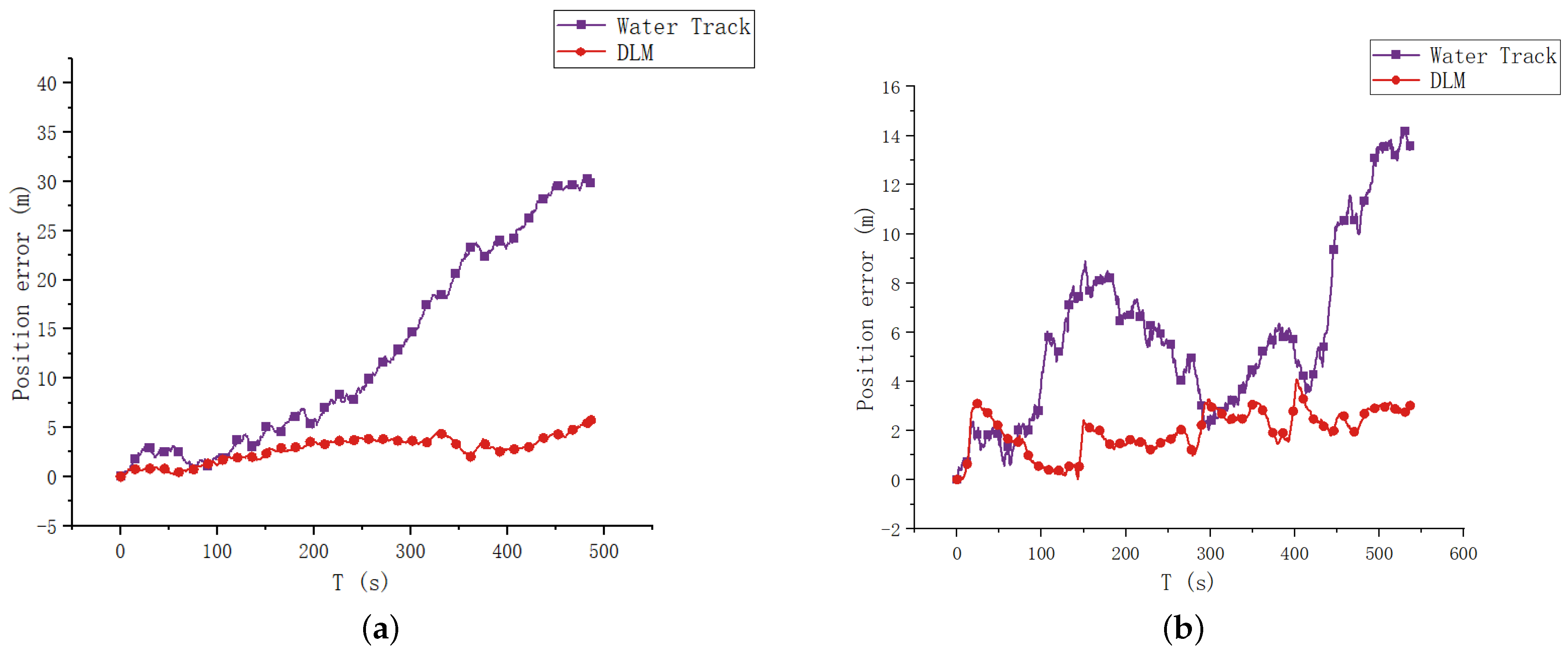
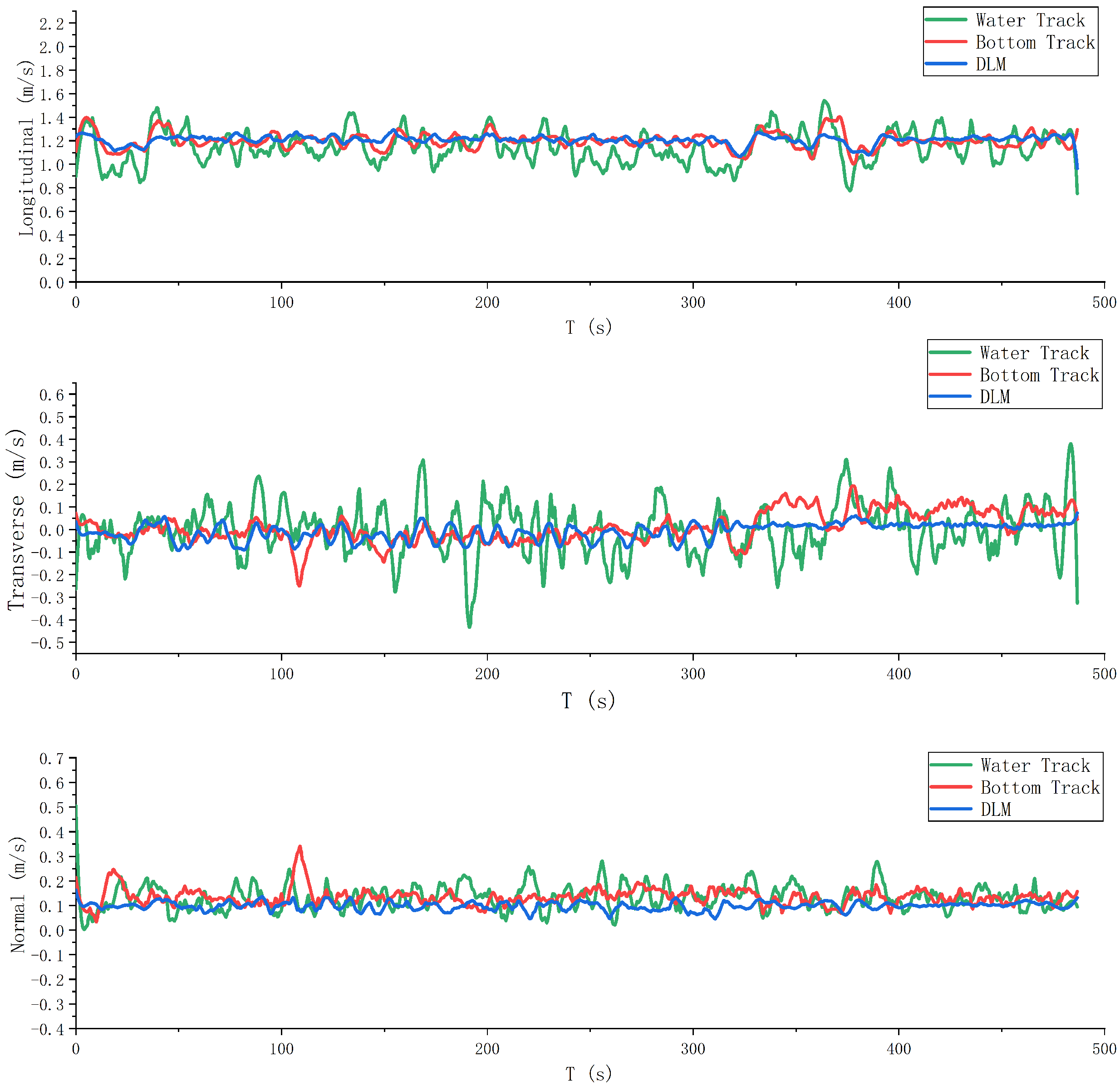
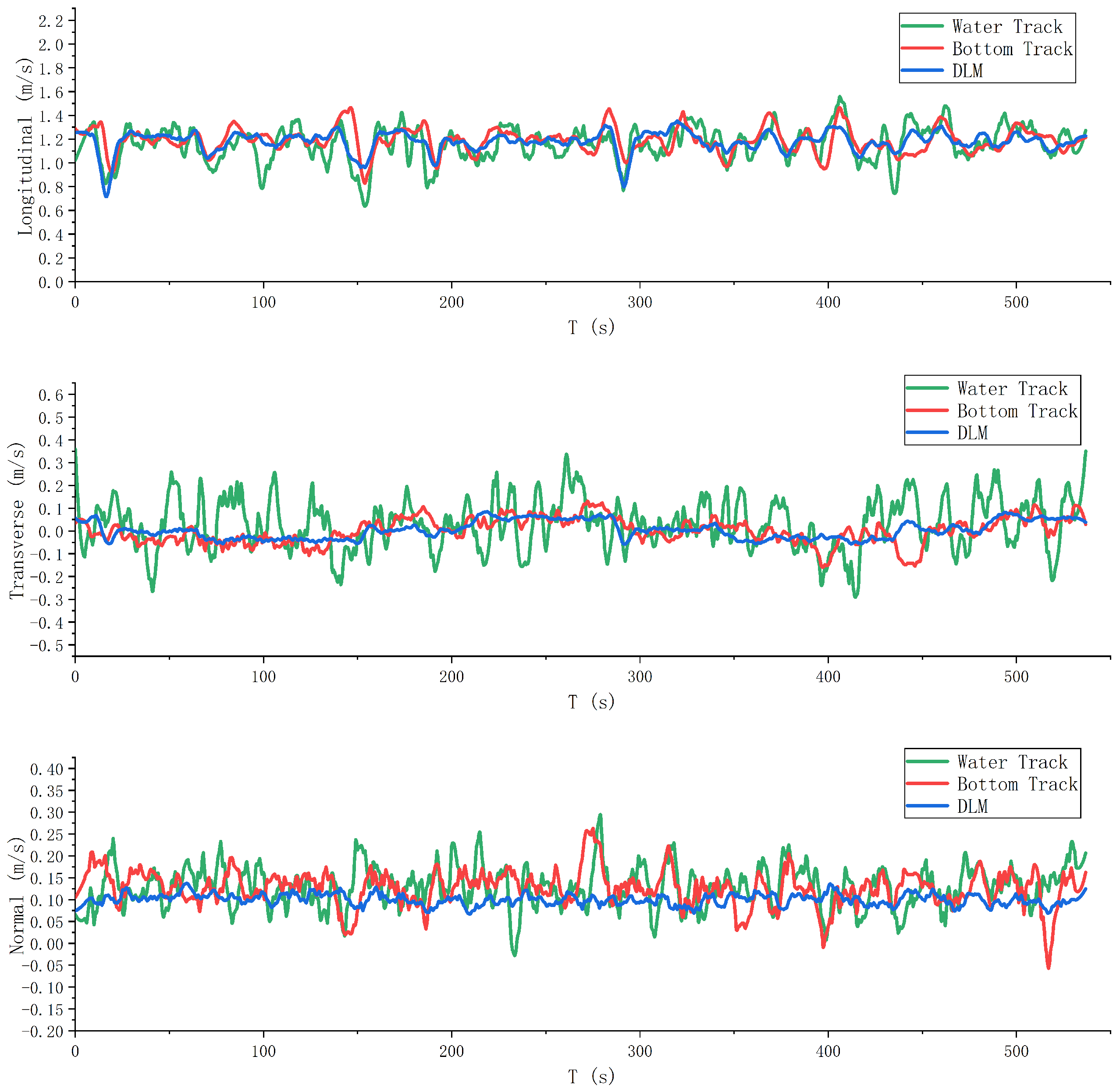
This study proposes a deep learning model leveraging acceleration, angle, angular velocity, and thruster speed as inputs to estimate AUV speed. LSTM is employed to extract time-series data from these variables, while Self-Attention enhances time-series data encoding to address long-term dependency issues. Water flow rate information, crucially embedded in water-track velocity, is separately encoded and utilized to enhance network generalization. The experimental results based on sea trial data demonstrate that the deep learning-based speed estimation model outperforms direct compensation with water-track velocity, achieving higher speed accuracy and meeting the demand for high-precision combined navigation in persistent DVL failure scenarios, thus enhancing the accuracy of the combined navigation system. Additionally, this research can be extended to scenarios with significant ocean currents, sharp turns, or muddy conditions that severely reduce DVL accuracy, further enhancing the reliability of the integrated navigation system.

Although the proposed method demonstrates superiority in most cases, the accuracy of the speed estimation model may deteriorate with declining bottom-track accuracy, warranting further investigation.