Communication

A Semi-Automatic Approach for Tree Crown Competition Indices Assessment from UAV LiDAR

1
CREA, Research Centre for Forestry and Wood, Viale Santa Margherita 80, IT-52100 Arezzo, Italy
2
Civil, Constructional and Environmental Engineering, Sapienza University, Piazzale Aldo Moro 5, IT-00185 Roma, Italy
*
Author to whom correspondence should be addressed.
Remote Sens. 2024, 16(14), 2576; https://doi.org/10.3390/rs16142576
Submission received: 7 June 2024 / Revised: 8 July 2024 / Accepted: 12 July 2024 / Published: 13 July 2024
(This article belongs to the Special Issue Novel Applications of UAV Imagery for Forest Science)

Abstract

:
Understanding the spatial heterogeneity of forest structure is crucial for comprehending ecosystem dynamics and promoting sustainable forest management. Unmanned aerial vehicle (UAV) LiDAR technology provides a promising method to capture detailed three-dimensional (3D) information about forest canopies, aiding in management and silvicultural practices. This study investigates the heterogeneity of forest structure in broadleaf forests using UAV LiDAR data, with a particular focus on tree crown features and their different information content compared to diameters. We explored a non-conventionally used method that emphasizes crown competition by employing a nearest neighbor selection technique based on metrics derived from UAV point cloud profiles at the tree level, rather than traditional DBH (diameter at breast height) spatial arrangement. About 300 vegetation elements within 10 plots collected in a managed Beech forest were used as reference data. We demonstrate that crown-based approaches, which are feasible with UAV LiDAR data at a reasonable cost and time, significantly enhances the understanding of forest heterogeneity, adding new information content for managers. Our findings underscore the utility of UAV LiDAR in characterizing the complexity and variability of forest structure at high resolution, offering valuable insights for carbon accounting and sustainable forest management.

1. Introduction

Light is among the major factors affecting tree growth, and tree crowns play a fundamental role in determining the amount of light and the microclimatic conditions experienced by all living organisms in forest ecosystems [1]. Crown size and shape influence various aspects of tree life, such as growth, mortality, stability, and reproductive success, consequently impacting the overall dynamics of the entire forest [2]. These features greatly depend on the spatial arrangement resulting from species-specific strategies, like lateral extension for light capture, maintenance of mechanical stability and hydraulic safety, and growth speed (i.e., slow versus fast growth) [3,4]. Besides these traits, forest management plays a central role. Predicting crown competition effects is crucial not only for ecological studies on natural forests but also for the economy of managed stands. A strong competition can indeed diminish the yield and vigor of single trees, potentially leading to their suppression and death.
Plenty of scientific literature grounds its results on simplified and geometric representations of crown features, appealing to our natural preference for schematization in understanding patterns and processes in nature [5]. However, numerous empirical studies indicate that variability in crown structure, rather than uniformity, is crucial for a tree’s success in dealing with competition [6]. Even in stands with a uniform canopy height, competition for canopy space and light tends to be asymmetric, contrasting with the quasi-symmetric behavior often assumed in forest studies. Partial shading from neighbors results in heterogeneous light distribution in the canopy. This leads to varied growth rates, with some sections experiencing slow growth and others exhibiting vigorous expansion. Trees exhibit plastic modifications to their canopy structure as a powerful response to these heterogeneous light conditions. They grow toward areas with higher light availability and reduced competition, thereby avoiding neighbors. Due to this morphological plasticity, tree canopies are rarely positioned directly above the stem base [7].
The so-called “neighborhood approach” is the basis of all studies that investigate small-scale tree-tree competition between trees of different sizes and/or different species [7,8]. Following this approach, (a) the identification of neighbors having an actual effect on the focal tree, and (b) a suitable selection of crown traits (for both k-neighbors and j-focal trees) are crucial steps. With some exceptions (e.g., Winkelmass, also known as uniform angle index, for which k is 4 [8,9,10]), spatial indices are very flexible in the number of neighbor trees.
The identification of neighbors with potential effects on the focal tree is usually based on the position of the DBH [10,11]. Nevertheless, the real tree-tree competition is at the root and crown level; the growth in DBH is only a reflection of how much plants accumulate in terms of water and light. Accurate measurement of tree crown features is therefore essential to better understand competition [7]. However, traditional methods for their precise measurement have limitations. Tools such as calipers (for diameters at breast height (DBH)), tapes (for crown projections) and, recently, a laser/sonar range finder (for total tree heights) are very time-consuming for 3D accurate measures and are subject to non-negligible positioning errors.
More recent is the use of terrestrial laser scanners (TLS, [12]). In that case, limitations arise in mature or even-aged forest stands, where the upper part of the canopy cannot be seen by the scanner, even in leaf-off conditions. Miniaturized, low-cost LiDAR instruments [13], mounted on UAV-LS and GPS-RTK systems to overcome these constraints. They enable precise co-registration of point clouds [14] and individual crown segmentation [15], reshaping the study of forest structure.
In the present study, we focused on evaluating the potential of UAV-LS to describe crown-crown features in a pure Beech-managed forest in Central Italy. Specific objectives are (1) present a new semi-automatic and dynamic method for effective tree-neighbor selection. (2) Obtain detailed crown projected area, and crown volume. (3) Evaluate the differences between the DBH differentiation index calculated using a fixed or dynamic number of neighbors and dimensional differentiation index [16] for the crown projected area, crown volume, and tree volume.
To do this, we used a set of Beech trees manually detected from co-registered TLS and UAV-LS data and analyzed following an approach recently introduced by ecologists on TLS data only [17]. TLS data, acquired simultaneously with UAV-LS, were used as a reference for tree stem positioning and traditional index calculations. We defined competitor—i.e., trees that are likely to impose competitive pressures on a focal tree—all those surrounding trees that were part of the upper canopy layer and were in direct contact with the crown of the focal tree (as for [7]).

2. Materials

This study was conducted in Alpe di Catenaia, Italy (Figure 1). The climate at the study site is temperate, with warm, dry summers and cold, rainy winters. The mean annual rainfall was 1224 mm, and the mean annual temperature was 9.5 °C. The monthly distribution of rainfall shows an autumn maximum in the month of November (165.1 mm) and a summer minimum in the month of July and a summer minimum in July (48.9 mm). Rainfall remains relatively high in the months of January to May (about 100 mm per month) and then decreases rapidly until the summer minimum. The average annual temperature is 9.2 °C, while the hottest month is July. The coldest month is January, followed by December and February. Beech even-aged forests, mainly aged between 70 and 90 years old, are prevalent in the study area [18]. Data were collected October–December 2023 over 10 circular sampling plots, 15 m radius of pure Beech forests characterized by arenaceous or marl-clay-sandstone substrata. Sampling plots were placed in the study area following a spatially balanced approach [19].
TLS-inventory measurements were performed by GeoSLAM ZEB-REVO (GeoSLAM Ltd., Ruddington, UK) lightweight mobile laser scanner. It features a rotating 2D scanning device and an inertial measurement unit in the handle. The system acquires 3D information about the surrounding area through measurements, due to the motion offered by the scanning head on the motor drive, enabling the application of 3D-simultaneous location and mapping algorithms [20]. This TLS requires that the starting and ending points of the scan process coincide, and some overlaps are carried out during the scan path. The center of the plot was georeferenced using a RTK GPS.
We collected UAV LiDAR (UAV-LS) data simultaneously with TLS measurements on the field. The UAV-LS LiDAR platform consisted of a DJI Matrice 350 quadcopter integrated with a Zenmuse L1 LiDAR sensor (DJI Inc., Shenzhen, China), an advanced scanning sensor designed for aerial surveying applications. It integrates a LiDAR module and an RGB camera with a non-full-frame configuration and an inertial measurement unit (IMU). It has a detection range of 450 m under 80% reflectivity conditions, a high point rate of up to 240,000 points per second, and ranging accuracy of 3 cm at a range of 100 m [21,22].
The flights were performed at approximately 55 m above the digital terrain model uploaded on UAV-LS, with approximately 13 km h−1 speed. With these settings, the resulting point cloud has a mean point density of about 1500 points m−2. Data processing was carried out in DJI Terra V4.1.0 software (DJI, Shenzhen, Guangdong, China) which allowed us to bring in the trajectory data of the drone flight, align the flight paths, georeference the point cloud, and then export it in LAS format.
Both TLS and UAV-LS data were collected during the leaf-off phenological phase. Every point cloud was clipped by corresponding 15 m radius circles and co-registered using CloudCompare software version 2.13 (Cloudcompare, Paris, France) following the procedure described in a previous work [14].

3. Methods

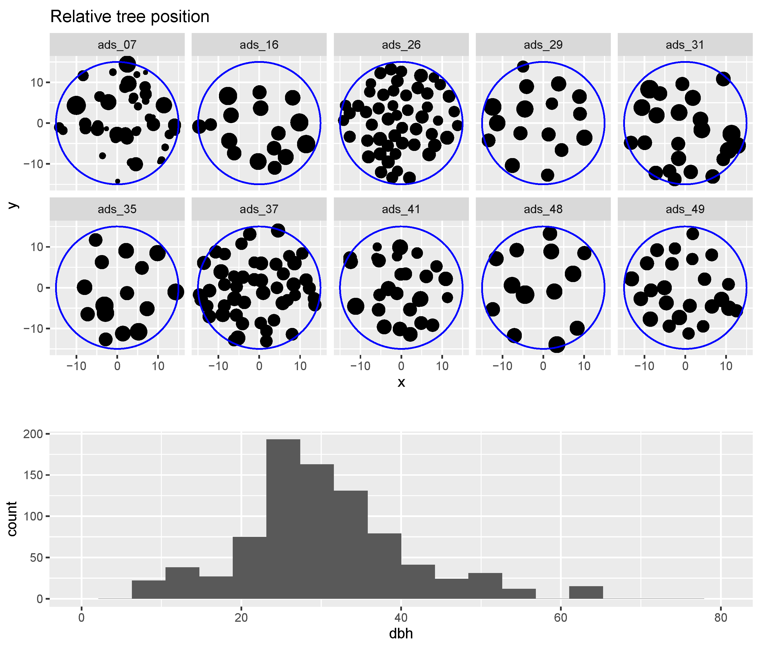
From the co-registered point cloud, we manually segmented a total of 299 trees (115 of which are focal trees). For each tree, we derived a tree XY-position and diameter at breast height (DBH, Figure 2), total tree height (TH), total tree volume (Tvol) and 3 crown features (see Section 3.1, Table 1).

3.1. Crown Features

Crown features were derived only from the UAV-LS component of co-registered point cloud. As crown features we computed: crown projected area (CrPrj), the XY-position of its centroid (xyCnt), and crown volume (CrVol). Using the lidR package (Roussel et al. [23]), we created a set of R algorithms that allowed to parameterize various structural crown attributes from the xyz-data of each focal tree and its neighbors. To do so, the single tree original point cloud (Figure 3, on the left) was first voxelized at a resolution of 25 cm (Figure 3), a good compromise for fast computation with mid-to-high-performance hardware. To avoid the residual noise in the original point cloud, only voxels with at least 3 points were considered “vegetation” and used to compute single tree vertical profiles. From its smoothed curve (red line in Figure 3), we derived the height of the maximum crown projection (Z peak, in meters), crown base height (Z peak start, in meters), and total tree height (Z peak end, in meters). Crown volume (CrVol) was computed as the sum of all vegetation voxels between Z peak start and Z peak end (Figure 3, dark-grey voxels in the center), while crown projected area (CrPrj) was calculated using a 2D convex hull (Figure 3, bottom-right).

3.2. Differentiation Dimensional Indices

Dimensional differentiation indices can be calculated by applying the following formula:
T X = 1 1 n k = 1 n m i n ( X i , X k ) m a x ( X i , X k )
were Xi and Xk are the tree-dimensional variable of interest for focal and surrounding trees, respectively [16]. For example, if we are interested in evaluating competition in diameter, following Equation (1), the DBH differentiation index [9] can be calculated as:
T 4 = 1 1 4 k = 1 4 m i n ( D B H i , D B H k ) m a x ( D B H i , D B H k )
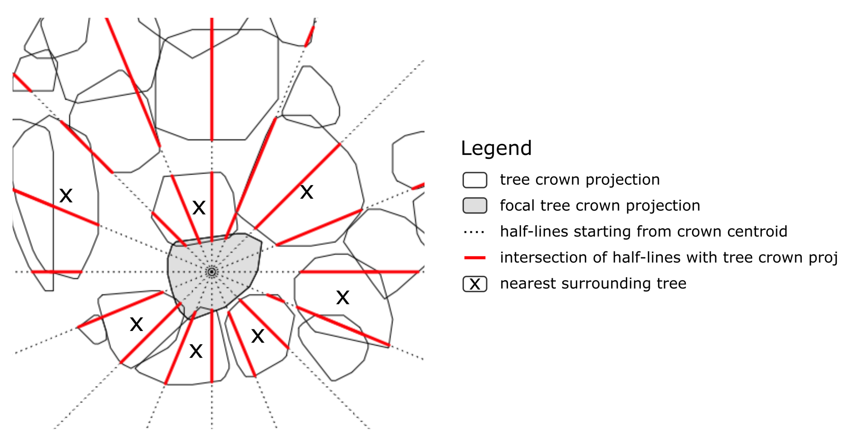
The number of nearest trees is usually a fixed number, frequently 4, i.e., the nearest trees in terms of DBH XY-position (Keren et al. [24]). Since tree-tree competition for light starts from the canopy, in this study we proposed a dynamic neighbor selection considering the crown position (Figure 4). In summary, starting from the crown centroid of the focal tree, we selected the nearest trees following an angular searching method, in order to detect the nearest trees from all directions. For details, see Figure 4’s caption. We then compared results between five different dimensional indices: (a) DBH differentiation index with k = 4 (T4, Equation (2)); (b) DBH differentiation index with variable number of nearest crowns (Td, Equation (3)); (c) crown projection differentiation index (TCrPrj, Equation (4)); (d) crown volume differentiation index (TCrVol, Equation (5)); (e) tree volume differentiation index (Tvol, Equation (6)).
T d = 1 1 n k = 1 n m i n ( D B H i , D B H k ) m a x ( D B H i , D B H k )
T C r P r j = 1 1 n k = 1 n m i n ( C r P r j i , C r P r j k ) m a x ( C r P r j i , C r P r j k )
T C r V o l = 1 1 n k = 1 n m i n ( C r V o l i , C r V o l k ) m a x ( C r V o l i , C r V o l k )
T v o l = 1 1 n k = 1 n m i n ( v o l i , v o l k ) m a x ( v o l i , v o l k )

3.3. Statistical Analysis

We tested all calculated indices for normality with the Shapiro–Wilk test. Where indices exhibited non-normal frequency distributions and/or heteroscedasticity, multiple paired Wilcoxon tests were conducted to determine the index values that differed significantly. All statistical tests were conducted at α = 0.05. Data analysis was performed in the R statistical package, Version 4.2.3 (Team [25]).

4. Results

4.1. Single Tree Manual Segmentation

We first tried with automatic segmentation methods, using already developed methods and tools (e.g., Treeiso, a function built on CloudCompare software version 2.13 (Cloudcompare, Paris, France)), but results were not satisfactory: a lot of sparse clusters in the canopy layer were associated with the wrong tree. Then we opted for a manual method on Trimble RealWorks (Figure 3). The time required to create the reference dataset depends, as expected, on the complexity of the forest stand and stand density. Since we measured trees from even-aged populations with similar top heights and crowns occupying the same forest layer, the greatest obstacle to segmentation was branches intertwining. In total, 18 person-days were needed to isolate and measure the Beech trees from which the 115 focal trees and their respective neighbors were selected, with an average of 1.8 days per sampling plot. The duration of this phase mainly depends on the size of the trees.

4.2. Tree-Neighbors Selection

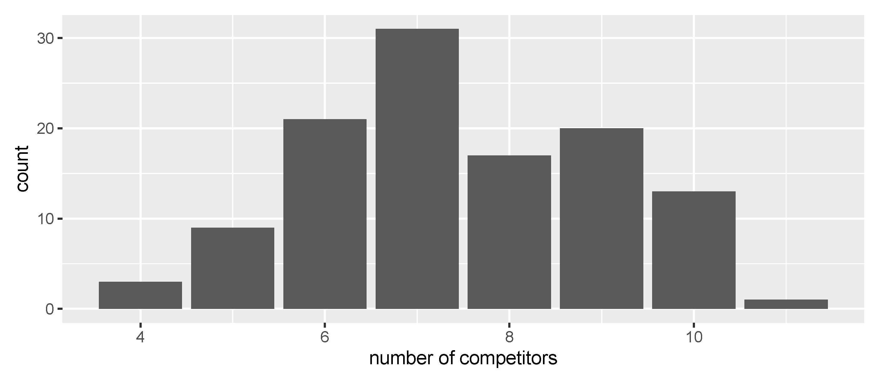
Using the method described in Section 3 and Figure 4, the average number of competitors is 7.45, with a standard deviation of 1.60, the median is 7. A focal tree is surrounded by 4 competitors (lowest value) in just 3 cases over 115, and by 10 or 11 competitors (highest values) in 14 cases (Figure 5).

4.3. Crown Projected Area and Crown Volume

From the results, CrPrj and CrVol are highly correlated (Pearson correlation coefficient, r = 0.96). In even-aged forests, the mean crown projection area (CrPrj) at tree level is inversely proportional to tree density. In this study, the maximum CrPrj (33.9 m2) was reached in ads_34, where the density is the lower (127.3 trees ha−1, Table 2). On the other side, ads_37 and ads_26, with respectively 679.1 and 735.6 trees ha−1 (i.e., the highest densities), have the lowest CrPrj values (8.2 and 7.8 m2, respectively).
Also, mean CrVol at plot level decrease when tree density increases (Table 2). Despite this general behavior, plots with similar densities (e.g., ads_29 and ads_35) have really different crown volumes (respectively 79 and 54 m3), unveiling a certain variability also for those apparently similar forest structure.

4.4. Indices Statistic Analysis

All the indices exhibited non-normal frequency distribution. Table 3 shows the two-sample Wilcoxon test results (with Bonferroni correction for multiple comparisons).
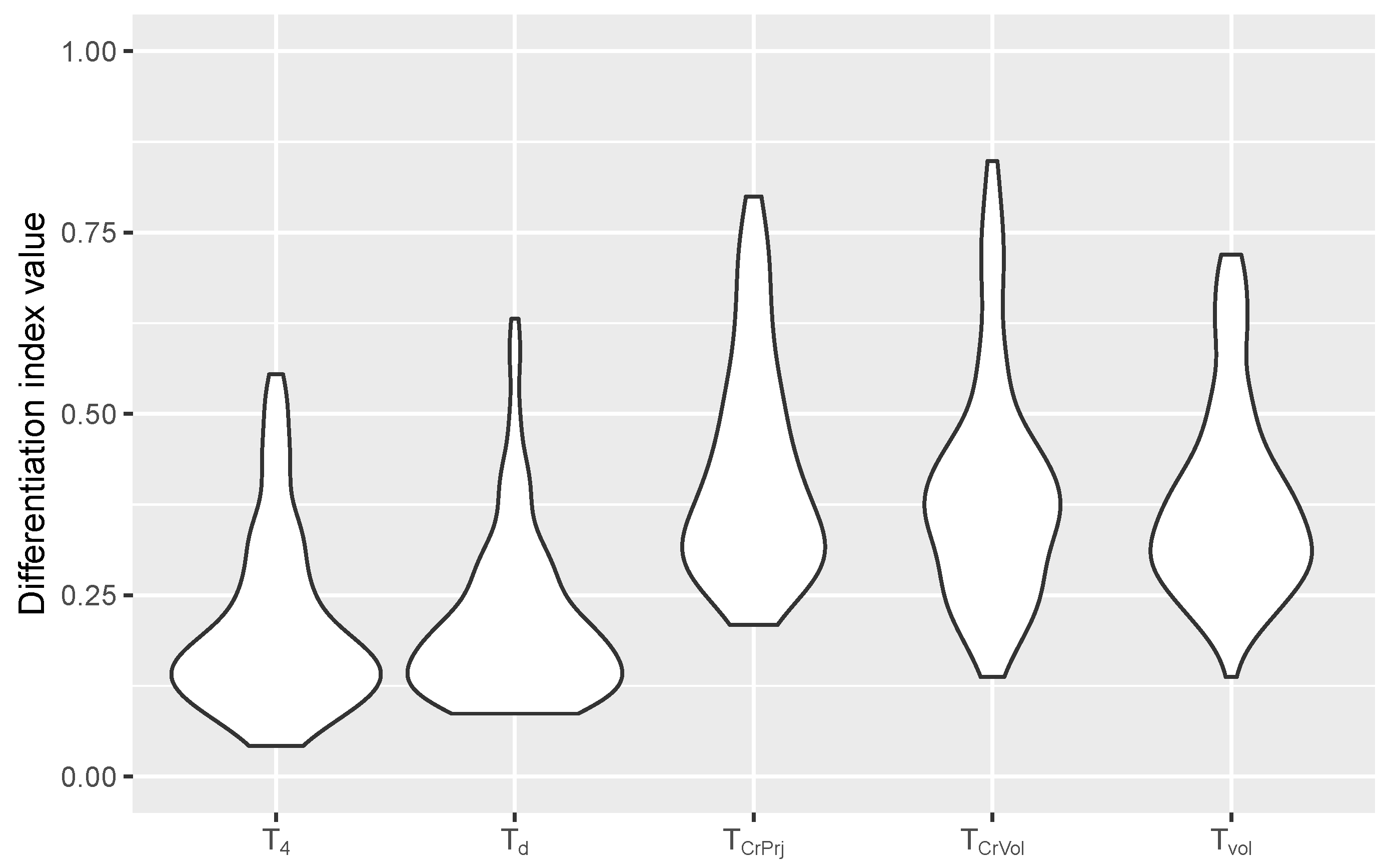
The statistical analysis showed that the index based on DBH, calculated using a dynamic number of neighbors (Td, mean = 0.21; sd = 0.11), yielded almost the same index values as when four neighbor DBH were used (T4, mean = 0.20; sd = 0.12), although the DBH differentiation index based on four neighbors (T4) has slightly lower values than Td (Figure 6). This result was confirmed by the two-sample Wilcoxon test applied to T4 and Td distributions (p-value = 1, Table 3).
Both mean values (0.38) and standard deviation (0.13) for Tvol are similar to—but slightly lower than—TCrPrj (mean = 0.42; sd = 0.15) and TCrVol (mean = 0.40; sd = 0.16). Following Wilcoxon test results from Table 3, they significantly differ from T4, and Td p-value is always lower than 0.001 for all the pairs). Moreover, Tvol and TCrPrj showed a significant difference in distribution (p-value = 1.69 × 10⁻⁴).

5. Discussion

Incorporating different crown traits in spatial index computation allows to obtain results with varying levels of informational content, offering diverse perspectives on stand complexity. Tree structural characteristics cannot be fully captured by diameter measurements alone or by quick canopy surveys from the ground [26]. Specifically, using parameters such as diameter, tree volume, and the apparent volume of the canopy in the calculation of diversity indices reveals different levels of heterogeneity. This variance is reflected not only in the average values and their variability, but also in the entire distribution of values. By examining these different characteristics, a more comprehensive understanding of the structural diversity within the forest stand can be derived, highlighting the multifaceted nature of its complexity.
If compared with airborne laser scanning, the higher scanning density guaranteed by UAV-LS data allows for more detailed measurement of crown features and spatial arrangement of trees, even in homogeneous stands like those analyzed in this study. Employing UAV-LS for tree level analysis not only improves the accuracy of measurements but also enhances the ability to monitor and study the growth patterns and structural changes in larger, older trees. An additional advantage offered by both TLS and UAV-LS point clouds relies on the accurate measure of large trees, which are often more challenging to measure using analog or traditional methods such as calipers and vertex hypsometers.
In this paper, a general workflow for spatial index computation from UAV-LS point clouds were developed and presented. With well segmented single trees, the automatic step for delineating crown projection, and computing crown volume works fast (about 1 s for each tree) and without computational bottlenecks. However, removing the noise from the point clouds and manually isolating trees require time, specialized digital skills, and advanced data processing techniques. Still today, automatic segmentation is a challenging task, especially in broadleaf forests where branches intertwine extensively. All current automatic methods require some level of visual or manual verification to ensure accuracy.
Compared with previous studies [7], where 15 trees (Ash, Beech and Hornbeam) were measured by TLS, UAV-LS technology, which can survey hectares in a few minutes, allowing us to consistently increase the number of focal trees to 115. Our results are in line with those from other similar studies [24,27,28]. In particular, in even-aged Beech forests with a simplified structure, like the ones we analyzed, an adequate number of competitors seems to be 7 or 8, a considerably higher value if compared with the traditional number of nearest neighbors (i.e., k = 4). Further, the real potential of the proposed methodology relies on the high adaptability in identifying the best number of competitors at tree level.
Despite this, the comforting results obtained in this experiment cannot be directly extended to all the different forest structures characterizing Beech forests, mixed forests, or other forest types. Future research should aim to apply this methodology to diverse forest ecosystems to validate its effectiveness across different conditions.

6. Conclusions

Our study demonstrates the significant advantages of UAV-LS technology in forest monitoring and management. UAV-LS provides detailed and extensive coverage of tree crown features and spatial arrangements, offering an efficient alternative to traditional ground-based approaches. This technology saves time and resources while enhancing the accuracy and detail of forest stand analysis.
Being focused on pure Beech stands, this paper has a limited replicability both in other forest types and in mixed stands. Nonetheless, Beech forest has a pan-European range of distribution, so this approach has a definitively large area of application. Moreover, we highlighted the value of these studies in understanding pure Beech stand competition dynamics and structural complexities. Our findings align with previous research, confirming that the choice of neighbor tree selection methods does not significantly affect structural indices. However, incorporating crown traits into heterogeneity indices provides diverse and significant insights into forest complexity, underscoring the multifaceted nature of forest structure.
In summary, UAV-LS technology offers substantial benefits for forest management and silviculture. It enhances the efficiency and effectiveness of management practices, supports accurate predictions, and modeling, and facilitates better decision-making. This holistic approach ensures sustainable management of forest resources, taking into account both ecological dynamics and economic viability.

Author Contributions

N.P.: Conceptualization, Project administration, Supervision, Methodology, Formal analysis, Writing—review and editing; M.G.: Data collection; S.I.: Data collection; L.C.: Methodology, Formal analysis, Writing—review and editing; U.C.: Conceptualization, Supervision, Methodology, Writing—review and editing. All authors have read and agreed to the published version of the manuscript.

Funding

This research was funded with the contribution of the Italian Ministry of Agricultural, Food, and Forestry Policies (MiPAAF) sub-project “Precision Forestry” (AgriDigit program) (DM 36503.7305.2018 of 20 December 2018).

Informed Consent Statement

Informed consent was obtained from all subjects involved in the study.

Data Availability Statement

Data presented in this study are available at the links mentioned in the text or on request from the corresponding author.

Conflicts of Interest

The authors declare no conflict of interest.

References

  1. Dial, R.; Bloodworth, B.; Lee, A.; Boyne, P.; Heys, J. The Distribution of Free Space and Its Relation to Canopy Composition at Six Forest Sites. For. Sci. 2004, 50, 312–325. [Google Scholar] [CrossRef]
  2. Hildebrand, M.; Perles-Garcia, M.D.; Kunz, M.; Härdtle, W.; Von Oheimb, G.; Fichtner, A. Tree-tree interactions and crown complementarity: The role of functional diversity and branch traits for canopy packing. Basic Appl. Ecol. 2021, 50, 217–227. [Google Scholar] [CrossRef]
  3. Verkerk, P.J.; Fitzgerald, J.B.; Datta, P.; Dees, M.; Hengeveld, G.M.; Lindner, M.; Zudin, S. Spatial distribution of the potential forest biomass availability in Europe. For. Ecosyst. 2019, 6, 5. [Google Scholar] [CrossRef]
  4. Aalto, I.; Aalto, J.; Hancock, S.; Valkonen, S.; Maeda, E.E. Quantifying the impact of management on the three-dimensional structure of boreal forests. For. Ecol. Manag. 2023, 535, 120885. [Google Scholar] [CrossRef]
  5. Pretzsch, H.; Dieler, J. Evidence of variant intra- and interspecific scaling of tree crown structure and relevance for allometric theory. Oecologia 2012, 169, 637–649. [Google Scholar] [CrossRef]
  6. Pretzsch, H. The Effect of Tree Crown Allometry on Community Dynamics in Mixed-Species Stands versus Monocultures. A Review and Perspectives for Modeling and Silvicultural Regulation. Forests 2019, 10, 810. [Google Scholar] [CrossRef]
  7. Seidel, D.; Leuschner, C.; Müller, A.; Krause, B. Crown plasticity in mixed forests—Quantifying asymmetry as a measure of competition using terrestrial laser scanning. For. Ecol. Manag. 2011, 261, 2123–2132. [Google Scholar] [CrossRef]
  8. Hui, G.; Gadow, K. Das Winkelmass—Herleitung des optimalen Standardwinkels. Allg. Forst Jagdztg. 2002, 173, 173–176. [Google Scholar]
  9. Pommerening, A. Evaluating structural indices by reversing forest structural analysis. For. Ecol. Manag. 2006, 224, 266–277. [Google Scholar] [CrossRef]
  10. Zhang, M.; Wang, J.; Kang, X. Spatial distribution pattern of dominant tree species in different disturbance plots in the Changbai Mountain. Sci. Rep. 2022, 12, 14161. [Google Scholar] [CrossRef]
  11. Pommerening, A.; Wang, H.; Zhao, Z. Global woodland structure from local interactions: New nearest-neighbour functions for understanding the ontogenesis of global forest structure. For. Ecosyst. 2020, 7, 22. [Google Scholar] [CrossRef]
  12. Disney, M. Terrestrial LiDAR: A three-dimensional revolution in how we look at trees. New Phytol. 2019, 222, 1736–1741. [Google Scholar] [CrossRef] [PubMed]
  13. Torresan, C.; Berton, A.; Carotenuto, F.; Chiavetta, U.; Miglietta, F.; Zaldei, A.; Gioli, B. Development and Performance Assessment of a Low-Cost UAV Laser Scanner System (LasUAV). Remote Sens. 2018, 10, 1094. [Google Scholar] [CrossRef]
  14. Puletti, N.; Innocenti, S.; Guasti, M. A co-registration approach between terrestrial and UAV laser scanning point clouds based on ground and trees features. Ann. Silvic. Res. 2024, 49, 4466. [Google Scholar] [CrossRef]
  15. Torresan, C.; Pelleri, F.; Manetti, M.; Becagli, C.; Castaldi, C.; Notarangelo, M.; Chiavetta, U. Comparison of TLS against traditional surveying method for stem taper modelling. A case study in European beech (Fagus sylvatica L.) forests of mount Amiata. Ann. Silvic. Res. 2021, 46, 128–140. [Google Scholar]
  16. Szmyt, J.; Korzeniewicz, R. Do natural processes at the juvenile stage of stand development differentiate the spatial structure of trees in artificially established forest stands? For. Res. Pap. 2014, 75, 171–179. [Google Scholar] [CrossRef]
  17. Owen, H.J.F.; Flynn, W.R.M.; Lines, E.R. Competitive drivers of interspecific deviations of crown morphology from theoretical predictions measured with Terrestrial Laser Scanning. J. Ecol. 2021, 109, 2612–2628. [Google Scholar] [CrossRef]
  18. Cutini, A.; Chianucci, F.; Giannini, T.; Manetti, M.C.; Salvati, L. Is anticipated seed cutting an effective option to accelerate transition to high forest in European beech (Fagus sylvatica L.) coppice stands? Ann. For. Sci. 2015, 72, 631–640. [Google Scholar] [CrossRef]
  19. Fattorini, L.; Puletti, N.; Chirici, G.; Corona, P.; Gazzarri, C.; Mura, M.; Marchetti, M. Checking the performance of point and plot sampling on aerial photoimagery of a large-scale population of trees outside forests. Can. J. For. Res. 2016, 46, 1264–1274. [Google Scholar] [CrossRef]
  20. Puletti, N.; Grotti, M.; Ferrara, C.; Chianucci, F. Lidar-based estimates of aboveground biomass through ground, aerial, and satellite observation: A case study in a Mediterranean forest. J. Appl. Remote. Sens. 2020, 14, 044501. [Google Scholar] [CrossRef]
  21. Diara, F.; Roggero, M. Quality Assessment of DJI Zenmuse L1 and P1 LiDAR and Photogrammetric Systems: Metric and Statistics Analysis with the Integration of Trimble SX10 Data. Geomatics 2022, 2, 254–281. [Google Scholar] [CrossRef]
  22. Štroner, M.; Urban, R.; Línková, L. A New Method for UAV Lidar Precision Testing Used for the Evaluation of an Affordable DJI ZENMUSE L1 Scanner. Remote. Sens. 2021, 13, 4811. [Google Scholar] [CrossRef]
  23. Roussel, J.R.; Auty, D.; Coops, N.C.; Tompalski, P.; Goodbody, T.R.; Meador, A.; Bourdon, J.; De Boissieu, F.; Achim, A. lidR: An R package for analysis of Airborne Laser Scanning (ALS) data. Remote. Sens. Environ. 2020, 251, 112061. [Google Scholar] [CrossRef]
  24. Keren, S.; Svoboda, M.; Janda, P.; Nagel, T.A. Relationships between Structural Indices and Conventional Stand Attributes in an Old-Growth Forest in Southeast Europe. Forests 2019, 11, 4. [Google Scholar] [CrossRef]
  25. Team, R.C. R: A Language and Environment for Statistical Computing; R Foundation for Statistical Computing: Vienna, Austria, 2023. [Google Scholar]
  26. Juchheim, J.; Ammer, C.; Schall, P.; Seidel, D. Canopy space filling rather than conventional measures of structural diversity explains productivity of beech stands. For. Ecol. Manag. 2017, 395, 19–26. [Google Scholar] [CrossRef]
  27. Keren, S.; Diaci, J.; Motta, R.; Govedar, Z. Stand structural complexity of mixed old-growth and adjacent selection forests in the Dinaric Mountains of Bosnia and Herzegovina. For. Ecol. Manag. 2017, 400, 531–541. [Google Scholar] [CrossRef]
  28. Parobeková, Z.; Pittner, J.; Kucbel, S.; Saniga, M.; Filípek, M.; Sedmáková, D.; Vencurik, J.; Jaloviar, P. Structural Diversity in a Mixed Spruce-Fir-Beech Old-Growth Forest Remnant of the Western Carpathians. Forests 2017, 2018, 379. [Google Scholar] [CrossRef]
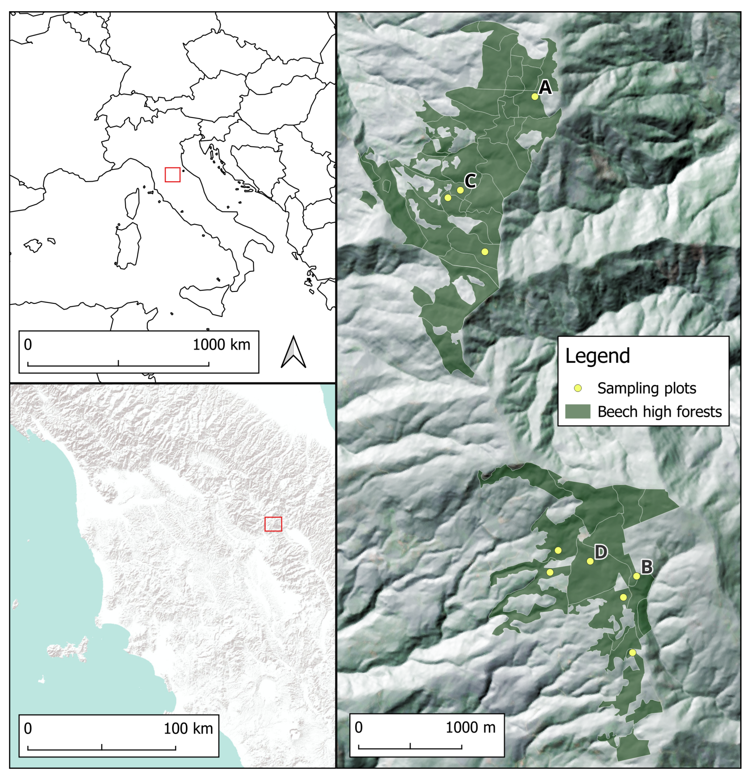
Figure 1. Study area, Beech forested area (green), and sampling plot location (yellow points). Esri Terrain and Regional DTM were used as bases for the figures on the left and on the right, respectively.
Remotesensing 16 02576 g001
Figure 2. On the top: Tree positions for sampling plots considered in this study. Point size is proportional to DBH. Below: histogram of DBH distribution for trees measured.
Remotesensing 16 02576 g002
Figure 3. Workflow of the entire process from original point cloud of sampling plot (top-right) to manual segmentation of each tree in the plot. On the bottom: the three-dimensional point cloud of a single tree (left) was voxelized (center). Red-line on the right is the smoothed vertical profile of the same tree. Convex hull polygon of crown projection at the ‘Z peak’ height for a single tree and for an entire plot (bottom-right).
Remotesensing 16 02576 g003
Figure 4. Proposed neighbors’ selection for a focal tree (in gray). Starting from crown centroid, the algorithm sketches 16 half-lines dividing the round angle into 16 equal angles 22.5° each. A neighbor crown is selected if one of 16 half-lines intersect it (red lines). As final step, only nearest intersected crowns in the same half-line were selected as neighbor trees (marked with a “X” in the figure).
Remotesensing 16 02576 g004
Figure 5. Frequency distribution of the number of surrounding competitors for the 115 focal trees analyzed in this study.
Remotesensing 16 02576 g005
Figure 6. Violin plot of index value distribution. From left: DBH differentiation index with k = 4 ( T 4 ); DBH differentiation index with k nearest crowns ( T d ); crown projection differentiation index ( T C r P r j ); crown volume differentiation index ( T C r V o l ); tree volume differentiation index ( T v o l ).
Remotesensing 16 02576 g006
Table 1. Descriptive parameters at plot level: mean and standard deviations (in brachets) for diameter at breast height ( D B H , cm ), total tree height ( T H , m), tree wood volume ( v o l , m 3 ) of trees. All the sampling plots belong to pure Beech forest stands, with same climatic conditions. All UAV LiDAR and field data were collected during winter 2023 (leaf-off phenological phase).
ads idN ha−1DBHTHvol
ads_07679.121.6 (13.4)23.9 (3.8)0.7 (0.9)
ads_16226.444 (10.9)23.1 (1.4)1.7 (1)
ads_26735.625.4 (3.8)15.4 (1.9)0.3 (0.1)
ads_29226.438.4 (9.3)21.5 (1.8)1.5 (0.8)
ads_31325.442.8 (9.3)21.8 (1.6)1 (0.5)
ads_34127.348.9 (21.5)23.1 (1.3)1.9 (1.5)
ads_35212.243.3 (9.7)25.1 (1.4)1.4 (0.6)
ads_37679.130.2 (4.2)22.4 (1.7)0.7 (0.2)
ads_41382.032.1 (8.7)21.1 (1.7)1 (0.8)
ads_48183.944.3 (8.5)27.5 (1)2.3 (0.8)
ads_49339.533.6 (5.7)25.3 (1.3)0.9 (0.3)
Total411.732.5 (12.2)21.8 (4)0.9 (0.8)
Table 2. Crown features (plot level results): mean and standard deviations (in brachets) for crown projection area ( C r P r j , m 2 ) and crown volume ( C r V o l , m 3 ) of trees.
ads idN ha−1CrPrjCrVol
ads_07679.110.3 (13.6)26.1 (34.2)
ads_16226.427.9 (19.9)79.4 (55.1)
ads_26735.67.8 (4.2)17.9 (8.2)
ads_29226.428.8 (15.1)79.6 (47)
ads_31325.421.9 (13.2)53.3 (31.3)
ads_34127.333.9 (22)85.9 (49.6)
ads_35212.225.4 (9.9)53.9 (29.6)
ads_37679.18.2 (4.2)22.8 (10.1)
ads_41382.015.3 (13)39.8 (33.9)
ads_48183.927.9 (11.2)92.1 (37.7)
ads_49339.515.6 (6.3)35 (13.6)
Total411.715.6 (13.8)40.4 (37.5)
Table 3. p-values of the two-sample Wilcoxon test (with Bonferroni correction for multiple comparisons) for all possible pairs among the considered indices.
T d T 4 T CrPrj T CrVol
T 4 1
T C r P r j 7.60 × 10 19 2.73 × 10 18
T C r V o l 3.89 × 10 18 1.47 × 10 17 0.19
T v o l 1.39 × 10 17 1.43 × 10 17 1.69 × 10 4 0.62
Disclaimer/Publisher’s Note: The statements, opinions and data contained in all publications are solely those of the individual author(s) and contributor(s) and not of MDPI and/or the editor(s). MDPI and/or the editor(s) disclaim responsibility for any injury to people or property resulting from any ideas, methods, instructions or products referred to in the content.