Article

Phenology and Plant Functional Type Link Optical Properties of Vegetation Canopies to Patterns of Vertical Vegetation Complexity

1
Department of Earth, Environmental, and Planetary Sciences, Brown University, Providence, RI 02912, USA
2
Department of Earth and Environmental Sciences, University of Michigan, Ann Arbor, MI 48109, USA
*
Author to whom correspondence should be addressed.
Remote Sens. 2024, 16(14), 2577; https://doi.org/10.3390/rs16142577
Submission received: 30 April 2024 / Revised: 15 June 2024 / Accepted: 10 July 2024 / Published: 13 July 2024

Abstract

:
Vegetation vertical complexity influences biodiversity and ecosystem productivity. Rapid warming in the boreal region is altering patterns of vertical complexity. LiDAR sensors offer novel structural metrics for quantifying these changes, but their spatiotemporal limitations and their need for ecological context complicate their application and interpretation. Satellite variables can estimate LiDAR metrics, but retrievals of vegetation structure using optical reflectance can lack interpretability and accuracy. We compare vertical complexity from the airborne LiDAR Land Vegetation and Ice Sensor (LVIS) in boreal Canada and Alaska to plant functional type, optical, and phenological variables. We show that spring onset and green season length from satellite phenology algorithms are more strongly correlated with vegetation vertical complexity (R = 0.43–0.63) than optical reflectance (R = 0.03–0.43). Median annual temperature explained patterns of vegetation vertical complexity (R = 0.45), but only when paired with plant functional type data. Random forest models effectively learned patterns of vegetation vertical complexity using plant functional type and phenological variables, but the validation performance depended on the validation methodology (R2 = 0.50–0.80). In correlating satellite phenology, plant functional type, and vegetation vertical complexity, we propose new methods of retrieving vertical complexity with satellite data.

Graphical Abstract

1. Introduction

Vegetation structure describes the spatial arrangement and density of vegetation and its components [1]. The complexity of this spatial arrangement is related to fundamental ecosystem properties including biodiversity, productivity, and carbon storage [2,3,4,5,6]. It is therefore crucial to understand how climate change will impact vegetation’s structural complexity, but this impact is not uniform across all vegetation types. Plant functional types (PFTs) are groupings of plant taxa with similar ecosystem functions and environmental sensitivities [7]. Inevitably, these functionally delineated vegetation classes share similar structures, though a range of structures may exist within a single PFT [8]. PFTs offer a lens through which to study the variety of structure–function relationships in ecosystems. To study this at continental scales, optically discernable vegetation properties, such as phenology and canopy reflectance, can be understood in terms of PFTs and their structures [9].
Environmental conditions such as precipitation, topography, and soil quality largely determine global and regional patterns of vegetation structure [10,11,12,13]. Forest height and structural complexity increase with water availability, which is regionally dependent on climate but is subject to local modification by slope and elevation [12]. The hydraulic limitation hypothesis accounts for the relationships between vegetation structure, hydroclimate, and topography by proposing that plant hydraulics eventually limit vegetation growth, and that water availability determines when this will happen [14].
Understanding temperature–structure relationships in the North American boreal region is essential, given the rapid warming of the northern high latitudes [15]. Warming directly influences vegetation growth, but this relationship varies by plant functional type (PFT) [16,17,18] and water availability. Warming in the boreal region will enable the northward expansion of coniferous forest into the arctic tundra [19], but the nature of this expansion will be complicated by other non-temperature variables [20,21]. Temperature also indirectly influences vegetation structure by modifying disturbance regimes [22,23]. Warming in Alaska is leading to more frequent and severe forest fires, with the immediate effect of reducing above-ground carbon storage [24,25]. However, severe fires can trigger transitions from coniferous to deciduous forests and eventually increase carbon storage [24,26]. Temperature will change vegetation structure in the boreal region directly by influencing vegetation growth, and indirectly by driving land cover change.
Vegetation phenology is highly sensitive to temperature, and for some vegetation types, it is retrievable with satellite optical data [27,28]. Regional patterns of spring onset and autumn senescence determine vegetation growing season lengths, which impact the annual period afforded for photosynthesis and growth [29]. For deciduous vegetation, phenological events are visually apparent and are marked by an annual cycle of greening and browning [30,31]. Satellite algorithms can retrieve phenological variables by quantifying annual variations in vegetation optical signals [30,31]. These satellite phenology variables are responsive to warming and monitor a process that impacts vegetation growth and ecosystem function [27,32]. The warming-induced lengthening of the boreal forest growing season has implications for vegetation structure and productivity in the region [30,31], potentially enhancing carbon uptake. However, phenology–productivity relationships vary by vegetation type [33,34]. The ongoing boreal greening–browning debate focuses on long-term NDVI trends, treating them as representations of vegetation productivity and ecosystem health [35,36]. Other research has identified changes in boreal forest phenology driven by regional warming [28,30,37]. The impact of climate change on vegetation can be studied using satellite optical phenological variables, if those variables can be linked to the structure and function of different vegetation types.
Historically, vegetation structure has been quantified in spatially sparse field studies with specific attributes, such as canopy height, canopy diameter, and diameter at breast height [1]. Active remote sensing tools have produced novel methods of quantifying the heterogeneity, diversity, or complexity of vegetation structure [38,39,40,41,42,43]. Full-waveform LiDAR, which produces continuous vertical profiles of vegetation height and density, is one such tool [44]. The full-waveform vertical complexity (VC) metric quantifies waveform Shannon entropy as −sum(p*log(p)), where p is the probability that a certain amplitude occurs [4], and has been used to explain faunal abundance patterns in forests, such as those of birds and hares [4,45]. LiDAR waveform complexity metrics are an abstraction of the vegetation structures they derive from. This fact requires that their particularities and ecological significance are well understood prior to their application in ecological research [39].
Machine learning algorithms can predict vegetation structure and biomass with varying accuracy using environmental and optical data [46,47,48,49,50,51,52,53,54]. Including PFT datasets in optical biomass prediction models can improve their accuracy and mitigate spectral saturation by relating optical values to different structures, such as grasses, shrubs, and trees [55,56,57]. In situ phenological variables have been used to improve biomass retrievals, but this strategy has not been employed using satellite data [58]. Many models effectively exploit static geolocation variables to map vegetation, but this can overfit models to stationary spatial patterns, rendering them outdated in non-stationary climates and PFT conditions [59].
A previous study has predicted vertical complexity (VC) in the Arctic Boreal Vulnerability Experiment (ABoVE) Domain using Landsat tassel cap metrics, geolocation, and elevation data [45], while another study identified global environmental controls on forest structural complexity and used them to map maximum potential forest complexity [13,45]. This work bridges the gap between these two studies by aiming to understand VC through the intersection of ecology and satellite remote sensing to improve estimates of VC in the ABoVE Domain.
The objective of this study is to establish relationships between VC and climatic, phenological, and optical reflectance variables from widely available, spatially continuous, and moderate resolution datasets in the ABoVE Domain. To that end, our analysis enables the retrieval of estimated time-varying VC, rather than a static potential of VC, for continental mapping and monitoring. In this study, we ask the following questions: (1) How does VC relate to climatic, phenological, and optical reflectance variables? (2) How do these relationships differ between optically derived PFTs? (3) Can we accurately predict VC using PFT, ecological, and climatic datasets?
Section 1 describes the importance of vegetation structure, the effect of climate change on patterns of vegetation structure, and the challenges of mapping vegetation structure over large spaces. Section 2 describes the study area and the datasets included in our analysis. Section 3 details the methodology for data processing, analysis, and modeling. Section 4 contains the results of the comparisons between VC and (1) PFT; (2) climate variables; (3) phenological variables; and (3) Landsat optical variables. Section 4 also presents the relationships between the structural attributes of individual plants using data from the National Ecological Observatory Network (NEON), and determines the feasibility of mapping VC using satellite data. Section 5 and Section 6 describe the significance of these results in the context of the current related literature.

2. Data and Study Area

2.1. Study Area

This study covers the core region of the NASA Arctic-Boreal Vulnerability Experiment (ABoVE) Domain, which extends from 52°N to 74°N, in Alaska and western Canada [60]. The ABoVE Domain is composed of forest, woodland, wetland, shrub, and herbaceous vegetation covers that produce a variety of vegetative structural configurations [61]. The ABoVE field campaigns have generated a host of in situ, airborne, and satellite datasets in support of terrestrial ecology research. Airborne LiDAR missions throughout the region during the summers of 2017 and 2019 provide abundant vegetation structural data coinciding with satellite optical, land cover, and phenology datasets (Figure 1).

2.2. In Situ Data

We used vegetation species and structure data between 2015 and 2019 collected at three NEON Alaskan field sites (Caribou-Poker Creeks Research Watershed (BONA), Delta Junction (DEJU), and Healy (HEAL)) to study the relationships between individual plant attributes within and across different groups of plants delineated by different methodologies. Between these sites, mean annual temperatures range from −3.0 °C to −1.3 °C, and mean canopy heights range from 0.3 m to 10 m [62]. NEON plant species are classified into the following growth forms: multi-bole tree, single-bole tree, small tree, sapling, single shrub, and small shrub [62]. Stem diameter (SD), maximum crown diameter (MCD), and canopy height are also recorded [62]. Qualitative variables in the NEON datasets further describe plant properties such as health status and canopy shape [62].

2.3. Full-Waveform LiDAR

In the summers of 2017 and 2019, the NASA Land Vegetation and Ice Sensor (LVIS) collected full-waveform LiDAR data throughout the ABoVE Domain [63]. The LVIS L1B and L2 data products are the core datasets used in this study to examine vegetation’s vertical structural features. LVIS L1B provides geolocated return energy waveforms with approximate footprint diameters of ~10 m with ~1.8 km wide flightlines [64,65]. LVIS L2 provides variables derived from these waveforms of canopy height, within-canopy relative heights (relative height values “RH”), and waveform vertical complexity (VC, called “Complexity” in the L2 product) [66,67]. VC is calculated as the Shannon entropy of the waveform and depends on vegetation height, density, and vertical heterogeneity [4].
This study combines LVIS flightlines from 2017 and 2019 because data from both years were collected in the summer during the leaf-on season. Thus, intra-annual variations in VC do not interfere with VC retrievals. We account for inter-annual variations in VC between 2017 and 2019 by using phenological, optical, and climatic variables that align temporally with their corresponding LiDAR observations. Therefore, the 2017 and 2019 flightlines can be treated as a single dataset without introducing any significant errors.

2.4. Plant Functional Type Data

Plant Functional Type (PFT) Data were derived from a Landsat-derived land cover map (here called ABoVE-LULC) produced using a continuous change detection and classification algorithm [68,69]. The ABoVE-LULC product is the core reference dataset for relating LVIS waveforms and VC to other variables and provides 15 annual land cover classes from 1984 to 2014 at Landsat resolution. Based on past rates of land cover change in the ABoVE Domain, the land cover difference between the 2014 ABoVE-LULC dataset and the 2017 and 2019 LVIS datasets was expected to be 1.3% and 2.2%, respectively.

2.5. Optical Data

Two optical phenology datasets were used: (1) A phenology map specific to the ABoVE Domain (ABoVE-Pheno), which was produced using the Landsat Phenology Algorithm [28,37]; (2) the Multi-Source Land Surface Phenology map (MS-LSP) produced using the Multi-Source Land Surface Phenology algorithm [70]. ABoVE-Pheno provides annual and long-term averages of phenological variables from 1984 to 2014 at Landsat resolution (see Table 1). MS-LSP provides a greater number of annual phenological variables from 2016 to 2019 at Landsat resolution (see Table 1). Harmonized Landsat and Sentinel-2 (HLS) L30 tiles provided multispectral optical bands and vegetation indices for this study [71,72]. Every variable that was used for analysis and modeling in this study is included in Table 1.

2.6. Environmental Data

The Daymet Version 4 R1 provides daily gridded estimates of meteorological variables at a 1 km resolution across North America [73]. The Daymet dataset offers daily estimates of temperature, precipitation, vapor pressure, shortwave radiation, snow water equivalent, and day length. The Daymet dataset covers the period from 1 January 1980 to the most recent full calendar year. This study uses the daily temperature and precipitation variables from Daymet to calculate annual climatological variables across the ABoVE Domain.
The Köppen–Geiger climate classification scheme divides regions into classes and subclasses based on seasonal patterns of precipitation and temperature. The five overarching classes of the Köppen–Geiger system are tropical, desert and semi-arid, temperate, continental, and polar and alpine climates. Further subclasses are delineated based on the nature of seasonal precipitation and the temperature. This study used a global Köppen–Geiger 1 km gridded dataset, where climate groups represented the observed climate classes from 1991 to 2020 [74].

3. Methods

3.1. NEON In Situ Growth Form and Structure

This research primarily relies on moderate-resolution data to study stand-level structural dynamics. In situ analysis helps confirm that plant identity is relevant to vegetation’s structural patterns and emphasizes the need for further multi-scale analyses. The ten most abundant taxa across all three NEON field sites were selected for this study. The six original NEON growth forms (multi-bole tree, single bole tree, single shrub, small tree, and sapling) were reduced into two growth groups: (1) mature tree (2) and shrub. These growth groups ensure a degree of structural separation between classes and are analogous to the ABoVE-LULC PFT classes used in this study. We compared canopy height, canopy diameter, and stem diameter for different plant growth groups and taxa. These relationships were examined across and within groups to identify moments of group-specific divergence from the observed universal structural patterns.

3.2. Full-Waveform Processing

A single 2019 LVIS L1B flightline was used for full-waveform analysis. The flightline, numbered 066751, was collected in Alaska near the NEON Healy field site. flightline 066751 contained abundant observations of the coniferous, deciduous, mixed, and woodland forests. The ABoVE-LULC dataset was sampled so that each waveform corresponded to a PFT. Waveform elevations were normalized relative to the pre-calculated ground return elevation variables to align within-canopy heights across elevation differences. We further applied waveform height normalization by normalizing canopy elevation to the maximum amplitude within each waveform, which was almost always the peak of the ground return. Two-part height normalization enabled comparisons of waveform structure for LiDAR footprints at different elevations.
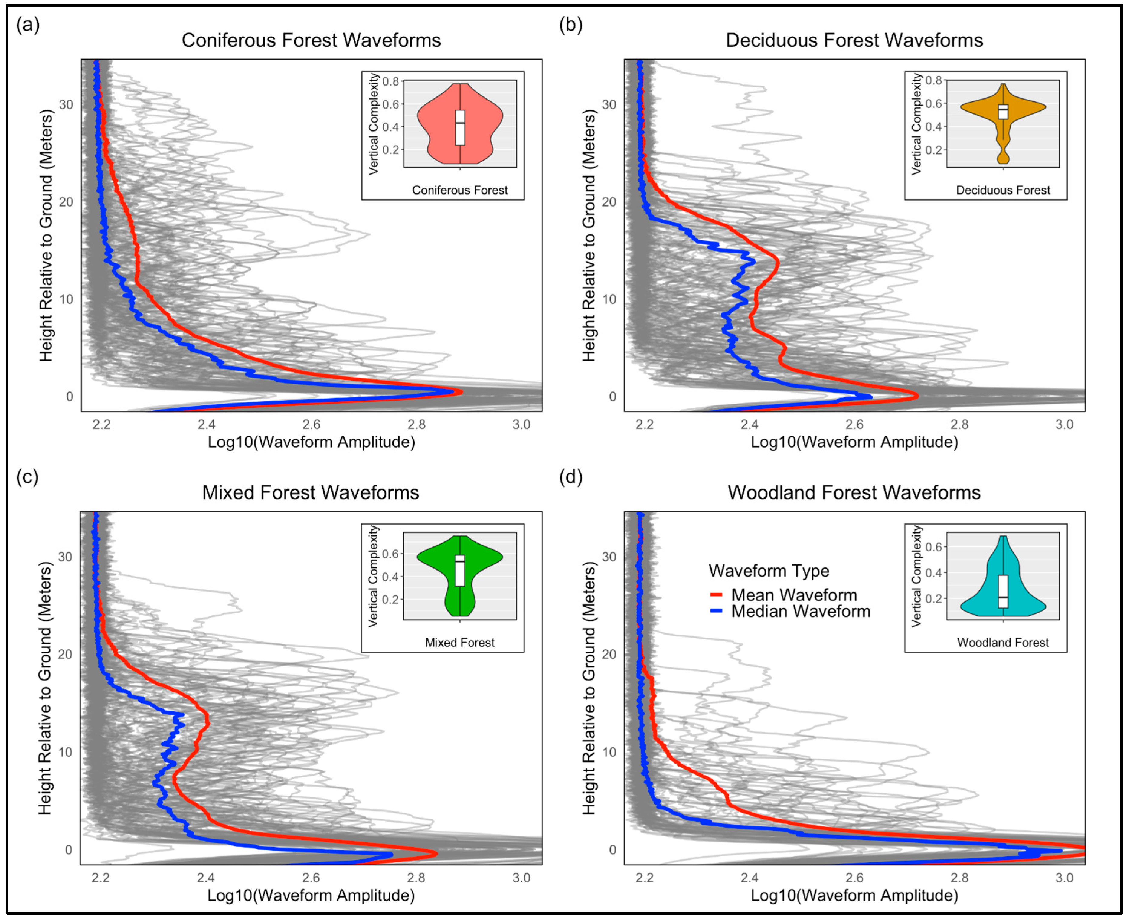
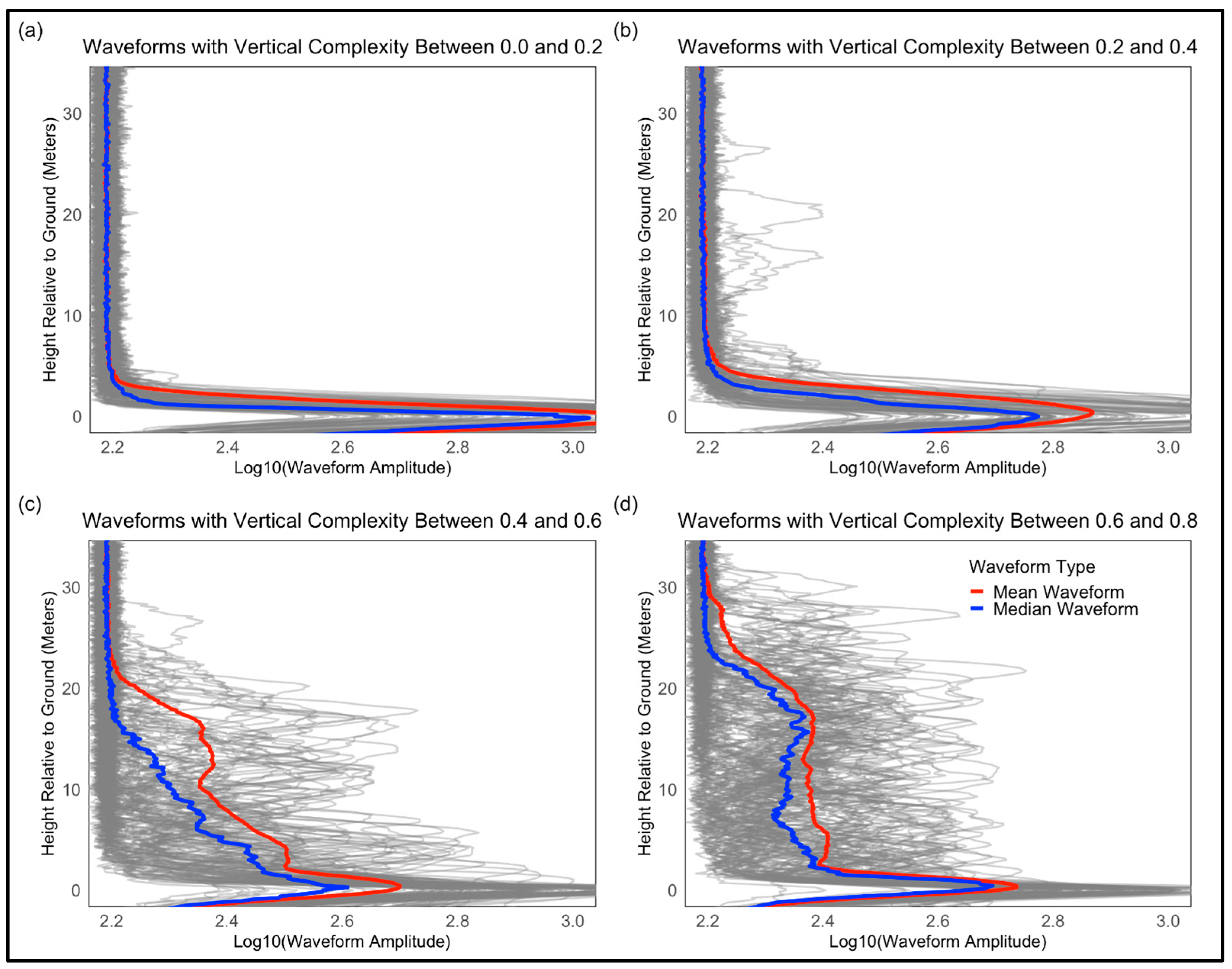
A total of 100 waveforms were randomly selected for each of the coniferous, deciduous, mixed, and woodland forests to visually depict the different waveform properties of these PFTs. The mean and median were calculated for each of the 100 waveform PFT clusters to identify broad trends in the vertical structure of each PFT. The 100 VC values associated with those waveforms were also visualized to directly connect waveform structure to VC for each PFT. A separate analysis randomly selected 100 waveforms from four bins of VC values (0.0–0.2, 0.2–0.4, 0.4–0.6, 0.6–0.8), and studied the structure of those waveforms. Mean and median waveforms were calculated for each VC bin to identify the underlying waveform structures associated with each value range.

3.3. LiDAR Stratified Sampling

This study used 93 LVIS flightlines from 2017 and 2019. Six flightlines were selected for model validation and were excluded from any analyses (Figure 1). We spatially stratified our flightline selection using the ABoVE B-level Standard Reference Grid to capture the full range of environmental and ecological conditions in the ABoVE Domain [60]. For each B-level tile, we chose one flightline from 2017 and one from 2019 when both years were available. If only one year was present, we selected a single flightline from that year. This sampling routine resulted in 93 flightlines dispersed evenly throughout the ABoVE Domain.
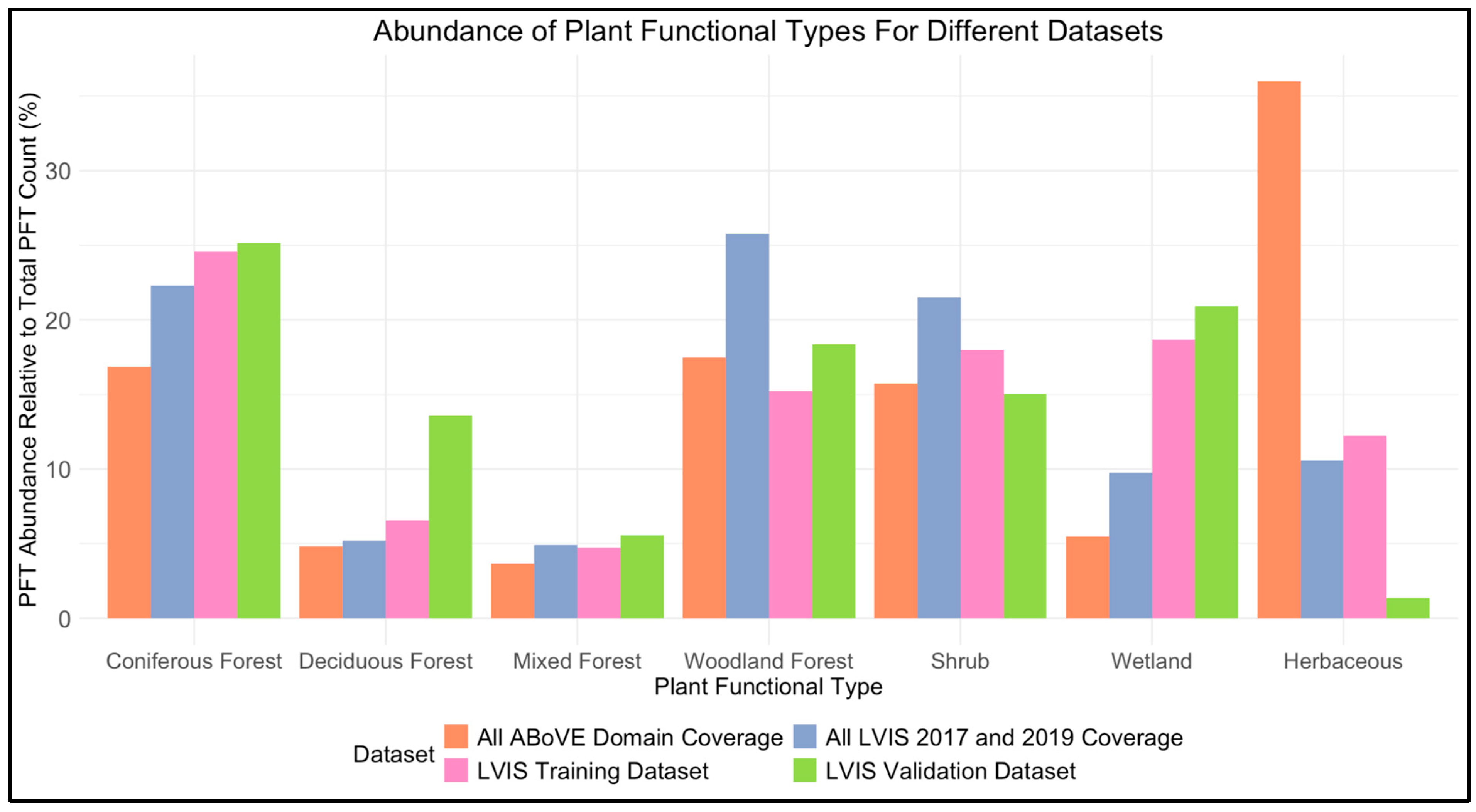
We compared the distribution of PFTs across the entire ABoVE Domain to those within various subsets of the available LVIS flightlines in the region. These subsets included all the LVIS flightlines from 2017 and 2019, the LVIS flightlines used for model training, and the LVIS flightlines reserved for validation. The purpose of this comparison was to assess the correspondence between the LVIS datasets and the ABoVE domain using the PFT abundances from the ABoVE-LULC dataset across the entire ABoVE Domain as a baseline. Figure 2 depicts this comparison.
In the ABoVE Domain, the herbaceous PFT is the most abundant, followed by coniferous and woodland forests. Deciduous and mixed forests, along with wetlands, are the least abundant PFTs, and each account for less than 6% of the land cover. All three LVIS datasets in Figure 2 significantly underrepresent the herbaceous cover of the ABoVE Domain. LVIS datasets also overrepresent wetland abundance in the ABoVE Domain by factors ranging from 2 to 4, although this issue is worse with the LVIS training and validation datasets. The LVIS training and validation datasets represent woodland forest and shrub abundance in the ABoVE Domain better than the entire 2017 and 2019 LVIS datasets. While the complete LVIS 2017 and 2019 datasets better represent ABoVE Domain PFT distributions compared to the spatially stratified LVIS training and validation datasets, they are still not a perfect representation of the ABoVE Domain.

3.4. Plant Functional Type Groupings

The ABoVE-LULC dataset was aggregated to produce a set of optically derived PFTs. We omitted water, littoral, and barren land covers from analyses because they are primarily flat surfaces with a theoretical complexity value of 0 (and in practice are always less than 0.2). The remaining 12 land covers were grouped into seven PFTs (see Table 2). The ABoVE-LULC dataset specifies a range of canopy heights for each vegetation class [68]. We removed any LVIS footprints with canopy heights beyond the determined height range of their corresponding PFT grouping (height ranges in Table 2). The original ABoVE-LULC land cover classes, PFT groupings, NEON growth groups, and PFT height ranges are listed together in Table 2.

3.5. Green Season Length

The ABoVE-Pheno and MS-LSP algorithms define spring and autumn onset as the first and second dates of the annual half-maximum of the Enhanced Vegetation Index (EVI), respectively [28,70]. Therefore, the green season length can be calculated as follows:
Green Season Length (Days) = Autumn Onset (DOY) − Spring Onset (DOY)
We calculated Long-Term Green Season Length (LTGSL) using Long-Term Spring Onset (LTSO) and Long-Term Autumn Onset (LTAO) from the ABoVE-PHENO dataset. We also calculated Annual Green Season Length (AGSL) using Annual Spring Onset (ASO) and Annual Autumn Onset (AAO) from the MS-LSP dataset. Pearson correlations between phenological variables and VC were calculated. The relationships between phenological variables and VC were studied across and within PFTs using LOESS lines.

3.6. HLS Optical Data

HLS mean mosaics were produced by merging every viable scene in a forty-day window centered around each LVIS flightline collection date. HLS scenes with less than 80 percent cloud cover and greater than 20 percent spatial coverage were considered viable. The HLS mask product, Fmask, was applied to each HLS scene before mosaicing [75]. Mosaicing ensures that a stable optical signal corresponds to each VC measurement. The Normalized Burn Ratio (NBR) and Normalized Difference Vegetation Index (NDVI) were calculated for each mosaic. Pearson correlations between HLS spectral bands and spectral indices (blue, green, red, NIR, SWIR1, SWIR2, NBR, NDVI) and VC were calculated. Using LOESS lines, the relationships between HLS variables and VC were studied across and within PFTs.

3.7. Environmental Variables

Annual accumulated precipitation (PRCP) and median annual maximum daily temperature (MAT) for 2017 and 2019 were derived from the Daymet Version 4 R1 daily temperature and precipitation variables. Median annual minimum daily temperature, mean annual maximum daily temperature, and annual minimum temperature were also calculated for inclusion in the VC retrieval modeling (see Table 1 and Table 2). Annual climate variables are used here to stabilize daily meteorological estimates as they correspond to the longer periods that determine vegetation growth. Pearson correlations between climate variables and VC were calculated across all PFTs. The sensitivity of VC to climate variables was studied across and within PFTs using LOESS lines.
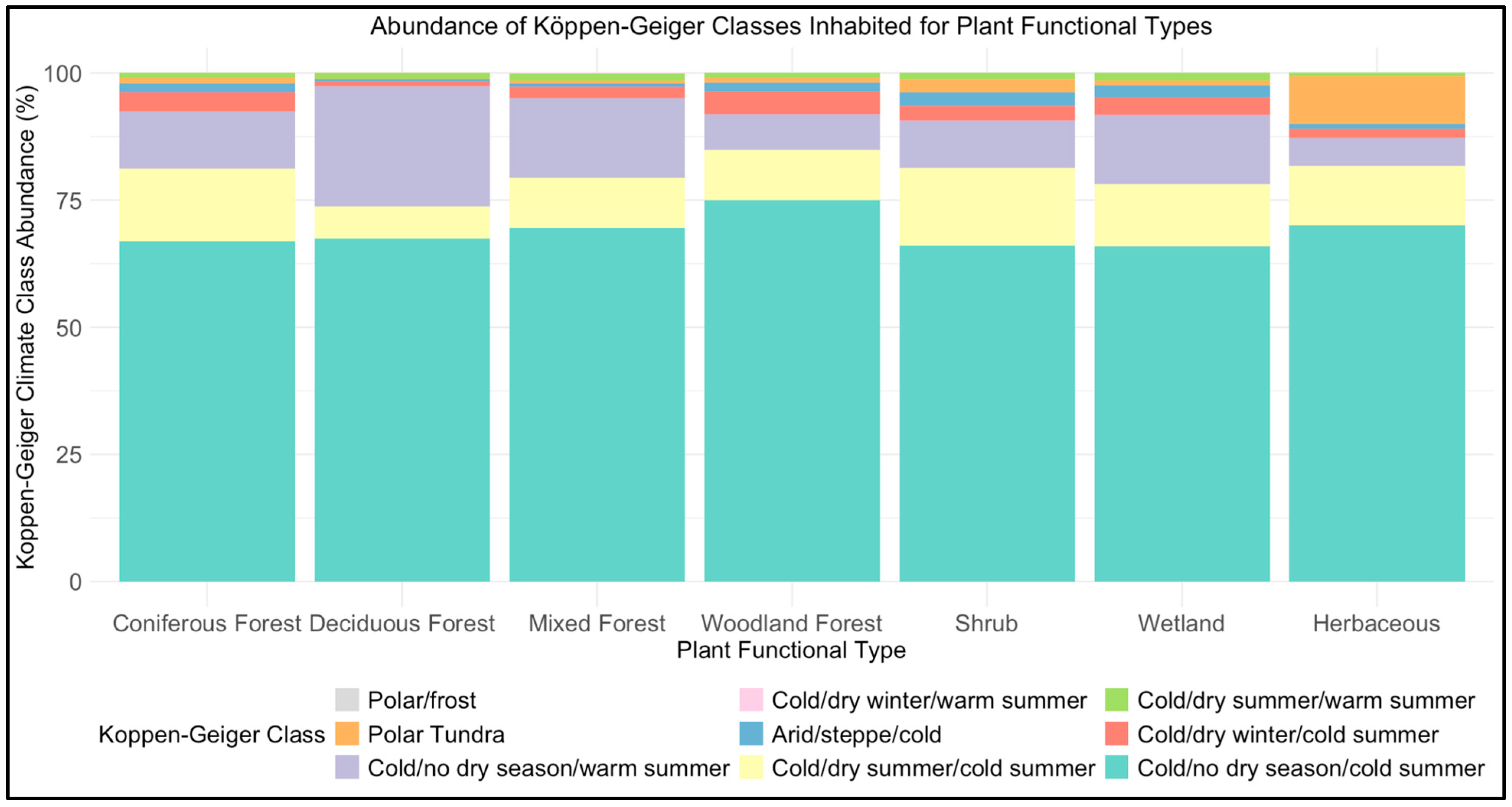
Köppen–Geiger classes and ABoVE-LULC PFTs were sampled within the bounds of every LVIS flightline from 2017 and 2019 in the ABoVE domain. The distribution of Köppen–Geiger classes occupied by each ABoVE-LULC PFT was calculated. By using a global climate classification system, this analysis intended to lend a global context to the climate–VC patterns that were observed throughout the ABoVE Domain in this study. The Köppen–Geiger classes also help to integrate the results of this study with other global studies focused on forest structural complexity and hydroclimate.

3.8. Modeling, and Validation

Our modeling experimental design has two aims: (1) to study the potential of different variables for predicting VC in the ABoVE Doman; (2) to investigate the effect of the validation methodology on perceived model robustness. These aims guide our choices for predictor variable configurations, training data sampling methodology, and validation methodology.
We trained four random forest regression models to predict VC using the R randomForest package [76,77,78]. The predictor variable configurations for each random forest model are listed in Table 3, but can be described as follows: (1) Model A uses long-term and single-year variables; (2) Model B uses single-year variables, but no long-term variables; (3) Model C uses long-term and single-year variables, but only uses predictor variables with Pearson correlation coefficients less than or equal to 0.70; (4) Model D uses no phenological variables.
All four random forest models had 300 decision trees, used two variables at each split (a hyperparameter known as ‘mtry’ in the randomForest R package, which controls the number of variables for each split), and were trained on the same dataset. Low mtry values were used to stabilize RFs by reducing the correlations between trees and exploiting information from less important variables [79]. The training dataset was sampled from the LVIS flightlines that were used for analysis. A spatial sampling routine ensured that training data points were separated by 500 m, in imitation of a previous study in the ABoVE Domain [80]. Spatially separated sampling drastically reduces the training dataset size but helps to mitigate the effects of spatial autocorrelation. The minor performance costs associated with a reduced training dataset are acceptable because this study does not seek to publish a new VC map product. Instead, it examines the relationships between VC, hydroclimate, and optical variables to understand the feasibility of such a mapping.
Each model was evaluated using k-fold cross-validation (five folds) and two separate validation datasets. The first validation dataset (SampVal) was produced by reserving 20% of points from within the sampled training dataset. SampVal represents a traditional validation approach that draws on data from locations where the model was trained. The second validation dataset (FLVal) used the six reserved LVIS flightlines. In contrast to SampVal, FLVal presents data from regions external to those used in training the model. FLVal is an application of spatial cross-validation to ensure genuine model robustness. Model performance during validation was evaluated using R-squared, mean absolute error (MAE), and root–mean–square error (RMSE).

4. Results

4.1. Plant Identity, Canopy Height, and Vertical Complexity

The five original NEON growth forms (Figure 3a) can effectively be divided into two canopy height categories represented by the mature tree and shrub growth groups. Height increases with maximum crown diameter (MCD), but some of this relationship is explained by a shift from the shrub to the mature tree growth group (Figure 3b). Height increases with stem diameter (SD) across and within growth groups (Figure 3c). Notably, the height–SD relationship becomes increasingly uncertain for mature trees (Figure 3c). This uncertainty is partially explained by the divergent heights of white spruce, quaking aspen, Alaska birch, and black spruce at greater SDs (Figure 3d), whereas these four taxa have significant overlap in height–SD trends between SDs of 5 and 10 cm. Height is consistently related to plant structural attributes, but these relationships are non-linear and vary among taxa and growth groups.
Canopy height rarely exceeds 20 m and VC rarely exceeds 0.6 in the ABoVE Domain (Figure 4). VC increases logarithmically with canopy height generally, but this exact relationship is not present within some PFTs. Shrubs, wetlands, and herbaceous PFTs may reach a relatively high VC (>0.4), but their heights are more linearly related to VC. Deciduous, coniferous, and mixed forests span the entire logarithmic relationship between VC and canopy height, but this becomes increasingly uncertain at higher VCs. Individual forest classes (coniferous, deciduous, and woodland) do not have distinct VC–height relationships.
PFTs have different distributions of VC values, with distinctions between forest and non-forest PFTs being the most dramatic (Figure 5). Still, between PFTs, there are significant overlaps in VC value distributions. No PFTs cover the entire observed range of VC values, although forest VC is significantly more variable than non-forest VC (Figure 5). Coniferous, deciduous, and mixed forests have median VCs of 0.40, 0.49, and 0.474, respectively. VC distributions are better constrained for deciduous and mixed forests than they are for coniferous and woodland forests. The median VCs of the shrub, wetland, and herbaceous PFTs are 0.12, 0.16, and 0.13, respectively. Woodland median VC (0.32) sits between forest and non-forest PFTs and has a wide distribution of likely VCs.

4.2. LiDAR Waveforms, Plant Functional Types, and Vertical Complexity

Figure 6 shows LiDAR waveforms and distributions of VC values for the coniferous, deciduous, mixed, and woodland forest PFTs. The coniferous forest PFT had the greatest number of canopies over 20 m tall and displayed a gradual decline in return energy amplitude as height increased within the canopy (Figure 6a). Relative to mixed and deciduous forests, energy was distributed evenly throughout the coniferous PFT canopy (Figure 6a). The deciduous forest PFT had fewer canopies taller than 20 m, but greater average return energy amplitudes than the coniferous forest PFT (Figure 6b). In the deciduous forest PFT mean waveform, there were two local maxima, with one occurring in the understory at around 5 m and another in the upper canopy at around 15 m (Figure 6b). The mixed-forest PFT mean waveform contained a pronounced upper-canopy return energy peak at a height of around 15 m that was comparable in amplitude to the upper-canopy return energy peak of the deciduous forest PFT (Figure 6b). Unlike the deciduous forest PFT, the mean waveform for the mixed forest PFT contained no understory peak in return energy (Figure 6b,c). The woodland forest PFT canopies rarely exceeded 20 m, and the return energy distribution of their mean waveform resembled the return energy distribution of the coniferous forest PFT (Figure 6a,d). The violin plots demonstrating VC value distributions for each PFT for the subset of waveforms in Figure 6 are similar to those in Figure 5, which are representative of the entire ABoVE Domain.
Figure 7 shows LiDAR waveforms within different ranges of VC values. LiDAR waveforms with VC values between 0.0 and 0.2 contain no clear features beyond the ground return (Figure 7a). Between VC values of 0.2 and 0.4, waveforms begin to have features that are solely attributable to vegetation, and canopies as tall as 20 m (Figure 7b). The amplitudes of the peaks in the individual waveforms of this range are lower than those in the coniferous, deciduous, mixed, and woodland forest PFTs (Figure 7b). Waveforms with VC values between 0.4 and 0.6 rarely contain canopies taller than 25 m, but their return amplitudes are similar to those of the four forest PFTs (Figure 7c). The average waveform in this range displays clear return energy peaks in the understory and upper canopy at around 5 and 15 m, respectively, with return energy decreasing as height within the canopy increases (Figure 7c). Return energy is distributed most evenly throughout the canopy in waveforms with VC values between 0.6 and 0.8 (Figure 7d). In comparison to waveforms with VC values between 0.4 and 0.6, the mean waveform in this range has lower understory return energy amplitudes, but comparable upper-canopy return energy amplitudes (Figure 7c,d).

4.3. Environmental Sensitivities of Vertical Complexity

VC is sensitive to mean annual temperature (MAT) across and within PFTs, but not to PRCP. Maximum potential VC increases with MAT, but a higher MAT does not guarantee a high VC (Figure 8a). The consistently low VCs of shrub, wetland, and herbaceous PFTs along the gradient of MATs demonstrate that some of the moderate positive correlation between VC and MAT (r = 0.45) can be attributed to shifting PFT abundances (Figure 8a). However, the VC of individual forest PFTs is directly sensitive to changes in MAT. Deciduous and mixed-forest VC is the most sensitive to MAT, whereas coniferous forest VC varies far less with MAT (Figure 8a). In contrast to temperature, there is no obvious relationship between PRCP and VC across or within PFTs. The relationship between MAT and VC involves both shifts in PFT abundances and alterations in individual PFT growth patterns.
The entire LVIS ABoVE 2017 and 2019 dataset covered 9 out of the 30 global Köppen–Geiger climate classes (Figure 9). For every PFT, the “cold/no dry season/cold summer” (“Dfc” in the Köppen–Geiger system—light blue in Figure 9) was by far the most commonly inhabited climate zone. Importantly, the Dfc class is characterized by consistently cold temperatures but contains no dry season. Most Köppen–Geiger classes accounted for insignificant portions of the LVIS dataset. The nine classes covered by the LVIS ABoVE dataset represent a small portion of the global climate variability that is described in the Köppen–Geiger classification system. Furthermore, the distribution of those nine climate classes is dominated by a single Köppen–Geiger class.

4.4. Phenology and Vertical Complexity

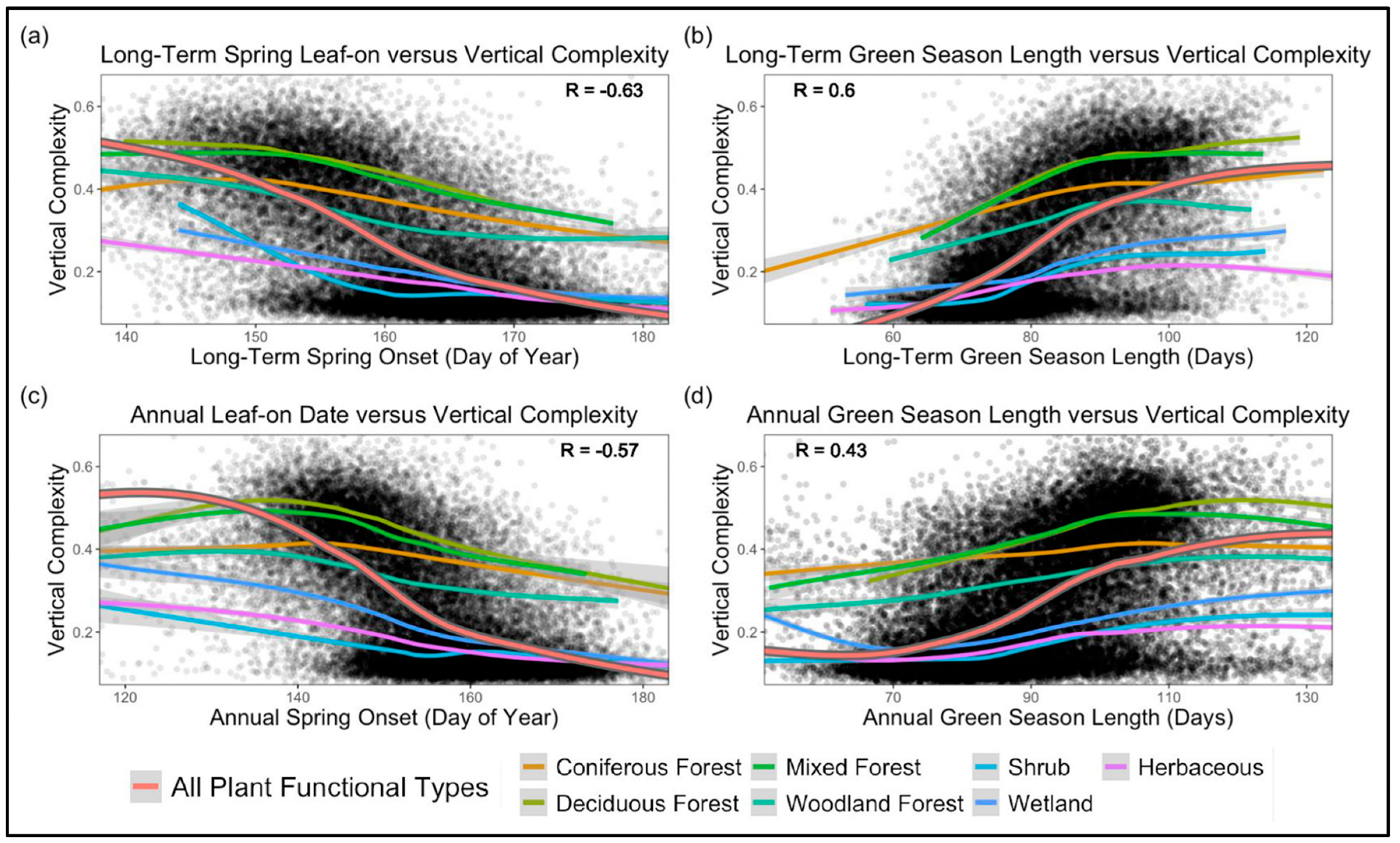
VC was associated with the timing and length of phenological events, as determined by the MS-LSP and ABoVE-Pheno algorithms (Figure 10). Later spring onsets were associated with lower VCs (Figure 10a,b), while longer green season lengths were associated with higher VCs (Figure 10c,d). Long-Term Spring Onset (LTSO) was only slightly more correlated to VC (r = −0.63) than annual spring onset (ASO) (r = −0.57). Long-Term Green Season Length (LTGSL) was significantly more correlated to VC (r = 0.60) than Annual Green Season Length (AGSL) (r = 0.43), meaning that green season length depends on long-term averages for its relationship with VC to emerge. Spring onset had stronger associations with VC than green season length for long-term and annual variables. The universal relationship between spring onset and green season length is not reflected in every PFT. The VC of non-forest PFTs is generally not sensitive to phenology, though wetland and shrub VC increases with LTGSL (Figure 10b). Deciduous and mixed-forest VC does vary with phenological variables, but coniferous phenologies are less indicative of VC (Figure 10b,d). Spring onset and green season length have very similar correlations to VC, likely because these two phenological variables are closely related. Optical phenological variables are generally related to VC, but PFTs are necessary to understand these relationships in detail.

4.5. Canopy Optical Properties and Vertical Complexity

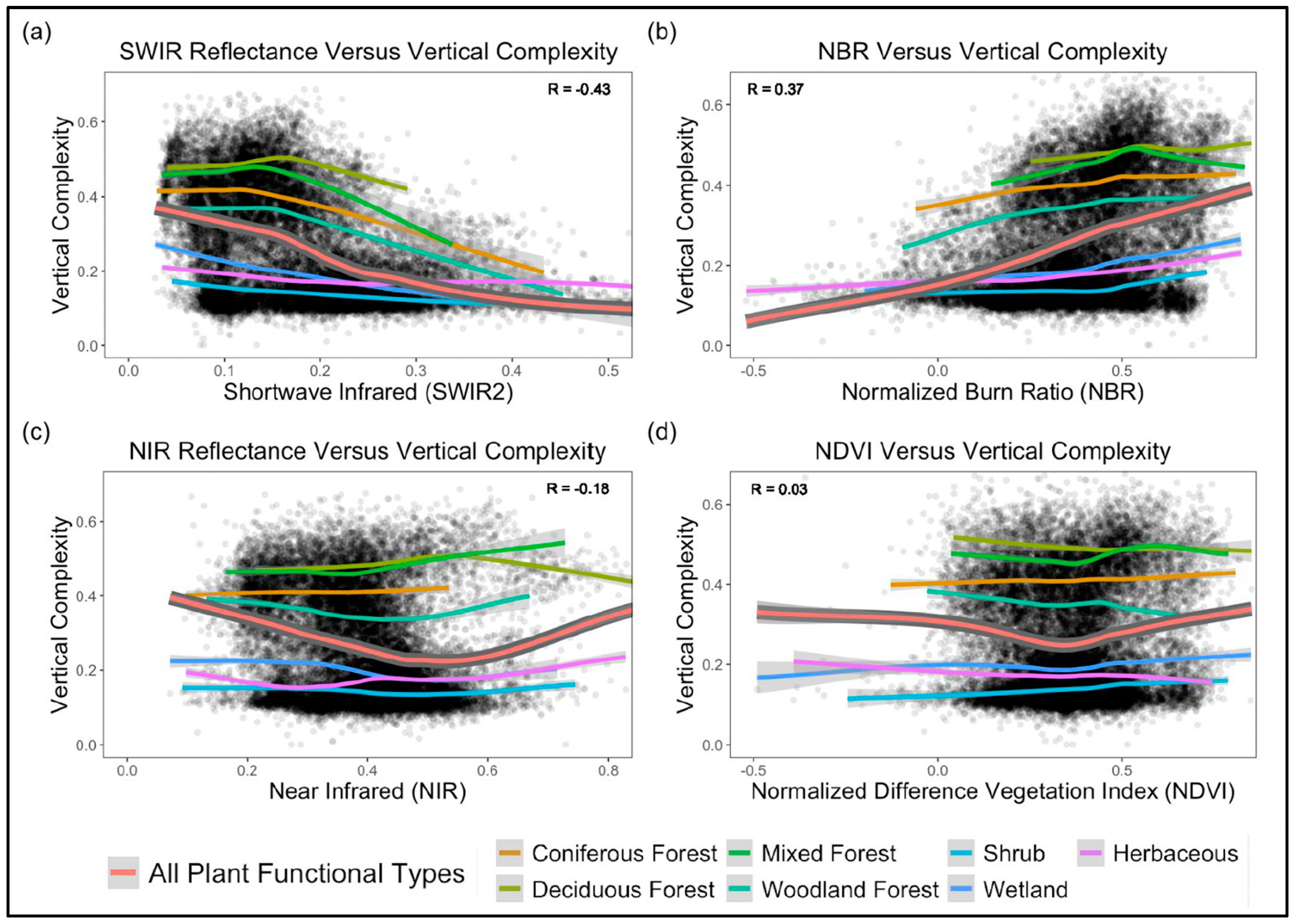
Canopy optical reflectance has a relatively limited relationship with VC, but shortwave infrared reflectance (SWIR2) was the most correlated with VC of any HLS variable (r = −0.43) (Figure 11a). In contrast, canopy NIR reflectance is not sensitive to vertical complexity (r = −0.11). These single-band relationships impact vegetation index sensitivities such that the Normalized Burn Ratio (NBR) increases with vertical complexity (r = 0.37), but NDVI does not (r = 0.01) (Figure 11b,d). Canopy SWIR2 reflectance decreases with canopy vertical complexity across all PFTs, which is partially a result of distributional shifts from high-VC to low-VC PFTs. Regardless, the SWIR2 reflectance of mixed, coniferous, and woodland forests are individually sensitive to VC (Figure 11c). Non-forest SWIR2 reflectance also gradually declines with increasing VC. Although the within-PFT sensitivity of HLS variables to VC is low, the same optical reflectance value corresponds to significantly different VCs across all PFTs (Figure 11d), This variability highlights the challenges of retrieving structural parameters using optical reflectance.

4.6. Random Forest Predictions

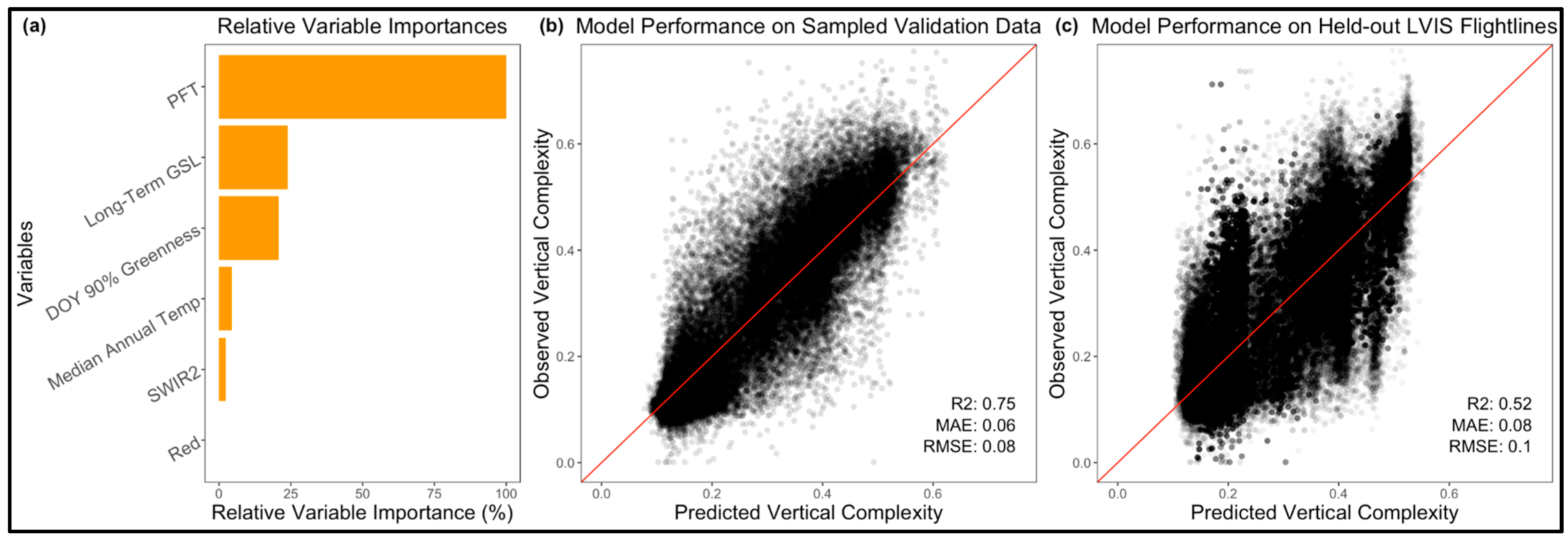
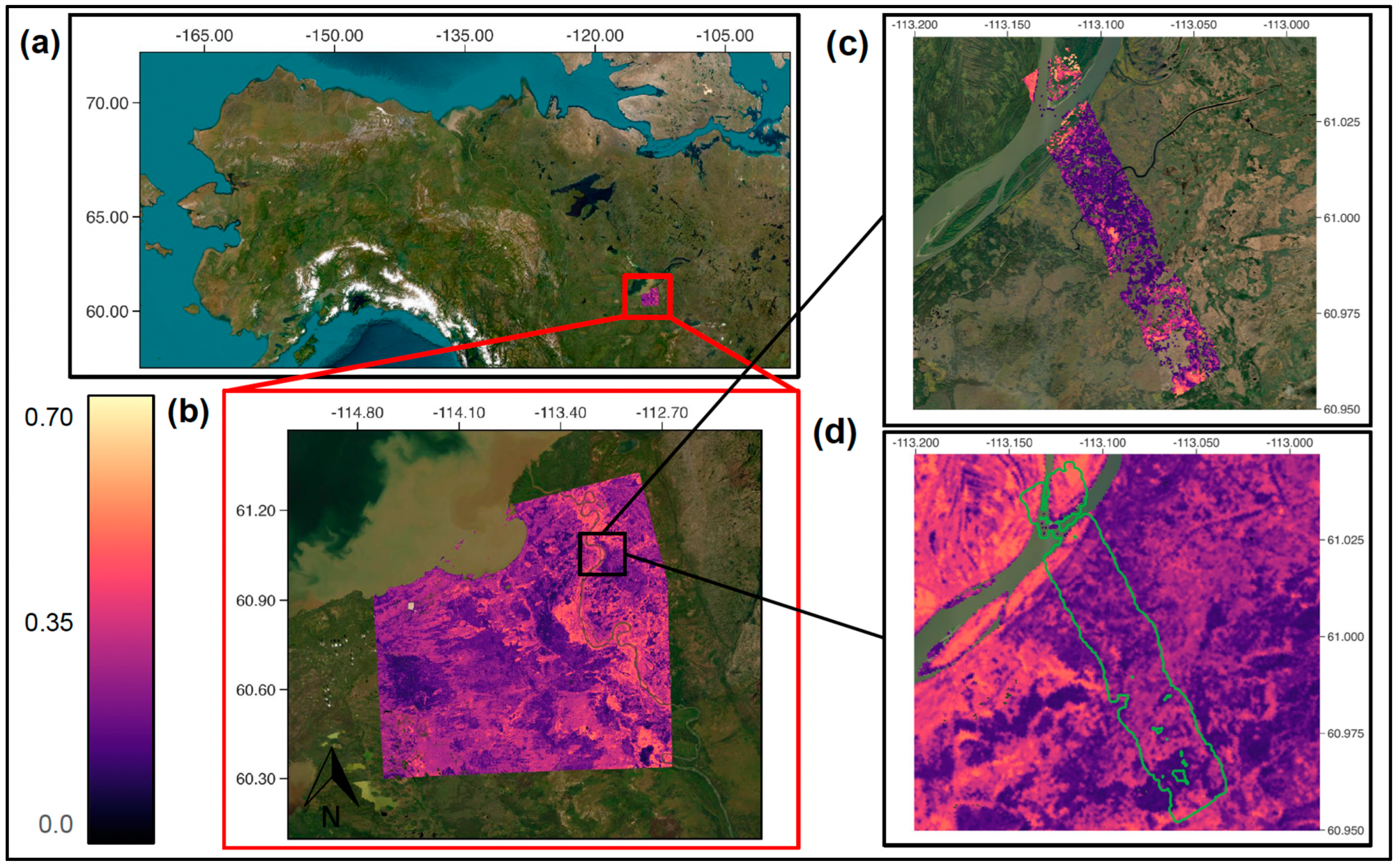
All four random forest models performed well during k-fold cross-validation and SampVal validation (see Table 4). Although each model was trained on spatially separated data, they all performed poorly on the fully external FLVal validation dataset (see Table 4). Model C (Figure 12a,c) performed slightly better on the FLVal than the other three models (Figure 12c; Table 4) but had the worst performance during k-fold cross-validation and SampVal validation (Figure 12b; Table 4). PFT was the most important predictor variable for all four models, so the relative importance (RI) of the other predictor variables is quantified as a percentage relative to PFT. Phenological variables had the second highest RIs for Models A, B, and C (Model A: LTGSL = 46.85%, Model B: ASO = 26.38%, Model C: LTGSL = 23.87) (see Table 4). SWIR2 had the second highest RI in Model D (SWIR2 = 16.23%), which used no phenological variables and performed the worst on FLVal (R2 = 0.38). AGSL had a notably lower RI in Models A and B compared to ASO, LTGSL, and LTSO (see Table 3). NIR, Red, NBR, and PRCP had essentially no RI in any of the four models (see Table 3). Despite learning the patterns of VC across the ABoVE (Figure 13), all four random forest models were not robust to validation on entirely new regions.

5. Discussion

In this study, we evaluate the LVIS LiDAR waveform complexity variable to gain a more physical understanding of the vegetation structural metric in light of complex phenological and hydroclimatic variability. This discussion section reflects on the results, identifies the limitations of this work, and suggests recommendations for future studies on vegetation structural metrics.
  • The relationship between canopy height and VC
The vegetation vertical complexity (VC) metric has a logarithmic relationship with canopy height and LiDAR scattering “counts”; as such, it is unclear if the VC metric accurately describes biophysical vegetation growth or fits diverse PFTs structures into a single expected relationship. The divergence between VC and canopy height in high-VC canopies demonstrates the complementarity of both variables, as not all tall canopies have a high VC, and not all vertically complex canopies are tall. Unlike previous studies [81], we did not observe PFT-specific height–complexity relationships for the forest PFTs. The forest PFTs used in this study did have different VC–height patterns than non-forest PFTs, demonstrating that these relationships can be used to separate broad structural growth forms. While deciduous forests are the most vertically complex and have the narrowest distribution of VC values, the coniferous and woodland forest PFTs have more variability, demanding greater caution in inferring structure from these classes.
We show, through a modest analysis of the NEON in situ plant structure variables—plant height, stem diameter, and maximum crown diameter—that universal vegetation structural relationships must be studied across and within structurally meaningful groupings of plants. We identified an increasingly uncertain relationship between plant height and stem diameter in the mature tree growth group, which could be attributed to species-specific growth patterns in the NEON data. This component of our analysis demonstrates that the construction and conception of multi-taxa categories have important implications for any analysis of plant structure. Different satellite-derived PFTs from the ones used in this study may partition these universal structural relationships differently, leading to different results.
  • Waveform structure and vertical complexity
Full-waveform analysis provides insight into the vertical structure of different optical PFTs that a derived summary metric alone, such as VC, cannot. Deciduous and mixed forest PFTs contain dense upper canopies and understories, while the coniferous forest PFT has a notably even distribution of return energy throughout its canopy. Other full-waveform summary metrics that capture these differences would be complementary to VC in lending structural significance to optical PFTs. By demonstrating that ground returns produce average VC values of around 0.2, we identify an important lower limit for the interpretability of VC values. Any analysis of VC values below 0.2 should not expect forest vegetation to be present, although some cases of sparse vegetation and short grasses are still probable.
  • Phenology and VC
By linking optical phenology to VC, our study provides a set of mechanistically interpretable satellite variables for monitoring vegetation structure. Rather than using annual maximums, as in other studies [45], our study links phenological events such as spring onset and green season length to vegetation structure. While these variables do not directly retrieve canopy optical properties, they signify the annual period afforded to vegetation for photosynthesis and biomass accumulation. Because phenology represents precisely how diverse vegetation species are responding to climate change, it reflects broader hydroclimate variability including covarying temperature, precipitation, soil moisture, and evaporation. This is evidenced by long-term spring onset being more correlated with VC than mean annual temperature. The phenology variables in this study offer new ways to connect climate change to vegetation structure across the boreal region.
  • Climate and VC
Our analysis found temperature to be the defining climatic variable for VC throughout the ABoVE Domain. This finding conflicts with research identifying water availability as the primary driver of vegetation structure [11,13], although temperature may have an outsized effect at high latitudes where cold winters determine growing seasons. The Köppen–Geiger analysis highlights the importance of the study domain for interpretations of climatic results. Nearly 70% of the data points used in our study across all PFTs came from a single Köppen–Geiger climate class characterized by cold temperatures and a lack of a dry season (Dfc). Global studies of forest structure will cover a far greater range of hydroclimatic conditions, many of which are defined by water availability rather than cold temperatures.
The interplay between latitude, elevation, and vegetation structure is mediated by temperature, soil quality, and hydrology. Maximum annual temperature (MAT) complements topographic and latitudinal data by offering a direct link between a dynamic climate variable and VC in the boreal region. The observed MAT-VC relationship suggests that future warming due to climate change may increase the maximum potential VC in the ABoVE Domain by enhancing the VC of forests and triggering transitions from non-forest to forest PFTs. Previous research that employed the ABoVE-LULC dataset to track changes in PFT abundance throughout the ABoVE Domain found an annual change of 0.44% per year for the period 1984–2014 [61]. Future climate projections of a warmer Arctic suggest a more rapid pace of PFT transitions.
  • Random forest predictions of VC
It has become clear that model performance metrics can be inflated by spatially autocorrelated training data and a lack of spatial cross-validation [59,82,83]. Our study responds to this problem by implementing spatial cross-validation alongside traditional validation methods. Our findings suggest that spatially separating training data points and applying traditional validation methods is insufficient for assessing prediction performance in RF models, due to samples being spatially autocorrelated even at coarse scales. We imitated the sampling and validation routines of a previous study that had successfully predicted VC across the ABoVE Domain [45]. Using these methods, our models performed comparably well (R2 = 0.75–0.80). However, when we tested all four models’ ability to predict VC in entirely new regions, we observed considerable reductions in model performance. This comparative analysis of different validation methods confirms the assumption that random forest models may be useful for imitating ecological patterns but can fail to produce generalizable outputs of LiDAR structural variables.

5.1. Study Limitations

5.1.1. Spatial Sampling of LVIS Flightlines

This study used 93 LVIS flightlines for model training and analysis, which represents a small fraction of the total number of available LVIS flightlines in the ABoVE Domain. We sought to mitigate this by sampling across a broad and representative region. A comparison of PFT distributions in these 93 flightlines and the entire LVIS 2017 and 2019 datasets found that neither dataset was fully representative of those across the entire ABoVE Domain, indicating a selection bias inherent to the available data. Without explicit efforts to represent the PFTs of the ABoVE Domain evenly, the 1.8 km swath width and the 10 m footprint diameter make LVIS datasets susceptible to bias. Some of the observed model performance reduction in unseen regions can be attributed to spatial autocorrelation and a small training dataset. Still, PFT abundance analysis indicates that if mapping the entire ABoVE Domain is the objective, any validation dataset that is randomly derived from the entire LVIS 2017 and 2019 dataset will differ in PFT distribution from the entire ABoVE Domain. Models that use PFT as a predictor variable will be sensitive to these differences.

5.1.2. Summer-Only LiDAR Observations

The LVIS ABoVE missions only measured VC in the summer during leaf-on conditions. This leaves uncertain the degree to which the leafy versus woody components of vegetation structure contribute to VC, and if these relative contributions vary by PFT. This represents a significant gap in our understanding of how different aspects of physical vegetation structure relate to moderate-resolution VC. A lack of seasonal LiDAR observations also prevents the further study of optical phenological signals as they relate to VC. This study could compare phenological variables in the spring and the fall to VC in the summer, but multi-temporal VC data would enable direct comparisons throughout the year.

5.1.3. Temporal Misalignment between PFT and LiDAR Datasets

We compared a PFT dataset from 2014 to LiDAR data from the summers of 2017 and 2019. Temporal misalignment between the PFT and LiDAR datasets, and the predicted nature of the PFT classes, introduce uncertainty into our analysis. During the 31-year period of the ABoVE-LULC dataset, there was a 13.6 ± 1.3% change in land cover [61], which amounts to an average change of 0.44% per year, and a 1.3–2.2% change from 2014 to 2017 and 2019. The observed rates of land cover change in the ABoVE Domain from 1984 to 2014 suggest that the 3–5-year temporal misalignment between the ABoVE-LULC and the LVIS datasets is not a significant source of error. Therefore, the distributions of VC within each ABoVE-LULC PFT class are representative of the distributions of VC that would be found in an updated dataset.

5.1.4. Drawbacks to Modeling at 30 m Resolution

While our use of moderate-resolution satellite data is acceptable for drawing broad conclusions about vegetation in the boreal region, this approach has limitations. In contrast with high-resolution and in situ data, moderate-resolution PFT maps are more likely to contain mixtures of multiple vegetation types within a single pixel. This sub-pixel heterogeneity can erode the consistency of the relationship between physical structure and optical observations. This uncertainty also translates into moderate-resolution phenology datasets, which treat the phenology of each forest stand as a single signal. In reality, plant phenology can vary depending on the vertical location within a forest stand [84]. Optical satellite phenology algorithms are sensitive to understory and overstory phenological signals but do not distinguish between them. Another drawback of moderate-resolution data is evidenced by the lack of distinct height–VC relationships, which are present in in situ datasets, but not in the coniferous, deciduous, and mixed forest ABoVE-LULC PFTs [81].

5.2. Recommendations

5.2.1. Improved Spatial Sampling

Studies with sufficient computational resources could harness all LVIS data in the ABoVE, which amounts to several thousand flightlines. A less computationally intensive way of representing the entire LVIS dataset could use the R Structurally Guided Sampling (sgsR) package to select spatially distributed points from within every LVIS flightline [80], resulting in a smaller dataset that still represents every LVIS flightline. However, the LVIS ABoVE campaign flightlines were intended to correspond with other airborne and in situ datasets or to study particular ecosystems, but they are not representative of the entire ABoVE Domain. Whenever possible, future studies should use maximally representative datasets of the ABoVE Domain. We also recommend that future airborne campaigns are designed to be more representative of the diverse PFTs and land covers in the ABoVE domain.

5.2.2. Further Experiments with Optical Methods

Further experimentation with optical reflectance variables may yield better retrievals of VC. Variables describing averages and trends in multi-year reflectance values for specific PFTs would reflect the long-term growth patterns that result in vertically complex canopies. Previous work has established relationships between optical texture variables and vegetation’s structural complexity [3,46]. Texture variables describe different surface properties from optical reflectance values and do not suffer from spectral saturation [3,46]. Finally, single-date reflectance variables corresponding temporally to VC measurements would reduce the uncertainty introduced by the multi-week mosaics used in this study. Future work should explore the range of optical techniques used for retrieving biomass and canopy height to determine which methods apply to retrievals of VC and which do not.

5.2.3. Potential for SWIR Phenology

Determining the sensitivity of canopy optical properties to VC is essential for its retrieval and monitoring. NIR was not sensitive to VC, but we observed a moderate negative correlation between SWIR2 reflectance and VC that may be mediated through vegetation water content [85]. VC had a limited correlation with NDVI, which primarily reflects leaf chlorophyll content. However, the relationship was much stronger between VC and the normalized burn ratio (NBR), which detects both chlorophyll and leaf water content via its SWIR2 component. The sensitivity of SWIR to VC suggests that current phenological algorithms could be better tailored for assessing VC variability. While phenological timing variables from MS-LSP and ABoVE-Pheno had the highest correlations with VC, these algorithms rely on the enhanced vegetation index (EVI), which is a fundamentally NIR-based vegetation index. Phenological timing variables derived from SWIR-based metrics may carry stronger associations with VC and would complement NIR-based timing variables.
The annual maximum reflectance variables that accompany phenology datasets would be more applicable to predicting VC if they included SWIR or SWIR-derived indices. In contrast, maximum annual EVI from the ABoVE-Pheno dataset had only moderate importance in Model A. Maximum annual NBR and SWIR may also reflect peak annual VC better than HLS SWIR and NBR mosaics. Future work should focus on annual and phenological SWIR variables as they compare VC with a focus on complementary optical phenological signals.

5.2.4. The Need for Multi-Scale Analysis

A multi-scale analysis would help to establish high-confidence relationships between VC and ecological variables at higher resolutions and provide a foundation for understanding the retrievals of VC with all available sensors. LiDAR structural complexity metrics are highly scale-dependent, which complicates multi-resolution LiDAR variable comparisons [86]. Any multi-scale study will need to account for this dependency as it draws relationships between PFTs, optical reflectance, and VC. NEON field sites provide overlapping in situ PFT, high-resolution, airborne, full-waveform LiDAR and high-resolution airborne optical datasets that are essential for this kind of research. Many NEON sites also overlap with LVIS flightlines and footprints from the spaceborne Global Ecosystem Dynamics Investigation. Additionally, in situ phenology cameras in areas with LiDAR structural data would be highly complementary to satellite phenology variables.
The results of this study diverge with in situ studies of forest structural complexity. Whereas in situ research has found that tree species mixing enhances structural complexity through complementary crown architectures and resource needs [87], our study found purely deciduous forests to have higher VC than mixed forests. A multi-scale perspective is required to understand and integrate these diverging results.

6. Conclusions

Terrestrial, airborne, and spaceborne LiDAR sensors enable the production of novel methods for quantifying and studying vegetation structure, but each new metric must reflect an ecological meaning that can be ascribed to a physical quantity. Machine learning models can predict vegetation structure with satellite optical data to overcome the spatiotemporal limitations of LiDAR sensors, but may suffer from signal saturation, prediction uncertainty, and a failure to perform well in unseen regions. In this study, we evaluate a LiDAR waveform complexity metric with these issues in mind. Previous studies have linked global patterns of forest structural complexity to hydroclimatic and soil conditions [11,13]. While a recent study successfully predicted VC in the ABoVE Domain using Landsat optical variables [45], more work is needed to understand the ecological significance of these VC maps. In light of these previous examinations, we relate VC to widely available climatological, ecological, and optical variables, and by modeling VC with novel applications of existing optical variables. Our study contributes to a better understanding of VC in the ABoVE Domain, therefore improving the utility of its widespread prediction.
We identified relationships between phenology and VC that offer novel ways of monitoring vegetation structure using satellite data. Spring onset and green season length were moderately correlated with VC, and temperature was more correlated with VC than precipitation. We propose that integrating phenology, temperature, and PFT variables into satellite studies of vegetation structure will yield better explanations for the observed optical trends. The complementarity of phenological variables and vegetation indices stems from their different mechanistic relationships with climate and vegetation structure. The inconsistent performance of our random forest models, even with a spatially separated sampling routine, emphasizes the need for robust validation schemes to avoid overestimating model performance. Future research should identify the portion of VC that is optically detectable by analyzing seasonal variations in VC as they relate to leafy and woody vegetation components.
This study links the ABoVE-LULC classes to VC and finds that the vertical structure of these classes is sensitive to climate, offering new ways to connect climate change to vegetation structure across the boreal region. Additionally, phenological timing assessments outperformed HLS reflectances, providing alternative methods for retrieving vegetation structure. Understanding the interplay between VC, water content and shortwave infrared reflectance could enable new methods of tracking fire severity and post-fire structural recovery in the ABoVE.
Our study demonstrates that PFT, phenology, and climate can effectively predict patterns of VC in the ABoVE Domain. A primary motivation for mapping forest structure is the need to identify rapid and gradual structural changes from disturbances and climate change respectively. Rather than including geolocation in our model, we opted for ecologically interpretable and climatically dynamic variables. We observed PFTs to be the most important variable for predicting VC, confirming the structural significance of these functional types. Phenological timing variables outperformed HLS reflectance variables in our models and may offer an entirely different method of retrieving vegetation structure.

Author Contributions

D.J.: Conceptualization, methodology, software, formal analysis, investigation, data curation, writing—original draft preparation, writing—review and editing, visualization; R.B.: investigation, writing—review and editing. J.V.F.: conceptualization, software, writing—review and editing, supervision, project administration. All authors have read and agreed to the published version of the manuscript.

Funding

This research received no funding.

Data Availability Statement

All data presented in this study are publicly available as indicated in the materials and methods sections. Readers may contact the author with questions after reviewing the in-text links and citations.

Acknowledgments

We would like to thank Miriam Bartleson, Kelly Bonnville-Sexton, and Felix Yu for providing feedback throughout this study.

Conflicts of Interest

The authors declare no conflicts of interest.

References

  1. McElhinny, C.; Gibbons, P.; Brack, C.; Bauhus, J. Forest and Woodland Stand Structural Complexity: Its Definition and Measurement. For. Ecol. Manag. 2005, 218, 1–24. [Google Scholar] [CrossRef]
  2. Gough, C.M.; Atkins, J.W.; Fahey, R.T.; Hardiman, B.S. High Rates of Primary Production in Structurally Complex Forests. Ecology 2019, 100, e02864. [Google Scholar] [CrossRef] [PubMed]
  3. Farwell, L.S.; Gudex-Cross, D.; Anise, I.E.; Bosch, M.J.; Olah, A.M.; Radeloff, V.C.; Razenkova, E.; Rogova, N.; Silveira, E.M.O.; Smith, M.M.; et al. Satellite Image Texture Captures Vegetation Heterogeneity and Explains Patterns of Bird Richness. Remote Sens. Environ. 2021, 253, 112175. [Google Scholar] [CrossRef]
  4. Goetz, S.J.; Steinberg, D.; Betts, M.G.; Holmes, R.T.; Doran, P.J.; Dubayah, R.; Hofton, M. Lidar Remote Sensing Variables Predict Breeding Habitat of a Neotropical Migrant Bird. Ecology 2010, 91, 1569–1576. [Google Scholar] [CrossRef] [PubMed]
  5. Murphy, B.A.; May, J.A.; Butterworth, B.J.; Andresen, C.G.; Desai, A.R. Unraveling Forest Complexity: Resource Use Efficiency, Disturbance, and the Structure-Function Relationship. J. Geophys. Res. Biogeosci. 2022, 127, e2021JG006748. [Google Scholar] [CrossRef]
  6. Fischer, R.; Knapp, N.; Bohn, F.; Shugart, H.H.; Huth, A. The Relevance of Forest Structure for Biomass and Productivity in Temperate Forests: New Perspectives for Remote Sensing. Surv. Geophys. 2019, 40, 709–734. [Google Scholar] [CrossRef]
  7. Box, E.O. Plant Functional Types and Climate at the Global Scale. J. Veg. Sci. 1996, 7, 309–320. [Google Scholar] [CrossRef]
  8. Fahey, R.T.; Atkins, J.W.; Gough, C.M.; Hardiman, B.S.; Nave, L.E.; Tallant, J.M.; Nadehoffer, K.J.; Vogel, C.; Scheuermann, C.M.; Stuart-Haëntjens, E. Defining a Spectrum of Integrative Trait-Based Vegetation Canopy Structural Types. Fahey-2019-Ecology Letters-Wiley Online Library. Available online: https://onlinelibrary.wiley.com/doi/full/10.1111/ele.13388 (accessed on 12 April 2024).
  9. Ustin, S.L.; Gamon, J.A. Remote Sensing of Plant Functional Types. New Phytol. 2010, 186, 795–816. [Google Scholar] [CrossRef]
  10. Givnish, T.J.; Wong, S.C.; Stuart-Williams, H.; Holloway-Phillips, M.; Farquhar, G.D. Determinants of Maximum Tree Height in Eucalyptus Species along a Rainfall Gradient in Victoria, Australia. Ecology 2014, 95, 2991–3007. [Google Scholar] [CrossRef]
  11. Tao, S.; Guo, Q.; Li, C.; Givnish, Z.; Fang, J. Global Patterns and Determinants of Forest Canopy Height. Ecology 2016, 97, 3265–3270. [Google Scholar] [CrossRef]
  12. Jucker, T.; Bongalov, B.; Burslem, D.F.R.P.; Nilus, R.; Dalponte, M.; Lewis, S.L.; Phillips, O.L.; Qie, L.; Coomes, D.A. Topography Shapes the Structure, Composition and Function of Tropical Forest Landscapes. Ecol. Lett. 2018, 21, 989–1000. [Google Scholar] [CrossRef] [PubMed]
  13. Ehbrecht, M.; Seidel, D.; Annighöfer, P.; Kreft, H.; Köhler, M.; Zemp, D.C.; Puettmann, K.; Nilus, R.; Babweteera, F.; Willim, K.; et al. Global Patterns and Climatic Controls of Forest Structural Complexity. Nat. Commun. 2021, 12, 519. [Google Scholar] [CrossRef] [PubMed]
  14. Ryan, M.G.; Phillips, N.; Bond, B.J. The Hydraulic Limitation Hypothesis Revisited. Plant Cell Environ. 2006, 29, 367–381. [Google Scholar] [CrossRef] [PubMed]
  15. Intergovernmental Panel on Climate Change (IPCC) Climate Change 2021—The Physical Science Basis: Working Group I Contribution to the Sixth Assessment Report of the Intergovernmental Panel on Climate Change; Cambridge University Press: Cambridge, UK, 2023.
  16. Andreu-Hayles, L.; D’Arrigo, R.; Anchukaitis, K.J.; Beck, P.S.A.; Frank, D.; Goetz, S. Varying Boreal Forest Response to Arctic Environmental Change at the Firth River, Alaska. Environ. Res. Lett. 2011, 6, 045503. [Google Scholar] [CrossRef]
  17. Welp, L.R.; Randerson, J.T.; Liu, H.P. The Sensitivity of Carbon Fluxes to Spring Warming and Summer Drought Depends on Plant Functional Type in Boreal Forest Ecosystems. Agric. For. Meteorol. 2007, 147, 172–185. [Google Scholar] [CrossRef]
  18. Stinziano, J.R.; Way, D.A. Combined Effects of Rising [CO2] and Temperature on Boreal Forests: Growth, Physiology and Limitations. Botany 2014, 92, 425–436. [Google Scholar] [CrossRef]
  19. Dial, R.J.; Maher, C.T.; Hewitt, R.E.; Sullivan, P.F. Sufficient Conditions for Rapid Range Expansion of a Boreal Conifer. Nature 2022, 608, 546–551. [Google Scholar] [CrossRef] [PubMed]
  20. Maher, C.T.; Dial, R.J.; Pastick, N.J.; Hewitt, R.E.; Jorgenson, M.T.; Sullivan, P.F. The Climate Envelope of Alaska’s Northern Treelines: Implications for Controlling Factors and Future Treeline Advance. Ecography 2021, 44, 1710–1722. [Google Scholar] [CrossRef]
  21. Scheffer, M.; Hirota, M.; Holmgren, M.; Van Nes, E.H.; Chapin, F.S. Thresholds for Boreal Biome Transitions. Proc. Natl. Acad. Sci. USA 2012, 109, 21384–21389. [Google Scholar] [CrossRef]
  22. Reich, P.B.; Bermudez, R.; Montgomery, R.A.; Rich, R.L.; Rice, K.E.; Hobbie, S.E.; Stefanski, A. Even Modest Climate Change May Lead to Major Transitions in Boreal Forests. Nature 2022, 608, 540–545. [Google Scholar] [CrossRef]
  23. Whitman, E.; Parisien, M.-A.; Thompson, D.K.; Flannigan, M.D. Short-Interval Wildfire and Drought Overwhelm Boreal Forest Resilience. Sci. Rep. 2019, 9, 18796. [Google Scholar] [CrossRef] [PubMed]
  24. Alexander, H.D.; Mack, M.C.; Goetz, S.; Beck, P.S.A.; Belshe, E.F. Implications of Increased Deciduous Cover on Stand Structure and Aboveground Carbon Pools of Alaskan Boreal Forests. Ecosphere 2012, 3, art45. [Google Scholar] [CrossRef]
  25. Mekonnen, Z.A.; Riley, W.J.; Randerson, J.T.; Grant, R.F.; Rogers, B.M. Expansion of High-Latitude Deciduous Forests Driven by Interactions between Climate Warming and Fire. Nat. Plants 2019, 5, 952–958. [Google Scholar] [CrossRef] [PubMed]
  26. Mack, M.C.; Walker, X.J.; Johnstone, J.F.; Alexander, H.D.; Melvin, A.M.; Jean, M.; Miller, S.N. Carbon Loss from Boreal Forest Wildfires Offset by Increased Dominance of Deciduous Trees. Science 2021, 372, 280–283. [Google Scholar] [CrossRef] [PubMed]
  27. Fisher, J.I.; Mustard, J.F.; Vadeboncoeur, M.A. Green Leaf Phenology at Landsat Resolution: Scaling from the Field to the Satellite. Remote Sens. Environ. 2006, 100, 265–279. [Google Scholar] [CrossRef]
  28. Melaas, E.K.; Sulla-Menashe, D.; Gray, J.M.; Black, T.A.; Morin, T.H.; Richardson, A.D.; Friedl, M.A. Multisite Analysis of Land Surface Phenology in North American Temperate and Boreal Deciduous Forests from Landsat. Remote Sens. Environ. 2016, 186, 452–464. [Google Scholar] [CrossRef]
  29. Linkosalo, T.; Häkkinen, R.; Terhivuo, J.; Tuomenvirta, H.; Hari, P. The Time Series of Flowering and Leaf Bud Burst of Boreal Trees (1846–2005) Support the Direct Temperature Observations of Climatic Warming. Agric. For. Meteorol. 2009, 149, 453–461. [Google Scholar] [CrossRef]
  30. Jeganathan, C.; Dash, J.; Atkinson, P.M. Remotely Sensed Trends in the Phenology of Northern High Latitude Terrestrial Vegetation, Controlling for Land Cover Change and Vegetation Type. Remote Sens. Environ. 2014, 143, 154–170. [Google Scholar] [CrossRef]
  31. Buermann, W.; Bikash, P.R.; Jung, M.; Burn, D.H.; Reichstein, M. Earlier Springs Decrease Peak Summer Productivity in North American Boreal Forests. Environ. Res. Lett. 2013, 8, 024027. [Google Scholar] [CrossRef]
  32. Chen, X.; Wang, W.; Chen, J.; Zhu, X.; Shen, M.; Gan, L.; Cao, X. Does Any Phenological Event Defined by Remote Sensing Deserve Particular Attention? An Examination of Spring Phenology of Winter Wheat in Northern China. Ecol. Indic. 2020, 116, 106456. [Google Scholar] [CrossRef]
  33. Keenan, T.F.; Gray, J.; Friedl, M.A.; Toomey, M.; Bohrer, G.; Hollinger, D.Y.; Munger, J.W.; O’Keefe, J.; Schmid, H.P.; Wing, I.S.; et al. Net Carbon Uptake Has Increased through Warming-Induced Changes in Temperate Forest Phenology. Nat. Clim. Chang. 2014, 4, 598–604. [Google Scholar] [CrossRef]
  34. Park, T.; Ganguly, S.; Tømmervik, H.; Euskirchen, E.S.; Høgda, K.-A.; Karlsen, S.R.; Brovkin, V.; Nemani, R.R.; Myneni, R.B. Changes in Growing Season Duration and Productivity of Northern Vegetation Inferred from Long-Term Remote Sensing Data. Environ. Res. Lett. 2016, 11, 084001. [Google Scholar] [CrossRef]
  35. Sulla-Menashe, D.; Woodcock, C.E.; Friedl, M.A. Canadian Boreal Forest Greening and Browning Trends: An Analysis of Biogeographic Patterns and the Relative Roles of Disturbance versus Climate Drivers. Environ. Res. Lett. 2018, 13, 014007. [Google Scholar] [CrossRef]
  36. Guo, W.; Liu, H.; Wu, X. Vegetation Greening Despite Weakening Coupling between Vegetation Growth and Temperature over the Boreal Region. J. Geophys. Res. Biogeosci. 2018, 123, 2376–2387. [Google Scholar] [CrossRef]
  37. Melaas, E.K.; Sulla-Menashe, D.; Friedl, M.A. Multidecadal Changes and Interannual Variation in Springtime Phenology of North American Temperate and Boreal Deciduous Forests. Geophys. Res. Lett. 2018, 45, 2679–2687. [Google Scholar] [CrossRef]
  38. LaRue, E.A.; Fahey, R.T.; Alveshere, B.C.; Atkins, J.W.; Bhatt, P.; Buma, B.; Chen, A.; Cousins, S.; Elliott, J.M.; Elmore, A.J.; et al. A Theoretical Framework for the Ecological Role of Three-Dimensional Structural Diversity. Front. Ecol. Environ. 2023, 21, 4–13. [Google Scholar] [CrossRef]
  39. Atkins, J.W.; Bhatt, P.; Carrasco, L.; Francis, E.; Garabedian, J.E.; Hakkenberg, C.R.; Hardiman, B.S.; Jung, J.; Koirala, A.; LaRue, E.A.; et al. Integrating Forest Structural Diversity Measurement into Ecological Research. Ecosphere 2023, 14, e4633. [Google Scholar] [CrossRef]
  40. Marselis, S.M.; Tang, H.; Armston, J.D.; Calders, K.; Labrière, N.; Dubayah, R. Distinguishing Vegetation Types with Airborne Waveform Lidar Data in a Tropical Forest-Savanna Mosaic: A Case Study in Lopé National Park, Gabon. Remote Sens. Environ. 2018, 216, 626–634. [Google Scholar] [CrossRef]
  41. Gu, Z.; Cao, S.; Sanchez-Azofeifa, G.A. Using LiDAR Waveform Metrics to Describe and Identify Successional Stages of Tropical Dry Forests. Int. J. Appl. Earth Obs. Geoinf. 2018, 73, 482–492. [Google Scholar] [CrossRef]
  42. Sun, C.; Cao, S.; Sanchez-Azofeifa, G.A. Mapping Tropical Dry Forest Age Using Airborne Waveform LiDAR and Hyperspectral Metrics. Int. J. Appl. Earth Obs. Geoinf. 2019, 83, 101908. [Google Scholar] [CrossRef]
  43. Dubayah, R.; Armston, J.; Healey, S.P.; Bruening, J.M.; Patterson, P.L.; Kellner, J.R.; Duncanson, L.; Saarela, S.; Ståhl, G.; Yang, Z.; et al. GEDI Launches a New Era of Biomass Inference from Space. Environ. Res. Lett. 2022, 17, 095001. [Google Scholar] [CrossRef]
  44. Schneider, F.D.; Ferraz, A.; Hancock, S.; Duncanson, L.I.; Dubayah, R.O.; Pavlick, R.P.; Schimel, D.S. Towards Mapping the Diversity of Canopy Structure from Space with GEDI. Environ. Res. Lett. 2020, 15, 115006. [Google Scholar] [CrossRef]
  45. Diaz-Kloch, N.; Murray, D.L. Bridging the Gap: Comprehensive Boreal Forest Complexity Mapping through LVIS Full-Waveform LiDAR, Single-Year and Time Series Landsat Imagery. Remote Sens. 2023, 15, 5274. [Google Scholar] [CrossRef]
  46. Dube, T.; Mutanga, O. Investigating the Robustness of the New Landsat-8 Operational Land Imager Derived Texture Metrics in Estimating Plantation Forest Aboveground Biomass in Resource Constrained Areas. ISPRS J. Photogramm. Remote Sens. 2015, 108, 12–32. [Google Scholar] [CrossRef]
  47. Jansen, V.S.; Kolden, C.A.; Schmalz, H.J. The Development of Near Real-Time Biomass and Cover Estimates for Adaptive Rangeland Management Using Landsat 7 and Landsat 8 Surface Reflectance Products. Remote Sens. 2018, 10, 1057. [Google Scholar] [CrossRef]
  48. Matasci, G.; Hermosilla, T.; Wulder, M.A.; White, J.C.; Coops, N.C.; Hobart, G.W.; Zald, H.S.J. Large-Area Mapping of Canadian Boreal Forest Cover, Height, Biomass and Other Structural Attributes Using Landsat Composites and Lidar Plots. Remote Sens. Environ. 2018, 209, 90–106. [Google Scholar] [CrossRef]
  49. Li, Z.; Bi, S.; Hao, S.; Cui, Y. Aboveground Biomass Estimation in Forests with Random Forest and Monte Carlo-Based Uncertainty Analysis. Ecol. Indic. 2022, 142, 109246. [Google Scholar] [CrossRef]
  50. Lang, N.; Schindler, K.; Wegner, J.D. Country-Wide High-Resolution Vegetation Height Mapping with Sentinel-2. Remote Sens. Environ. 2019, 233, 111347. [Google Scholar] [CrossRef]
  51. Guo, Y.; Chen, S.; Li, X.; Cunha, M.; Jayavelu, S.; Cammarano, D.; Fu, Y. Machine Learning-Based Approaches for Predicting SPAD Values of Maize Using Multi-Spectral Images. Remote Sens. 2022, 14, 1337. [Google Scholar] [CrossRef]
  52. Kearney, S.P.; Porensky, L.M.; Augustine, D.J.; Gaffney, R.; Derner, J.D. Monitoring Standing Herbaceous Biomass and Thresholds in Semiarid Rangelands from Harmonized Landsat 8 and Sentinel-2 Imagery to Support within-Season Adaptive Management. Remote Sens. Environ. 2022, 271, 112907. [Google Scholar] [CrossRef]
  53. Lang, N.; Jetz, W.; Schindler, K.; Wegner, J.D. A High-Resolution Canopy Height Model of the Earth. Nat. Ecol. Evol. 2023, 7, 1778–1789. [Google Scholar] [CrossRef] [PubMed]
  54. Guo, Y.; Xiao, Y.; Hao, F.; Zhang, X.; Chen, J.; de Beurs, K.; He, Y.; Fu, Y.H. Comparison of Different Machine Learning Algorithms for Predicting Maize Grain Yield Using UAV-Based Hyperspectral Images. Int. J. Appl. Earth Obs. Geoinf. 2023, 124, 103528. [Google Scholar] [CrossRef]
  55. Wang, C.; Feng, M.-C.; Yang, W.-D.; Ding, G.-W.; Sun, H.; Liang, Z.-Y.; Xie, Y.-K.; Qiao, X.-X. Impact of Spectral Saturation on Leaf Area Index and Aboveground Biomass Estimation of Winter Wheat. Spectrosc. Lett. 2016, 49, 241–248. [Google Scholar] [CrossRef]
  56. Zhao, P.; Lu, D.; Wang, G.; Wu, C.; Huang, Y.; Yu, S. Examining Spectral Reflectance Saturation in Landsat Imagery and Corresponding Solutions to Improve Forest Aboveground Biomass Estimation. Remote Sens. 2016, 8, 469. [Google Scholar] [CrossRef]
  57. Magiera, A.; Feilhauer, H.; Waldhardt, R.; Wiesmair, M.; Otte, A. Modelling Biomass of Mountainous Grasslands by Including a Species Composition Map. Ecol. Indic. 2017, 78, 8–18. [Google Scholar] [CrossRef]
  58. Guo, Y.; Fu, Y.; Hao, F.; Zhang, X.; Wu, W.; Jin, X.; Robin Bryant, C.; Senthilnath, J. Integrated Phenology and Climate in Rice Yields Prediction Using Machine Learning Methods. Ecol. Indic. 2021, 120, 106935. [Google Scholar] [CrossRef]
  59. Meyer, H.; Reudenbach, C.; Wöllauer, S.; Nauss, T. Importance of Spatial Predictor Variable Selection in Machine Learning Applications—Moving from Data Reproduction to Spatial Prediction. Ecol. Model. 2019, 411, 108815. [Google Scholar] [CrossRef]
  60. Loboda, T.V.; Carroll, M.L. ABoVE: Study Domain and Standard Reference Grids; Version 2; ORNL DAAC: Oak Ridge, TN, USA, 2017. [Google Scholar] [CrossRef]
  61. Wang, J.A.; Sulla-Menashe, D.; Woodcock, C.E.; Sonnentag, O.; Keeling, R.F.; Friedl, M.A. Extensive Land Cover Change across Arctic–Boreal Northwestern North America from Disturbance and Climate Forcing. Glob. Chang. Biol. 2020, 26, 807–822. [Google Scholar] [CrossRef]
  62. NEON (National Ecological Observatory Network). Vegetation Structure (DP1.10098.001), RELEASE-2024. Available online: https://data.neonscience.org/data-products/DP1.10098.001/RELEASE-2024 (accessed on 18 April 2024). [CrossRef]
  63. Blair, J.B.; Rabine, D.L.; Hofton, M.A. The Laser Vegetation Imaging Sensor: A Medium-Altitude, Digitisation-Only, Airborne Laser Altimeter for Mapping Vegetation and Topography. ISPRS J. Photogramm. Remote Sens. 1999, 54, 115–122. [Google Scholar] [CrossRef]
  64. Blair, J.B.; Hofton, M. ABoVE LVIS L1B Geolocated Return Energy Waveforms, Version 1 [Data Set]. Boulder, Colorado USA. NASA National Snow and Ice Data Center Distributed Active Archive Center. 2018. Available online: https://nsidc.org/data/ablvis1b/versions/1 (accessed on 18 April 2024). [CrossRef]
  65. Blair, J.B.; Hofton, M. LVIS Facility L1B Geolocated Return Energy Waveforms, Version 1 [Data Set]. Boulder, Colorado USA. NASA National Snow and Ice Data Center Distributed Active Archive Center. 2020. Available online: https://nsidc.org/data/lvisf1b/versions/1 (accessed on 18 April 2024). [CrossRef]
  66. Blair, J.B.; Hofton, M. ABoVE LVIS L2 Geolocated Surface Elevation Product, Version 1 [Data Set]. Boulder, Colorado USA. NASA National Snow and Ice Data Center Distributed Active Archive Center. 2018. Available online: https://nsidc.org/data/ablvis2/versions/1 (accessed on 18 April 2024). [CrossRef]
  67. Blair, J.B.; Hofton, M. LVIS Facility L2 Geolocated Surface Elevation and Canopy Height Product, Version 1 [Data Set]. Boulder, Colorado USA. NASA National Snow and Ice Data Center Distributed Active Archive Center. 2020. Available online: https://nsidc.org/data/lvisf2/versions/1 (accessed on 18 April 2024). [CrossRef]
  68. Wang, J.A.; Sulla-Menashe, D.; Woodcock, C.E.; Sonnentag, O.; Keeling, R.F.; Friedl, M.A. ABoVE: Landsat-Derived Annual Dominant Land Cover Across ABoVE Core Domain, 1984–2014; ORNL DAAC: Oak Ridge, TN, USA, 2019. [Google Scholar] [CrossRef]
  69. Zhu, Z.; Woodcock, C.E. Continuous Change Detection and Classification of Land Cover Using All Available Landsat Data. Remote Sens. Environ. 2014, 144, 152–171. [Google Scholar] [CrossRef]
  70. Friedl, M. MuSLI Multi-Source Land Surface Phenology Yearly North America 30 m V011 [Data Set]. NASA EOSDIS Land Processes Distributed Active Archive Center. 2021. Available online: https://lpdaac.usgs.gov/products/mslsp30nav011/ (accessed on 18 April 2024). [CrossRef]
  71. Masek, J.; Ju, J.J.; Roger, S.; Skakun, E.; Vermote, M.; Claverie, J.; Dungan, Z.; Yin, B.; Freitag, C.J. HLS Operational Land Imager Surface Reflectance and TOA Brightness Daily Global 30 m v2.0. 2021, Distributed by NASA EOSDIS Land Processes DAAC. Available online: https://doi.org/10.5067/HLS/HLSL30.002 (accessed on 18 April 2024).
  72. Claverie, M.; Ju, J.; Masek, J.G.; Dungan, J.L.; Vermote, E.F.; Roger, J.-C.; Skakun, S.V.; Justice, C. The Harmonized Landsat and Sentinel-2 Surface Reflectance Data Set. Remote Sens. Environ. 2018, 219, 145–161. [Google Scholar] [CrossRef]
  73. Thornton, M.M.; Shrestha, R.; Wei, Y.; Thornton, P.E.; Kao, S.-C.; Wilson, B.E. Daymet: Daily Surface Weather Data on a 1-Km Grid for North America; Version 4 R1; ORNL DAAC: Oak Ridge, TN, USA, 2022. [Google Scholar] [CrossRef]
  74. Present and Future Köppen-Geiger Climate Classification Maps at 1-Km Resolution|Scientific Data. Available online: https://www.nature.com/articles/sdata2018214 (accessed on 3 June 2024).
  75. Qiu, S.; Zhu, Z.; He, B. Fmask 4.0: Improved Cloud and Cloud Shadow Detection in Landsats 4–8 and Sentinel-2 Imagery. Remote Sens. Environ. 2019, 231, 111205. [Google Scholar] [CrossRef]
  76. Liaw, A.; Wiener, M. Classification and Regression by randomForest. R News 2002, 2, 18–22. Available online: https://journal.r-project.org/articles/RN-2002-022/RN-2002-022.pdf (accessed on 18 April 2024).
  77. Kuhn, M. Building Predictive Models in R Using the Caret Package. J. Stat. Softw. 2008, 28, 1–26. [Google Scholar] [CrossRef]
  78. R Core Team. R: A Language and Environment for Statistical Computing; R Foundation for Statistical Computing: Vienna, Austria, 2023; Available online: https://Www.R-Project.Org/ (accessed on 18 April 2024).
  79. Probst, P.; Wright, M.N.; Boulesteix, A.-L. Hyperparameters and Tuning Strategies for Random Forest. WIREs Data Min. Knowl. Discov. 2019, 9, e1301. [Google Scholar] [CrossRef]
  80. Goodbody, T.R.H.; Coops, N.C.; Queinnec, M.; White, J.C.; Tompalski, P.; Hudak, A.T.; Auty, D.; Valbuena, R.; LeBoeuf, A.; Sinclair, I.; et al. sgsR: A Structurally Guided Sampling Toolbox for LiDAR-Based Forest Inventories. For. Int. J. For. Res. 2023, 96, 411–424. [Google Scholar] [CrossRef]
  81. Atkins, J.W.; Walter, J.A.; Stovall, A.E.L.; Fahey, R.T.; Gough, C.M. Power Law Scaling Relationships Link Canopy Structural Complexity and Height across Forest Types. Funct. Ecol. 2022, 36, 713–726. [Google Scholar] [CrossRef]
  82. Kattenborn, T.; Schiefer, F.; Frey, J.; Feilhauer, H.; Mahecha, M.D.; Dormann, C.F. Spatially Autocorrelated Training and Validation Samples Inflate Performance Assessment of Convolutional Neural Networks. ISPRS Open J. Photogramm. Remote Sens. 2022, 5, 100018. [Google Scholar] [CrossRef]
  83. Ploton, P.; Mortier, F.; Réjou-Méchain, M.; Barbier, N.; Picard, N.; Rossi, V.; Dormann, C.; Cornu, G.; Viennois, G.; Bayol, N.; et al. Spatial Validation Reveals Poor Predictive Performance of Large-Scale Ecological Mapping Models. Nat. Commun. 2020, 11, 4540. [Google Scholar] [CrossRef]
  84. Lee, B.R.; Ibáñez, I. Spring Phenological Escape Is Critical for the Survival of Temperate Tree Seedlings. Funct. Ecol. 2021, 35, 1848–1861. [Google Scholar] [CrossRef]
  85. Gao, B.-C.; Goetz, A.F.H. Extraction of Dry Leaf Spectral Features from Reflectance Spectra of Green Vegetation. Remote Sens. Environ. 1994, 47, 369–374. [Google Scholar] [CrossRef]
  86. Atkins, J.W.; Costanza, J.; Dahlin, K.M.; Dannenberg, M.P.; Elmore, A.J.; Fitzpatrick, M.C.; Hakkenberg, C.R.; Hardiman, B.S.; Kamoske, A.; LaRue, E.A.; et al. Scale Dependency of Lidar-Derived Forest Structural Diversity. Methods Ecol. Evol. 2023, 14, 708–723. [Google Scholar] [CrossRef]
  87. Juchheim, J.; Ehbrecht, M.; Schall, P.; Ammer, C.; Seidel, D. Effect of Tree Species Mixing on Stand Structural Complexity. For. Int. J. For. Res. 2020, 93, 75–83. [Google Scholar] [CrossRef]
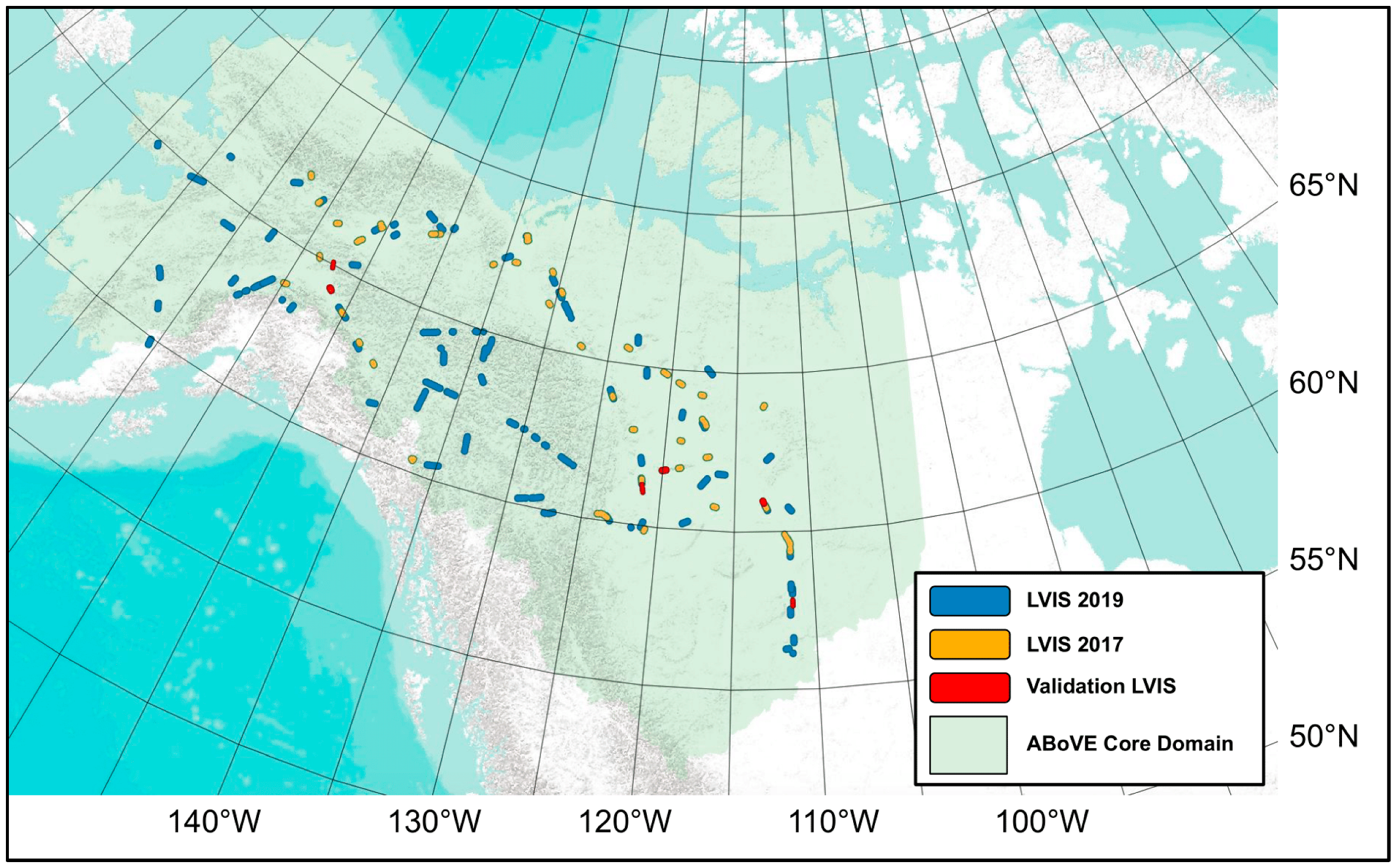
Figure 1. A map of Canada and Alaska showing the locations of the LiDAR flightlines used in this study. The green shading over the base map delineates the Arctic Boreal Vulnerability Experiment (ABoVE) Core Region. Blue and orange flightlines, taken from the 2017 and 2019 airborne LIDAR campaigns, respectively, were included in all analyses and model training. Red flightlines were excluded from any analysis and were used exclusively for validating random forest models.
Remotesensing 16 02577 g001
Figure 2. The ABoVE-LULC PFT composition expressed as a percentage of the total number of PFT observations for the following datasets: the entire ABoVE Domain, every LVIS flightline from 2017 and 2019 in the ABoVE Domain, the LVIS training flightlines used in this study, and the LVIS validation flightlines used in this study.
Remotesensing 16 02577 g002
Figure 3. (a) Box plots of plant height for each original NEON growth form, with legend colors corresponding to the reduced NEON growth groups; (b) the relationship between MCD and plant height, with colors denoting NEON growth groups; (c) the relationship between SD and plant height, with colors denoting NEON growth groups; (d) the relationship between stem diameter and crown height, with colors denoting specific taxa. For plots (ac), the universal relationship is depicted by a black LOESS line and the group-specific relationships are depicted by colored LOESS lines. Gray shading indicates the 95% confidence interval of each LOESS line.
Remotesensing 16 02577 g003
Figure 4. The universal relationship between canopy height and VC is depicted by the black scatter plot and the relationships between canopy height and VC for individual PFTs are depicted by the colored LOESS lines. The gray shading around each LOESS line represents the 95 percent confidence interval. Points with canopy heights near zero but high VCs likely represent LiDAR measurements of wetlands and water that are erroneously classified.
Remotesensing 16 02577 g004
Figure 5. Violin plots and box plots of VC for each PFT. Violin width depicts VC value density while the bottom, middle, and top lines of each white box plot represent the 25th, 50th, and 75th percentiles, respectively.
Remotesensing 16 02577 g005
Figure 6. LiDAR waveforms associated with the ABoVE-LULC (a) coniferous forest class; (b) deciduous forest class; (c) mixed forest class; (d) and woodland forest class. Each PFT class is represented by 100 randomly selected waveforms. Red and blue lines represent the mean and median values from those 100 waveforms, respectively. Violins in the upper right corner of each plot show the distribution of VC values associated with each group of 100 waveforms. Refer to Figure 5 for a comparison of the distributions of VC values in this figure and the distributions of VC values associated with each PFT across the entire ABoVE study domain.
Remotesensing 16 02577 g006
Figure 7. LiDAR waveforms associated with different ranges of VC between (a) 0.0 and 0.2; (b) 0.2 and 0.4; (c) 0.4 and 0.6; (d) and 0.6 and 0.8. Each VC bin is represented by 100 randomly selected waveforms. Red and blue lines represent the mean and median values from those 100 waveforms, respectively. Refer to Figure 4 to compare these waveform structures to the relationship between canopy height and VC.
Remotesensing 16 02577 g007
Figure 8. Relationships of VC to (a) MAT and (b) PRCP. The relationship across all PFTs is depicted by the red LOESS line with gray borders and the black scatter plot. The relationships for individual PFTs are depicted by the colored LOESS lines. Light gray shading around each LOESS line represents the 95 percent confidence interval.
Remotesensing 16 02577 g008
Figure 9. The percentage of each ABoVE-LULC PFT class that is present in the different Köppen–Geiger climate classes and subclasses for every LVIS 2017 and 2019 flightline in the ABoVE Domain.
Remotesensing 16 02577 g009
Figure 10. Relationships between (a) LTSO, (b) LTGSL, (c) ASO, (d) AGSL, and VC. The relationship for all PFTs is depicted by the red LOESS line with gray borders and the black scatter plot. The relationships for individual PFTs are depicted by the colored LOESS lines. Light gray shading around each LOESS line represents the 95 percent confidence interval.
Remotesensing 16 02577 g010
Figure 11. Relationships between (a) SWIR2, (b) NBR, (c) NIR, (d) NDVI, and VC. The relationship for all PFTs is depicted by the red LOESS line with gray borders and the black scatter plot. The relationships for individual PFTs are depicted by the colored LOESS lines. Light gray shading around each LOESS line represents the 95 percent confidence interval.
Remotesensing 16 02577 g011
Figure 12. (a) Variable importance plot for random forest Model C; (b) the relationship between predicted and observed VC for Model C on the sampled validation dataset; (c) the relationship between predicted and observed VC for Model C on the six LVIS flightlines that were reserved from analysis, training, and testing. The red lines in plots (a,b) represent a perfect one-to-one relationship.
Remotesensing 16 02577 g012
Figure 13. (a) A map of Northern Canada and Alaska indicating the location of the HLS tile where random forest Model C was used to predict VC. The HLS tile in (a) overlaps with one of the LVIS 2017 held-out validation flightlines. A closer view of the predicted VC values for the entire HLS tile which borders Great Slave Lake in the Northwest Territories is offered in (b). The observed VC values for the 2017 reserved flightline are depicted in (c) The VC values predicted by Model C are shown in (d). The bright green border in (d) represents the boundary of the LVIS 2017 validation flightline shown in (c).
Remotesensing 16 02577 g013
Table 1. The descriptions, datasets, and units for every variable that was included in the analysis or modeling for this study.
DatasetVariable NameDescriptionUnits
ABoVE-PhenoAnnual spring onset (ABoVE-Pheno ASO)The year-specific date that a pixel achieves half-maximum EVI amplitudeDay of year (DOY)
ABoVE-PhenoLong-term spring onset (LTSO)The multi-year mean of the date that a pixel achieves half-maximum EVI amplitudeDay of year (DOY)
ABoVE-PhenoAnnual autumn onset (ABoVE-Pheno AAO)The year-specific date that a pixel drops below half-maximum EVI amplitudeDay of year (DOY)
ABoVE-PhenoLong-term autumn onset (LTAO)Multi-year mean of the date that a pixel drops below half-maximum EVI amplitudeDay of year (DOY)
ABoVE-PhenomaxEVIAnnual maximum EVI signal
MS-LSPASOThe year-specific date that a pixel achieves 50% EVI amplitudeDay of year (DOY)
MS-LSPAAOThe year-specific date that a pixel drops below 50% EVI amplitudeDay of year (DOY)
MS-LSPOGMxThe year-specific date that a pixel achieves 90% EVI amplitudeDay of year (DOY)
MS-LSPOGMnThe year-specific date that a pixel drops below 90% EVI amplitudeDay of year (DOY)
MS-LSPPeakThe year-specific date that a pixel drops below 10% EVI amplitudeDay of year (DOY)
HLSSWIR1Landsat 8 shortwave infrared band 1
HLSSWIR2Landsat 8 shortwave infrared band 2
HLSNIRLandsat 8 near-infrared band
HLSNBRNormalized burn ratio
HLSNDVINormalized difference vegetation index
DaymetMATAnnual median of maximum daily temperature°C
DaymetMnATAnnual mean of maximum daily temperature°C
DaymetMdMnATAnnual median of minimum daily temperature°C
DaymetAMTAnnual minimum of daily minimum temperature °C
DaymetPRCPTotal annual precipitationmm
Table 2. Table 2 shows the original ABoVE-LULC land cover classes, the PFT groupings created for this study, and their corresponding NEON growth forms. The height ranges that are specified for each land cover in the ABoVE-LULC documentation are included in the rightmost column.
ABoVE-LULC ClassPFT GroupsNEON Growth GroupHeight Range
Coniferous ForestConiferous ForestMature Tree>3 m
Deciduous ForestDeciduous ForestMature Tree>3 m
Mixed ForestMixed ForestMature Tree>3 m
WoodlandWoodlandMature Tree>3 m
Low ShrubShrubShrub Form5–30 cm
Tall ShrubShrubShrub FormBetween 50 cm and 3 m
Open ShrubShrubShrub FormLess than 3 m
HerbaceousHerbaceousn/an/a
Tussock TundraHerbaceousn/an/a
Sparsely VegetatedHerbaceousn/an/a
FenWetlandn/an/a
BogWetlandn/an/a
Shallows/littoraln/an/an/a
Barrenn/an;an/a
Watern/an/an/a
Table 3. Random forest variable configurations. Green cells indicate that a variable was used in the model associated with that column. The number in each cell is the relative importance (RI) of that variable. Variable importance is calculated for each variable by comparing the performance of each decision tree when that variable is permuted and when it is not. The results of these comparisons are averaged for every tree in the random forest and normalized as a percentage of the importance awarded to the most important predictor variable in the model. Therefore, importance represents the performance reduction that occurs when a variable is effectively removed from the model.
Predictor VariableModel AModel BModel CModel D
PFT100%100%100%100%
ASO26.67%26.38%
LTSO48%
AGSL15.40%3.29%
LTGSL46.85% 23.87%
ABoVE-Pheno ASO14.40%
MaxEVI18.17%
OGMx23.59%25.52%20.81%
OGI25.70%5.96%
Peak15.91%16.43%
SWIR110.13%11.22%
SWIR210.80%14.27%2.258%16.23%
NIR 0.00%
Red 0.000%
NBR2.78%5.64%
NDVI
PRCP0.000%0.00% 2.19%
MAT6.73%4.39%4.48%
MnAT13.11%5.62% 7.56%
MdMnAT7.37%4.22%
AMT
Table 4. R-squared, MAE, and RMSE for k-fold, SampVal, and FLVal validation on Random Forest Models. Green cells indicate the model with the highest R-squared for each validation method. Model B had the highest performance on K-fold cross-validation and SampVal. Model C had the worst performance on K-fold cross-validation and SampVal, but the highest performance on FLVal. Model D, which had no phenological predictor variables, had a significantly lower performance on FLVal than Models A, B, and C.
Validation MethodModel AModel BModel CModel D
K-fold cross-validationR2: 0.68
MAE: 0.07
RMSE: 0.09
R2: 0.73
MAE: 0.06
RMSE: 0.08
R2: 0.67
MAE: 0.06
RMSE: 0.08
R2: 0.68
MAE: 0.06
RMSE: 0.09
SampValR2: 0.77
MAE: 0.06
RMSE: 0.07
R2: 0.80
MAE: 0.05
RMSE: 0.07
R2: 0.75
MAE: 0.06
RMSE: 0.08
R2: 0.78
MAE: 0.05
RMSE: 0.08
FLValR2: 0.49
MAE: 0.08
RMSE: 0.10
R2: 0.50
MAE: 0.08
RMSE: 0.10
R2: 0.52
MAE: 0.08
RMSE: 0.10
R2: 0.38
MAE: 0.09
RMSE: 0.11
Disclaimer/Publisher’s Note: The statements, opinions and data contained in all publications are solely those of the individual author(s) and contributor(s) and not of MDPI and/or the editor(s). MDPI and/or the editor(s) disclaim responsibility for any injury to people or property resulting from any ideas, methods, instructions or products referred to in the content.