Direction of Arrival Joint Prediction of Underwater Acoustic Communication Signals Using Faster R-CNN and Frequency–Azimuth Spectrum

Abstract

Utilizing hydrophone arrays for detecting underwater acoustic communication (UWAC) signals leverages spatial information to enhance detection efficiency and expand the perceptual range. This study redefines the task of UWAC signal detection as an object detection problem within the frequency–azimuth (FRAZ) spectrum. Employing Faster R-CNN as a signal detector, the proposed method facilitates the joint prediction of UWAC signals, including estimates of the number of sources, modulation type, frequency band, and direction of arrival (DOA). The proposed method extracts precise frequency and DOA features of the signals without requiring prior knowledge of the number of signals or frequency bands. Instead, it extracts these features jointly during training and applies them to perform joint predictions during testing. Numerical studies demonstrate that the proposed method consistently outperforms existing techniques across all signal-to-noise ratios (SNRs), particularly excelling in low SNRs. It achieves a detection F1 score of 0.96 at an SNR of −15 dB. We further verified its performance under varying modulation types, numbers of sources, grating lobe interference, strong signal interference, and array structure parameters. Furthermore, the practicality and robustness of our approach were evaluated in lake-based UWAC experiments, and the model trained solely on simulated signals performed competitively in the trials.

1. Introduction

Detecting and recognizing underwater acoustic communication (UWAC) signals is a crucial and challenging task, with applications ranging from civilian to military domains, such as underwater resource exploration, navigation and positioning, maritime security and defense, marine ecological monitoring, and the establishment of underwater communication networks [1,2]. Accurate and efficient identification of underwater acoustic signals is paramount yet challenging, particularly in scenarios with low signal-to-noise ratios (SNRs) and complex UWAC channels. This challenge arises because of the significant propagation loss and intricate multipath effects in UWAC channels. Hydrophone arrays and precise beamforming algorithms partially address these challenges by leveraging time, frequency, and spatial information. These techniques enhance the SNR and enable the effective separation of signals originating from different azimuths, even when these signals overlap in the time and frequency domains. In this study, we propose a novel joint prediction method using the frequency–azimuth (FRAZ) spectrum [3] of array signals and a faster region-based convolutional neural network (Faster R-CNN) [4]. This approach further addresses the aforementioned challenges and enables the joint prediction of UWAC signal information, including the number of sources, modulation type, frequency band, and direction of arrival (DOA).

Traditional methods cannot effectively address these challenges because they typically treat DOA estimation, signal detection, and recognition as separate tasks. This makes processing an indeterminate number of UWAC signal targets with overlapping time and frequency domains difficult [5]. By contrast, these signals can often be distinguished using spatial-domain DOA estimation algorithms. Conventional beamforming (CBF) [6] is the most popular DOA estimator in practice because of its robustness. However, the array gain and angular resolution of CBF are low, limiting the signal-capturing capability and precision of DOA estimation. High angular resolutions and array gains are achievable using other methods, albeit with lower robustness. Techniques such as multiple signal classification (MUSIC) [7] and other subspace-based DOA estimation methods [8,9] aim to orthogonalize signal and noise subspaces; however, they rely heavily on the precise estimation of the number of sources and are ineffective in low-SNR environments. An alternative is the minimum-variance distortionless response (MVDR) [10], a type of data-adaptive algorithm [11,12], which uses the statistical properties of the received signals to directly optimize the array weights, suppressing interference and improving SNR. However, these algorithms are sensitive to statistical mismatches such as inaccuracies in the covariance matrix estimation and deviations in the statistical distributions of the signals and noise, degrading performance in non-ideal conditions.

Recent studies have developed data-driven signal DOA estimation methods based on deep learning. In these studies, the task of signal DOA estimation has been modeled as on-grid classification [13,14,15,16,17,18,19,20,21] or off-grid regression [21,22,23,24,25] and has been performed using deep neural networks. In particular, multisource DOA estimation has evolved into a multilabel prediction problem [18,19,20,21]. Multi-layer perceptrons [14,16], convolutional neural networks (CNNs) [13,15,18,19,20,21,24,25], recurrent neural networks [22,23], Transformers [17], and their combinations are now widely used to extract signal features. The inputs of these models are typically the raw array signal [15,21,23], spatial covariance matrix [13,14,16,17,19,22,25,26], or beam of the array signal [20]. Building on this body of work, our approach transforms the UWAC DOA estimation task and other joint prediction tasks into an object detection framework within a FRAZ spectrum, offering a novel perspective on multisource broadband signal processing.

Recent studies have extended signal joint prediction tasks to include not only detection and recognition but also frequency band estimation. References [27,28,29,30] jointly predict communication signals using deep-learning object detection algorithms on single-channel signal spectrograms. Joint prediction in microphone array signal processing has also been investigated using sound-event localization and detection (SELD) algorithms [31]. SELD predicts multiple DOAs and associates each with a specific sound event type over time. Inputs for SELD algorithms typically include spectrograms or Mel spectrograms [31,32,33,34,35,36], raw waveforms [37,38,39], steered response power with phase transform (SRP-PHAT) [40,41], and generalized cross-correlation with phase transform (GCC-PHAT) [42,43,44,45]. These inputs implicitly represent the azimuth and type of the target sources, and they are processed through high-dimensional deep neural networks to obtain accurate maps. However, to avoid the complexity and non-intuitive mapping obtained using these input features, our study uses the FRAZ spectrum to obtain a more intuitive and robust method for extracting joint prediction features.

The energy distribution of a UWAC signal on a FRAZ spectrum is visible as a thick horizontal strip (Figure 1a–c). The position of the strip along the azimuthal axis indicates the DOA, whereas its placement along the frequency axis denotes the signal frequency band. Here, the carrier frequency aligns precisely with the center of the strip. Note that these strips are not uniformly narrow. They tend to widen in the low-frequency range because of the widening of the main lobe of the signal. This specific energy distribution pattern enables object detection methods to detect and localize these strips on the FRAZ spectrum, which facilitates the estimation of signal frequency band and DOA.

Figure 1. FRAZ and spatial spectra of seven UWAC signals. (a) CBF FRAZ spectrum. (b) MVDR FRAZ spectrum. (c) MUSIC FRAZ spectrum. (d) CBF spatial spectrum. (e) MVDR spatial spectrum. (f) MUSIC spatial spectrum.

A FRAZ spectrum also encapsulates the spectral features of the signal. As shown in Figure 1a–c, variations in strip shape correspond to different UWAC signal modulation formats, enabling their recognition. In this study, Faster R-CNN jointly predicts signals by detecting and analyzing the strips on the FRAZ spectrum, thereby enhancing both its precision and efficiency.

In contrast to traditional approaches, which typically involve postprocessing the energy accumulation across all frequencies, the proposed method leverages the spatial and frequency spectrum features of the UWAC signal to significantly improve broadband DOA estimation. Our method hence has three advantages over traditional methods. First, it effectively estimates the DOAs of broadband signals for varying numbers of sources and frequency bands while facilitating the joint prediction of additional UWAC signal parameters. As illustrated in Figure 1a–c, after the signals have been detected by bounding boxes, their frequency band range, DOA, and modulation type can be determined. Furthermore, the number of signal sources can be deduced from the number of bounding boxes. This approach streamlines the process and enhances the accuracy of DOA and signal characterization.

Second, the proposed method performs better under strong interference. Traditional methods tend to smooth out weaker signals during postprocessing over frequency bands. In contrast, our method concentrates on the specific frequency bands where the UWAC signal power is distributed, preserving the integrity of weak signal features. Signals 3 and 4 exhibit weak energy features in the FRAZ spectra (Figure 1a–c), but they are smoothed out in the spatial spectra (Figure 1d–f). Furthermore, our method distinguishes UWAC signals with weak energies from interference or stronger signals located in different frequency bands. The main energy peaks of signal 7 primarily stem from low-frequency interference (Figure 1d–f), leading to false detections or misses. However, because our method considers only the relevant frequency band and prevents the accumulation of energy across the spectrum, it detects weaker signals, significantly reducing the likelihood of false detections or misses.

Finally, the proposed method effectively mitigates the interference caused by grating lobes in DOA estimation. The physical size of a hydrophone and structural design of an array typically constrain the central frequency, which, when exceeded by the frequency of the UWAC signal, results in grating lobes. These lobes often mimic actual UWAC signals, leading to potential false peaks in the spatial spectrum and increasing the likelihood of erroneous detections (Figure 1d). However, in a FRAZ spectrum, the characteristics of the grating lobes are markedly different from those of genuine signals; grating lobes manifest as curved forms, whereas true signals appear as distinct strips. This unique morphology in the FRAZ spectrum enables us to accurately distinguish true signals from grating lobe interference.

Deep-learning-based algorithms [19,21] for DOA estimation address several challenges inherent to traditional methods, particularly in scenarios with low SNRs. However, they typically require extensive training data and rely on the assumption that both training and test data are independently and identically distributed (i.i.d.). This dependence limits their flexibility, hindering accurate estimation of the DOA for an arbitrary number of sources or adaption when faced with changes in noise distribution and array structure parameters. Crucially, these methods must be trained on a wide range of signal distributions that include all SNRs and DOA angle distributions [19].

The proposed method based on FRAZ spectrum and Faster R-CNN is designed to overcome these limitations. In contrast to spatial covariance matrices or raw signal analysis, the FRAZ spectrum provides a robust characterization across various signal source counts and array structure parameters. Additionally, Faster R-CNN, a two-stage object detection method, has an architecture that gives it good generalization abilities and robustness against interference in UWAC. The first stage of Faster R-CNN is dedicated to high-efficiency signal detection, while the second stage concentrates on precise signal modulation recognition and parameter estimation, leveraging both the detection results and detected signal features. Thus, the use of two-stage Faster R-CNN enables our approach to accurately detect an arbitrary number of signal targets within a specific frequency band, effectively minimizing noise and interference. Crucially, this approach requires considerably less training data and exhibits superior generalization capabilities.

In this study, we developed a joint prediction method for UWAC signals. This method integrates signal detection, modulation recognition, frequency band estimation, and broadband DOA estimation for complex UWAC channels. Employing FRAZ spectra as input and Faster R-CNN as the detection framework, our approach detects, localizes, and recognizes signals across the two-dimensional frequency–azimuth domain. The primary contributions of this study are as follows.

(1)

Joint Prediction Capability: The proposed framework for UWAC signals simultaneously determines the number of sources, recognizes modulation types, estimates frequency bands, and computes DOAs. This integrated approach enhances the efficiency and accuracy of signal processing in complex acoustic environments.

(2)

Application of FRAZ Spectrum and Faster R-CNN: This approach has strong generalization ability and can predict an arbitrary number of sources. It also extends the detection frequency range of the hydrophone array without interference from grating lobes.

(3)

Empirical Evaluation: Numerical studies were conducted to evaluate the effectiveness of our method in both simulated and experimental scenarios. The model trained solely on the simulated data performed competitively when applied to actual experimental data.

The remainder of this paper is structured as follows: Section 2 presents the signal model and FRAZ spectrum. Section 3 describes the Faster R-CNN model for joint prediction. Section 4 and Section 5 cover the simulation and experimental studies, respectively. Finally, our conclusions are presented in Section 6.

2. Signal Model

2.1. UWAC Signal

UWAC systems use many modulation formats and parameters to accommodate diverse application scenarios, which vary with factors such as communication distance and rate. Common modulation formats in UWAC include multiple frequency shift keying (MFSK), multiple phase shift keying (MPSK), linear frequency modulation (LFM), and orthogonal frequency division multiplexing (OFDM).

The received modulated UWAC signal can be expressed as follows:

$$\phi (t)=s(t)\otimes h(t)+n(t),$$

(1)

where $s(t)$ is the transmitted modulated signal, $h(t)$ is the UWAC response, $n(t)$ is ambient noise, and $\otimes$ is the convolution operator.

When the transmitted signal undergoes modulation via MFSK, $s(t)$ can be expressed as follows:

$$s{(t)}_{\mathrm{MFSK}}=A{e}^{j(2\pi f_{c}t+\theta )}{\displaystyle \sum _{l=-\infty }^{\infty }{e}^{j2\pi f_{\Delta }\left(s_{l}t-l{T}_0\right)}\delta (t-l{T}_0)},$$

(2)

where $A$, $f_c$, $\theta$, $f_{\Delta }$, and $T_0$ denote the amplitude, carrier frequency, initial phase, frequency deviation, and symbol rate, respectively, and $s_l$ denotes the $l$ period. $\delta (t-l{T}_0)$ can be expressed as follows:

$$\delta (t-l{T}_0)=\left\{\begin{array}{c}1,(l-1)T_0\le \left|t\right|\le l{T}_0\\ 0, otherwise\end{array}\right..$$

(3)

When the transmitted signal undergoes modulation via MPSK, $s(t)$ can be expressed as follows:

$$s{(t)}_{\mathrm{MPSK}}=A{e}^{j(2\pi f_{c}t+\theta )}{\displaystyle \sum _{l=-\infty }^{\infty }{b}_l\delta (t-l{T}_0)},$$

(4)

where $b_l$ is the symbol in one period and is assigned the value of $\cos (2\pi (m-1)/M)$. $M$ represents the modulation order of the MPSK signal, and $m$ (ranging from $0$ to $M-1$) constitutes the symbol set.

When the transmitted signal undergoes modulation via OFDM with BPSK subcarrier modulation, $s(t)$ is expressed as follows:

$$s{(t)}_{OFDM}=A{e}^{j(2\pi f_{c}t+\theta )}{\displaystyle \sum _{k=0}^{K-1}{\displaystyle \sum _{l=-\infty }^{\infty }{b}_{k,l}{e}^{j2\pi k\Delta f(t-l{T}_b)}\delta (t-l{T}_b)}},$$

(5)

where $K$ and $T_b$ are the number of subcarriers and OFDM symbol rate, respectively, $\Delta f$ is the subcarrier bandwidth of OFDM, and $b_{k,l}$ is the $lth$ symbol in the $kth$ subcarrier.

When the transmitted signal is LFM, $s(t)$ can be expressed as follows:

$$s{(t)}_{LFM}=A{e}^{j(2\pi f_{0}t+\pi k_0{t}^2)},$$

(6)

where $f_0$ and $k_0$ are the start frequency and chirp rate, respectively.

2.2. UWAC Signal

As shown in Figure 2, for a uniform linear array (ULA) with $M$ hydrophone elements and an element interval of $d$, its two-dimensional space-time response can be written as

$$\psi [d,t]=A\phi (t)+n(t),$$

(7)

where $d={[0,{\mathbf{d}}_1,{\mathbf{d}}_2,\cdots {\mathbf{d}}_{M-1}]}^T$ is the spatial position of the element, $t$ is the sample time, $n(t)$ is Gaussian white noise that is i.i.d. and independent of the signals, $\phi (t)={[{\phi }_1(t),{\phi }_2(t),\cdots ,{\phi }_L(t)]}^T$ is $L$ uncorrelated UWAC sources, and $A$ is an array manifold vectors.

$$A=\left[a\left({\kappa }_1\right),a\left({\kappa }_2\right),\cdots ,a\left({\kappa }_L\right)\right],$$

(8)

where $a({\kappa }_i)=[1,e^{j2\pi f{\kappa }_i\cdot d_1/c},\cdots ,e^{j2\pi f{\kappa }_i\cdot d_{M-1}/c}]$, ${\kappa }_i$ is the unit direction vector of the $i$-th UWAC source, $f$ is the frequency of the UWAC signal, and $c$ is the speed of sound. Specifically, the frequency spectrum response received by the $m$-th element of the ULA from an incident signal at the azimuth angle $\theta$ is as follows:

$$\psi [m,f]=\frac{1}{T}{\displaystyle \sum _{t=0}^{T-1}(\phi (t)e^{j2\pi fmd\sin \theta /c}+n_m(t))}{e}^{-j2\pi ft/T}.$$

(9)

Figure 2. Uniform linear array signal model.

Then, the FRAZ spectrum can be defined as follows:

$$\begin{array}{c}\psi [\widehat{\theta },f]=\frac{1}{MT}{\displaystyle \sum _{m=1}^M{\displaystyle \sum _{t=0}^{T-1}[}}\phi (t)e^{j2\pi fmd\sin \theta /c}\\ +n_m(t)]e^{-j2\pi ft/T}{e}^{-j2\pi fmd\sin \widehat{\theta }/c}\end{array},$$

(10)

where $\widehat{\theta }$ denotes directional scanning in the beamforming domain. Equation (10) shows that the FRAZ spectrum achieves its peak energy when the scanning angle aligns with the actual DOA of the UWAC signal. The FRAZ spectrum encapsulates the UWAC signal frequency and azimuth spectrum features of the incoming signal. Hence, joint prediction can be achieved by extracting the energy distribution features in the FRAZ spectrum.

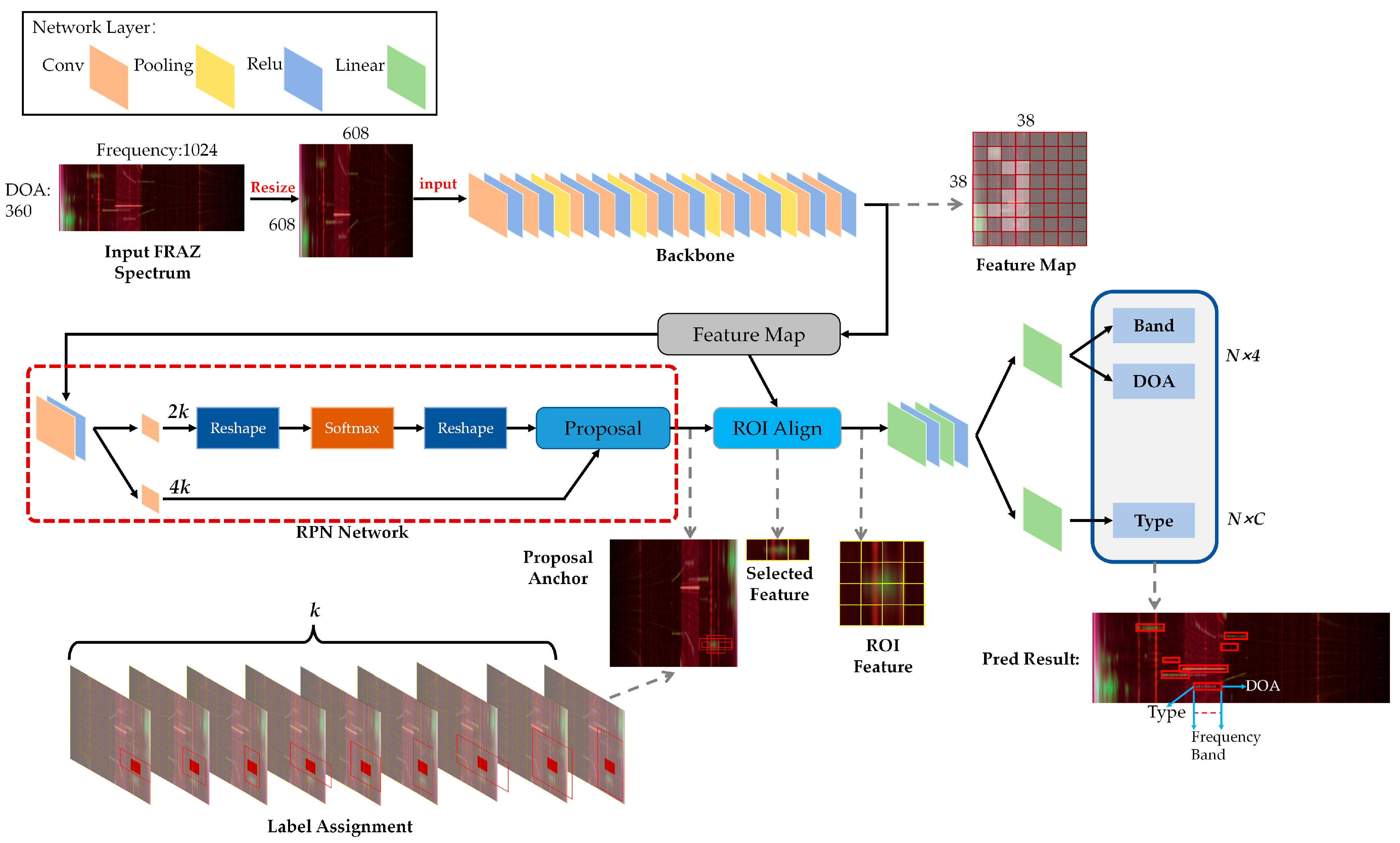
3. Faster R-CNN for Joint Prediction

Using the FRAZ spectrum, Faster R-CNN performs joint predictions by estimating the bounding box once it has detected a signal. The parameters of the bounding boxes encapsulate multiple aspects of the signal: the position along the frequency axis determines the frequency band, its azimuth position indicates the DOA, the category of a bounding box anchor identifies the modulation type, and the number of bounding boxes indicates the number of signals present.

As depicted in Figure 3, initially, the UWAC signals are transformed into a FRAZ spectrum and the spectrum image is resized to optimize feature extraction. The backbone network extracts the azimuth and frequency features, yielding a feature map with a downsampling factor of 16. This feature map is then fed into the region proposal network (RPN) to predict the proposed anchor. Features within these anchors are subsequently extracted and processed by the region of interest (RoI) alignment module to perform feature warping. Finally, these features undergo joint prediction in the classification and regression subnetworks. The regression subnetwork determines the frequency band and DOA, whereas the classification subnetwork recognizes the signal modulation.

Figure 3. General architecture of Faster R-CNN using a FRAZ spectrum as input for UWAC signal joint prediction.

3.1. Input FRAZ Spectrum and Feature Extraction

In DOA estimation research, the CBF algorithm is renowned for its robustness, whereas adaptive algorithms such as MVDR perform well under strong interference. Additionally, the MUSIC algorithm has exceptional angular resolution and gain. To harness the strengths of each algorithm, we propose a combination of the FRAZ spectrum from all three algorithms to form a composite input analogous to an RGB image in natural imaging systems (Figure 4). Specifically, the FRAZ spectrum from the CBF algorithm $\psi {[\theta ,f]}_{CBF}$, MVDR algorithm $\psi {[\theta ,f]}_{MVDR}$, and MUSIC algorithm $\psi {[\theta ,f]}_{MUSIC}$ are assigned to the three channels of an RGB image format. This tri-channel FRAZ spectrum, expressed as follows, is the input to our model:

$$\psi [\theta ,f,3]=\left\{\psi {[\theta ,f]}_{CBF};\psi {[\theta ,f]}_{MUSIC};\psi {[\theta ,f]}_{MVDR}\right\}.$$

(11)

Figure 4. Input feature combination.

To ensure compatibility with the model and enhance its adaptability, the input FRAZ spectrum is resized to fixed dimensions before processing. This resizing is essential not only to accommodate variations in array structures and transformation parameters of FRAZ spectrum but also to maintain a balance in feature extraction across both the frequency and azimuth domains. Using a standard input size enables the model to better learn and generalize across different conditions, thereby improving its signal-prediction accuracy and robustness.

To effectively extract the UWAC signal features from a FRAZ spectrum, a deep CNN is employed as the backbone network to capitalize on the nonlinear fitting ability of its expanded receptive field. First, the input FRAZ spectrum of size $W_f^{input}\times H_{\theta }^{input}$ is resized to $W_f^{resize}\times H_{\theta }^{resize}=608\times 608$. It is then passed through the backbone network for feature extraction with a downsampling rate $M=16$, resulting in a feature map of size $W_f^{out}\times H_{\theta }^{out}=38\times 38$. Each feature mapping point represents signal characteristics within a specific frequency and azimuth range. For instance, consider a signal with a sampling rate of $f_s=64,000$, DOA search number of ${\theta }_{range}=180$, and DOA resolution of $\Delta \theta =0.5°$, implying a DOA search range of $[-90°,90°]$. The feature mapping point $F_{i,j}$ at position $(i,j)$ encapsulates signal frequencies ranging from $f_{low}$ to $f_{high}$, calculated as follows:

$$f_{low}=\frac{(i-1)\times f_s\times M}{2W_f^{resize}},$$

(12)

$$f_{high}=\frac{i\times f_s\times M}{2W_f^{resize}}.$$

(13)

That is, the lower and higher frequency boundaries of a feature map point are $f_{low}\approx (i-1)\times 842$ Hz and $f_{high}\approx i\times 842$ Hz, indicating that a mapping point contains a frequency feature of approximately 842 Hz. Similarly, the mapping point covers the DOA range from ${\theta }_{low}$ to ${\theta }_{high}$, where

$${\theta }_{low}=\frac{(j-H_{\theta }^{out}/2-1)\times {\theta }_{range}\times M}{\Delta \theta \times H_{\theta }^{resize}},$$

(14)

$${\theta }_{high}=\frac{(j-H_{\theta }^{out}/2)\times {\theta }_{range}\times M}{\Delta \theta \times H_{\theta }^{resize}}.$$

(15)

Therefore, the lower and higher DOA boundaries are ${\theta }_{low}\approx (j-20)\times 4.737°$ and ${\theta }_{high}\approx (j-19)\times 4.737°$, yielding an azimuth feature of approximately 4.737° at this mapping point. For each mapping point, these features are sent to the RPN for the region proposal stage, facilitating the two-dimensional search for signals across the frequency–azimuth domain.

3.2. Signal RPNs

The proposal of signal regions involves a targeted search for UWAC signals within a predefined region in the two-dimensional FRAZ spectrum across both frequency and azimuth axes. When a potential signal target is detected, an anchor box corresponding to the designated area is predicted. The number of anchor boxes should be clearly defined prior to executing the RPN computations to improve signal region proposal accuracy and efficiency, optimizing the overall signal detection performance of the network.

As illustrated in Figure 3, each feature mapping point is defined as the frequency and azimuth center of the signal, and it encompasses the frequency range and azimuth of the signal, as detailed in Equations (13)–(15). The RPN operates by detecting signals at the central points. Because of the broad ranges of frequencies and azimuths in each feature map, a single center point may represent multiple signals. Moreover, variations in signal frequency bands and the DOA main-lobe widths necessitate the use of various anchor box sizes.

We configured different regions within the feature map to represent distinct frequency bandwidths and main-lobe widths, each corresponding to a unique anchor box size. As shown in Figure 3, we set up $k$ regions with different sizes. For instance, for the example signal described in Section III-A, we assume the length of the Fourier transform to be $N_{FFT}=2048$ and that the dimension of the input FRAZ spectrum is $W_f^{input}\times H_{\theta }^{input}=1024\times 360$. We consider carrier frequencies from $f_{low}^c=5000$ Hz to $f_{high}^c=15,000$ Hz, and bandwidths from $B_{low}=2000$ Hz to $B_{high}=5000$ Hz. Given the high frequency characteristics typical of a UWAC signal, the DOA main-lobe width is generally narrow, leading us to set all the anchor box heights to $h_{anchor}=6$ pixels (3°). The width of the anchor box is determined to ensure coverage across all potential signal frequency bands. That is, the $i$th anchor box width at pixel $w_{anchor}^i$ is set as follows:

$$\begin{array}{c}{w}_{anchor}^i={\lambda }_{low}{B}_{low}\times \frac{2W_f^{input}}{f_s}\\ +\frac{[({\lambda }_{high}{B}_{high}-{\lambda }_{low}{B}_{low})\times (i-1)]}{(k-1)}\times \frac{2W_f^{input}}{f_s}\end{array}.$$

(16)

Here, ${\lambda }_{low}=0.8$ and ${\lambda }_{high}=1.2$ serve as the bandwidth adjustment coefficients. These coefficients increase the frequency band range, ensuring that the resultant anchor box encompasses all potential signals. Hence, the $i$th anchor box width is $w_{anchor}^i=51.2+17.6\times (i-1)$ pixels, effectively covering the extended frequency range.

After the anchor box proposals have been generated, bounding box regression is applied to refine the position and size of the anchor box, thereby obtaining precise estimates of the DOA and frequency band. The regression process uses four coordinates, defined as follows:

$$\left\{\begin{array}{ll}{t}_{\mathrm{x}}=\left(x-x_{anchor}\right)/w_{anchor},& t_{\mathrm{y}}=\left(y-y_{anchor}\right)/h_{anchor},\\ t_{\mathrm{w}}=\log \left(w/w_{anchor}\right),& t_{\mathrm{h}}=\log \left(h/h_{anchor}\right),\\ t_{\mathrm{x}}^{\ast }=\left(x^{\ast }-x_{anchor}\right)/w_{anchor},& t_{\mathrm{y}}^{\ast }=\left(y^{\ast }-y_{anchor}\right)/h_{anchor},\\ t_{\mathrm{w}}^{\ast }=\log \left(w^{\ast }/w_{anchor}\right),& t_{\mathrm{h}}^{\ast }=\log \left(h^{\ast }/h_{anchor}\right),\end{array}\right.$$

(17)

where $x_{anchor}$ and $y_{anchor}$ represent the center coordinates of the anchor, while $w_{anchor}$ and $h_{anchor}$ denote its width and height, respectively. Variables $x$, $x_{anchor}$, and $x^{\ast }$ are the predicted anchor, and true boxes, respectively (likewise for $y$, $w$, and $h$). The four coordinates encapsulate both the DOA and frequency band information of the detected signal. As depicted in the RPN in Figure 3, two feature maps with channel dimensions of $2k$ and $4k$ are output after a convolution block. The $2k$-channel feature map is employed for binary classification to detect a UWAC signal within the proposed anchor box. The $4k$-channel feature map is used to predict the four coordinates of the anchor box. In each execution of the RPN, $W_f^{out}\times H_{\theta }^{out}\times k$ binary classifications are required for signal detection and box regression. Given that $k$ anchor boxes have been predefined, multiple anchor boxes may overlap with the same signal. Hence, regions where the intersection over union (IoU) exceeds a predetermined threshold are considered positive samples, whereas those with an IoU below this threshold are considered negative samples. During the prediction phase, the non-maximum suppression algorithm [46] is used to identify the correctly predicted anchor boxes, ensuring signal localization accuracy and efficiency.

3.3. Signal RoI Alignment

After the signal detection and preliminary estimation of the DOA and frequency bands using the RPN, Faster R-CNN refines these predictions and recognizes the modulation type of the signal. It does this by extracting signal features from the corresponding DOAs and frequency bands detected by the RPN. Because the sizes of the proposal features vary with the modulation parameters of the UWAC signal, a network with fixed parameters cannot effectively process them. To address this challenge, RoI Align [47] normalizes the features to a consistent size first (see Figure 3).

The RoI Align layer employs maximum pooling to convert the signal RoI features into a fixed-size feature map. This layer then uses bilinear interpolation [48] to ensure precise alignment of feature points within the RoI with their corresponding angular and frequency positions in the original FRAZ spectrum. This alignment enables more accurate extraction of signal feature information from the RoI. A critical advantage of RoI Align is its ability to minimize the loss of the original FRAZ spectrum information in the feature map, enhancing the accuracy and reliability of target detection.

3.4. Signal Joint Prediction Network

After processing through RoI Align, all potential signal targets identified by the RPN network are standardized into a uniform-sized feature map. This map is then flattened and passed through linear classification and regression layers designed for multitask prediction. The linear classification network determines the presence of a signal and recognizes its modulation type. Simultaneously, the linear regression network refines the predictions of the frequency band and DOA of the signal. As shown in Figure 3, the output dimension of the regression network is $N\times 4$ and the output dimension of the classification network is $N\times C$, where ‘$4$’ represents the four coordinates of the bounding box, ‘$N$’ is the number of proposal bounding boxes and ‘$C$’ is the number of modulation types. After the joint prediction phase, the predicted bounding boxes represent the final signal parameters (Figure 3).

For these boxes, the carrier frequency $f_c$ and DOA $\theta$ are defined as follows:

$$f_c=\frac{(w_{start}+w_{end})\times f_s}{4W_f^{input}},$$

(18)

$$\theta =\frac{(h_{start}+h_{end}-H_{\theta }^{input}/2-1)\times \Delta \theta \times {\theta }_{range}}{2H_{\theta }^{input}},$$

(19)

where $(w_{start},h_{start})$ and $(w_{end},h_{end})$ denote the coordinates of top-left and right-bottom corners of the bounding box, respectively. The frequency bandwidth of the UWAC signal is defined by the width of the bounding box.

3.5. Loss Function of Joint Prediction

An end-to-end training approach is employed for Faster R-CNN that enables the RPN and the signal joint prediction network to be simultaneously trained. Consequently, the network loss function is divided into two primary components: the RPN and joint prediction network losses. Specifically, the RPN loss comprises the signal detection and preliminary positioning losses as follows:

$$\begin{array}{c}L(\left\{p_i\right\},\left\{t_i\right\})=\frac{1}{N_{cls}}{\displaystyle \sum _i{L}_{cls}(p_i,p_i^{\ast })}\\ +\lambda \frac{1}{N_{reg}}{\displaystyle \sum _i{p}_i^{\ast }{L}_{reg}(t_i,t_i^{\ast })}\end{array},$$

(20)

where $i$ is the index of all selected positive and negative anchors, and $p_i$ and $p_i^{\ast }$ are the detection result and true label, respectively. Here, $p_i^{\ast }=1$ indicates a positive anchor, and $p_i^{\ast }=0$ indicates a negative anchor. Moreover, $t_i$ is the joint DOA and frequency band estimation result, and $t_i^{*}$ is the true label of DOA and frequency band estimation result; $N_{cls}$ and $N_{reg}$ are normalization coefficients determined by the number of anchors; $L_{cls}(\cdot )$ and $L_{reg}(\cdot )$ are the binary cross-entropy loss and smooth L1 loss, respectively. Finally, $\lambda$ is a weight parameter, as anchor box regression is only performed on positive samples.

The loss function for the joint prediction network is composed of two elements: the signal modulation recognition and precise positioning losses, as follows:

$$L(p,t)=L_{cls}(p,p^{*})+\lambda [p^{*}\ge 1]L_{reg}(t,t^{*}).$$

(21)

Here, $p$ and $p^{*}$ are the recognition result and true modulation type, respectively; $t$ is the precise DOA and frequency band estimation result; and $t^{*}$ is the true label of the DOA and frequency band estimation result. Here, $[p^{*}\ge 1]$ indicates that the loss for class 0 (background) is not calculated, and hence a balancing parameter $\lambda$ is required.

4. Simulation Studies

We employed the results of simulations to evaluate the joint prediction capabilities of the proposed method. Initially, we assessed the performance of the method across varying SNRs, number of sources, and modulation types, including scenarios with the presence of grating lobes. Subsequently, we investigated the robustness of the joint prediction mechanism under varying signal interference levels and hydrophone array parameters.

4.1. Data Generation, Baseline, Training Details, and Metrics

4.1.1. Data Generation

For the training phase, a ULA comprising 32 hydrophone elements was modeled, with each element spaced at 0.075 m intervals. The array operated at a sampling rate of 64,000 Hz. Given a sound speed of 1500 m/s, the center frequency of the array for detection was 10,000 Hz. Detailed specifications of the UWAC source signal are provided in Table 1. All parameters were uniformly distributed within their respective ranges. We considered six common UWAC modulation formats: 2FSK, 4FSK, 8FSK, BPSK, LFM, and OFDM, summarizing the typical ranges of their modulation parameters. Due to the array’s center frequency of 10,000 Hz, the carrier frequency for the training set of UWAC signals was set to not exceed this limit. However, instances where signal frequencies surpass this boundary may induce grating lobe interference, a significant concern in array signal processing. To evaluate the model’s resilience to such interference, test set II was specifically designed. Additionally, the selection of DOA and SNRs was based on conditions typically encountered in UWAC applications. Furthermore, to avoid the impact of excessively high energy differences on detection capabilities, the parameter design strategically limited the SNR differential to 20 dB, as determined through empirical evaluations. But sometimes this happens, so we set up test set III to verify the performance of the models under varying signal interference levels. The hydrophone array was capable of receiving one to seven UWAC signals at a time, across various modulation formats, modulation parameters, and DOAs. The SNRs of these received signals varied significantly, and they often originated from similar DOA and frequency ranges, presenting substantial challenges for accurate signal detection and estimation.

Table 1. Details of Parameters in the Dataset.

Parameter	Training Set	Test Set I	Test Set II	Test Set III	Test Set IV
Number of Signals	4000	6000	6000	6000	8000
DOA Range	−85° to 85°	−85° to 85°	−85° to 85°	−85° to 85°	−85° to 85°
Carrier Frequency (Hz)	5000–8000	5000–8000	5000–15,000	5000–8000	5000–8000
Bandwidth (Hz)	1000–5000	1000–5000	1000–5000	1000–5000	1000–5000
SNR (dB)	−20 to 20	−20 to 20	−20 to 20	30; −20 to 20	−20 to 20
Maximum SNR Difference 1 (dB)	20	20	20	40	40
Number of Sources	1–7	1–7	1–7	2–7	1–7
Number of Array Elements	32	32	32	32	8–64

¹ Maximal SNR Difference refers to the disparity between the signal with the highest and lowest SNR encountered during the signal generation process. In Test Set III, one signal has an SNR of 30 dB, whereas the SNRs of the remaining signals were generated randomly.

4.1.2. Baseline Methods

The MVDR and MUSIC algorithms were employed as benchmarks to assess the DOA estimation and signal detection performance. These algorithms detect signals using a spatial spectrum and peak search algorithm. Specifically, MUSIC employs the minimum description length criterion [49] to determine the number of signal sources. A variation called MUSIC-Known, which operates with a predefined number of signals, was also compared. Because it was given prior information, MUSIC-Known was expected to yield better detection performance. Additionally, we compared a deep-learning-based method. Because DOA estimation for UWAC signals involves broadband estimation tasks, narrowband methods are inappropriate. Consequently, BEAM-CNN, which integrates local signal beams with a CNN [22], was used.

4.1.3. Training Details

In the experiments, we configured the input data snapshot length of these methods at 2048, with the number of snapshots set to 32. To generate the FRAZ spectrum, a Fourier transform of length 2048 was employed, and the angular scanning resolution was set to 0.5°, resulting in a FRAZ spectrum of specified dimensions: $1024\times 360$. The training dataset comprised 4000 FRAZ spectrum samples, featuring a random number of sources ranging from one to seven. We used ResNet50 [50] as the backbone for the Faster R-CNN and optimized it via the SGD optimizer with a learning rate of 10⁻³. The model was trained with a batch size of 1 across 60 epochs to ensure convergence. Further Faster R-CNN parameter settings are documented in [4]. The test set details for various scenarios are presented in Table 1. During the test phase, the model operated at 70.1 frames per second. All experiments were conducted on an Nvidia 4090 GPU using the PyTorch 2.1 deep learning framework.

4.1.4. Metrics

To assess the joint prediction capabilities of the proposed method, we evaluated the performance of the model for detection, DOA estimation, recognition, and frequency-band estimation. The detection F1 score quantifies the detection efficacy of a model. A detection is defined as a true positive when the predicted DOA deviates by no more than 3° from the true DOA. The detection F1 score is defined as follows:

$$F_1=2\times \frac{precision\times recall}{precision+recall}=\frac{2\times TP}{2\times TP+FP+FN},$$

(22)

where precision is calculated as $TP/(TP+FP)$ and recall is $TP/(TP+FN)$, where $TP$, $TN$, $FP$, and $FN$ represent the numbers of true positives, true negatives, false positives, and false negatives, respectively. This metric comprehensively assesses detection performance by balancing the trade-off between precision and recall.

Recognition accuracy was used to evaluate the signal modulation recognition performance. Only when the signal is correctly detected and its modulation format is correctly identified can a sample be called a correct identification (true positive). Recognition accuracy is defined as follows:

$$Accuracy=\frac{TP+TN}{TP+TN+FP+FN}.$$

(23)

The accuracy of the DOA and frequency band estimations was quantified using the mean absolute error (MAE), and it was calculated only for signals that were correctly detected. The MAE for DOA estimation is defined as follows:

$${\epsilon }_{\theta }=E\left[\frac{1}{K}{\displaystyle \sum _{k=1}^K\left|{\theta }_k-{\widehat{\theta }}_k\right|}\right],$$

(24)

where $E(\cdot )$ is the estimated expectation for all signal samples, $K$ is the total number of sources in an input-signal sample, and ${\theta }_k$ and ${\widehat{\theta }}_k$ are the true and estimated DOA of the $k$th signal, respectively. The MAE of the frequency band estimation is defined as follows:

$${\epsilon }_f=E\left[\frac{1}{2K}{\displaystyle \sum _{k=1}^K\left(\left|f_k^{low}-{\widehat{f}}_k^{low}\right|+\left|f_k^{high}-{\widehat{f}}_k^{high}\right|\right)}\right],$$

(25)

where $f_k^{low}$ and ${\widehat{f}}_k^{low}$ are the true and estimated low frequencies of the $k$th signal, respectively. Similarly, $f_k^{high}$ and ${\widehat{f}}_k^{high}$ are the true and estimated high frequencies of the $k$th signal. This approach enabled an objective assessment of the precision of the model in DOA and frequency range estimation.

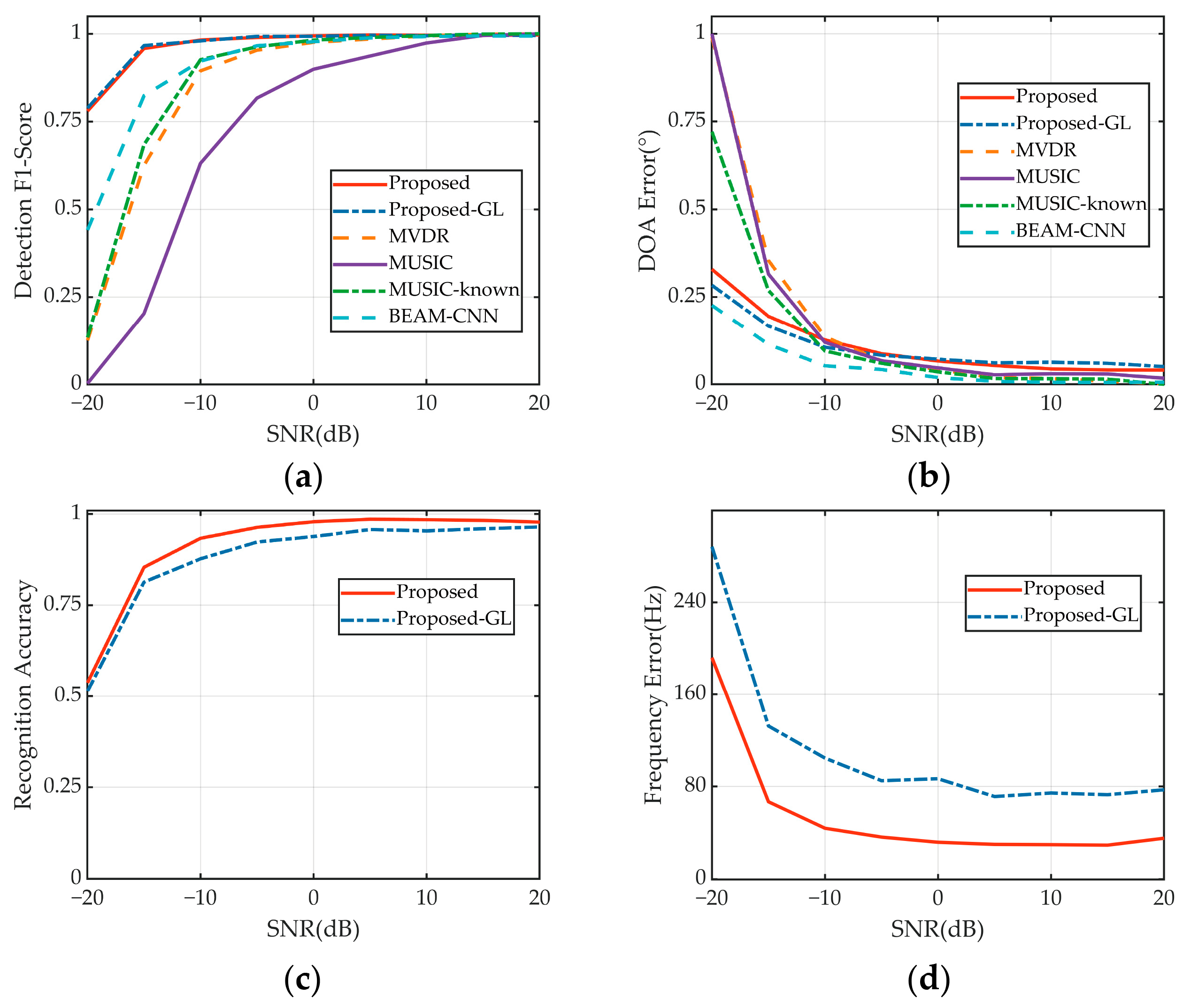
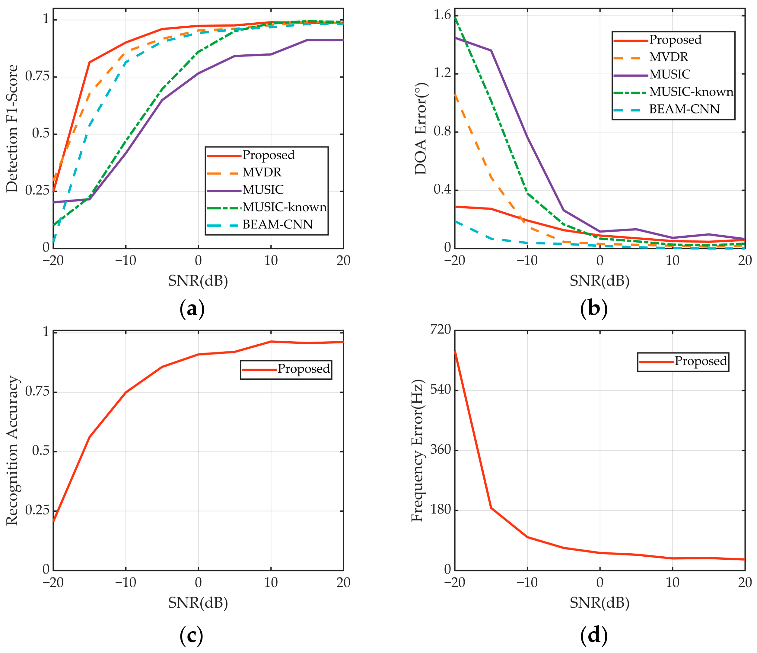
4.2. Performance at Different SNRs

All methods except proposed-GL were evaluated using test set I. Proposed-GL refers to the proposed method that was tested on test set II, because the carrier frequency range of 5–15 kHz exceeded the center frequency of the array (10 kHz), causing grating lobes. Test set II also featured a frequency distribution beyond the range of the training set, challenging the generalization capabilities of the model.

Despite the absence of grating lobe data during training, the proposed method maintained robust detection and DOA estimation performance on test set II, which included grating lobe data (Figure 5). However, their presence affected the signal modulation recognition and frequency band estimation performance of the model because grating lobes, while not altering the fundamental representation of the signal in the FRAZ spectrum, influence adjacent spectral features, thereby complicating model identification tasks and frequency band estimations. Notably, the proposed model achieved better DOA estimation results on test set II than on test set I. This can be attributed to the higher signal frequency, leading to a narrower and more concentrated main lobe on the DOA axes.

Figure 5. Prediction results obtained at various SNRs. (a) Detection performance. (b) DOA estimation. (c) Modulation recognition. (d) Frequency band estimation.

The proposed method demonstrates joint prediction performance at various SNRs that is superior to those of other methods (Figure 5). Specifically, while the detection performance of all methods deteriorates with decreasing SNR, that of the proposed method deteriorates less. Notably, at SNRs below 0 dB, the proposed method significantly outperforms other approaches. When the SNR is −15 dB, the proposed method maintains a detection F1 score of 0.96, significantly outperforming Beam-CNN (0.82), MUSIC-known (0.68), MVDR (0.62), and MUSIC (0.20). The detection performance of the MUSIC algorithm is adequate when the number of signal sources is unknown, but it markedly improves when this number is known. Under the simulation conditions, which include no statistical signal mismatch, MVDR performance is comparable to that of MUSIC with a known number of signal sources. BEAM-CNN performs slightly better at detection than the traditional algorithms. However, the proposed method excels under all SNR conditions because of its integrated use of spatial and frequency-domain signals. The DOA estimation errors for all methods tend to stabilize when the SNR exceeds −10 dB (Figure 5b). Below this threshold, deep-learning methods such as the proposed model estimate the DOA better.

As shown in Figure 5c,d, the proposed method accurately recognizes the signal modulation format, but its frequency band estimation error is notably influenced by the SNR. Specifically, when the SNR exceeds −10 dB, the modulation recognition and frequency band estimation results stabilize and are satisfactory. At −15 dB, the proposed method still achieves a recognition accuracy of 0.85 and a frequency band estimation error of 66.75 Hz, while Proposed-GL records accuracy and error rates of 0.81 and 132.48 Hz, respectively. In summary, the proposed method effectively performs the joint prediction task across various SNRs. It not only surpasses other methods in detection and DOA estimation but also reliably estimates the signal modulation format and frequency band.

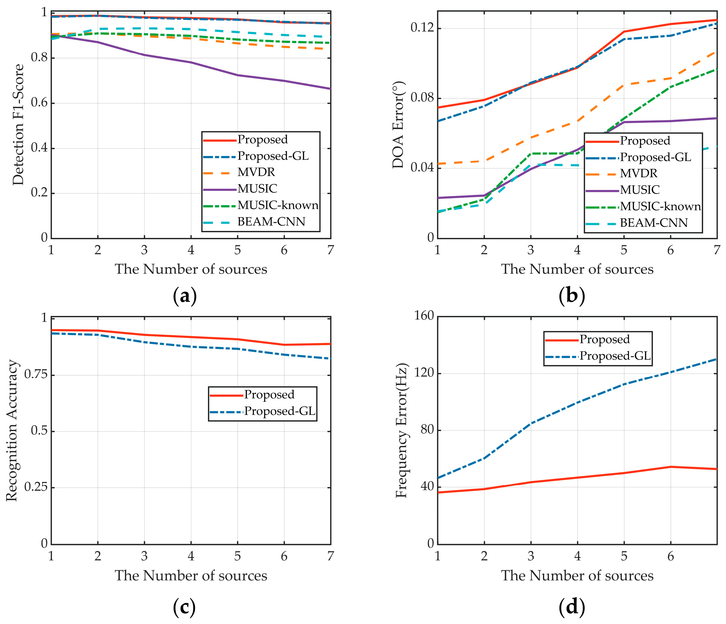
4.3. Performance Based on the Number of Sources

Proposed-GL was executed on test set II, whereas the remaining methods were evaluated on test set I. The detection performance of all methods degrades as the number of signals increases, a trend particularly pronounced for MUSIC (Figure 6a). However, the proposed method is the least sensitive to the number of signals. When handling seven UWAC signals, the proposed method achieves a detection F1 score of 0.95, substantially surpassing Beam-CNN at 0.89, MUSIC-known at 0.87, MVDR at 0.84, and MUSIC at 0.66. It effectively detects UWAC signals when the frequencies and DOA do not completely overlap while simultaneously estimating the number of UWAC sources. Hence, it is well suited for the joint prediction of multiple sources. Figure 6b reveals a uniform reduction in DOA estimation accuracy across all methods as the number of sources increases. Notably, the proposed method shows the weakest DOA estimation, which can be attributed to its relatively poor performance at high SNR levels.

Figure 6. Prediction results for different numbers of sources. (a) Detection performance. (b) DOA estimation. (c) Modulation recognition. (d) Frequency band estimation.

Both the recognition and frequency estimation performance of the proposed method moderately decline as the number of sources increases (Figure 6c,d). This deterioration is particularly severe under conditions with grating lobes, as revealed by the results of proposed-GL. The presence of multiple grating lobes, which occur when several signals exceed the center frequency of the array, significantly amplifies interference, compounding the challenges of signal estimation.

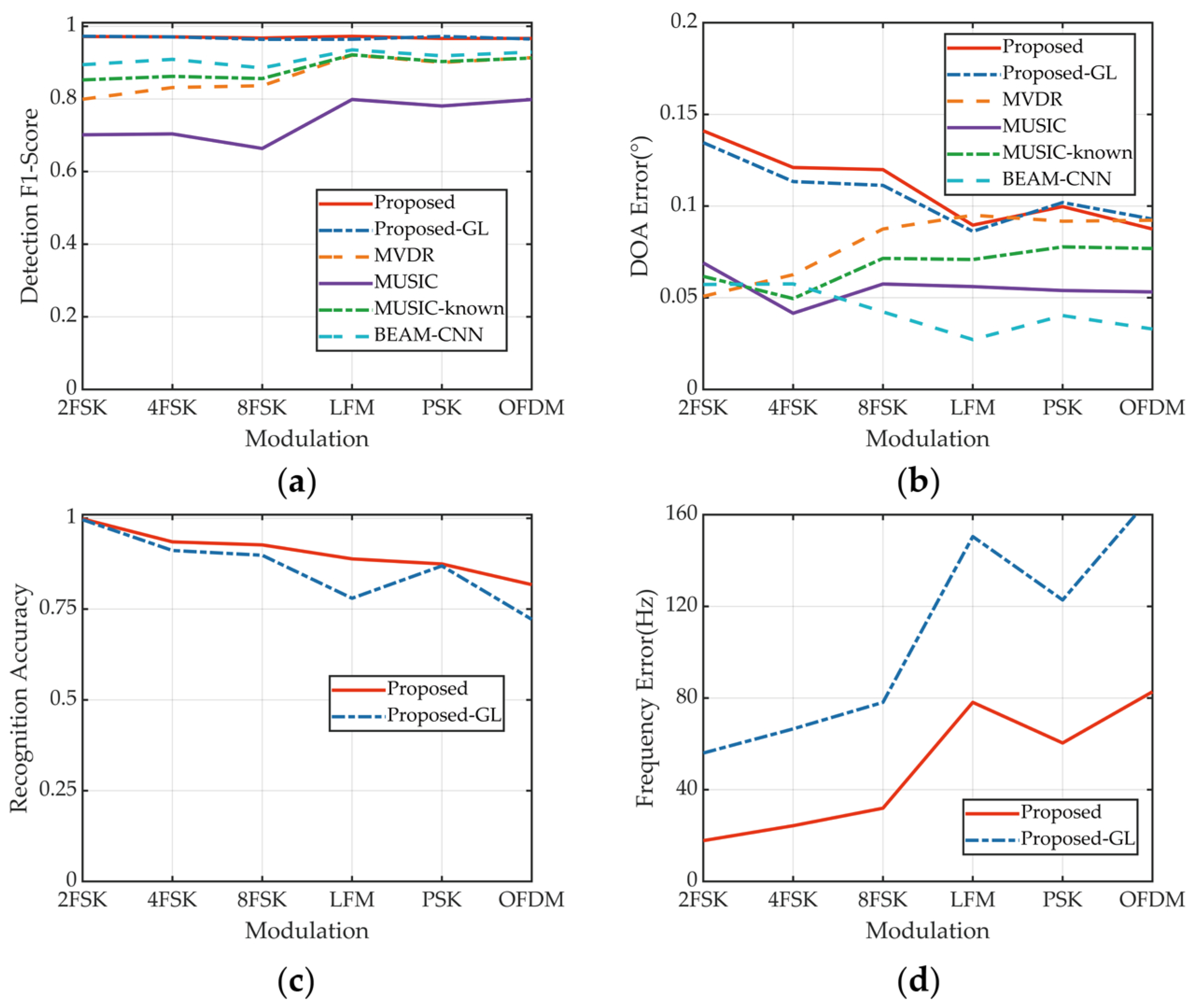
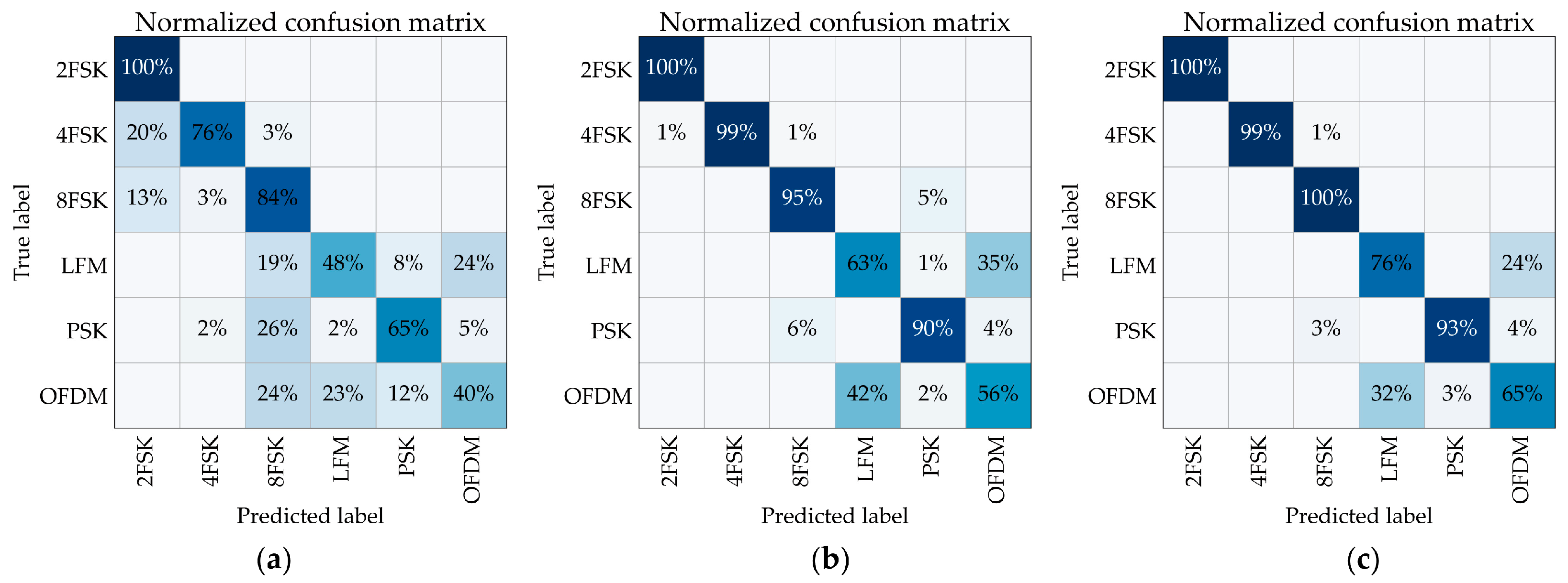
4.4. Performance for Different Modulations

Proposed-GL was evaluated on test set II, whereas other methods were assessed on test set I. The detection performance of the proposed method is consistent across various modulation formats (Figure 7a). In contrast, the other methods exhibit variable detection capabilities; they perform poorly on MFSK signals, which are discrete-frequency signals, but are more effective on broadband continuous signals such as PSK, LFM, and OFDM. The proposed method consistently achieves a detection F1 score of approximately 0.97 across all modulation methods. In contrast, the other methods perform best on LFM and worst on MFSK, with BEAM-CNN scoring 0.94 and 0.89, MUSIC-known scoring 0.92 and 0.85, and MVDR scoring 0.92 and 0.80, respectively. This variation can be attributed to the higher energy associated with broadband signals at the same in-band SNR. The traditional algorithms MVDR and MUSIC demonstrate superior DOA estimation for MFSK signals (Figure 7b). Conversely, the proposed method and BEAM-CNN achieve better DOA estimation for broadband continuous signals because of their pronounced characteristics.

Figure 7. Prediction results for different modulation types. (a) Detection performance. (b) DOA estimation. (c) Modulation recognition. (d) Frequency band estimation.

The proposed method excels in recognizing MFSK (Figure 7c), possibly because of its distinct spectral features. Broadband continuous signals, which tend to have less defined characteristics, pose more of a challenge for recognition. Similarly, the frequency-band estimation performance of the proposed method is more effective for MFSK because of the discrete and prominent point energy in its frequency spectrum.

4.5. Performance under Varying Signal Interference Levels

The resilience of the proposed method to various levels of signal interference was evaluated using test set III (see Figure 8). This test set uniquely included a constant strong interference signal at 30 dB, with other signals generated randomly within the parameter ranges. In contrast to other datasets, in which the maximum SNR difference among signals is capped at 20 dB, test set III challenges the i.i.d. assumption of learning-based methods.

Figure 8. Joint prediction results under different strength signal interference. (a) Detection performance. (b) DOA estimation. (c) Modulation recognition. (d) Frequency band estimation.

Therefore, the performance of all methods degraded under these conditions. In particular, MUSIC suffers significantly under strong signal interference, stabilizing only when the signal SNR exceeds 5 dB (Figure 8a). In contrast, because of its adaptive characteristics, the MVDR algorithm maintains robust detection capabilities even under intense interference, consistently outperforming BEAM-CNN at various SNR levels. Despite some performance losses, the proposed method still outperforms other techniques in detection accuracy. The proposed method demonstrates a more pronounced performance advantage under conditions of strong signal interference compared to scenarios with no interference. Specifically, at an SNR of −15 dB, it maintains a detection F1 score of 0.81, which significantly surpasses those of Beam-CNN at 0.54, MUSIC-known at 0.22, MVDR at 0.68, and MUSIC at 0.20.

While MVDR and MUSIC achieve precise DOA estimates at SNRs above 0 dB, their accuracy deteriorates sharply below this threshold (Figure 8b). Conversely, both the proposed method and BEAM-CNN maintain stable DOA estimation errors across a range of SNRs, proving resilient even under strong interference (below 0 dB).

Figure 8c,d present the effect of strong interference on the ability of the proposed method to recognize UWAC signal modulation formats and estimate frequency bands. Although performance degrades owing to the interference, the proposed method is considerably resilient, suggesting potential for further improvement if retrained with data that include interference signals.

4.6. Performance across Various Array Structure Parameters

Deep learning methods typically require retraining when applied to arrays with differing structural parameters to satisfy the i.i.d. assumption between training and test data. Nonetheless, the proposed method and BEAM-CNN are robust against variations in array structure. This resilience is attributed to the minimal effect of these parameters on the representation of local beams in the FRAZ spectrum.

Test set IV was used for all evaluations. This test set features signals collected by hydrophone arrays with 8 to 64 elements. By contrast, the training was exclusively conducted with data from 32-element hydrophone arrays. The detection performance of all methods improves as the number of array elements increases (Figure 9a). This improvement is particularly pronounced for MVDR and MUSIC, because the additional elements enhance the gain and resolution of the array. The proposed method and BEAM-CNN also benefit from these increases, as their inputs are derived from FRAZ spectrum and local beams. The generalization capabilities of the network and robustness of the input features enable these methods to adapt effectively to various arrays and maintain robust performance. For arrays with more than 24 elements, the DOA estimation errors of the methods remain stable (Figure 9b). However, for MUSIC, the DOA estimation error decreases sharply when the array has fewer than 24 elements, while the errors for the other methods change marginally.

Figure 9. Prediction results of various number of hydrophone elements. (a) Detection performance. (b) DOA estimation. (c) Modulation recognition. (d) Frequency band estimation.

The accuracy of signal modulation format recognition improves as the number of array elements increases (Figure 9c). Notably, the modulation format recognition rate exhibits no loss when the number of elements exceeds 32, demonstrating the effectiveness of the model even without training data encompassing such configurations. The bandwidth-estimation ability of the proposed method deteriorates only when the number of array elements decreases (Figure 9d). This demonstrates the strong generalization capabilities of our method across a range of array structures.

5. Experimental Studies

To further evaluate the generalizability and joint prediction capabilities of the proposed method in real-world environments, we conducted extensive experiments using actual experimental data. Initially, simulated UWAC signals were generated using the BELLHOP [51] acoustic simulation model, incorporating both simulated acoustic signals and actual experimental environment noise. We then assessed the practicality and generalization ability of the proposed method by comparing its performance across three training scenarios combining simulated data and experimental data.

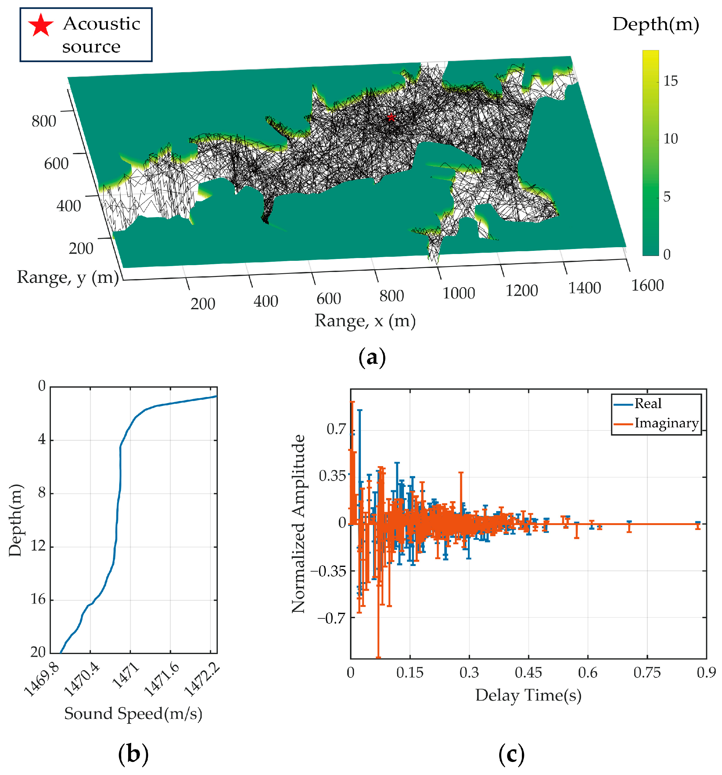
5.1. UWAC Signal Simulation and Experiment

The BELLHOP model, which is based on ray tracing, simulates sound wave propagation and interactions within complex underwater environments, particularly for UWAC scenarios involving multipath propagation. We used BELLHOP to emulate the UWAC channel. To replicate real-world conditions, we incorporated the actual terrain of the lake under examination, which introduced pronounced reverberation effects, surpassing those observed in free space. Additionally, we used measured sound speed profiles (SSPs) specific to the lake environment. These SSPs (Figure 10b) reflected the unique acoustic characteristics of the lake. Figure 10a presents a comprehensive acoustic ray-tracing example, in which sound rays interact with the lake boundary, resulting in multiple reflections and substantial reverberation effects. Consequently, the received UWAC signal is substantially distorted. Figure 10c presents the simulated channel impulse response, revealing over 500 multipaths, with the longest multipath length lasting approximately 0.9 s.

Figure 10. (a) Acoustic ray tracing in lake terrain. (b) Sound speed profile on the lake. (c) Simulated channel impulse response based on BELLHOP.

Using the impulse response derived from the simulation, the UWAC signal passing through the multipath channel was modeled using convolutions to introduce frequency-selective fading into the received signal. Additionally, to model the relative motion typically present between the signal source and receiver, a Doppler shift was incorporated, resulting in time-selective fading. Severe multipath effects are evident in the spectrograms of the simulated and experimental PSK signals, with significant multipath delay spread observable in Figure 11a,b. The FRAZ spectra in Figure 11c,d show some discrepancies between the simulated and experimental signals because of unmodeled small-scale fading. For a more detailed discussion on the accurate modeling of the UWAC channel, see [52].

Figure 11. Spectrograms and FRAZ spectra of signals with normalized intensity, indicated by brighter colors representing higher energy levels. (a) Spectrograms of the simulated PSK signal. (b) Spectrograms of the experimental PSK signal. (c) FRAZ spectrum of the simulated PSK signal. (d) FRAZ spectrum of the experimental PSK signal.

In this experiment, a thin fiber-optic hydrophone array was used for the UWAC signal reception, as detailed in [53]. We selected 23 hydrophone elements, and the array element spacing was 0.075 m with a center frequency of 10,000 Hz. The details of the FRAZ spectrum generation and model training were the same as those of the simulation; however, the emission signals were different. During the lake tests, an acoustic transducer with a frequency range of 7000–14,000 Hz was used. The frequency of the test signal was within this range, which caused grating lobes. Six modulation formats were used to modulate the signal (2FSK, 4FSK, 8FSK, BPSK, LFM, and OFDM), which had an SNR of approximately 20 dB. However, in each experiment, only one signal in one format was transmitted and detected at a time. The parameters generated by the simulated signal were consistent with the actual data parameters.

During the experiment, we positioned the fiber-optic hydrophone array in the lake and hung it at a depth of 5 m. The UWAC signal was then emitted from a sound source towed by a vessel at a speed of approximately four knots, following the GPS trajectory in the recording shown in Figure 12. The GPS tracks and bearing time records (BTRs) of the training data are shown in Figure 12a and Figure 12b, respectively. The training and test data were collected on separate days. During the experiment, a 4 s pause was introduced after each signal was emitted.

Figure 12. (a) GPS track and (b) GPS BTR of the training data. (c) GPS track and (d) GPS BTR of the test data.

The training and testing configurations were aligned with the protocols established in the simulation experiments. In this analysis, we developed three distinct models: “simulation trained”, which was trained exclusively on 12,000 simulated signals; “experiment trained”, which used 1481 signals collected from experimental data; and “mixed trained”, which combined 3000 simulated signals with 1481 experimentally collected signals. These models were then assessed using a test set that comprised 1582 experimentally acquired signals. Additionally, we performed evaluations using continuous-time signals for each model to estimate the BTRs.

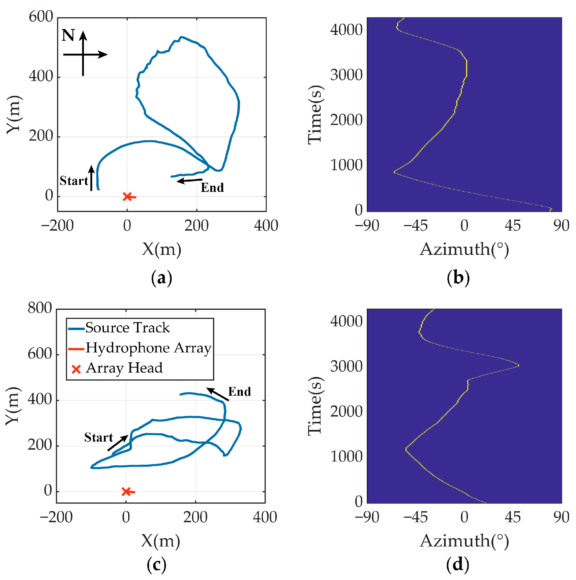
5.2. Experimental Results

Among the models trained on the three datasets across various modulations, each model demonstrated robust joint prediction capabilities. Notably, the simulation-trained model performed well. This result underscores the superior generalization ability and practical utility of the proposed method, suggesting its potential for real-world applications, even in the absence of actual signal data.

The experiment-trained model demonstrates robust detection performance across all modulation formats (Figure 13a). However, the detection performance of the simulation-trained model is marginally lower for PSK-modulated signals. This discrepancy is likely attributed to the significant frequency-selective fading undergone by actual PSK signals and the substantial differences between the simulated and experimental signals. Despite these challenges, achieving a detection F1 score of 0.9 with only simulated signals underscores the strong potential of the proposed method for broad applicability in various scenarios, particularly those requiring accurate DOA estimation and joint prediction capabilities.

Figure 13. Joint prediction results from models trained on various datasets across different modulation formats. (a) Detection performance. (b) DOA estimation. (c) Modulation recognition. (d) Frequency band estimation.

All three models deliver commendable DOA estimation results (Figure 13b). Nonetheless, the simulation-trained model exhibits poorer DOA estimation performance for broadband continuous signals. This shortfall is primarily due to the significant discrepancies between the simulated and experimental signals. Incorporating real data into the training process markedly improves DOA estimation accuracy. Overall, the average detection F1 score and DOA error for the model trained solely on simulation data is 0.88 and 0.306°, while the model trained on experimental data achieves an average F1 score of 0.97 and DOA error 0.156°. The model trained on a mixed dataset of simulation and experimental data exhibits an even higher average F1 score of 0.985 and DOA error 0.156°.

The recognition accuracy for broadband signals decreases across all models in actual scenarios, primarily owing to the complex channel environment (Figure 13c). The channel effects reduce distinguishability among broadband signals. The simulation-trained model exhibits considerable confusion in identifying actual signals (Figure 14a), highlighting the substantial differences between the simulated and real channel characteristics for spectrum identification features. While the experiment-trained models yield minimal confusion among MFSK signals, significant confusion persists between the LFM and OFDM signals (Figure 14b). The mixed-training strategy employing both simulated and experimental data improves the recognition accuracy for all modulation types (Figure 14c). Thus, this hybrid training regimen enables the model to extract features that are more robust, thus enhancing the overall recognition accuracy.

Figure 14. Modulation recognition confusion matrix of the (a) simulation-trained, (b) experiment-trained, and (c) mixed-trained models.

The frequency band of MFSK signals can be accurately estimated using only simulated training data (Figure 13d). However, the estimation performance for broadband continuous signals is less robust, largely owing to discrepancies between the simulated and actual channel characteristics. This challenge can be mitigated by incorporating experimental data into the training process. Notably, employing simulation data to augment the experimental data significantly enhances the joint prediction capabilities of the proposed method. This approach of data expansion is not only beneficial in this context but can also be applied to other signal parameter estimation applications.

To assess the continuous DOA estimation capabilities of the proposed model, we analyzed the data measured between 2590 and 3590 s from the test dataset. The GPS BTRs of the towing ship obtained during the experiment are shown in Figure 15a. During the experiment, while the UWAC signals were being transmitted, an electric boat was observed in the distance, moving between −80° to 0° relative to the array. The DOA tracking trajectory of the boat is distinctly delineated in the MUSIC BTRs. Owing to the inadequate signal energy and uncertainty in the frequency bandwidth, the UWAC signals within the BTRs generated using CBF lack sufficient clarity. In contrast, the UWAC signal targets estimated by MUSIC and MVDR are more obvious.

Figure 15. Normalized bearing time recordings depicted with brighter colors to represent higher energy levels of (a) GPS, (b) CBF, (c) MVDR, (d) MUSIC, (e) BEAM-CNN, (f) simulation-trained, (g) experiment-trained, and (h) mixed-trained models.

BEAM-CNN, which was trained using experimental data, struggled to detect many UWAC signals, particularly those with azimuthal angles exceeding 30°. This may be attributed to the scarcity of training samples featuring DOAs over 30° (Figure 12b), limiting the detection capabilities of BEAM-CNN in this range. The proposed model, even when trained solely on simulation data, successfully detects most signals with trajectories that are clearly visible (Figure 15g). Notably, the proposed model can not only delineate clear beam trajectories for UWAC signals but also detect the distant electric boat. This may have occurred because the model occasionally confused the spectral characteristics of the ship with those of communication signals. When trained with experimental data, the model enhanced its feature learning for UWAC signals, reducing such confusion. Using mixed or just experimental data for training substantially increases detection confidence (Figure 15g,h).

Overall, both simulation and experimental studies have demonstrated the effectiveness of the proposed method. In simulations, it consistently outperforms traditional methods in detection and joint prediction tasks, while achieving DOA estimation performance comparable to that of traditional methods. Notably, the proposed method exhibits superior detection performance across all SNRs, with particularly significant advantages at lower SNRs. Additionally, as the number of signal sources increases, the proposed method experiences minimal loss in detection performance. Its effectiveness remains consistent regardless of the modulation type of the UWAC signal, contrasting with traditional methods that show diminished performance in MFSK modulation. When faced with strong signal interference, the proposed method maintains excellent detection performance by fully utilizing the frequency band information of the signal. Unlike deep learning frameworks that depend on the input of spatial covariance matrices or raw signals, our method can adapt to arrays with varying numbers of elements without retraining, and its joint prediction performance improves as the number of elements increases.

In experimental studies, the proposed method demonstrates strong viability and generalizability in practical scenarios. It achieves excellent joint prediction of actual UWAC signals, even when relying solely on simulation data or a limited subset of experimental data. This indicates that in new UWAC environments, effective detection of signals can be accomplished by merely collecting ambient noise and synthesizing it through simulation.

6. Conclusions

We introduced a joint prediction method for multiple UWAC signals detection. Based on the FRAZ spectrum and Faster R-CNN framework, our method effectively performs joint prediction tasks, including signal detection, modulation recognition, frequency band and DOA estimation. Simulation and experimental studies have been conducted across various scenarios to demonstrate the effectiveness of the proposed method in joint prediction. The proposed method consistently outperforms traditional methods in detection performance. Its joint prediction capability remains robust across various signal modulation types and is resilient to strong signal interference. It can estimate and detect multiple wideband UWAC signals and excels in the presence of grating lobes. Compared to other deep learning-based methods, our method requires less training data and remains effective without the need for retraining when the number of array elements changes. The proposed method can also efficiently perform joint prediction in real-world scenarios and maintain robustness, even when trained on solely simulated data or limited experimental data.

These results demonstrate the potential of our method in various array-based systems requiring joint predictions, including other sonar systems, wireless antenna arrays, and microphones. However, recognizing continuous broadband signals in experiments remains a challenge. Future research will aim to address this limitation by refining our approach to enhance its applicability and performance.

References

- Singer, A.C.; Nelson, J.K.; Kozat, S.S. Signal processing for underwater acoustic communications. IEEE Commun. Mag. 2009, 47, 90–96. [Google Scholar] [CrossRef]
- Lu, H.; Jiang, M.; Cheng, J. Deep learning aided robust joint channel classification, channel estimation, and signal detection for underwater optical communication. IEEE Trans. Commun. 2021, 69, 2290–2303. [Google Scholar] [CrossRef]
- Luo, X.; Shen, Z. A space-frequency joint detection and tracking method for line-spectrum components of underwater acoustic signals. Appl. Acoust. 2021, 172, 107609. [Google Scholar] [CrossRef]
- Ren, S.; He, K.; Girshick, R.; Sun, J. Faster R-CNN: Towards real-time object detection with region proposal networks. In Proceedings of the Advances in Neural Information Processing Systems 28 (NIPS 2015), Montreal, QC, Canada, 7–12 December 2015; Volume 28, pp. 91–99. [Google Scholar]
- Han, K.; Nehorai, A. Improved source number detection and direction estimation with nested arrays and ULAs using jackknifing. IEEE Trans. Signal Process. 2013, 61, 6118–6128. [Google Scholar] [CrossRef]
- Johnson, D.H.; Dudgeon, D.E. Array Signal Processing: Concepts and Techniques; Prentice-Hall: Englewood Cliffs, NJ, USA, 1992. [Google Scholar]
- Schmidt, R.O. Multiple emitter location and signal parameter estimation. IEEE Trans. Antennas Propag. 1986, 34, 276–280. [Google Scholar] [CrossRef]
- Roy, R.; Kailath, T. ESPRIT-estimation of signal parameters via rotational invariance techniques. IEEE Trans. Acoust. Speech Signal Process. 1989, 37, 984–995. [Google Scholar] [CrossRef]
- Rao, B.; Hari, K. Performance analysis of root-Music. IEEE Trans. Acoust. Speech Signal Process. 1989, 37, 1939–1949. [Google Scholar] [CrossRef]
- Capon, J. High-resolution frequency-wavenumber spectrum analysis. Proc. IEEE 1969, 57, 1408–1418. [Google Scholar] [CrossRef]
- Frost, O. An algorithm for linearly constrained adaptive array processing. Proc. IEEE 1972, 60, 926–935. [Google Scholar] [CrossRef]
- Zhang, L.; Liu, W.; Langley, R.J. A class of constrained adaptive beamforming algorithms based on uniform linear arrays. IEEE Trans. Signal Process. 2010, 58, 3916–3922. [Google Scholar] [CrossRef]
- Liu, Y.; Chen, H.; Wang, B. DOA estimation based on CNN for underwater acoustic array. Appl. Acoust. 2021, 172, 107594. [Google Scholar] [CrossRef]
- Ozanich, E.; Gerstoft, P.; Niu, H. A feedforward neural network for direction-of-arrival estimation. J. Acoust. Soc. Am. 2020, 147, 2035–2048. [Google Scholar] [CrossRef] [PubMed]
- Feintuch, S.; Tabrikian, J.; Bilik, I.; Permuter, H. Neural-network-based DOA estimation in the presence of non-Gaussian interference. IEEE Trans. Aerosp. Electron. Syst. 2024, 60, 119–132. [Google Scholar] [CrossRef]
- Zhang, Y.; Huang, Y.; Tao, J.; Tang, S.; So, H.C.; Hong, W. A Two-stage multi-layer perceptron for high-resolution doa estimation. IEEE Trans. Veh. Technol. 2024, 1–16. [Google Scholar] [CrossRef]
- Guo, Y.; Zhang, Z.; Huang, Y. Dual class token vision transformer for direction of arrival estimation in low SNR. IEEE Signal Process. Lett. 2024, 31, 76–80. [Google Scholar] [CrossRef]
- Chakrabarty, S.; Habets, E.A.P. Multi-speaker DOA estimation using deep convolutional networks trained with noise signals. IEEE J. Sel. Top. Signal Process. 2019, 13, 8–21. [Google Scholar] [CrossRef]
- Papageorgiou, G.K.; Sellathurai, M.; Eldar, Y.C. Deep networks for direction-of-arrival estimation in low SNR. IEEE Trans. Signal Process. 2021, 69, 3714–3729. [Google Scholar] [CrossRef]
- Nie, W.; Zhang, X.; Xu, J.; Guo, L.; Yan, Y. Adaptive direction-of-arrival estimation using deep neural network in marine acoustic environment. IEEE Sens. J. 2023, 23, 15093–15105. [Google Scholar] [CrossRef]
- Zheng, S.; Yang, Z.; Shen, W.; Zhang, L.; Zhu, J.; Zhao, Z.; Yang, X. Deep learning-based DOA estimation. IEEE Trans. Cogn. Commun. Netw. 2024, 10, 819–835. [Google Scholar] [CrossRef]
- Cong, J.; Wang, X.; Huang, M.; Wan, L. Robust DOA estimation method for MIMO radar via deep neural networks. IEEE Sens. J. 2021, 21, 7498–7507. [Google Scholar] [CrossRef]
- Merkofer, J.P.; Revach, G.; Shlezinger, N.; Routtenberg, T.; van Sloun, R.J.G. DA-MUSIC: Data-driven DoA estimation via deep augmented MUSIC algorithm. IEEE Trans. Veh. Technol. 2024, 73, 2771–2785. [Google Scholar] [CrossRef]
- Wu, L.-L.; Liu, Z.-M.; Huang, Z.-T. Deep convolution network for direction of arrival estimation with sparse prior. IEEE Signal Process. Lett. 2019, 26, 1688–1692. [Google Scholar] [CrossRef]
- Bell, C.J.; Adhikari, K.; Freeman, L.A. Convolutional neural network-based regression for direction of arrival estimation. In Proceedings of the 2023 IEEE 14th Annual Ubiquitous Computing, Electronics & Mobile Communication Conference (UEMCON), New York, NY, USA, 12–14 October 2023; pp. 373–379. [Google Scholar]
- Cai, R.; Tian, Q. Two-stage deep convolutional neural networks for DOA estimation in impulsive noise. IEEE Trans. Antennas Propag. 2024, 72, 2047–2051. [Google Scholar] [CrossRef]
- Prasad, K.N.R.S.V.; D’Souza, K.B.; Bhargava, V.K. A Downscaled faster-RCNN framework for signal detection and time-frequency localization in wideband RF systems. IEEE Trans. Wirel. Commun. 2020, 19, 4847–4862. [Google Scholar] [CrossRef]
- O’Shea, T.; Roy, T.; Clancy, T.C. Learning robust general radio signal detection using computer vision methods. In Proceedings of the 2017 51st Asilomar Conference on Signals, Systems, and Computers, Pacific Grove, CA, USA, 29 October–1 November 2017; pp. 829–832. [Google Scholar]
- Nguyen, H.N.; Vomvas, M.; Vo-Huu, T.D.; Noubir, G. WRIST: Wideband, real-time, spectro-temporal RF identification system using deep learning. IEEE Trans. Mob. Comput. 2023, 23, 1550–1567. [Google Scholar] [CrossRef]
- Cheng, L.; Zhu, H.; Hu, Z.; Luo, B. A Sequence-to-Sequence Model for Online Signal Detection and Format Recognition. IEEE Signal Process. Lett. 2024, 31, 994–998. [Google Scholar] [CrossRef]
- Adavanne, S.; Politis, A.; Nikunen, J.; Virtanen, T. Sound event localization and detection of overlapping sources using convolutional recurrent neural networks. IEEE J. Sel. Top. Signal Process. 2019, 13, 34–48. [Google Scholar] [CrossRef]
- He, W.; Motlicek, P.; Odobez, J.-M. Adaptation of multiple sound source localization neural networks with weak supervision and domain-adversarial training. In Proceedings of the ICASSP 2019—2019 IEEE International Conference on Acoustics, Speech and Signal Processing (ICASSP), Brighton, Great Britain, 12–17 May 2019; pp. 770–774. [Google Scholar]
- Le Moing, G.; Vinayavekhin, P.; Agravante, D.J.; Inoue, T.; Vongkulbhisal, J.; Munawar, A.; Tachibana, R. Data-efficient framework for real-world multiple sound source 2D localization. In Proceedings of the ICASSP 2021—2021 IEEE International Conference on Acoustics, Speech and Signal Processing (ICASSP), Toronto, ON, Canada, 6–11 June 2021; pp. 3425–3429. [Google Scholar]
- Schymura, C.; Bönninghoff, B.; Ochiai, T.; Delcroix, M.; Kinoshita, K.; Nakatani, T.; Araki, S.; Kolossa, D. PILOT: Introducing transformers for probabilistic sound event localization. In Proceedings of the Interspeech 2021, Brno, Czech Republic, 30 August–3 September 2021. [Google Scholar]
- Ranjan, R.; Jayabalan, S.; Nguyen, T.N.T.; Gan, W.S. Sound event detection and direction of arrival estimation using residual net and recurrent neural networks. In Proceedings of the 4th Workshop on Detection and Classification of Acoustic Scenes and Events (DCASE 2019), New York, NY, USA, 25–26 October 2019. [Google Scholar]
- Yasuda, M.; Koizumi, Y.; Saito, S.; Uematsu, H.; Imoto, K. Sound event localization based on sound intensity vector refined by DNN-based denoising and source separation. In Proceedings of the ICASSP 2020–2020 IEEE International Conference on Acoustics, Speech and Signal Processing (ICASSP), Barcelona, Spain, 4–8 May 2020; pp. 651–655. [Google Scholar]
- Chytas, S.; Potamianos, G. Hierarchical detection of sound events and their localization using convolutional neural networks with adaptive thresholds. In Proceedings of the Detection and Classification of Acoustic Scenes and Events 2019 Workshop (DCASE2019), New York, NY, USA, 25–26 October 2019; pp. 50–54. [Google Scholar]
- Sundar, H.; Wang, W.; Sun, M.; Wang, C. Raw waveform based end-to-end deep convolutional network for spatial localization of multiple acoustic sources. In Proceedings of the 2020 IEEE International Conference on Acoustics, Speech and Signal Processing (ICASSP), Barcelona, Spain, 4–8 May 2020; pp. 4642–4646. [Google Scholar]
- He, Y.; Trigoni, N.; Markham, A. SoundDet: Polyphonic moving sound event detection and localization from raw waveform. In Proceedings of the 38th International Conference on Machine Learning (ICML), Virtual, 18–24 July 2021. [Google Scholar]
- Chakrabarty, S.; Habets, E.A.P. Broadband DOA estimation using convolutional neural networks trained with noise signals. In Proceedings of the IEEE Workshop on Applications of Signal Processing to Audio and Acoustics (WASPAA), New Paltz, NY, USA, 15–18 October 2017; pp. 136–140. [Google Scholar]
- Diaz-Guerra, D.; Miguel, A.; Beltran, J.R. Robust sound source tracking using SRP-PHAT and 3D convolutional neural networks. IEEE/ACM Trans. Audio Speech Lang. Process. 2021, 29, 300–311. [Google Scholar] [CrossRef]
- Lu, Z. Sound event detection and localization based on CNN and LSTM. In Proceedings of the Detection and Classification of Acoustic Scenes and Events 2019 Workshop (DCASE2019), New York, NY, USA, 25–26 October 2019. [Google Scholar]
- Comanducci, L.; Borra, F.; Bestagini, P.; Antonacci, F.; Tubaro, S.; Sarti, A. Source localization using distributed microphones in reverberant environments based on deep learning and ray space transform. IEEE/ACM Trans. Audio Speech Lang. Process. 2020, 28, 2238–2251. [Google Scholar] [CrossRef]
- Vera-Diaz, J.M.; Pizarro, D.; Macias-Guarasa, J. Towards domain independence in CNN-based acoustic localization using deep cross correlations. In Proceedings of the 2020 28th European Signal Processing Conference (EUSIPCO), Amsterdam, The Netherlands, 18–21 January 2021; pp. 226–230. [Google Scholar]
- Gelderblom, F.B.; Liu, Y.; Kvam, J.; Myrvoll, T.A. Synthetic data for DNN-based DOA estimation of indoor speech. In Proceedings of the ICASSP 2021—2021 IEEE International Conference on Acoustics, Speech and Signal Processing (ICASSP), Toronto, ON, Canada, 6–11 June 2021; pp. 4390–4394. [Google Scholar]
- Neubeck, A.; Van Gool, L. Efficient non-maximum suppression. In Proceeding of the 18th International Conference on Pattern Recognition (ICPR’06), Hong Kong, China, 20–24 August 2006; pp. 850–855. [Google Scholar]
- He, K.; Gkioxari, G.; Dollár, P.; Girshick, R. Mask R-CNN. In Proceedings of the 2017 IEEE International Conference on Computer Vision (ICCV 2017), Venice, Italy, 22–29 October 2017; pp. 2961–2969. [Google Scholar]
- Jaderberg, M.; Simonyan, K.; Zisserman, A. Spatial transformer networks. In Proceedings of the Annual Conference on Neural Information Processing Systems 2015, Montreal, QC, Canada, 7–12 December 2015; pp. 2017–2025. [Google Scholar]
- Wax, M.; Kailath, T. Detection of signals by information theoretic criteria. IEEE Trans. Acoust. Speech Signal Process. 1985, 33, 387–392. [Google Scholar] [CrossRef]
- He, K.; Zhang, X.; Ren, S.; Sun, J. Deep residual learning for image recognition. In Proceedings of the IEEE Computer Society Conference on Computer Vision and Pattern Recognition (CVPR), Las Vegas, NV, USA, 27–30 June 2016; pp. 770–778. [Google Scholar]
- Porter, M.B. The BELLHOP Manual and User’s Guide: Preliminary Draft; Heat Light Sound Research Inc.: La Jolla, CA, USA, 2011; Available online: http://oalib.hlsresearch.com/Rays/HLS-2010-1.pdf (accessed on 16 January 2024).
- Qarabaqi, P.; Stojanovic, M. Statistical characterization and computationally efficient modeling of a class of underwater acoustic communication channels. IEEE J. Ocean. Eng. 2013, 38, 701–717. [Google Scholar] [CrossRef]
- Liu, Y.; Cheng, L.; Zou, Y.; Hu, Z. Thin Fiber-Optic Hydrophone Towed Array for Autonomous Underwater Vehicle. IEEE Sens. J. 2024, 24, 15125–15132. [Google Scholar] [CrossRef]
Disclaimer/Publisher’s Note: The statements, opinions and data contained in all publications are solely those of the individual author(s) and contributor(s) and not of MDPI and/or the editor(s). MDPI and/or the editor(s) disclaim responsibility for any injury to people or property resulting from any ideas, methods, instructions or products referred to in the content. |
© 2024 by the authors. Licensee MDPI, Basel, Switzerland. This article is an open access article distributed under the terms and conditions of the Creative Commons Attribution (CC BY) license (https://creativecommons.org/licenses/by/4.0/).