1. Introduction
As the battlefield environment becomes increasingly complex, radar jamming has become more prevalent. Radar jamming is a serious threat to radar systems in electronic warfare, disrupting target detection, identification, and tracking [
1,
2]. Therefore, to acquire a real target and its parameters, anti-jamming techniques are widely used to improve the performance of radar systems. As a fundamental prerequisite, the effective recognition of radar jamming types provides significant support for implementing appropriate anti-jamming techniques. Namely, accurate radar jamming recognition plays a critical role in ensuring the survival and effectiveness of radar systems on the battlefield [
3,
4].
The existing methods for the radar jamming recognition task mainly focus on supervised learning, which depends on strong supervision information (i.e., adequate training samples with high-quality labels). However, the collected samples in real applications often come with weak supervision information (i.e., noisy or unlabeled training samples), making it challenging to achieve good recognition performance. Weakly supervised learning has shown effectiveness under weak supervision in the areas of natural language processing [
5], computer vision [
6], and imaging radar applications [
7]. Yet, there are no specific weakly supervised learning methods for the radar jamming recognition task. Next, a comprehensive overview of the existing research will be described in detail.
Supervised learning-based methods for radar jamming recognition: In recent decades, many supervised learning methods have been proven to be effective for radar jamming recognition tasks. These methods can mainly be divided into two categories: traditional feature extraction-based methods and deep learning-based methods. The overview of traditional feature extraction-based methods can be described as follows: First, distinguishing features are extracted from the time domain [
8], frequency domain [
9], time-frequency [
10] domain, and transform domain [
11]. Then, these features are provided to a machine learning model for training [
12,
13]. However, traditional feature extraction-based methods usually rely on the hand-crafted feature extraction acquired by experts, which poses a disadvantage in ensuring excellent recognition performance.
To overcome the shortcomings of traditional feature extraction-based methods, deep convolutional neural network (CNN)-based methods [
14] were introduced in the field of radar jamming recognition. These methods have the advantage of extracting powerful features. Specifically, in contrast to traditional feature extraction-based methods, CNN-based methods work through a layer-by-layer feature transformation process, where the features of the original data are progressively transformed into a new feature space, that is, CNN-based methods can further extract more discriminative features automatically and thus usually achieve superior recognition performance [
15]. According to the format of the input radar jamming signal, these CNN-based methods can be divided into one-dimensional methods [
16,
17] and two-dimensional methods [
18,
19]. For one-dimensional methods, radar jamming echo sequences are directly fed into deep-learning models [
20,
21]. Unlike one-dimensional methods, for two-dimensional methods, echo sequences are usually transformed into radar jamming images using a short-time Fourier transform. Then, these images are used as inputs for models [
22,
23].
Transformer-based methods for radar jamming recognition: CNN-based methods extract features by sliding convolutional kernels over the radar jamming signal, and each convolutional kernel can only extract local features within its receptive field [
24]. Therefore, the aforementioned one-dimensional and two-dimensional CNN-based methods have restrictions on learning long-range relationships between sampling points of radar jamming. Recently, the Transformer (TR) [
25] has been widely reported due to its global dependency extraction capability, which has achieved attractive achievements in many fields [
26]. The self-attention mechanism effectively allows the TR to capture dependencies across arbitrary sampling points. Thus, the TR enables the extraction of global features of the radar jamming signal without being limited by the distance between sampling points. The advantages of the TR prompt researchers to explore more suitable frameworks to improve radar jamming recognition accuracy. Analogously, based on the format of the input radar jamming signal, TR-based methods can also be divided into one-dimensional-based methods [
27] and two-dimensional-based methods [
28], which achieve higher accuracy compared to CNN-based methods owing to the remarkable capability of modeling long-distance relationships in the TR. Thus, using the TR is a more suitable method for long radar jamming sequences.
In summary, the aforementioned deep learning-based methods (i.e., CNN-based methods and TR-based methods) all belong to supervised learning methods, which depend on high-quality labels and enough labeled training samples. Although these supervised learning methods have shown superior performance in radar jamming recognition tasks, the collected radar jamming samples in practice often lack good supervision information, leading to a drop in recognition performance. Specifically, on the one hand, the accurate labeling of samples is challenging due to human and nonhuman factors. On the other hand, it is extremely difficult to obtain sufficient labeled training samples on the complex battlefield because of the limitations of security, technology, and so on. Accordingly, the obtained radar jamming samples may contain noisy samples (i.e., mislabeled samples) and plenty of unlabeled samples. Both noisy samples and unlabeled samples lead to a negative impact on recognition accuracy. That is to say, noisy samples or the lack of sufficient labeled training samples make it more challenging to accurately recognize radar jamming types. Therefore, it is highly desirable to address this problem using specialized methods. The great success of machine learning has promoted the development of radar signal processing.
Weakly supervised learning: Weakly supervised learning is an umbrella term that lightens the requirements of strong labels by learning with mislabeled or unlabeled data, and it consists of three typical types: incomplete supervision, inexact supervision, and inaccurate supervision [
29]. To this end, weakly supervised learning provides a direction to alleviate the problem of a reduction in recognition performance under radar jamming samples with weak labels. According to the definition of weak supervision in [
29], the radar jamming recognition task in the presence of noisy samples and unlabeled samples belongs to inaccurate supervision and incomplete supervision, respectively.
For inaccurate supervision, mislabels, namely unreliable labels, are called noisy labels, where annotated labels are different from ground-truth labels [
30]. As research on inaccurate supervision has deepened, noisy labels have been widely discussed [
31]. In detail, due to manual labeling errors (a lack of professionalism), raw data noise, and other issues, data with noisy labels are inevitable [
32]. Simultaneously, when there are noisy labels in the dataset, the model tends to overfit these noisy labels, making it less generalizable. To ensure recognition performance is improved, first, the samples with noisy labels should be judged. Then, the harmful effects on recognition performance caused by noisy samples should be reduced during the training process.
For incomplete supervision, there are only a few labeled samples, and the rest are un-labeled samples [
33]. The issue of the degradation of recognition performance caused by inadequate labeled training samples should be noticed. Semi-supervised learning (SSL) is a powerful tool for solving this problem. It uses the model itself to assign pseudo labels (PL) to unlabeled samples. Following this, high-confidence (above the defined confidence threshold) pseudo-labeling samples are treated as labeled samples. These samples are then added to the training set. Therefore, instead of using labeled samples alone, both labeled and unlabeled samples are simultaneously utilized in SSL to train a recognizer. As a result, underlying data properties are better captured in SSL, which leads to an improvement in recognition performance with plenty of unlabeled samples. SSL has been widely applied and has made remarkable progress in many fields, including image recognition [
34], language translation [
35], and so on.
Upon review, many weakly supervised learning methods have shown great capabilities in signal processing in the field of deep learning. In recent years, many researchers, whose interests are in radar signal processing, have devoted themselves to emerging research on weak supervision for radar tasks. These methods have achieved excellent performance in the radar field, including synthetic aperture radar (SAR) [
36], inverse SAR (ISAR) [
37], and high-resolution range profiles (HRRPs) [
38]. Those weakly supervised learning methods have gradually been introduced to the field of radar. However, to the best of our knowledge, there is currently no relevant research on the application of weak supervision in non-imaging radar signal processing.
In summary, on the one hand, it is the application requirement of the actual battlefield to identify the radar jamming type with noisy samples or unlabeled samples. On the other hand, the methodology for radar jamming tasks under weak supervision information is still lacking. Motivated by this, it is necessary to improve radar jamming recognition accuracy under the condition of weak supervision. The main contributions of this study are summarized as follows:
- (1)
Complementary label (CL) learning is introduced for the first time to recognize the type of radar jamming with noisy samples. Specifically, a novel framework called RadarCL-TR is devised to reduce the risk of incorrect information (i.e., noisy labels) and increase the discrimination of features, which contributes to the radar jamming recognition performance being boosted with noisy samples.
- (2)
Semi-supervised learning is first specifically designed for radar jamming recognition tasks in the presence of plenty of unlabeled radar jamming samples. Specifically, elaborate semi-supervised learning with a pseudo-labeling Transformer (i.e., RadarSSL-PL-TR) mitigates the problem of recognition performance degradation by making good use of unlabeled radar jamming samples via pseudo labels generated from the model itself.
- (3)
Moreover, based on the RadarSSL-PL-TR network, to avoid the negative impact on recognition performance caused by ambiguous pseudo-labeling samples, a radar semi-supervised learning method with pseudo-labeling sample selection, called RadarSSL-PL-S-TR, is further explored to achieve higher recognition accuracy.
The rest of this paper is organized as follows: The proposed RadarCL-TR and RadarSSL-PL-S-TR methods for the radar jamming recognition task are presented in
Section 2 and
Section 3, respectively. The datasets and experimental settings, experimental results, and discussions are reported in
Section 4 and
Section 5.
Section 6 is the conclusion.
2. The Proposed RadarCL-TR Framework for Radar Jamming Recognition with Noisy Samples
Figure 1 shows an overview of the proposed RadarCL-TR framework. The framework of the proposed RadarCL-TR can be divided into the training process and the testing process.
The training process consists of three main stages: noisy radar jamming sample detection, noisy radar jamming sample cleansing, and radar jamming recognition. (1) In the first stage, “noisy radar jamming sample detection”, the “Transformer Architecture” is used to extract features from the noisy training set , and noisy samples are detected by learning from complementary labels. (2) In the second stage, “noisy radar jamming sample cleansing”, based on the detected noisy samples in the first stage, the noisy samples are filtered out by comparing the output probability of samples with a set threshold. Thus, only clean radar jamming training samples, whose labels are accurate, are selected as a training set . (3) In the third stage, “radar jamming recognition”, after cleansing the radar jamming samples with noisy labels, the trained “Transformer Architecture” in the first stage is used to further extract features from all of the selected clean radar jamming samples in the training set .
During the testing process, the “Transformer Architecture” that has undergone two rounds of training (i.e., the “Transformer Architecture” from the third stage) is used as a feature extractor to extract features and then recognizes the tested radar jamming types to achieve the goal of radar jamming recognition.
2.1. Noisy Radar Jamming Samples Detection
Suppose that
represents the radar jamming training set, where
and
is the total number of radar jamming training samples. For each radar jamming training sample
, the accurate label
may be flipped into an inaccurate label (i.e., noisy label) based on a noise transition matrix
, where
is the total number of classes in the radar jamming dataset.
can be defined as follows:
where
denotes the noisy label.
is the probability that
changes from the correct label class-
to the noisy label class
. Here,
stands for the noise ratio of the training set.
Then, the radar jamming training set with noisy labels can be defined as
, where the mislabeled samples are called noisy samples. Different from ordinary supervised learning, complementary label learning is an indirect learning method that attempts to train the feature extraction network (i.e., the Transformer architecture shown in
Figure 1, which will be described in
Section 2.2) by providing less but correct information from complementary labels. Taking “pure noise” as an example, whose true label is class
. Its complementary label should be “not class
”. Specifically, for a certain class
radar jamming sample
, its complimentary label
can be obtained by randomly selecting a label from a candidate label list, which consists of the other
classes except for
. The process can be formulated as follows:
Based on Equation (2), the radar jamming training set with complementary labels can be denoted as
. To ensure the convergence of the recognizer trained with complementary labels to that of the optimal recognizer trained with true labels, the modified loss function can be described as follows:
where
and
indicate the
radar jamming training samples
and the total number of radar jamming training samples, respectively.
and
are one-hot vectors for the complementary label and the prediction, respectively.
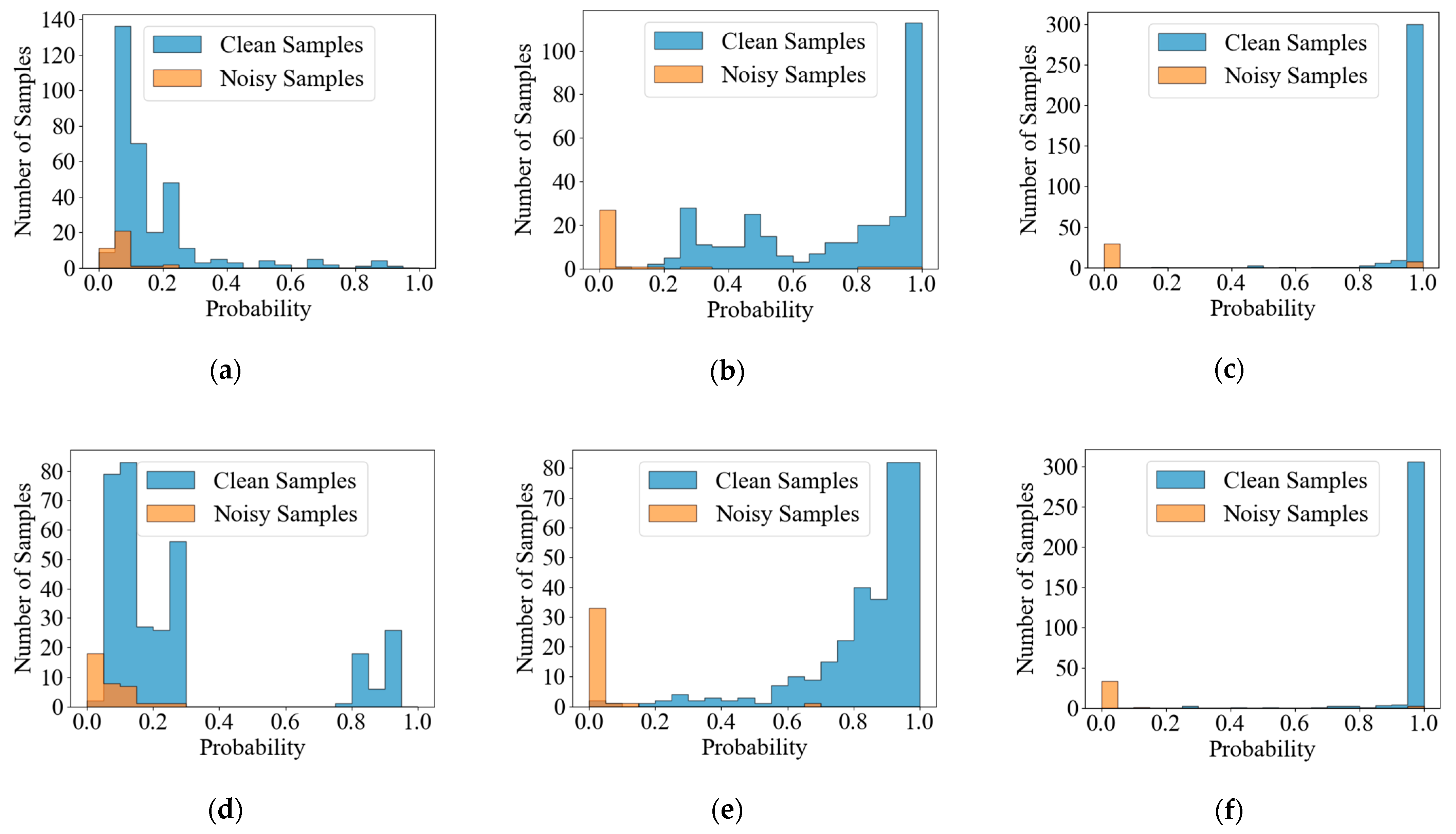
According to Equation (3), the value becomes smaller when the prediction probability of the complementary label is closer to 0. This increases the probability values of the other classes. In this way, the noisy radar jamming samples can be detected.
2.2. TR-Based Feature Extraction for Radar Jamming
Figure 2 shows the Transformer architecture in
Figure 1, which is the key part for extracting discriminative features of radar jamming. Given a radar jamming sample
with
sampling points, it is equally split into a series of non-overlapped pieces
. The series of non-overlapped pieces of radar jamming is defined as
where
indicates the size of a single piece. After linear projection, a trainable class token is appended to the piece tokens of radar jamming. Then, these tokens, along with their position information, form the initial input.
Next, the input is fed to the Transformer encoder for feature extraction, which consists of
Transformer encoder blocks. Specifically, one Transformer encoder block contains two layers of normalization, two element-wise addition operations, multi-head self-attention (
), and multi-layer perceptron. Note that the
is used for integrating long-range features of radar jamming, which can be formulated as follows:
where
.
,
are the query, key, and value, respectively.
, , and
are learnable weight matrices, and
=
and
represent the number of parallel attention heads.
Finally, the correlations between piece tokens of radar jamming are continuously aggregated into the class token from a global perspective. By following full connection, the predictions are created via a softmax function in the full connection layer.
2.3. Noisy Radar Jamming Sample Cleansing
Considering the fact that the model is prone to fit noisy labels, erroneous directions are provided when training the model. This leads to poor generalization performance. To address the aforementioned problem and further avoid memorizing the wrong information from noisy labels, the noisy radar jamming samples are removed in the proposed methods. Based on the assumption that the higher the predicted probability, the closer to the ground truth, the threshold
is used to filter out those radar jamming samples with noisy labels, as illustrated in
Figure 1. Let
denote the logits after softmax for the radar jamming sample
.
is the foundation for the predicted probability
, which can be formulated as follows:
where
denotes the true label of the radar jamming sample
.
points to the probability of the corresponding class of radar jamming sample
in row
of
.
Let
(
) represent the selected clean radar jamming training set, where
and
denotes the total number of selected clean radar jamming training samples. The clean radar jamming samples are defined as those with accurate labels. Meanwhile, the output probability
of radar jamming samples is compared with a set threshold
, which can be expressed as follows:
According to Equation (6), the original noisy radar jamming training set can first be estimated and divided into clean and noisy radar jamming training samples depending on the predictions and a threshold . Next, the judged clean and noisy radar jamming training samples are reserved and discarded, respectively. After that, the noisy radar jamming samples can be cleansed, and only the selected clean radar jamming training samples are used for the eventual recognition task. Noisy radar jamming sample cleansing is a useful tool to alleviate the negative impact caused by noisy radar jamming samples, resulting in better recognition performance.
2.4. Radar Jamming Recognition
After removing the noisy samples from the given noisy radar jamming training set , the selected clean radar jamming samples are fed into the feature extraction network to complement the recognition task. Two networks, the CNN and TR, are used to form RadarCL-CNN and RadarCL-TR, respectively. However, CNN has difficulty in modeling long-range dependencies because of the limitation of the convolutional kernel size. Compared with the CNN, the TR can capture distant relationships in radar jamming. According to the above analysis, the TR is more suitable for radar jamming recognition tasks.
All samples in are regarded as clean radar jamming training samples, whose labels are correct. Then, those radar jamming samples train the feature extraction network using the ordinary cross-entropy (CE) loss function.
Note that when minimizing the CE loss using the gradient descent algorithm, the closer the prediction probability of the true label is to 1, the smaller the value of loss (closer to 0), which is different from Equation (3).
Finally, the radar jamming testing set is fed into the trained feature extraction network to categorize each radar jamming sample into different groups based on their features and then generate recognition results.
3. The Proposed RadarSSL-PL-S-TR Framework for Radar Jamming Recognition with Labeled and Unlabeled Samples
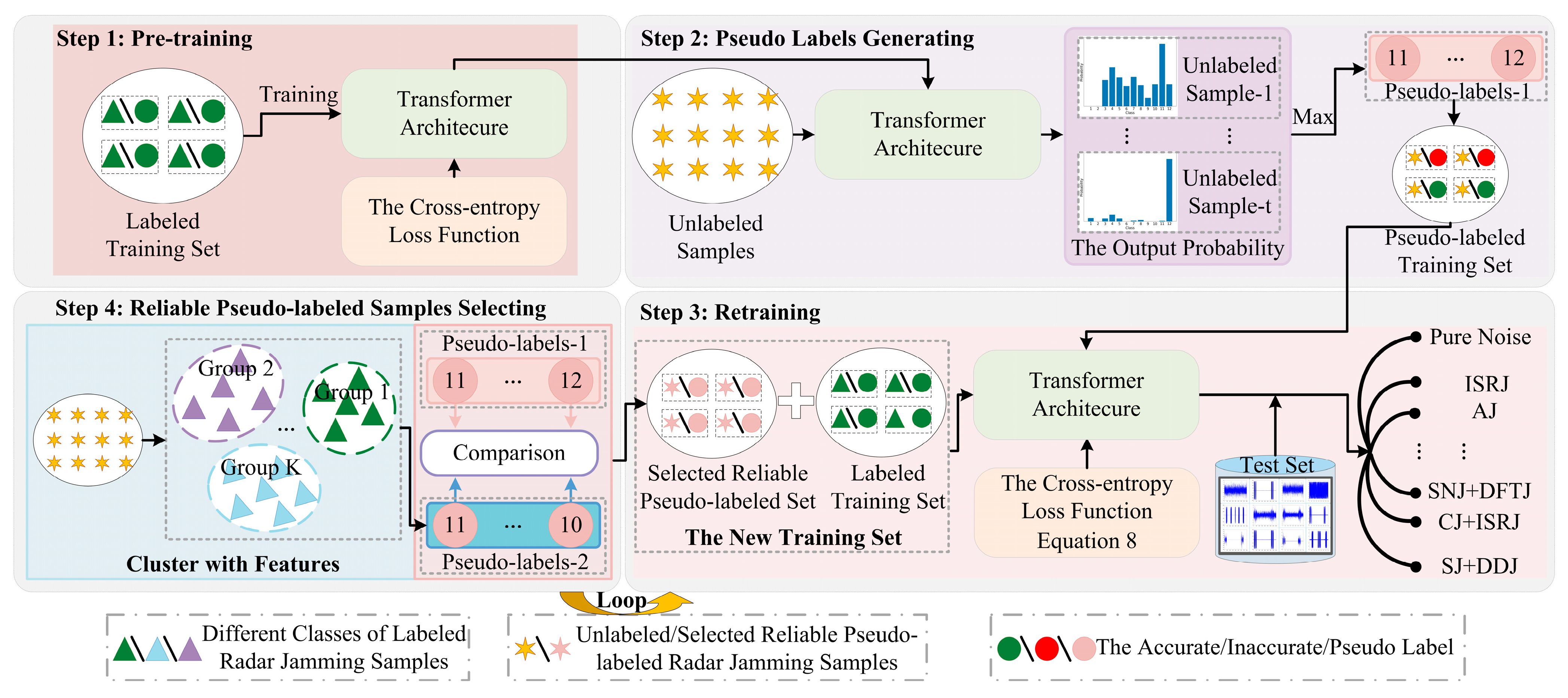
As shown in
Figure 3, the designed RadarSSL-PL-S-TR method consists of four main steps: pre-training with a labeled radar jamming set, generating pseudo labels for unlabeled radar jamming samples, retraining with a labeled and pseudo-labeling radar jamming set, selecting reliable pseudo-labeling radar jamming samples, and then looping back to step 3. First, labeled radar jamming samples are used to pre-train the feature extraction network to provide a foundation for obtaining the pseudo labels of unlabeled samples. Next, the unlabeled radar jamming samples are sent to the trained model in step 1 to generate pseudo labels. Then, the pseudo-labeling and labeled radar jamming samples are combined to train the recognizer. Finally, the reliable pseudo-labeling radar jamming samples are regarded as labeled samples and added to the original label set to form the new labeled radar jamming training set. Meanwhile, step 3 and step 4 loop.
3.1. Pre-training Labeled Radar Jamming Set
Due to the challenge of radar jamming sample labeling in practical applications, there may be a large amount of unlabeled samples but few labeled samples in the radar jamming dataset. In general, the number of labeled radar jamming samples has a great impact on the recognition performance, and the recognition performance will be heavily hampered by only using a few labeled radar jamming samples to train the network. To overcome the issue of recognition performance degradation under limited labeled radar jamming samples, unlabeled radar jamming samples should be fully utilized during the training process with the aim of achieving better recognition performance.
Let
and
(
) denote the labeled radar jamming training set with
labeled radar jamming samples and
unlabeled radar jamming samples, respectively. As shown in
Figure 3, step 1 aims to optimize the deep feature extraction model with labeled radar jamming samples using CE loss. After that, the unlabeled radar jamming samples are matched to their corresponding pseudo labels by reusing a trained model.
3.2. Generating Pseudo Labels for Unlabeled Radar Jamming Samples
Note that the connection between labeled and unlabeled radar jamming samples can be established by relying on the feature representation space in a trained model (defined as
). In this way, pseudo labels are assigned to unlabeled radar jamming samples via the model itself. Specifically, for an unlabeled radar jamming sample
, followed by feeding
to
, a series of predicted probabilities under different classes are output. Then, the category corresponding to the maximum predictions is regarded as the pseudo label for a given unlabeled radar jamming sample, which can be written as follows:
where
represents pseudo labels for unlabeled radar jamming samples
, and each
in
is composed of the highest predicted probability. In this way, the pseudo-labeling radar jamming training set is created as
.
Pseudo labels provide a way to make use of these unlabeled radar jamming samples, which enables recognition performance to be improved by learning from both labeled and unlabeled radar jamming samples with pseudo labels instead of only learning from a few labeled radar jamming samples. Training the model via a large amount of unlabeled radar jamming samples with the generated pseudo labels can significantly promote the generalization ability of the model.
3.3. Retraining Labeled and Pseudo-Labeling Radar Jamming Set
The model gains prediction ability from learning the labeled radar jamming samples and applies it to produce pseudo labels for unlabeled radar jamming samples. Once the pseudo labels are obtained, the unlabeled radar jamming samples can participate in training a network, which is helpful in capturing richer and more discriminative features of radar jamming, that is, both the labeled radar jamming training set
and pseudo-labeling radar jamming training set
are employed to facilitate the training process. In particular, taking the loss function of pseudo-labeling samples into consideration, the overall loss function combining the loss functions of labeled and pseudo-labeling radar jamming samples can be computed as follows:
where
and
are the losses for labeled and unlabeled radar jamming samples with pseudo labels, respectively.
is the CE loss function.
is a hyperparameter, which indicates the weight
of pseudo-labeling radar jamming samples and changes with epoch.
and
represent the
epoch and the total number of epochs, respectively.
3.4. Selecting Reliable Pseudo-Labeling Radar Jamming Samples
Despite the pseudo labels being generated based on the model’s high-confidence predictions, the generated pseudo labels are sometimes inaccurate. To mitigate the misguidance of incorrect pseudo labels to the model, it is necessary to select unlabeled radar jamming samples with reliable pseudo labels.
A simple yet effective method is used to select high-quality pseudo labels. Specifically, first, the clustering algorithm, i.e., the approximate rank-order clustering (AROC) algorithm, is adopted to generate pseudo labels based on the assumption that radar jamming samples belonging to the same group tend to possess the same label. Then, each given unlabeled radar jamming sample in can acquire its pseudo label according to the AROC cluster with labeled radar jamming samples, which are defined as . The pseudo labels of and are compared element by element, and then the pseudo-labeling radar jamming samples are split into reliable and unreliable pseudo-labeling radar jamming samples. In general, the pseudo labels are regarded as reliable labels when they are the same in both and . Otherwise, the pseudo labels are considered unreliable.
Next, according to the comparison results, the selected reliable pseudo-labeling radar jamming set is denoted as . Then, the unlabeled radar jamming samples with reliable and unreliable labels are added to the labeled radar jamming training set and pseudo-labeling radar jamming training set, respectively. In this way, a labeled radar jamming training set and pseudo-labeling radar jamming training set are updated and redefined as and , respectively. The radar jamming recognition performance is gradually improved via iterating step 3 and step 4.
4. Datasets and Experimental Settings
4.1. Data Description
The radar jamming simulation dataset is used to verify the effectiveness of the proposed methods. In the dataset, linear frequency modulation (LFM) signal is used as the radar transmission waveform, which can be described as follows:
where
is the frequency modulation slope.
is the bandwidth, and
denotes the pulse width. Their values are
and
, respectively. The
can be expressed as follows:
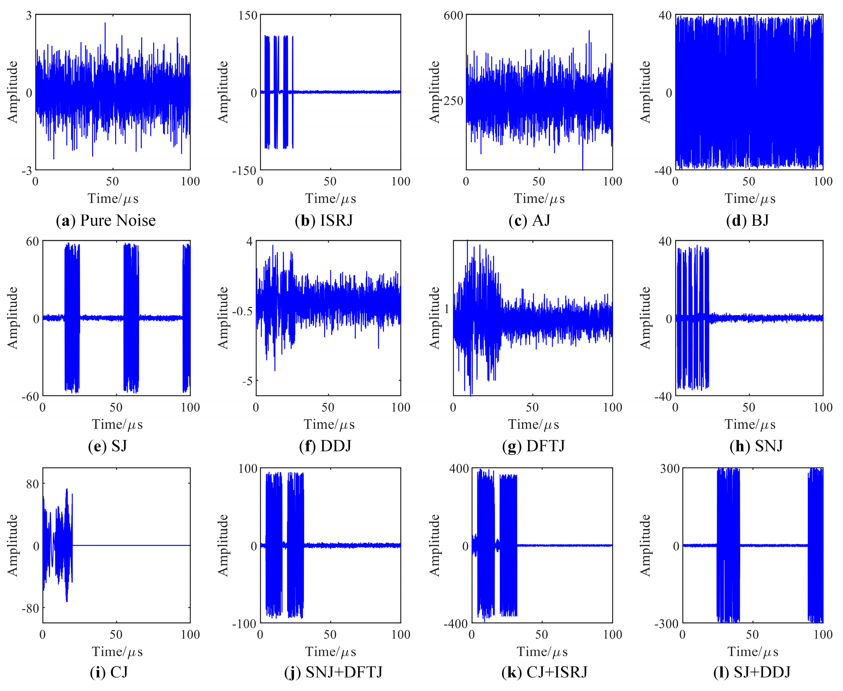
According to the different jamming effects, the radar jamming simulation dataset can be divided into pure noise, suppression jamming (i.e., aiming jamming (AJ), blocking jamming (BJ), and sweep jamming (SJ)), deception jamming (i.e., distance deception jamming (DDJ) and dense false target jamming (DFTJ)), novel jamming (i.e., interrupted-sampling repeater jamming (ISRJ) and smart noise jamming (SNJ)), passive jamming (i.e., chaff jamming (CJ)), and compound jamming. In summary, 12 types of radar jamming signals (i.e., the value of
is 12) are created, with each containing 500 samples, making a total of 6000 samples (i.e., the value of
is 6000).
Figure 4 shows their time domain waveforms, where the 12 types of radar jamming signals can be labeled sequentially as C1 to C12.
The sampling rate is , and the pulse repetition interval (PRI) is 100 . Consequently, each sample has 2000 complex sampling points. Then, the real and imaginary part of the complex sampling points are concatenated. This means each sample has 4000 sampling points (i.e., the value of is 4000), and the former and the latter 2000 points correspond to the real part and the imaginary part, respectively. At the same time, the piece size is set to 16.
- (1)
Aiming Jamming (AJ)
Compared to the other types of radar jamming, the bandwidth of AJ is narrow. It is randomly set to
times the LFM signal bandwidth
(i.e.,
). AJ is usually used with noise amplitude modulation jamming, which can be expressed as follows:
where
is the direct current bias. The modulation noise
is a generalized stationary random process distributed in the interval
with a mean of 0.
is a random variable uniformly distributed over the interval
and independent of the modulation noise
.
- (2)
Blocking Jamming (BJ)
BJ can be generated quickly. It requires the jammer to have a higher power. It is randomly set to
times the LFM signal bandwidth (i.e.,
). BJ is usually used with the noise frequency modulation jamming, which can be expressed as follows:
where
and
are the amplitude and the frequency modulation slope of noise frequency modulation jamming.
- (3)
Sweep Jamming (SJ)
The principle of SJ is the same as that of BJ, except the bandwidth range is larger and changes periodically. When the bandwidth of jamming exceeds the bandwidth of the receiver, the receiver cannot receive the jamming signal, so there will not be jamming in the position where the jamming bandwidth is greater than the bandwidth of the receiver.
It can be observed in
Figure 4e that the amplitude of the noise frequency modulation in SJ is constant within the bandwidth of the radar receiver, and the frequency is LFM superimposed with a random frequency.
- (4)
Distance Deception Jamming (DDJ)
DDJ intercepts radar signals and then forwards them after modulation. To achieve the effect of deception as much as possible, only the time delay and the amplitude are modulated, so the forwarded jamming signal is similar to the radar signal waveform. Specifically,
where
is the amplitude of DDJ.
denotes the time delay corresponding to the target echo, and
represents the additional time delay of jammer forwarding. The jamming amplitude
varies randomly from
to
. The time delay of DDJ is randomly selected from
to
.
- (5)
Dense False Target Jamming (DFTJ)
Unlike DDJ, which forwards one false target, DFTJ forwards multiple false targets. It can be expressed as follows:
where
is the number of forwarded false targets, and its value is set to
. Additionally, the time delays of the target and the
f-th false target are denoted as
and
, respectively.
is the amplitude of the
f-th false target.
- (6)
Interrupted-Sampling Repeater Jamming (ISRJ)
ISRJ captures part of target signals and repeatedly forwards them. After that, false targets are created, which harm the performance of radar systems. The time-domain expression for ISRJ is expressed as follows:
where
and
are the amplitude and number of repeated forwarding processes, respectively.
denotes the time delay of the ISRJ.
is the radar signal and is defined in Equation (9).
and
are the sampling duration and the convolution, respectively.
and
represent the PRI and its number.
- (7)
Smart Noise Jamming (SNJ)
The sampling and forwarding modes of SNJ are similar to those of ISRJ, and they all belong to novel radar jamming. The Gauss white noise
is adopted to generate SNJ, which can be expressed as follows:
- (8)
Chaff Jamming (CJ)
Radar active jamming can destroy the function of acquiring target information in the background of strong jamming by actively transmitting high-power electromagnetic radiation signals. This active jamming method also has some hidden dangers, and the active jamming signal will also become the target of the enemy’s counter-confrontation and attack. In addition to active jamming, passive jamming methods can also be used to produce deception and suppress jamming effects. CJ is a kind of passive jamming that is commonly used, which can be expressed as follows:
where
is the number of chaffs in chaff clouds. Its value is randomly selected from the range of
to
.
is the Doppler shift of the
i-th chaff. The Doppler frequency shift caused by chaff cloud translation is
. The Doppler variance of a single chaff is
.
- (9)
Compound Jamming
In the complex battlefield environment, the cooperative operation of multiple jammers not only makes the radar receive single jamming but also additive compound jamming containing two or more jamming signals. Therefore, this article combines the above process of single radar jamming to obtain three-compound jamming: DFTJ + SNJ, CJ + ISRJ, and DDJ + SJ.
The JNR of AJ, BJ, SJ, ISRJ, and SNJ is randomly selected in the interval , where JNR represents the ratio of jamming to signal.
4.2. Evaluation Metrics
To evaluate recognition performance, two widely used quantitative metrics (i.e., the overall accuracy and kappa coefficient ) in recognition tasks are employed. Higher values of the two above quantitative metrics indicate better recognition performance of the method. The average per-class accuracy is defined as the mean accuracy for each type of radar jamming. Furthermore, to mitigate the impact of random errors and guarantee the reliability of the recognition results, the results are reported in the form of the mean and standard variance with five independent experiments.
is the proportion of correctly recognized test samples
among the total number of test samples
, which is defined as
quantifies the consistency between the model-predicted outcomes and actual results, defined as
where
and
are the number of actual test samples per class and the number of predicted test samples per class, respectively.
is the total number of classes.
4.3. Experimental Setup
- (1)
Experimental Setup for Recognition with Noisy-Labeled Samples
For recognition with noisy-labeled samples, in each class, 30 samples and another 3 samples are randomly chosen as the training set and the validation set, respectively, and the rest of the samples are used as the testing set. The widely used advanced methods based on noise-robust loss functions, including generalized cross entropy (GCE) [
39] and symmetric cross entropy (SCE) [
40], are used as comparison methods. The hyperparameter q in [
39] is set to 0.5. In [
40], the hyperparameters alpha and beta are set to 0.1 and 1.0, respectively.
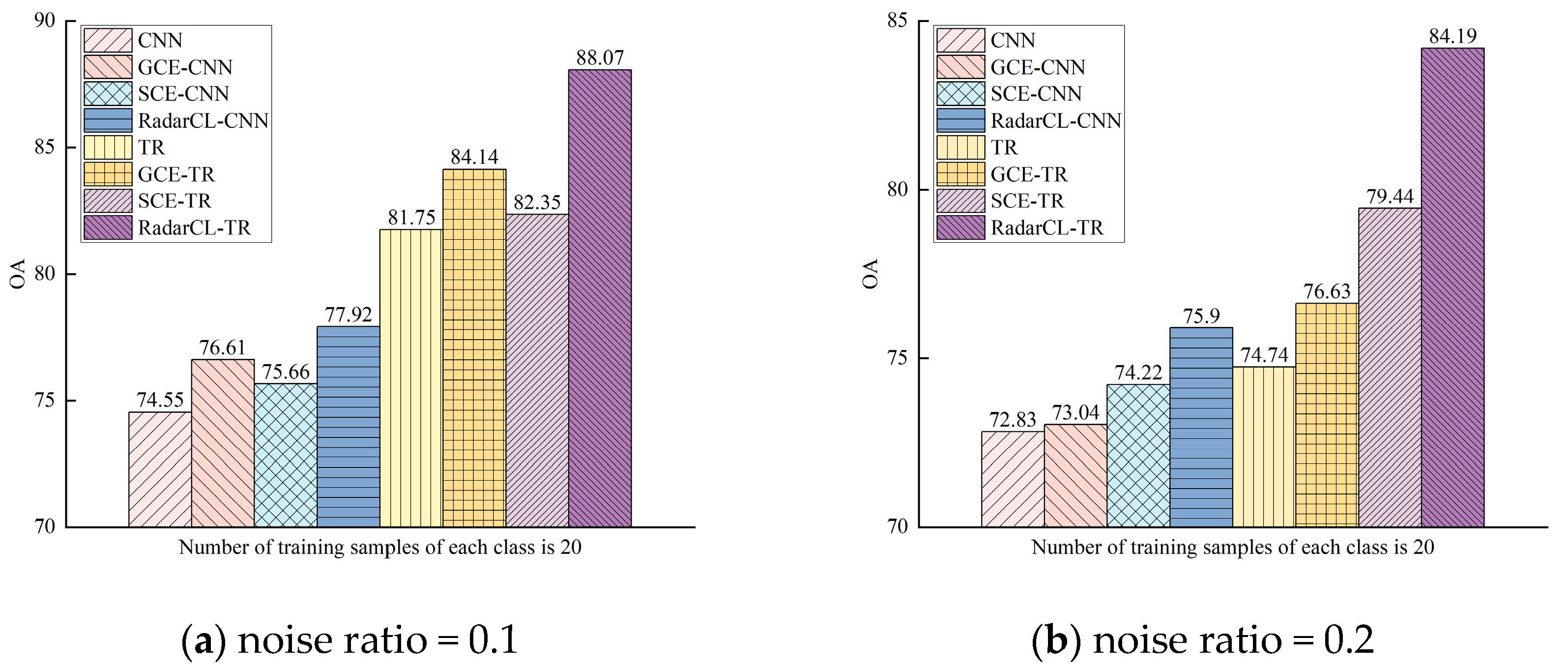
In the following experiments, the symmetric noise ratios are set to 0.1 and 0.2 to compare the performance of different methods. The results are reported as the mean and standard variation obtained from ten independent runs using randomly selected training samples in each run.
For the proposed RadarCL-TR methods, the number of Transformer encoder blocks and parallel attention heads are set to 5 and 6, respectively. During the training process, the initial learning rate in the first stage of noisy radar jamming sample detection is set to 0.0009. Considering the difference in the output probability between noisy and clean samples, the threshold α is set to 0.5 in the second stage. Additionally, a learning rate adjustment method using cosine annealing from 0.001 to 0.0001 is adopted in the last radar jamming recognition stage.
- (2)
Experimental Setup for Recognition with Labeled and Unlabeled Samples
For recognition with unlabeled samples, 10 training samples (denoted as
and
) for each class are selected as the labeled training set to explore the recognition performance of different methods. The proposed RadarSSL-PL-S-TR is compared with popular semi-supervised recognition methods, such as label propagation (LP) [
41] and Laplacian support vector machine (LapSVM) [
42].
For the proposed RadarSSL-PL-S-TR, the initial learning rate and epochs in the pre-training stage are set to 0.001 and 100, respectively. The learning rate and epochs in the retraining stage are set to 0.00007 and 50, respectively.
To guarantee a fair comparison, all experiments are conducted on NVIDIA GeForce RTX 3060.
6. Conclusions
In this paper, first, the idea of complementary label learning was explored for radar jamming recognition with noisy labels. The proposed RadarCL-TR methods were found to be effective for radar jamming recognition in the presence of noisy samples. More specifically, by learning from complementary labels, the proposed RadarCL-based methods, including RadarCL-CNN and RadarCL-TR, reduced the negative impact on recognition accuracy and obtained the highest accuracy in CNN-based methods and TR-based methods, respectively. Moreover, owing to the superior ability to capture global dependencies of radar jamming, RadarCL-TR increased the by and compared to RadarCL-CNN at the noise ratios of 0.1 and 0.2, respectively.
Next, to address the issue of poor radar jamming recognition performance with few labeled samples but plenty of unlabeled samples, RadarSSL-PL-TR was investigated. In detail, RadarSSL-PL-TR adopted pseudo labels to utilize unlabeled radar jamming samples, thereby increasing the number of training samples. Simultaneously, the long-range dependencies were well captured using the TR. Thus, the radar jamming recognition performance was significantly improved under conditions with plenty of unlabeled samples. Furthermore, a selection module was designed to select reliable pseudo-labeled samples, which was helpful in capturing more distinctive features. Hence, RadarSSL-PL-S-TR showed an improvement of in the compared to RadarSSL-PL-TR.
This research has opened a new door for further studies to explore weakly supervised radar jamming processing.


