Abstract
The past decade has seen remarkable advancements in Earth observation satellite technologies, leading to an unprecedented level of detail in satellite imagery, with ground resolutions nearing an impressive 30 cm. This progress has significantly broadened the scope of satellite imagery utilization across various domains that were traditionally reliant on aerial data. Our ultimate goal is to leverage this high-resolution satellite imagery to classify land use types and derive soil permeability maps by attributing permeability values to the different types of classified soil. Specifically, we aim to develop an object-based classification algorithm using fuzzy logic techniques to describe the different classes relevant to soil permeability by analyzing different test areas, and once a complete method has been developed, apply it to the entire image of Pavia. In this study area, a logical scheme was developed to classify the field classes, cultivated and uncultivated, and distinguish them from large industrial buildings, which, due to their radiometric similarity, can be classified incorrectly, especially with uncultivated fields. Validation of the classification results against ground truth data, produced by an operator manually classifying part of the image, yielded an impressive overall accuracy of 95.32%.
Keywords:
remote sensing; OBIA; WorldView-3; satellite imagery; land use classification; fuzzy logic 1. Introduction
The earth observation (EO) sector has seen notable technological progress in recent years, especially in the satellite sector, where increasingly higher-resolution images have been put on the market. Satellite resolutions rapidly went from values lower than one meter, for example, the SPOT 6 and 7 satellites with a Ground Sample Distance (GSD) of 1.5 m on the ground in the panchromatic image, defined as medium–high resolution. Up to a GSD of 31 cm, like those of the acquisitions of the WorldView-3 and WorldView-4 satellites, or more generally, acquisitions below one meter always refer to the panchromatic image, defined as having very high resolution. In addition to the very high resolution, these products are available with return times, i.e., the possibility of having an image of the same area of the planet in less than a week in some cases. All these advances have attracted more and more interest in the development of methodologies for soil classification, more or less automated, aimed at facilitating many applications, from the creation of maps to various uses in precision agriculture, monitoring the health of crops, to the observation of cities and their development. Thanks to the very short revisit times, the monitoring of an area by applying change detection techniques to the images is increasingly used even in the most extreme situations, in which, following natural disasters, it can provide support in estimating the damage and planning the necessary interventions to restore the territory [1]. Our world is changing more and more rapidly, and satellite images have definitively become a valid tool for promptly observing and monitoring this change. At the same time, increasingly high-performance classification methodologies have been developed, from pixel-based analysis to object-based analysis (OBIA), deep learning algorithms, and, although computationally more expensive, convolutional neural networks (CNNs) have become more popular in recent years. The state of the art sees the use of such algorithms and methods for most applications, not only in the classification of the scene in terms of land use but also in the previous phases, such as image fusion, segmentation, and registration of images. These methods, although very effective, must be some more, some less trained in some way to perform their function for the classification of land use by providing known image elements, elements already classified that are sometimes not available in large quantities. In the work presented below, an object-based approach combined with the use of fuzzy logic is proposed; radiometric and geometric aspects of the objects segmented in the image are used simultaneously in a logical scheme designed to reproduce what could be the line of thought of a human observer looking at the image. In this way, the training phase is eliminated, which, while maintaining the logical descriptive scheme of the class, is currently replaced by the calibration of the parameters, which, applied to the individual membership functions, duly combined with each other, define the class of an object. Mainly, the proposed method has the advantage of exploiting a logical description of the classes, which, once defined, is not strictly linked to the context analyzed, but precisely because it is developed on the basis of what could be the considerations of a human observer, it has greater versatility. In addition to this, you do not need to sacrifice for training, if present, part of the ground truth; this phase is replaced by a necessary calibration of the parameters that describe the various classes. However, it must be taken into consideration that this operation does not require much time, as the geometric parameters can be easily adapted depending on the resolution of the image available. Radiometrically, the description of the classes and the main factors involved are the indices and the standard deviation; the indices already have normalized values and are therefore suitable in contexts like the one analyzed, while the standard deviation values can be adjusted in various attempts or by evaluating the correlation with the histograms of the image bands, with images already classified. The ultimate objective of our work is to obtain a soil permeability map, attributing permeability values to the identified classes, through a classification method accurate enough that we need the ground truth only for what is strictly necessary to validate the results since, if not already available, creating ground truth is a very time-consuming activity. In this work, a step forward has been made, using a portion of the Pavia image, for the development of the logical scheme to identify the class of fields and to test the logical scheme describing the water class developed in previous work to effectively distinguish it from the shadows in an urban context, a problem well known in the literature [2]. In both works, the image used is the same, but different areas were analyzed; specifically, the image was acquired by the WorldView3 satellite [3] in March 2021 over the entire area of the municipality of Pavia, a city located in Italy in the Po Valley. It has the ability to acquire a panchromatic image at a ground resolution of 30 cm with a revisit frequency of 4.5 days at 20° off-nadir or less. The raw data are composed of a panchromatic band with a GSD of 31 cm and eight multispectral bands: Coastal Blue, Blue, Green, Yellow, Red, Red Edge, Nir1, Nir2, with a GSD of 124 cm. From these, by carrying out a pansharpening operation based on the Gram–Schmidt orthogonalization [4], using the ArcGIS Pro software, it was possible to analyze and classify an image with a GSD of 31 cm and an estimation of the spectral information of the eight bands. The developed algorithm is mainly composed of three phases: segmentation, classification, and refinement; the result is then compared with the ground truth created specifically in our laboratory by an operator, who patiently identified and manually classified a good number of objects before the classification had been performed. The area manually classified to constitute the ground truth is equal to 975.092,3 square meters, or 15.64% of the analyzed area. The result obtained satisfied us because, beyond the overall accuracy value achieved, 95.32% is already very good in itself. Given the heterogeneity of the scene, it makes us think we can proceed with the classification of the entire image in our possession, keeping the methodology and parameters used unchanged and obtaining a good result. Tests carried out on other portions of the image do not reveal any particular limitations related to the method and seem to confirm its effectiveness, at least visually, by returning a good classification. However, at the moment, we do not have the possibility of rigorously showing its effectiveness in terms of accuracy as we do not have sufficient truth to the ground in those areas.
2. Materials and Methods
The area analyzed is a portion of the image acquired by the WorldView3 satellite in March 2021 of the entire municipal area of the city of Pavia. The product purchased from the Geomatics Laboratory of the University of Pavia includes for the entire area an 8-band multispectral image with a lower ground resolution, equal to approximately 120 cm for each pixel, and a panchromatic image, which, in a gray scale, shows the entire area with a ground resolution of approximately 30 cm, as summarized in Figure 1. In addition to the panchromatic and multispectral components, the WorldView3 satellite is capable of acquiring another 8 short-band infrared (SWIR) bands, which have an even lower resolution of approximately 320 cm on the ground [3]. The SWIR component of the image was not purchased because we are interested in seeing what can be obtained from a high-resolution image, and the data resulting from this component have a high but not sufficient spatial resolution. For this reason, only the panchromatic and multispectral components of the image of the Pavia area were purchased and used for classification.
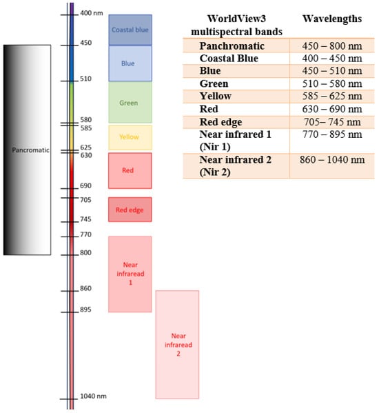
Figure 1.
This diagram represents the bands captured by the multispectral sensor of the WorldView3 satellite with the relative wavelength intervals.
The two components, panchromatic and multispectral, were combined by applying the pansharpening algorithm based on Gram–Schmidt orthogonalization [5]. Within ESRI’s ArcGIS ProTM v.3.0.2 software, the details of the technique used by the software are described in this patent [6], obtaining an image with the spectral information of the 8 bands (Coastal Blue, Blue, Green, Yellow, Red, Red Edge, Nir 1, Nir 2, and the degree of detail of the panchromatic image) at an almost 30 cm resolution on the ground [4]. Clearly, the result obtained, distorts the basic multispectral information; various algorithms could have been explored to enhance the image quality and minimize spectral errors [7]. The achieved level of detail, even without additional algorithms, is noteworthy. This detail proves crucial for distinguishing diverse elements within the urban area. However, the advantage of working on a much more detailed image is that it allows a significantly higher degree of accuracy to be achieved for classification purposes.
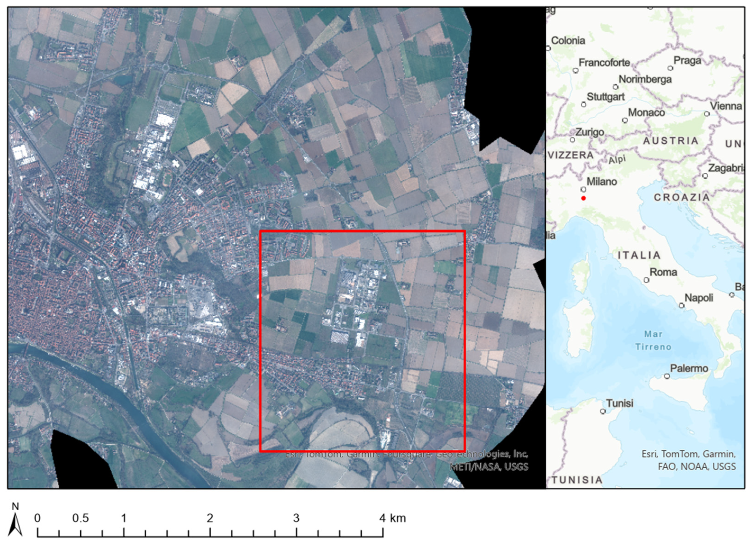
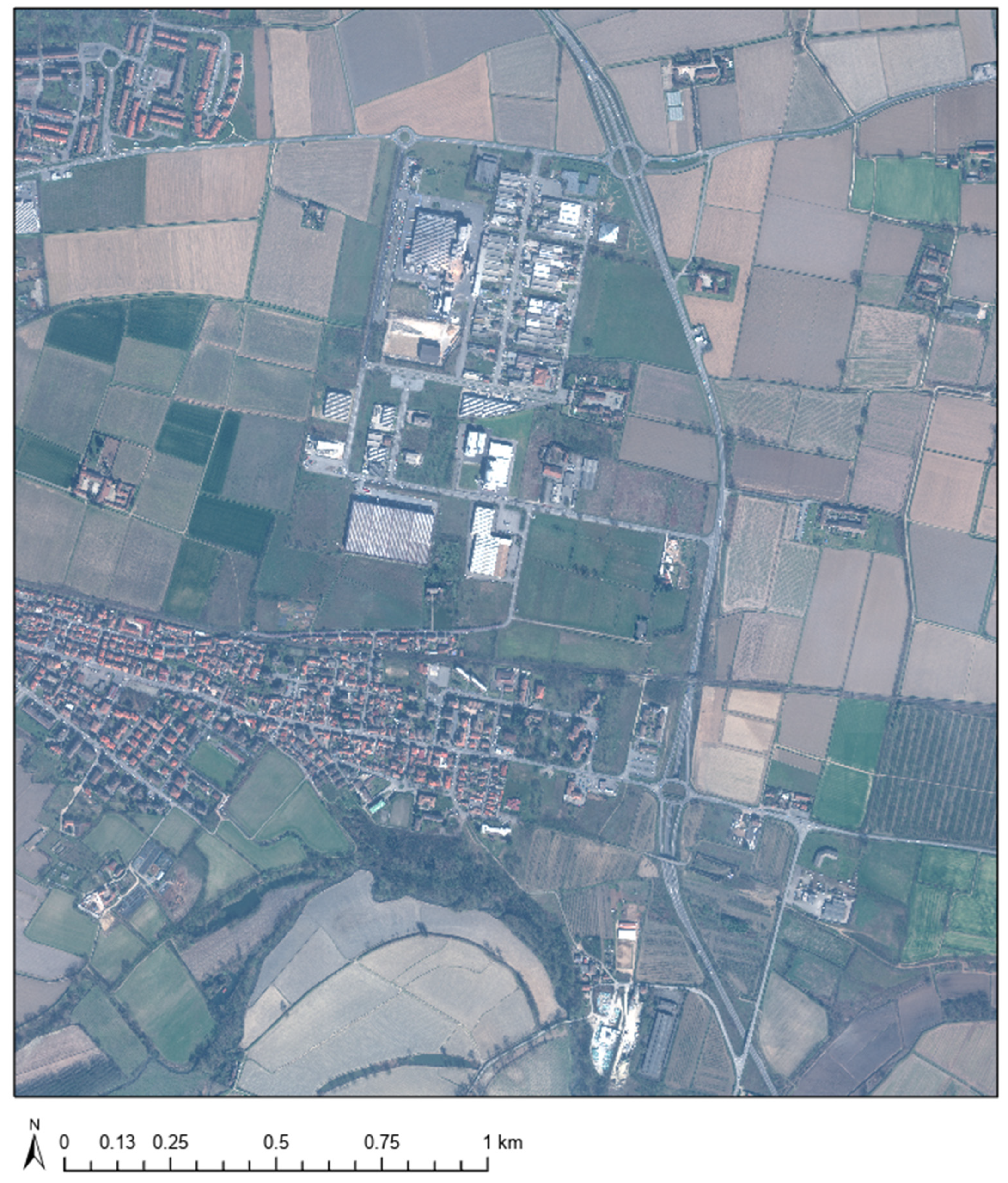
The area analyzed is located slightly east of the historic center of the city, as shown in Figure 2, and features a modest-sized industrial area and small residential areas; the rest is made up of agricultural areas and isolated farms. The choice was influenced by the fact that this area involves various elements, in particular large industrial buildings, which in past classifications were sometimes erroneously classified as uncultivated fields, small lakes and waterways, and isolated buildings in the middle of the countryside, all located in an area adjacent to the residential center (see Figure 3). This proximity allows us to see if the algorithm and the methodology developed are suitable for dealing with a mixed context and, therefore, applicable to the entire image without having to modify the parameters specifically. This occurs through a dedicated segmentation process, using the multiresolution segmentation algorithm [8], set in a first phase to identify very large objects, the size of fields, and after having identified them as fields or not, a detailed segmentation is necessary to continue in image classification. Both in the segmentation and classification phases, two indices are exploited: the Normalized Difference Vegetation Index (NDVI) [9] and the Normalized Difference Water Index (NDWI) [10], which are very useful for highlighting and, therefore, more easily identifying vegetation and water, respectively. The result obtained from the classification is ten refined using algorithms that allow the fusion of adjacent objects if they satisfy certain criteria and algorithms that allow the classified objects to grow in neighboring pixels under certain conditions, which are exceptionally effective for improving the edges of objects classified as water. Overall, the area studied is composed of 64,877,220 pixels and covers an area of 5.8389 square kilometers. In the area, there are no large watercourses, only small streams and lakes, which are identifiable during the construction of the ground truth in some cases only because the trees above them do not yet have fully developed foliage in early spring. Approximately half of the fields present have crops in an advanced state, while others have either recently passed the sowing phase or have still been left in an uncultivated state, depending on the type of harvest. Paradoxically, we will see in the next chapters how some small wooded areas will be classified as uncultivated fields precisely because the foliage of the trees is not yet developed and no other vegetation has grown on the ground because it is covered by dead leaves.

Figure 2.
Pavia is a city in northern Italy, located south of the city of Milan. The area studied in this work, highlighted in red, is located just outside the city center towards the east.

Figure 3.
The studied area is characterized by a modest industrial area surrounded mainly by land for agricultural use, except for a small urban area present in the upper right corner of the image and another just below the industrial area.
The methodology applied is basically the same as already presented in a previous article [2] where the approach used for the classification of urban land was exposed. Focusing mainly on the correct distinction during the classification phase between shadows and water is a well-known problem in the literature [11,12,13,14], during the classification of urban areas. The main steps have remained unchanged, and in the order, the useful indices are first calculated, then a first segmentation is carried out to identify and subsequently classify larger objects such as fields, and a second segmentation to identify and classify smaller objects, water, and vegetation. Finally, the classified objects are refined to better define their edges, and what has not yet been classified is attributed to the impermeable class. Even if some parameters have been slightly adapted during the segmentation phase, the main feature remains unchanged, namely the creation of a logical scheme that exploits both the geometric and spectral characteristics of the segmented objects. A scheme is derived on the basis of what could be the logical processes that a human observer could generally adopt to distinguish the various elements in the image.
2.1. Index Calculations
In this first phase, the indices that can be useful in the classification phase are added to the radiometric information; in our case, the only indices that are calculated are NDWI (Normalized Difference Water Index) [10,15] and NDVI (Normalized Difference Vegetation Index) [16,17]. These two indices are among the best known in the literature and are often used in different fields, not necessarily just the classification of water and vegetation [9].
These new “bands” were not only used to identify the various classes more easily but directly in the segmentation phase, where they contributed to better identifying the edges of objects that could mainly belong to the water and vegetation classes. As indicated in the formulas above, only the Nir2 band is used in the index calculation because, compared to the Nir1, it presents higher values, generating higher index values compared to what was calculated with the Nir1. Compared to the other bands involved in the segmentation, the indices will have a greater weight as the information that can be extracted depends greatly on the near-infrared values, both for the identification of water bodies and green areas, for which the soil permeability values are significantly different from man-made structures.
2.2. Segmentation
Among the various segmentation algorithms present within the eCognitionTM v. 10.3 software, we have chosen to use the algorithm called multiresolution segmentation [8] both for the first phase of identification and classification of fields and for the second phase of identification and classification of smaller objects. This algorithm proceeds to merge individual pixels into objects based on mutual similarity at the spectral level; the user can adjust this similarity by specifying a scale factor that manages the heterogeneity of the objects; high values of this factor will lead to the identification of larger objects and therefore more radiometrically heterogeneous objects. The user can indicate the bands to take into consideration during this process and the different weights for each band. In addition to this, the objects can be different depending on the shape factor entered by the user; this value can vary from 0 to 1 and influences how much the shape of objects should be considered at the expense of the weight of the spectral information.
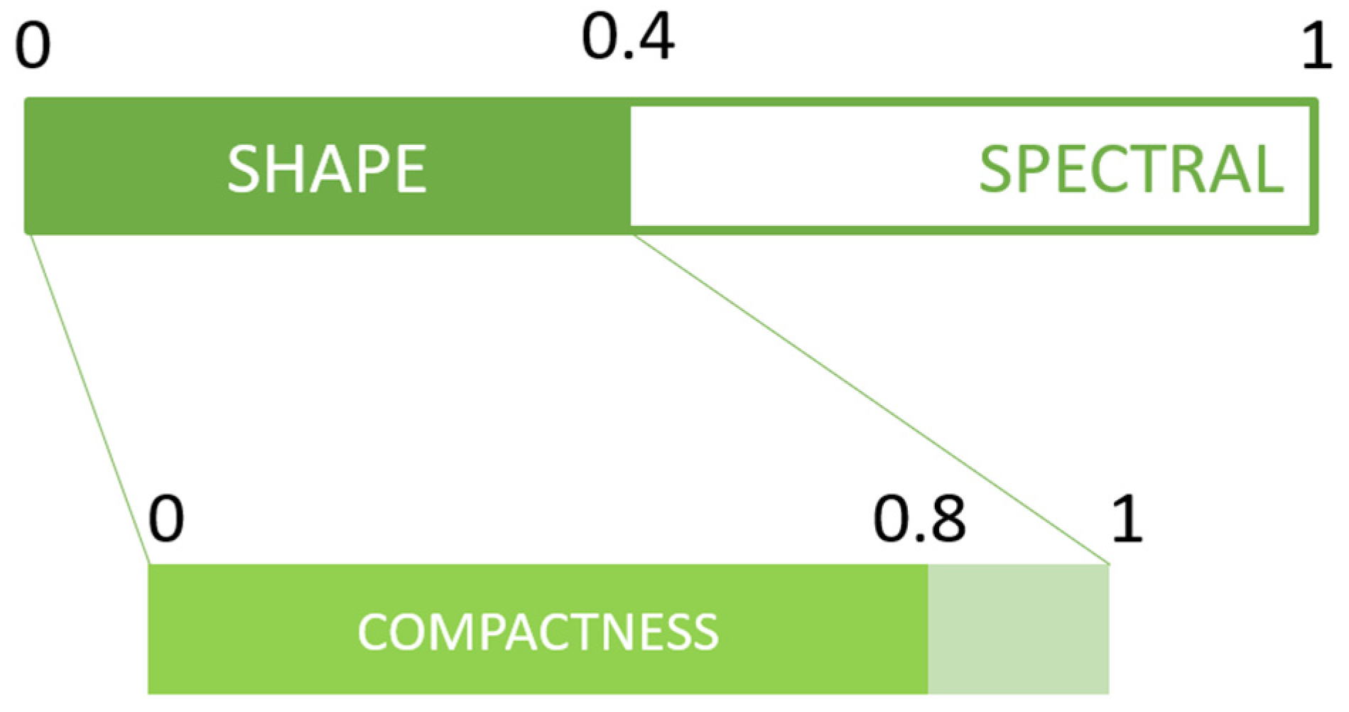
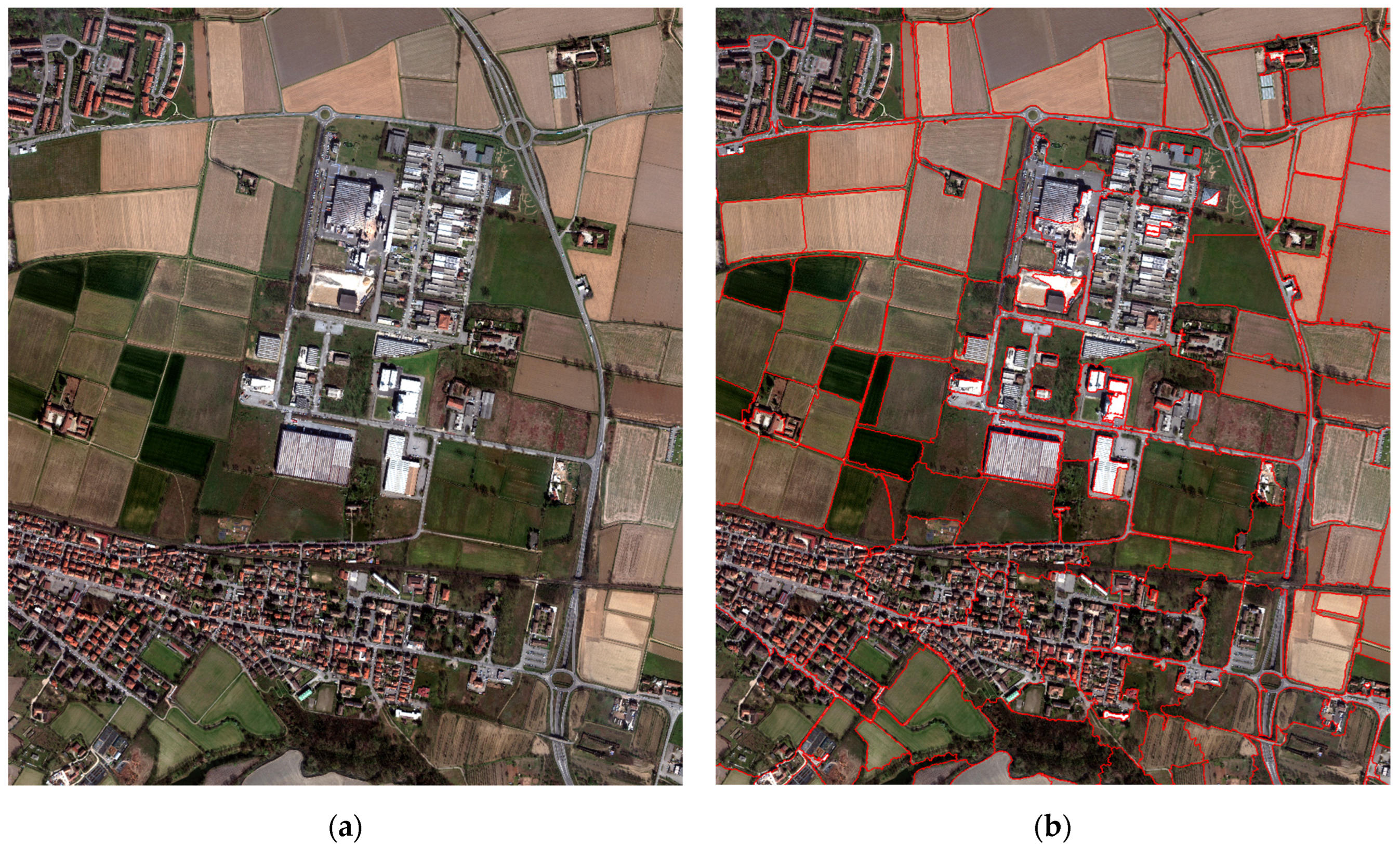
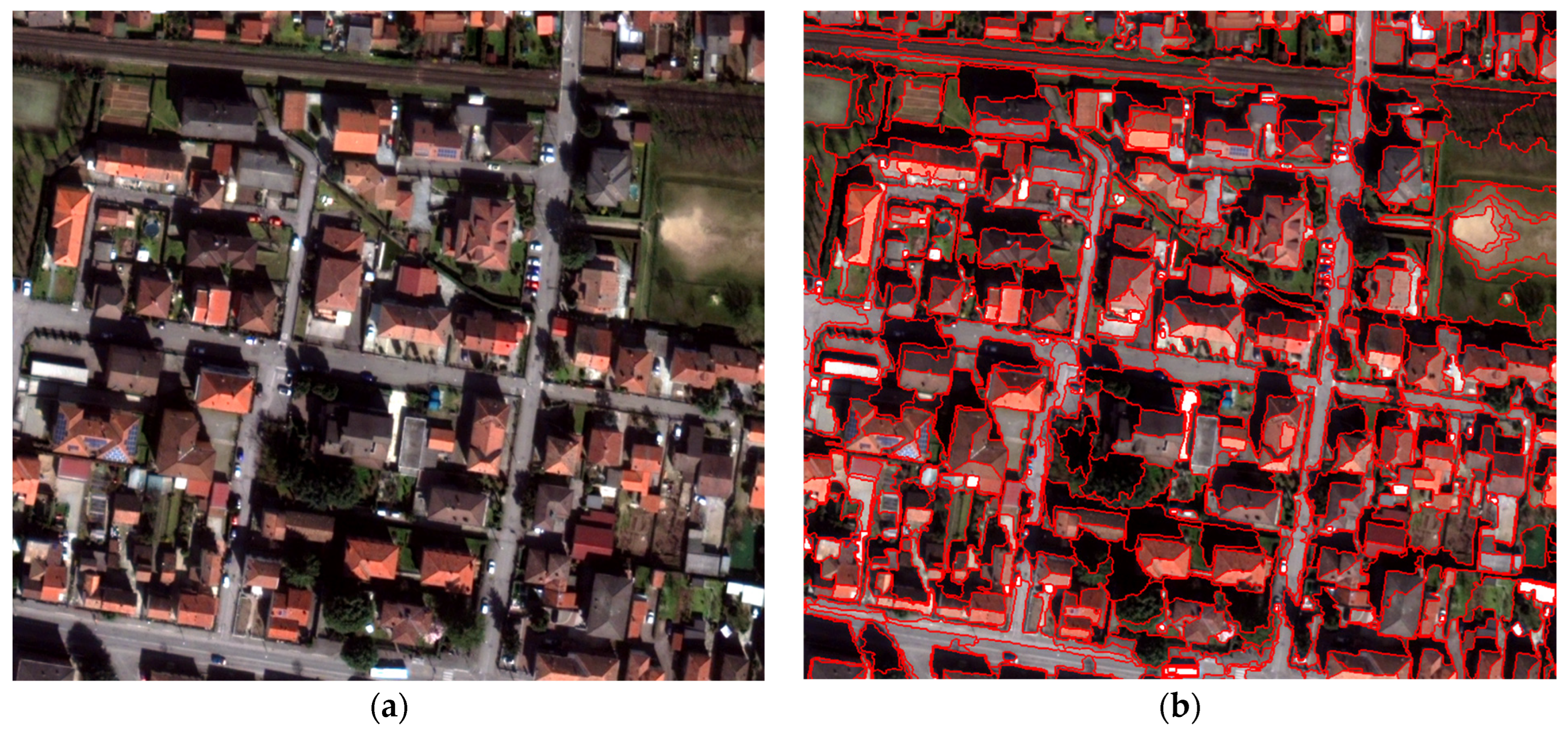
Similarly, the shape of objects is influenced by a further factor called compactness, which can also take on values compressed between 0 and 1. Knowing that the interaction of these factors with each other can be complex to interpret, two diagrams are shown below in which the values attributed to each factor and their relationship for both classifications carried out are highlighted. Figure 4 shows the parameters assigned to the various factors for the first segmentation phase, for which a scale factor of 700 is adopted, suitable for identifying large objects such as fields, a shape factor of 0.4, and a compactness of 0.8. The segmentation is carried out on the visible bands (red, blue, and yellow) and on the calculated NDVI and NDWI indices. Weights equal to 1 for the visible bands and 3 for the indices are adopted, respectively. Below are the results of the first segmentation phase on a portion of the image (Figure 5).
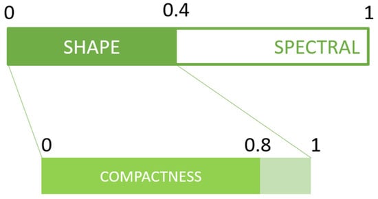
Figure 4.
Parameters used for the segmentation of bigger objects—field segmentation (scale factor = 700).

Figure 5.
In the images above, we see a comparison of the image before segmentation to detect large objects (a) and after segmentation (b).
After the identification of the fields and their distinction into cultivated and uncultivated fields, the rest of the not yet classified image is segmented again using a scale factor of 50 to identify small objects, such as the roofs of buildings. Shape factor and compactness have been modified to better adapt to the context in which the next classification will be performed, assuming the values of 0.3 and 0.5, respectively, recapped in Figure 6, while the bands and weights used remain unchanged, the result of the segmentation is shown in Figure 7.
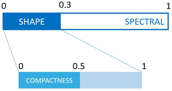
Figure 6.
Parameters used for the classification of smaller objects—urban segmentation (scale factor = 50).
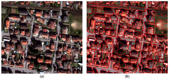
Figure 7.
The image shows a comparison between a portion of an image before (a) and after (b) segmentation for the identification of objects in the urban context.
For both segmentations performed, no detailed studies were carried out on the degree of accuracy achieved in a rigorous way. We limited ourselves to a visual check, estimating the best parameters capable of returning an identification that fits with the dimensions and edges of the perceptible elements for a human observer. We considered this step negligible because the objective of this work now is the creation of a logical scheme that, by combining the membership functions applied to the different features, leads to a correct classification and distinction of cultivated and uncultivated fields. To further increase the quality of the classification, more rigorous quality controls could be applied to the segmentation obtained [18,19] and consequently calibrate the various factors that influence it to maximize the quality of the segmentation.
2.3. Classification
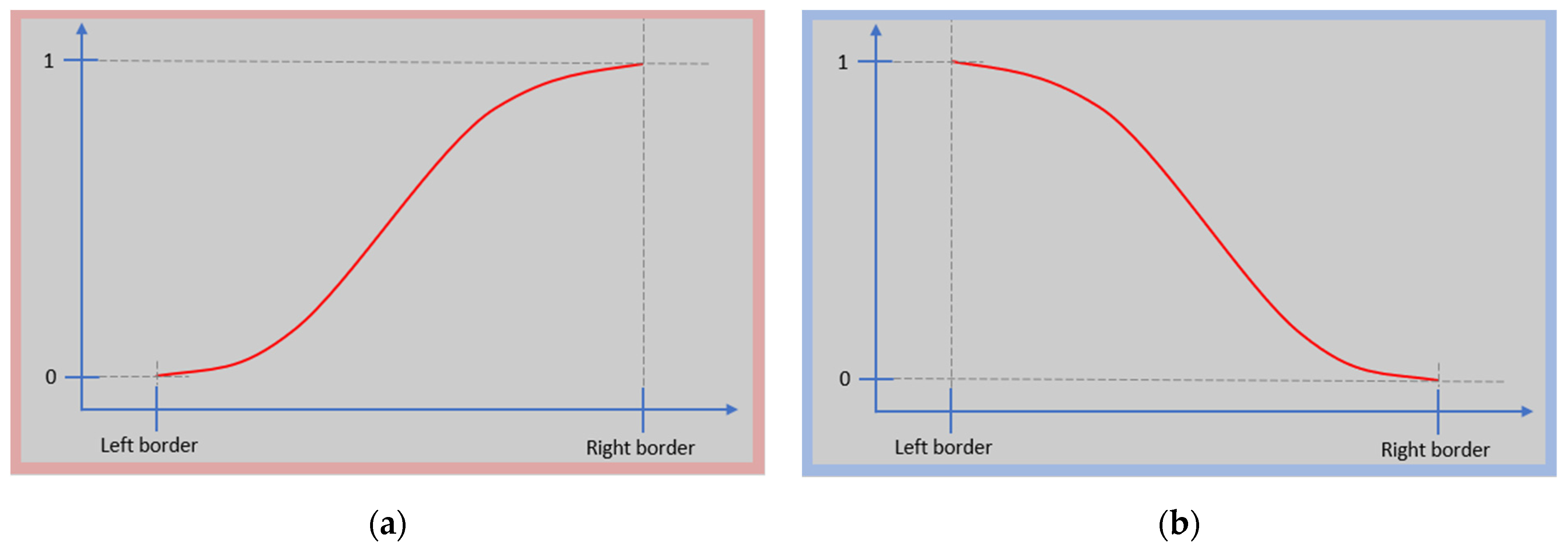
The determination of belonging to one class rather than another occurs through an accurate description of the class using a logical combination of the different features that allow distinguishing the various elements within the image. The algorithm provides two distinct classifications; the first, designed to identify objects that cover a large area, involves only the class of fields, which, once identified, are divided into the subclasses cultivated fields and non-cultivated fields, and addresses the problem of identifying these elements without them being confused with large industrial building extensions. A second classification is needed to identify the detailed elements, i.e., water and vegetation, accurately enough to leave as the only remaining elements only objects that belong to the impermeable class, i.e., roads and buildings. The fundamental block that, together with others, constitutes the description of a class is the membership function; the various classes involved are described through a logical combination of the individual membership functions, as already mentioned. In our case, only increasing, which we will call function A from now on, or decreasing function B functions are used; the two functions used can be seen in Figure 8. In this way, it is possible to smooth a threshold in a range of values between 0 and 1, which describes, if we want, in percentage, whether for that specific feature an object should belong or not to a class. If, however, a certain feature has a value less than the left border value or greater than the right border value, based on the membership function used, we will obtain a value of 1, completely belonging to that class, or 0, not belonging to that class.
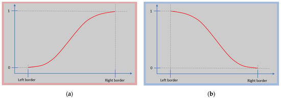
Figure 8.
Membership functions are used to assign fuzzified values to the different features used to describe the classes; in red is the increasing function (a) and in blue is the decreasing function (b).
The logical scheme, therefore, has the task of combining the results obtained from the individual membership functions to determine the percentage of membership or not for a certain class; the scheme clearly varies from class to class. For each class, the logical scheme is reported in the respective sub-chapters; for the classes involved, an accurate description was necessary only for the water and fields class, while for the vegetation class, the classification is quite straightforward using the NDVI index. These schemes were created following the logical process that a human being probably uses in recognizing those elements in the image, not only the color but also the geometric aspects.
2.3.1. Field Class
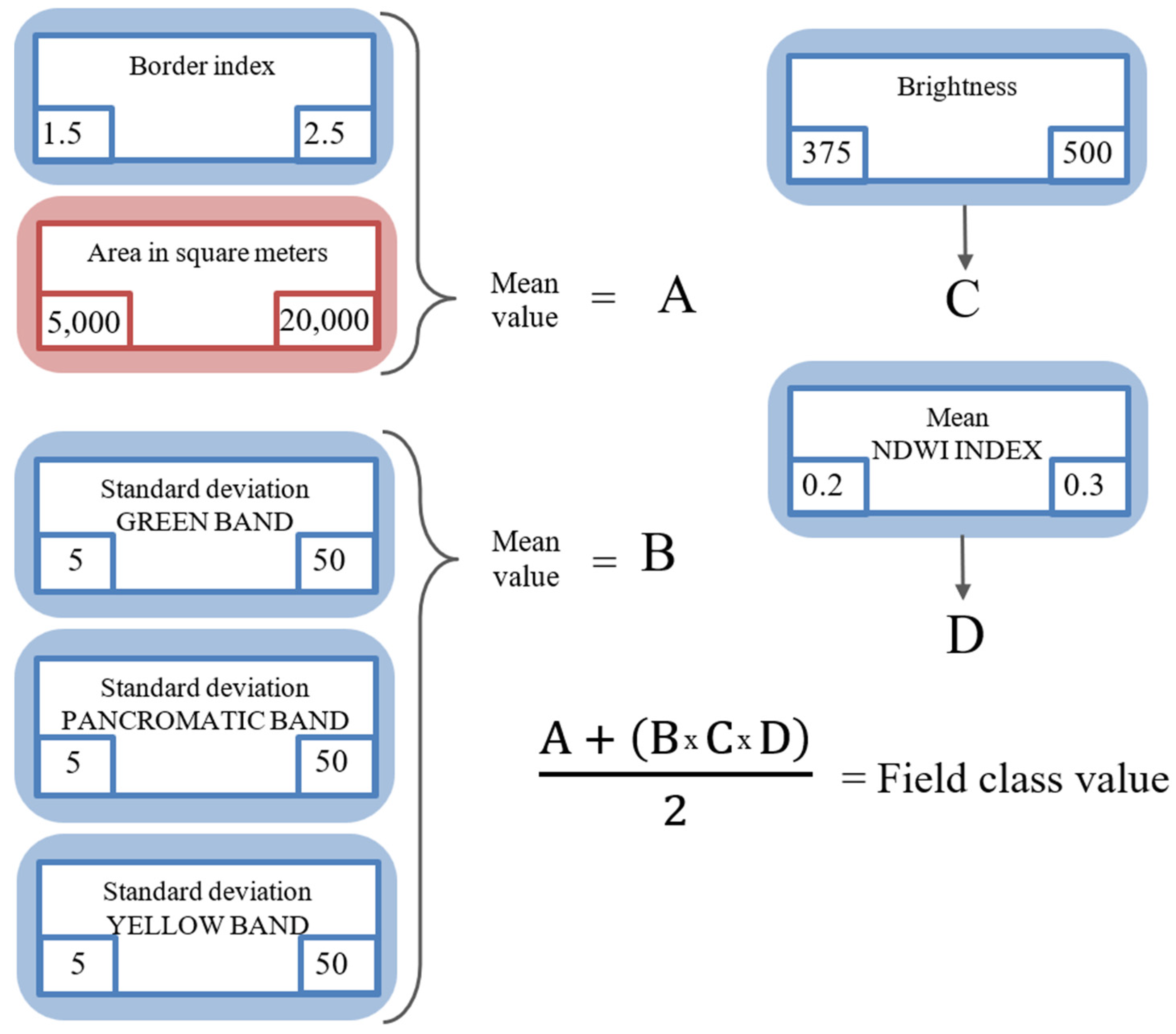
The identification of the fields occurs through the combination of the membership functions applied to the various features that characterize these objects, as indicated in the logical diagram below in Figure 9. Carrying out a specific segmentation allows us to use the geometric characteristics linked to the extension of the objects and their regular conformation through the border index. Within the eCognitionTM software, the index border is defined as the Border Index feature that describes how jagged an image object is; the more jagged it is, the higher the edge index. The smallest rectangle enclosing the image object is created, and the edge index is calculated as the ratio of the length of the object’s edge to the smallest enclosing rectangle. Typically, they tend to be regular objects, and therefore, values close to 1 well describe the regularity of the edges typical of the worked fields in the Po Valley. The geometric component A is calculated as the average between the returned value of the membership function A applied to the feature area, with respective values for the right and left border of 20,000 square meters and 5000 square meters, and the returned value of the membership function B applied to the index border, with respective values for the right and left border of 2.5 and 1.5. To evaluate the radiometric homogeneity of objects, which in the final expression we indicate with the letter B, we apply the membership function B to the internal standard deviation of the object in the green, panchromatic, and yellow bands, and we calculate the average value. Portions of urban territory identified in the segmentation phase are likely to fail to meet this homogeneity requirement because they contain many different elements, such as buildings, roads, vehicles, trees, and more. Therefore, for these elements, the parameter B will be a very small value, if not even 0. For urban portions, this requirement is very effective, while for industrial buildings, it is necessary to introduce, as an additional constraint, the C parameter of the expression, which takes into account the brightness of the objects, calculated as the sum of the visible bands (red, green, yellow, and blue).

Figure 9.
Logical scheme with which the membership functions applied to the various features involved in the identification of fields are combined, with increasing and decreasing membership functions highlighted in red and blue, respectively.
The membership function B is therefore applied in the range 375–500 of the brightness values, allowing us to filter the industrial warehouses that typically respect both the geometric and radiometric homogeneity requirements, respectively, due to their extension and the roofs typically left free. The last parameter to be inserted, called D, is obtained by directly applying function B to the average value of the NDWI index calculated on the object. This is to exclude a priori the bodies of water, which otherwise, despite having good homogeneity characteristics, may be mistakenly classified as fields. If, for us human observers, the distinction between the two types of objects is immediate and unequivocal, the addition of this fourth parameter also makes the distinction between large bodies of water and fields almost unequivocal for the software. The multiplication of the parameters B, C, and D is the most important part of the identification, in which it is fundamentally assumed that if an object is very bright, it cannot be a field regardless of whether it is homogeneous or not, and similarly, if the NDWI values are very high, the membership function goes to a value equal to or close to 0 and consequently cancels the product. If, however, the luminosity is contained within a reasonable range and the possibility that it is water is excluded, through low values of the NDWI index, we would obtain from this multiplication a weighted value based on radiometric homogeneity, a condition finally combined with the geometric requirements.
2.3.2. Cultivated and Uncultivated Fields
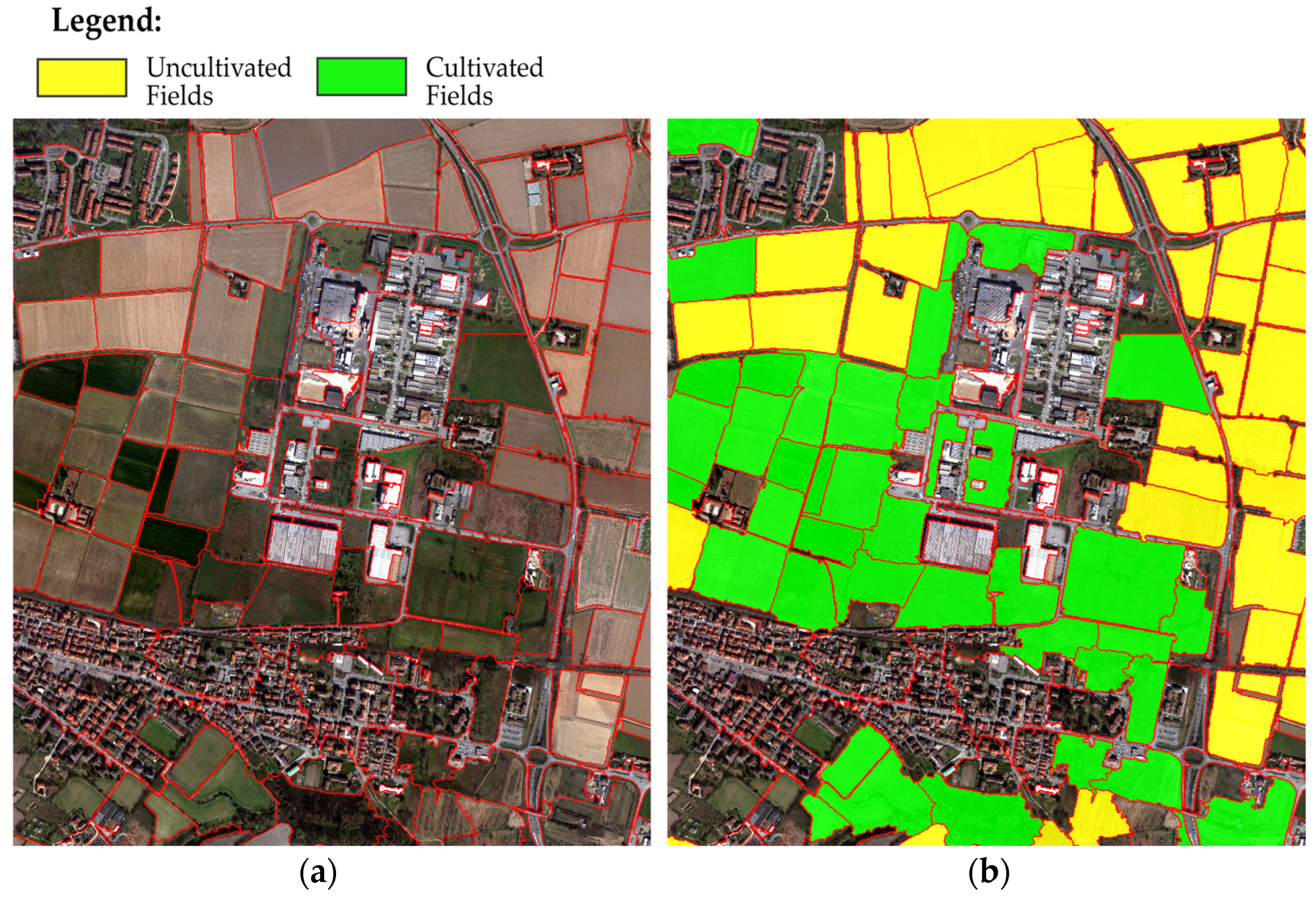
With the scheme illustrated previously, almost all fields are effectively identified by the software, regardless of the value of the NDVI index within the objects and, therefore, whether they are cultivated or not. The distinction between these two conditions is rather simple and is made by integrating at this point a threshold on the value of the NDVI index, where it is assumed that for objects classified as fields, NDVI values higher than 0.15 determine that the field is cultivated; otherwise, for lower values, the field will be considered not cultivated. The result is shown below in Figure 10.
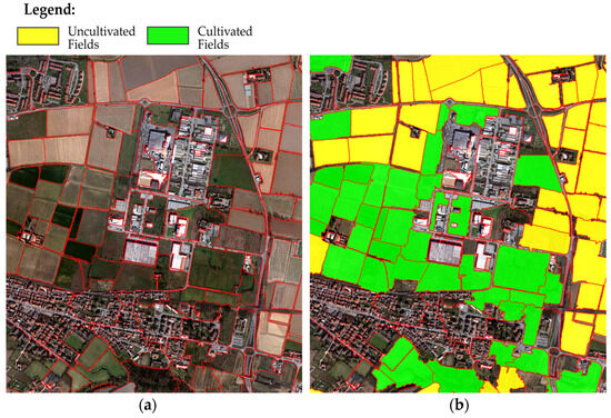
Figure 10.
The image shows the area before (a) and after (b) the classification of the fields and their further distinction into cultivated and uncultivated.
2.3.3. Water Class
The identification of water in the scene is primarily achieved using the NDVI and NDWI indices. Objects with sufficiently high NDWI index values are initially considered potential water objects. However, since shadows cast by buildings can often be erroneously included, further refinement is needed. This involves leveraging the presence of various background objects typically found in shadows, such as cars, roads, and other buildings. To address this issue, the D factor is introduced, which is derived from the standard deviation values of different bands. This factor considers the phenomenon that objects classified as water, due to their homogeneity, tend to exhibit lower standard deviation values if they are sufficiently deep. The objects that fulfill all these criteria are allocated to the water class. Any remaining objects, if they do not qualify as vegetation, are then assigned to the non-permeable soil class. The logical diagram presented below in Figure 11 was developed in a prior study that addressed the challenge of distinguishing between water and shadows in an urban environment [2]. For a more comprehensive explanation, readers are encouraged to refer to the aforementioned article.
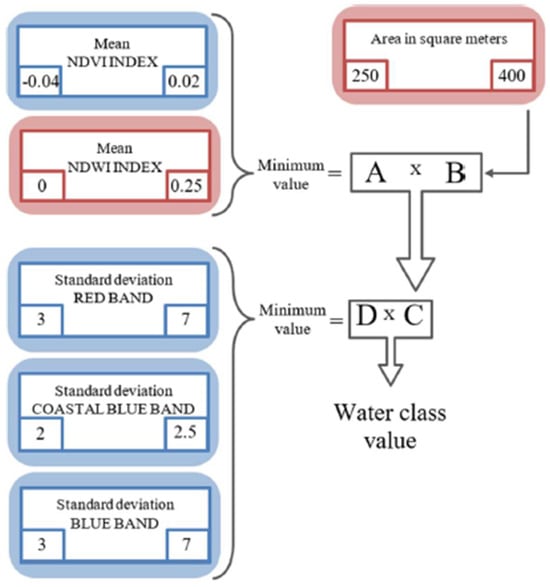
Figure 11.
Logical scheme with which the membership functions applied to the various features involved in the identification of water are combined; functions A and B are highlighted in red and blue, respectively.
2.3.4. Vegetation Class
For the identification of areas in which there is the presence of vegetation, even in urban areas, an excellent tool, which in this specific case has proven to be extremely effective, is the NDVI index. After segmenting the image, objects for which the NDVI index values are sufficiently high are classified as vegetation. In detail, the membership function A was applied to the index in the range 0.1–0.2; substantially, a threshold equal to 0.15 was applied to determine whether an object is vegetation or not. We preferred to use a membership function because, in this way, we obtain a value between 0 and 1 based on the NDVI index. Doing so, if an object had a membership value of 0.51 for the vegetation class and a membership value for the slightly higher water class, it would be attributed to the water class rather than vegetation, as would happen in the case of a threshold. It is necessary to take into consideration that the classification of the image depends greatly on the period of the year in which it is acquired; in our case, the month of March, not all plants have fully developed foliage. For this reason, it is possible to correctly classify the impervious soil part of the roads that have trees on the sides, which would otherwise also be classified as vegetation.
2.3.5. Impermeable Class
Since the main purpose of my work concerns the classification of images for the creation of soil permeability maps, no distinction is made between the elements present in the urban area. Both buildings, building roofs, and asphalt roads are not permeable surfaces, and therefore, no distinction is made between the two. Having classified all the other classes present in the image, the objects that have not been assigned to any class at this point are, therefore, assigned to the impermeable soil class. The distinction between the various elements that make up this class is in itself a separate problem and, as such, deserves to be explored in depth with specific research that goes beyond the objective we have set ourselves for this work.
2.4. Refinement Process
The refinement of the classification obtained is carried out after both segmentations and classifications, both for the identification of fields and for the identification of detail elements. For the water class, first all the objects classified in this class that are not in contact with other objects belonging to the same class are eliminated; this is necessary to remove a small portion of objects that represent shadow areas from the classification obtained. It is not always necessary, but given that the size of a stream or a small lake tends to allow for more objects inside them to be classified as water, this step constitutes a further check that the possible incorrectly classified shadows proceed in the next steps. Subsequently, the merge object fusion function is applied; this function allows you to merge adjacent objects if certain parameters are respected. For example, if an object classified as water is in contact with other objects in which a value belonging to the water class is found to be greater than 0.2, the two objects are merged precisely because water tends to be continuous, both in the form of a river and a lake. From this result, we then pass through another function present within the software, called Pixel-Based Object Resizing, where, essentially always exploiting the fact that bodies of water are continuous in nature, the objects belonging to the water class are grown in adjacent pixels if they have an NDWI index value greater than 0.3. By doing so, as we have seen in a previously published study [2], it is possible to define the edges of a watercourse very precisely.
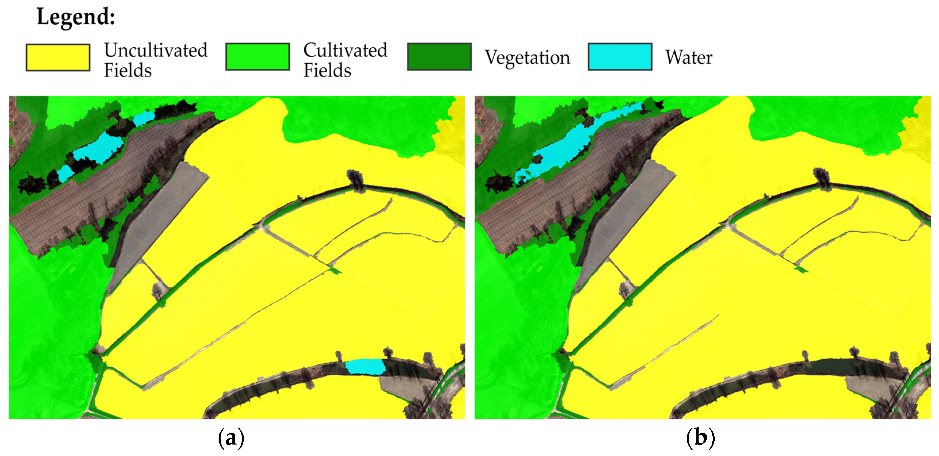
At each cycle, the water objects enlarge in the neighboring pixels, and this operation is repeated until there are no more variations in the objects present in the image, as in the example area shown in Figure 12. The next phase consists of refining the uncultivated fields that have been identified. In this case, only the merge object fusion function is used because, following the detailed segmentation adjacent to the objects classified as uncultivated fields, long-limbed objects are created; therefore, if these new objects respect certain values, they are aggregated with the existing objects. It is not necessary to carry out this operation on cultivated fields because the edges tend to be in contact with objects that will already be classified as vegetation. Even compared to what happens for the water class, in this case, the effect of the refinement is more modest; it helps us to better define the edges for uncultivated fields, as seen in the example below in Figure 13.

Figure 12.
Comparison between the water classified in the scene before (a) and after refinement (b).
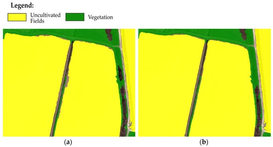
Figure 13.
Comparison between an example field before (a) and after refinement (b).
A small portion of unclassified objects is added in the right field, and in the left field, a slight addition takes place, which regularizes the border. In some cases, between one field and another, there may be a canal used for irrigation, and it is probably for this reason that these parts are not classified, as in this case, they may contain small portions with vegetation rather than exposing their surface, which is made of concrete and is, therefore, not classified. In the image shown, this effect extends, probably due to the pansharpening effect, which for small objects tends to spread the color slightly into the neighboring pixels, and therefore, a band lateral to the field is not classified. However, we believe the quality objective has been achieved given the extensive classified area, the results obtained both on the fields and on the water present in the scene, and the limits that prevent the algorithm from further improving the classification.
3. Results
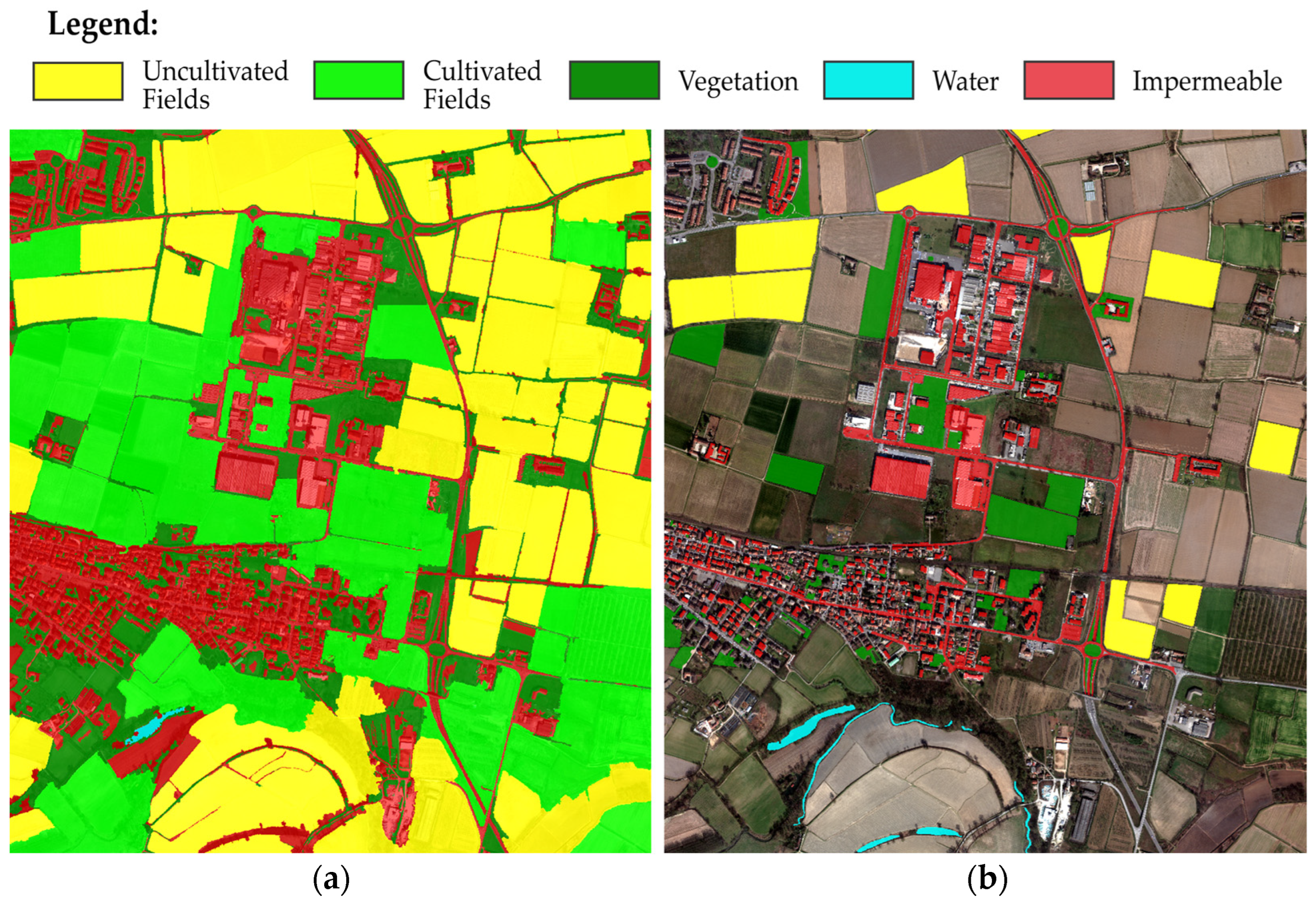
Figure 14, shown below, displays the results of the classification, with impermeable objects shown in red, uncultivated fields in yellow, cultivated fields in light green, water in blue, and vegetation in green. For comparison purposes, a shapefile was specifically created within ArcGIS Pro, containing several objects belonging to the impermeable fields, water, and vegetation classes. These objects were manually identified by a user, who observed the image and determined the edges of the objects as accurately as possible. During the comparison phase, cultivated fields were merged into the vegetation class, and individual pixels belonging to the ground truth were compared with the corresponding pixels in the classified image. From this comparison, a confusion matrix was derived, summarizing the achieved accuracy. In the lower part of the image, what immediately catches the eye is the presence in the ground truth of a small stream of a lake mainly used for agricultural purposes, which the developed classification algorithm is not able to identify. This is mainly due to the small size of the objects in that area and the presence of trees, which largely cover the path of the stream. Although the trees are bare enough to allow the operator to see the stream and identify it, radiometrically, they reflect enough light in the near-infrared wavelength to mask it from the algorithm’s eyes. This condition was not present in the area used for the development of the logical scheme of the water class since it was an urban environment; therefore, we are not surprised that this error was made, while the distinction between water and shadows, the objective for which it was developed, is carried out very well.

Figure 14.
In the images above, we see a comparison of the result obtained from the classification of the study area (a) and the ground truth created manually for validation in the same area (b).
The result is that these objects, due to this particular interaction, as the water class has been described, are not suitable to be part of it and, at the same time, do not have high enough NDVI index values due to the thin foliage of the trees to be classified as vegetation. Unfortunately, this ultimately leads to the attribution of the impermeable soil class to objects, for which it is obvious that this should not be the case. In cases where the vegetation is sufficiently abundant, the small portions of the river are incorporated into larger objects classified as cultivated fields or into objects of the vegetation class. However, it is a less impactful scenario, given our ultimate goal of obtaining a soil permeability map from the classification result. From the comparison between the results obtained from the classification by applying the developed algorithm and the ground truth identified in the study area, a confusion matrix and an accuracy matrix were derived and reported, respectively, in Table 1 and Table 2 below.

Table 1.
Confusion matrix.

Table 2.
Accuracy matrix.
In the first table for each column, we see the corresponding class in which the same pixel was classified. As an example, of the 251,804 ground truth pixels that were cataloged as water, 60,357 pixels were classified by the software as water class, 59,486 pixels as vegetation class, and 108,647 pixels as uncultivated fields, while in the second table, the corresponding accuracies are shown. Ultimately, an overall accuracy of 95.32% and a Cohen’s kappa coefficient of 0.93 were achieved in the analyzed area.
4. Discussion
As we have seen, there are difficulties in classifying small watercourses, for which the presence of tree foliage is a significant problem, due to the acquisition period, which we remember took place in March 2021. Fortunately, for the applications we are aiming for, this defect does not have major repercussions. The problem is mainly linked to the classification of water, which, if present in small-sized elements, is difficult to identify and is mainly linked to the fact that the image resolution is not sufficient. If we consider that the “real” data used have 120 cm of resolution on the ground, we realize that those rivers are only 2/3 pixels wide, and if there are trees, the radiometric data are significantly altered, considerably complicating correct identification. Furthermore, as mentioned in the belief, this error in the failure to identify water is due to the fact that the logical scheme developed to distinguish between water and shadows in an urban context. Therefore, this result can be seen from two points of view; on the one hand, it highlights the need to improve the water class description if there is a need to at least partially identify these small elements. On the other hand, the effectiveness of what has been developed is confirmed; in the area studied, there are no shadows, neither in the urban area nor outside it, incorrectly classified as water, which is a non-negligible result.
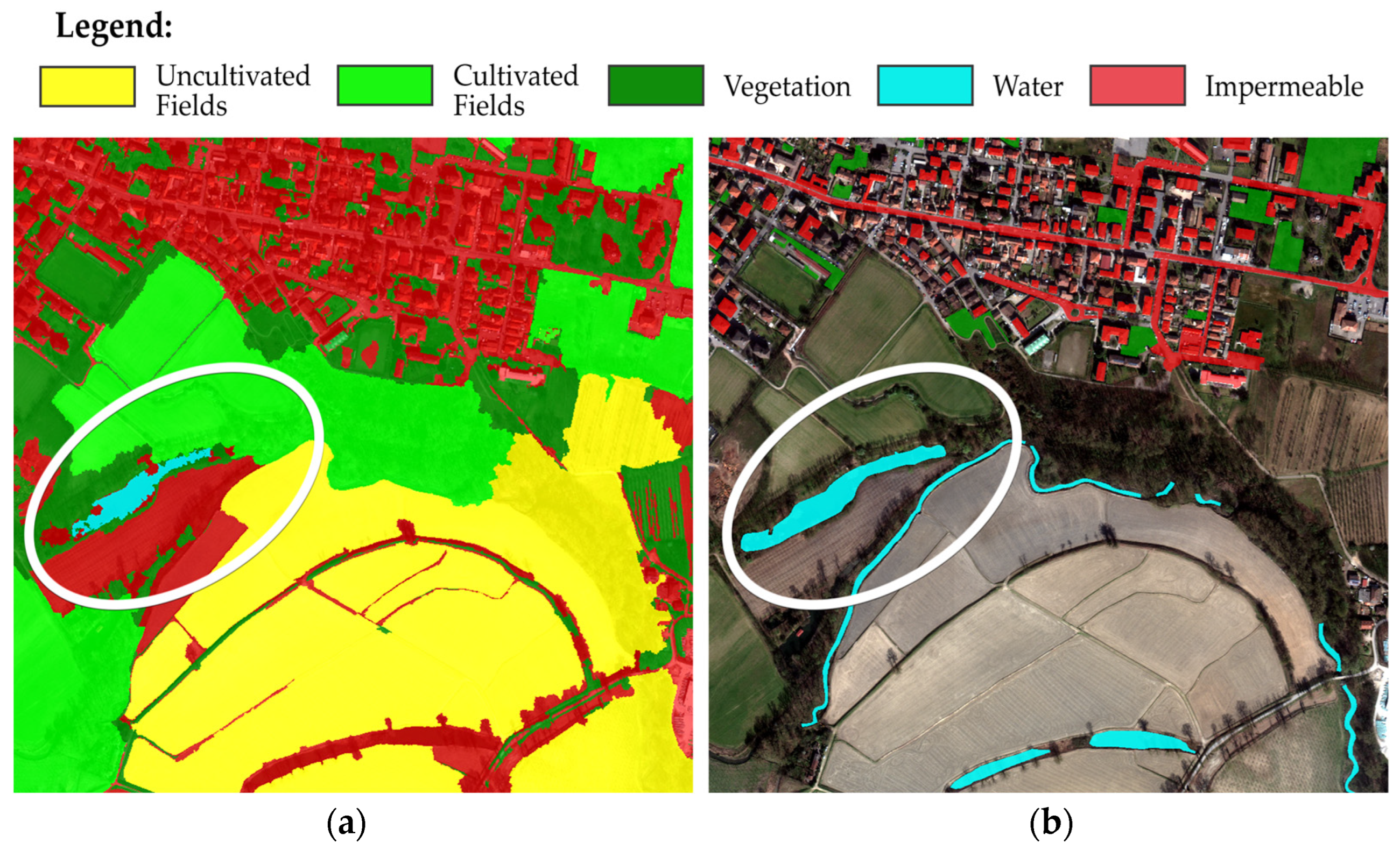
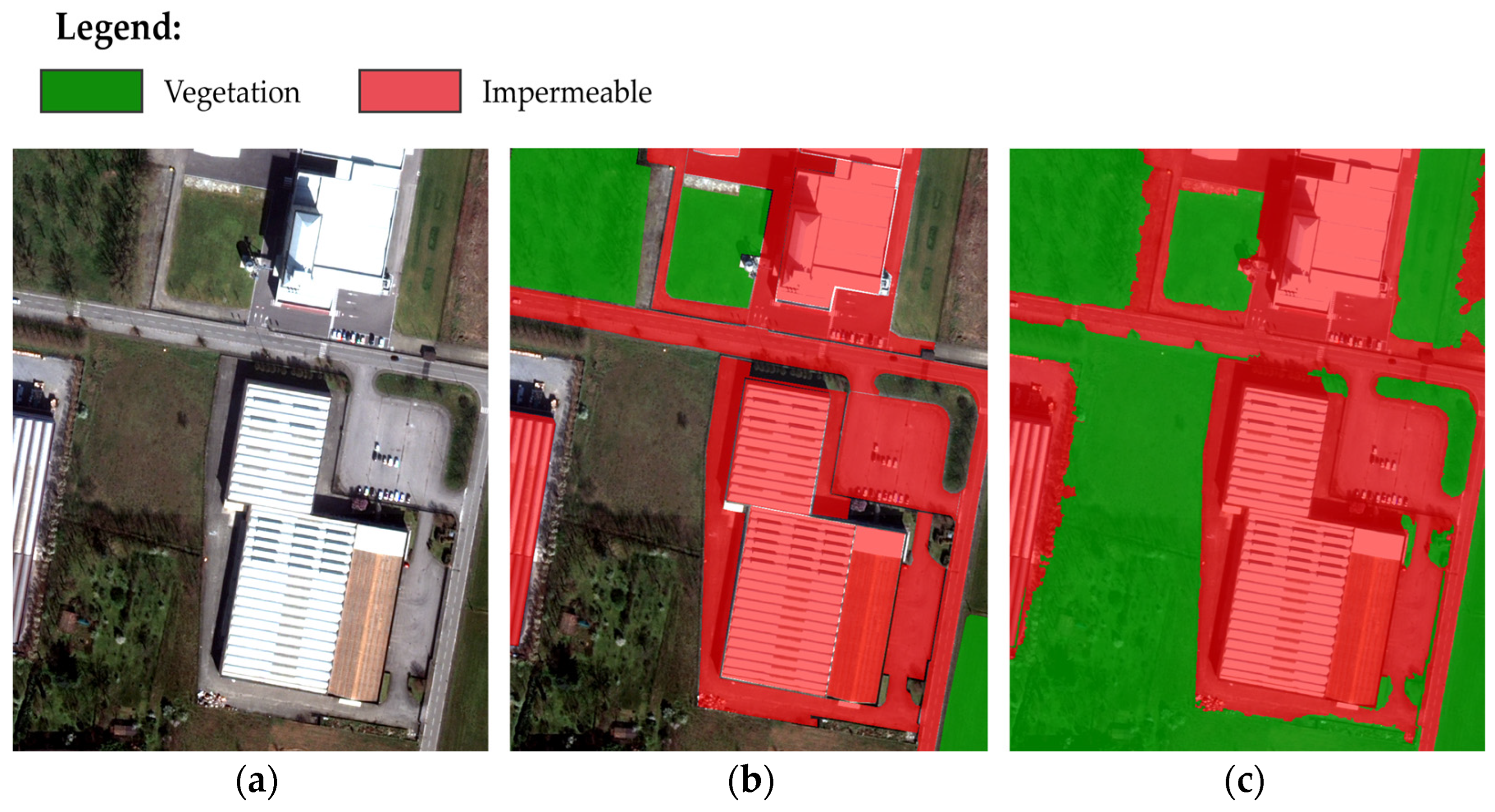
More impactful is the incorrect classification of the field adjacent to the small watercourse, which involves the attribution of the impermeable class to a fairly large surface, highlighted above in Figure 15. In the validation, that particular field was not taken into consideration; however, we can make some considerations regarding the accuracy obtained, in particular underscoring that the extension of the fields plays a fundamental role both in the classification and in the final validation. In the specific case over the entire area, the greatest classification error occurred precisely in this case, and even if the erroneously classified area is considerable (39,167.46 m2), compared with the overall extension of the uncultivated fields present in the classified (2,072,011.59 m2) image, it is reduced to a very low error percentage of 1.89%. Therefore, it is not considered necessary to modify the description currently adopted for the identification of cultivated and uncultivated fields to try to fix this error, which, as demonstrated by the results, has an excellent success rate in identifying these elements. It must also be considered that there are cases in which the result obtained is very satisfactory, where the result obtained reflects almost perfectly what the operator identified in the ground truth. As shown in Figure 16, the parts of non-permeable soil and those that are permeable in the form of vegetation are almost perfectly identified; in this case, the software also outlines the roads and edges of the square serving the shed very well. Therefore, after taking these cases into account, we can state that we are satisfied with the result obtained from the sole application of the developed algorithm, considering that errors of a gross nature, such as the incorrect classification of the fields shown in Figure 16, can always be easily fixed by the user in a review phase of the result obtained. Another aspect that can certainly be improved is the image creation process through pansharpening; currently, in the ArcGISTM software, it is possible to perform pansharpening by applying the Gram–Schmidt orthogonalization only on four bands (R, G, B, Nir).

Figure 15.
Comparison between the area affected by the classification error shown in the classified image (a) and in the ground truth (b).

Figure 16.
Comparison Example of an area in which the adopted method gave excellent results: (a) portion of the raw image; (b) ground truth identified; (c) classification result.
Based on the sensor that acquired the image, the software proposes a different weight for each band to adjust its contribution to creating a low-resolution panchromatic. These weights depend on various factors and are available by default for the four bands listed above. For the other four bands at our disposal—Coastal Blue, Yellow, Red Edge, and Nir 2—the same weights have been adopted, knowing that this necessarily introduces an error in the final result when these four bands are shown at high resolution. This necessarily presupposes a recalibration of the parameters involved when the pansharpening technique is changed or the weights with which to combine the various multispectral bands to form the low-resolution panchromatic are optimized. The technique used at this stage of development clearly presupposes the presence of an operator ready to recalibrate the parameters involved in the description of the classes as the analyzed image changes. The logical process that links and combines the membership functions between them can be considered valid, and for the water class, it has been proven valid, where there is only the need to improve the identification of small watercourses in the case in which they are partially covered by vegetation. Making the parameter calibration process automatic would constitute a notable step forward towards the application of this methodology for the segmentation phase using segmentation procedures already present in the literature [18]. While for the optimization of the values to be attributed to the right and left limits of the membership functions, for the average values of the bands, it could be interesting to use auto-threshold algorithms or, alternatively, to statistically analyze the values adopted in the classification of the image in this work and contextualize them in the overall image analyzed. Subsequently, test on a new image to see whether, by fixing the parameters a priori and applying the same correlations to the radiometric aspects of the new image, the results obtained are good or not. From what emerged from the application of the water logic scheme, it seems that this operation is not necessary if only the region studied is changed. It would certainly be interesting to test the defined parameters on a more current image acquired from the same satellite, and only through a rigorous comparison would we have confirmation or not of the real degree of dependence on the calibration of the parameters involved in the proposed method. It must also be taken into consideration that the classification obtained is absolutely independent of the ground truth, and this represents an advantage compared to machine and deep learning techniques. Creating ground truth is very time-consuming, whether you create it manually or extract it using different methods [20], even more so if part of this information must be used as examples to train this kind of algorithm. Also, in this case, the algorithms must be trained on the basis of the radiometric information of the image, and therefore, the process must be repeated if the sensor that acquires the image changes.
5. Conclusions
In conclusion, the work carried out allowed us to evaluate the effectiveness of the description of the water class previously developed in another work on a different area of the city of Pavia, discovering limitations due to the presence of vegetation but confirming its effectiveness in distinguishing between water and shadows. Furthermore, the logical scheme describing the field class has been improved, producing excellent results without misclassifying any industrial building, which had been our main problem in previous tests. The distinction between cultivated and uncultivated fields was added later, given the simplicity with which it is possible to identify them, even if it does not constitute essential information for the creation of soil permeability maps. We are satisfied with the results obtained, considering that we are still working to improve the classification result and to make it less dependent on the region studied, reducing its dependence on the recalibration of the parameters involved from time to time. I can imagine an improvement in the classification, in particular, given the critical issues with small watercourses, to further improve the potential of the methodology adopted in identifying land use. Similarly, although not fundamental for the creation of soil permeability maps, the distinction of impervious elements could be evaluated and addressed as a separate problem to distinguish in detail between the portions of soil representing buildings or roads and further enhance the ability to classify land use. Ultimately, the proposed methodology allowed us to achieve an overall accuracy equal to 95.32%, a result that I consider very satisfactory if we consider that this result takes into consideration the small quantity of water present in the scene, which, with a success rate of 23.97%, significantly lowers the overall accuracy achieved on the classification of the entire area. Future developments can certainly concern an improvement in the phase of the creation of the high-definition multispectral image through pansharpening. In my opinion, this constitutes the most critical step because we know for sure that it introduces the Coastal Blue, Yellow, Red Edge, and Nir2 bands, an error because the weights adopted for the creation of the low-resolution panchromatic, even if they are an approximation, are not correct. Ideally, I would like to finish developing an algorithm in Matlab to create the image in a single step through the pansharpening process that adopts the Gram–Schmidt orthogonalization algorithm to have more control over the individual factors that influence the result and have a final product in which the distortion of the original data of the multispectral bands in the final high-resolution image is minimal. Further progress can be obtained by inserting another step in the refinement phase, as highlighted in this work, and trying to extract, if possible, from objects classified as cultivated fields or vegetation any small and partially hidden waterways to improve further the quality of the result obtained. In the last few years, experiments have been carried out in various test areas. The one shown in this work is only the latest, and the results achieved suggest that the methodology adopted can give good results in very different situations, such as urban, rural, and mixed contexts, and therefore, it is suitable for carrying out the classification of the entire area of the municipality of Pavia.
Author Contributions
Conceptualization, V.C.; methodology, D.P.; supervision, V.C.; writing—original draft preparation, D.P. All authors have read and agreed to the published version of the manuscript.
Funding
This research received no external funding.
Data Availability Statement
The datasets presented in this article are not readily available because the data are part of an ongoing study. Requests to access the datasets should be directed to the Geomatics laboratory of the University of Pavia.
Acknowledgments
The development of my research as part of my PhD studies was partly financially supported by the PRIN project named GIANO (Geo-Risks Assessment and Mitigation for the Protection of Cultural Heritage).
Conflicts of Interest
The authors declare no conflicts of interest.
References
- Zheng, Z.; Zhong, Y.; Wang, J.; Ma, A.; Zhang, L. Building Damage Assessment for Rapid Disaster Response with a Deep Object-Based Semantic Change Detection Framework: From Natural Disasters to Man-Made Disasters. Remote Sens. Environ. 2021, 265, 112636. [Google Scholar] [CrossRef]
- Perregrini, D.; Casella, V. Classification of Water in an Urban Environment by Applying OBIA and Fuzzy Logic to Very High-Resolution Satellite Imagery. In Geomatics for Environmental Monitoring: From Data to Services; Borgogno Mondino, E., Zamperlin, P., Eds.; Springer Nature Switzerland: Cham, Switzerland, 2024; pp. 285–301. [Google Scholar]
- Cantrell, S.J.; Christopherson, J.B.; Anderson, C.; Stensaas, G.L.; Ramaseri Chandra, S.N.; Kim, M.; Park, S. Open-File System Characterization Report on the WorldView-3 Imager System Characterization of Earth Observation Sensors; U.S. Geological Survey: Sioux Falls, SD, USA, 2021. [Google Scholar]
- Maurer, T. How to Pan-Sharpen Images Using the Gram-Schmidt Pan-Sharpen Method—A Recipe. Int. Arch. Photogramm. Remote Sens. Spat. Inf. Sci. 2013, XL-1/W1, 239–244. [Google Scholar] [CrossRef]
- Björck, Å. Numerics of Gram-Schmidt Orthogonalization. Linear Algebra Appl. 1994, 197–198, 297–316. [Google Scholar] [CrossRef]
- Laben, C.A.; Brower, B.V. Process for Enhancing the Spatial Resolution of Multispectral Imagery Using Pan-Sharpening. U.S. Patent 6,011,875, 4 January 2000. Volume 11. [Google Scholar]
- Yilmaz, V.; Serifoglu Yilmaz, C.; Güngör, O.; Shan, J. A Genetic Algorithm Solution to the Gram-Schmidt Image Fusion. Int. J. Remote Sens. 2020, 41, 1458–1485. [Google Scholar] [CrossRef]
- Baatz, M.; Schape, A. Multiresolution Segmentation—An Optimization Approach for High Quality Multi-Scale Image Segmentation Angewandte Geographische Informationsverarbeitung XII. Proc. Angew. Geogr. Inf. Verarb. XII 2000, 5, 12–23. [Google Scholar]
- Pettorelli, N.; Ryan, S.; Mueller, T.; Bunnefeld, N.; Jedrzejewska, B.; Lima, M.; Kausrud, K. The Normalized Difference Vegetation Index (NDVI): Unforeseen Successes in Animal Ecology. Clim. Res. 2011, 46, 15–27. [Google Scholar] [CrossRef]
- McFEETERS, S.K. The Use of the Normalized Difference Water Index (NDWI) in the Delineation of Open Water Features. Int. J. Remote Sens. 1996, 17, 1425–1432. [Google Scholar] [CrossRef]
- Wan, J.; Yong, B. Automatic Extraction of Surface Water Based on Lightweight Convolutional Neural Network. Ecotoxicol. Environ. Saf. 2023, 256, 114843. [Google Scholar] [CrossRef] [PubMed]
- Li, L.; Su, H.; Du, Q.; Wu, T. A Novel Surface Water Index Using Local Background Information for Long Term and Large-Scale Landsat Images. ISPRS J. Photogramm. Remote Sens. 2021, 172, 59–78. [Google Scholar] [CrossRef]
- Shao, Y.; Taff, G.N.; Walsh, S.J. Shadow Detection and Building-Height Estimation Using IKONOS Data. Int. J. Remote Sens. 2011, 32, 6929–6944. [Google Scholar] [CrossRef]
- Shi, L.; Zhao, Y. feng Urban Feature Shadow Extraction Based on High-Resolution Satellite Remote Sensing Images. Alex. Eng. J. 2023, 77, 443–460. [Google Scholar] [CrossRef]
- Gao, B.C. NDWI—A Normalized Difference Water Index for Remote Sensing of Vegetation Liquid Water from Space. Remote Sens. Environ. 1996, 58, 257–266. [Google Scholar] [CrossRef]
- Huang, S.; Tang, L.; Hupy, J.P.; Wang, Y.; Shao, G. A Commentary Review on the Use of Normalized Difference Vegetation Index (NDVI) in the Era of Popular Remote Sensing. J. For. Res. 2021, 32, 1–6. [Google Scholar] [CrossRef]
- Roznik, M.; Boyd, M.; Porth, L. Improving Crop Yield Estimation by Applying Higher Resolution Satellite NDVI Imagery and High-Resolution Cropland Masks. Remote Sens. Appl. 2022, 25, 100693. [Google Scholar] [CrossRef]
- Chen, Y.; Chen, Q.; Jing, C. Multi-Resolution Segmentation Parameters Optimization and Evaluation for VHR Remote Sensing Image Based on Mean NSQI and Discrepancy Measure. J. Spat. Sci. 2021, 66, 253–278. [Google Scholar] [CrossRef]
- Zhao, M.; Meng, Q.; Zhang, L.; Hu, D.; Zhang, Y.; Allam, M. A Fast and Effective Method for Unsupervised Segmentation Evaluation of Remote Sensing Images. Remote Sens. 2020, 12, 3005. [Google Scholar] [CrossRef]
- Shetty, S.; Gupta, P.K.; Belgiu, M.; Srivastav, S.K. Assessing the Effect of Training Sampling Design on the Performance of Machine Learning Classifiers for Land Cover Mapping Using Multi-Temporal Remote Sensing Data and Google Earth Engine. Remote Sens. 2021, 13, 1433. [Google Scholar] [CrossRef]
Disclaimer/Publisher’s Note: The statements, opinions and data contained in all publications are solely those of the individual author(s) and contributor(s) and not of MDPI and/or the editor(s). MDPI and/or the editor(s) disclaim responsibility for any injury to people or property resulting from any ideas, methods, instructions or products referred to in the content. |
© 2024 by the authors. Licensee MDPI, Basel, Switzerland. This article is an open access article distributed under the terms and conditions of the Creative Commons Attribution (CC BY) license (https://creativecommons.org/licenses/by/4.0/).


