Abstract
Due to a unique imaging mechanism, Synthetic Aperture Radar (SAR) images typically exhibit degradation phenomena. To enhance image quality and support real-time on-board processing capabilities, we propose a lightweight deep generative network framework, namely, the Lightweight Super-Resolution Generative Adversarial Network (LSRGAN). This method introduces Depthwise Separable Convolution (DSConv) in residual blocks to compress the original Generative Adversarial Network (GAN) and uses the SeLU activation function to construct a lightweight residual module (LRM) suitable for SAR image characteristics. Furthermore, we combine the LRM with an optimized Coordinated Attention (CA) module, enhancing the lightweight network’s capability to learn feature representations. Experimental results on spaceborne SAR images demonstrate that compared to other deep generative networks focused on SAR image super-resolution reconstruction, LSRGAN achieves compression ratios of in model storage requirements and in computational resource demands. In this work, we significantly reduce the model complexity, improve the quality of spaceborne SAR images, and validate the effectiveness of the SAR image super-resolution algorithm as well as the feasibility of real-time on-board processing technology.
1. Introduction
Synthetic Aperture Radar (SAR) serves as a sophisticated active microwave remote sensing imaging radar system, distinguished by its capability for all-weather, round-the-clock terrestrial observations. Spontaneously, SAR has become established as a pivotal technological approach within the modern remote sensing domain. The operating principle of SAR systems involves transmitting and receiving radar waves and utilizing moving platforms (such as aircraft or satellites) to synthesize a larger virtual antenna to achieve high-resolution (HR) images of the Earth’s surface. The technology not only possesses the ability to penetrate the surface, offering insights through cloud layers and vegetation cover, but also demonstrates significant resistance to interference, ensuring stable operation under diverse environmental conditions. SAR technology plays an indispensable role across various fields, including topographic mapping, environmental monitoring, natural disaster assessment, agricultural yield estimation, and national security, underscoring its unique value and crucial impact [1]. For instance, SAR technology provides essential data support in the environmental monitoring realm by tracking forest logging, desertification processes, and changes in sea ice. Additionally, in the aftermath of natural disasters, SAR technology is instrumental in assessing the damage and impact of earthquakes, floods, and landslides, thereby guiding disaster response and recovery efforts. Within the domain of national security, SAR technology is utilized for terrain reconnaissance, target tracking, and the detection of concealed objectives, showcasing its key role in military surveillance and strategic deployment.
Due to the unique imaging mechanism of SAR, the quality of the actual SAR images obtained is associated with severe degradation phenomena such as speckle, ambiguity, and sidelobes. The higher the quality and the richer the information content of SAR images are, the greater the possibility and accuracy of target recognition in application interpretation [2]. Therefore, obtaining HR SAR images has become one of the key objectives in the development of SAR technology. Image super-resolution (SR) is a technological means to improve the quality of SAR images. In the process of obtaining SAR images, there are typically two categories of factors that lead to a reduction in the resolution of the images obtained, thereby affecting their quality. One category is the inherent resolution limitations of the SAR system itself, which prevent the images from achieving the desired effects, with improvements or updates to equipment not only being costly and time-consuming but also likely to be constrained by technological development. The other category includes the unavoidable influences of various interference factors during the image acquisition process, such as non-ideal movements of the platform, atmospheric disturbances, less-than-ideal imaging conditions and system noise. Factors can cause image blurring, defocusing, and geometric deformation, further reducing resolution and image quality. Given the difficulty and cost of physically improving the resolution of SAR images, designing algorithms to enhance the resolution of SAR images has become a cost-effective and feasible solution [3]. Consequently, image reconstruction algorithms aimed at increasing resolution have attracted increasing attention from researchers, and enhancing image resolution has become one of the most active research areas in the field of image processing.
SAR image SR algorithms are primarily divided into two major categories: traditional analytical methods and methods based on deep learning. Traditional analytical approaches achieve significant results by establishing physical models of the degradation process and employing optimization algorithms to solve ill-posed inverse problems. Freeman et al. [4] introduced a sample-based SR analytical technique, and algorithms based on sparse representation via compressive sensing theory have been proven effective tools for addressing SAR image SR issues [5,6,7]. Karimi et al. [8] combined adaptive compressive sensing with sparse priors to propose a new SAR image SR method based on conjugate gradient least squares. However, due to the highly nonlinear models upon which traditional analytical methods are based, they have a high computational complexity and struggle to process HR, wide-swath SAR images, resulting in low processing efficiency. Furthermore, the necessity for manual adjustment of model parameters for different scenes and systems limits the adaptability of these algorithms.
Given these challenges, deep learning methodologies, which have achieved revolutionary advances in various disciplines, offer an innovative solution for SR in SAR images. Driven by large-scale sample data, deep learning approaches can achieve complex nonlinear fittings, bypassing the tedious process of mathematical modeling and parameter selection and significantly enhancing algorithm performance and efficiency by shifting the time cost from application to training phase. However, most existing deep learning methods are developed within the optical image domain and may not adapt well to the unique characteristics of SAR images when directly applied, thereby affecting the quality improvement of the images [9,10,11]. Moreover, deep learning models typically have complex structures and numerous parameters, requiring high-performance hardware platforms, posing challenges for the deployment of spaceborne radar systems in orbit and on portable devices. Therefore, investigating how to maintain network performance while reducing model computational complexity, i.e., the network lightweight techniques of deep learning, has become key to the timeliness and adaptability of spaceborne SAR image SR processing.
The primary focus of this work is the introduction of a lightweight SAR image SR network, named Lightweight Super-Resolution Generative Adversarial Network (LSRGAN). The network effectively reduces the complexity of the original Generative Adversarial Network (GAN) model by using Depthwise Separable Convolution (DSConv) techniques. Additionally, we have incorporated an improved attention mechanism and introduced a novel activation function. Ultimately, LSRGAN not only achieves a significant reduction in the volume of model parameters (by ) but also accelerates the convergence speed of model training while essentially maintaining the model’s original performance. The innovative design not only enhances the SR effects of SAR images but also provides new technical support for the implementation of real-time, in-orbit processing techniques.
The structure of this paper is organized as follows: Section 2 provides a comprehensive review of related work, discussing image SR methods based on deep learning and techniques for lightweight networks. Section 3 introduces the proposed network architecture and offers a detailed description of each component within the network. Section 4 presents detailed experimental results of the proposed method and conducts a comparative analysis with other GAN approaches in the current SAR domain. Section 5 concludes the paper.
2. Related Works
2.1. SAR Image Super-Resolution
In the realm of deep learning, methods for image SR were initially applied and rapidly developed within the optical domain. Dong et al. [9] were the first to introduce convolutional neural networks (CNNs) to the field of image SR, proposing the Super-Resolution Convolutional Neural Network (SRCNN). The work marked a pivotal transition in image SR technology from traditional algorithms to deep learning approaches. Dong et al. [10] further incorporated deconvolution layers into the SRCNN framework to process low-resolution (LR) images, achieving a training speed increase of over 40 times while ensuring reconstruction quality. Enhanced Deep Super-Resolution (EDSR) and Multi-scale Deep Super-Resolution (DSR) systems proposed by Lim et al. [11] enhanced the reconstruction effects by deepening the network structure. However, as the network depth increased, the marginal effects on performance improvement gradually diminished. The emergence of GAN represents a significant milestone in deep learning. The Super-Resolution Generative Adversarial Network (SRGAN) introduced by Ledig et al. [12], which incorporated a perceptual loss function, was able to restore realistic textures from highly downsampled images and achieve impressive visual effects. Enhanced Super-Resolution Generative Adversarial (ESRGAN) proposed by Wang et al. [13] further improved network performance by comparing the relative real probabilities of SR images and HR images. Pathak et al. [14] established an Attentional Super-Resolution Generative Adversarial Network (A-SRGAN) to achieve SR of images on a large scale. The Deep Plug-and-Play Super-Resolution (DPSR) designed by Zhang et al. [15], with its plug-and-play feature, can process any blurry LR images.
SAR images differ significantly from optical images in terms of physical properties, imaging mechanisms and image morphology, which has resulted in the deep learning-based SAR image SR techniques still being in an exploratory phase. Shen et al. [16] proposed the Polarimetric SAR Image Super-Resolution (PSSR) technique, which significantly improved spatial resolution while preserving the detailed information of the image well. Duan et al. [17] introduced an improved residual network that reduces redundant computation by removing the Batch Normalization (BN) layers. Li et al. [18] proposed a Feature Reuse Dilated-Residual Convolutional Neural Network (FRDRCNN) that incorporates a perceptual loss, achieving precise semantic-level SAR image SR and, especially, showing stronger visual effects in the SR of small objects and the reconstruction of edges and contour information. To fully utilize the information in LR images, Xiao et al. [19] developed an SAR image SR algorithm based on Cross-Resolution Discrimination (CRD) using a teacher–student network concept, which not only ensures more high-frequency texture details of HR images but also accurately achieves downsampling to the original LR images. Li et al. [20] proposed a Multi-Scale Learning Based Optical Image Guidance Network (MLOG) to fully utilize the feature information of HR optical images to assist in the SR of SAR images. Wang et al. [21] applied SRGAN to SAR image SR, and experiments proved that the reconstruction effect of this deep learning algorithm is superior to traditional Bicubic methods. Zheng et al. [22] introduced a Self-Normalizing Generative Adversarial Network (SNGAN) that shows good performance in improving the resolution and object recognition capability of SAR images. However, most existing deep learning methods for image SR are developed in the optical domain, and their direct application to SAR images can affect the quality improvement. Therefore, to address the issue of suboptimal enhancement effects caused by variations in image characteristics, we have implemented modifications to the activation functions within the Lightweight Residual Modules (LRMs) and introduced an optimized Coordination Attention (CA) mechanism. This approach is designed to enhance the model’s adaptability to diverse image attributes and improve the overall processing efficacy, thereby significantly boosting the performance of image processing tasks.
2.2. Lightweight Technology
In network models for deep learning, the pursuit of high performance often comes with an increase in network depth or width, a process that inevitably introduces a large number of parameters and computational complexity. The increase not only raises the requirements for hardware platforms but also hinders the deployment of models on portable devices and platforms with limited resources. Therefore, designing lightweight neural network models that maintain high performance with fewer parameters becomes key to further addressing the issue of model real-time performance.
In recent years, the emergence of lightweight neural network models and model compression techniques has propelled the wide application of deep learning technologies in mobile and embedded devices [23], especially playing a significant role in fields such as smart homes, security and surveillance, and intelligent driving. Convolution, as the core component of network models, occupies the majority of the network parameters. Therefore, lightweight processing of convolution modules is crucial for achieving and overall lightweight network model. Early lightweight models [24,25,26,27] used DSConv and group convolutions, where DSConv [28] significantly reduces the network’s parameter count and computational complexity, showing a great effect in model compression. Further research, such as the lightweight asymmetric DSConv network proposed by Wang et al. [29] and the lightweight precision convolution based on DSConv by Jang et al. [30], demonstrated the potential of networks to enhance feature extraction capability while maintaining efficient computation. Additionally, group convolutions [31], by decoupling standard convolutions, improved the sparsity between filters, thereby achieving a reduction in model parameters and a regularization effect. With the introduction of attention mechanisms, the performance of lightweight network models has been further improved. The new lightweight network based on multi-attention mechanisms (LACN) established by Fan et al. [32] effectively extracted detailed features and suppressed noise, while the VLESR method proposed by Gao et al. [33] better propagated and fused local features, thereby enhancing image quality. Despite the limitations in depth and channel count that may lead to decreased performance and limited feature expression capability compared to general CNN models, the design of dynamic convolutions [34] seeks a balance between network performance and computational load without increasing network width and depth by merging multiple convolution kernels to enhance the model’s feature expression capability.
In the field of image SR, efforts to reduce the computational complexity and save storage space have led to the exploration of lightweight SR networks [35,36,37]. Guo et al. [38] proposed a Lightweight Multi-Dimension Feature Fusion Network (LMDFFN) for optical image SR, which maintains high reconstruction quality with fewer parameters and reduced computational complexity. Shi et al. [39] introduced a dual-prior network for optical remote sensing image SR, showing better reconstruction effects under multiple degradation factors but with a significant increase in the number of parameters as the iteration number increases, necessitating a balance between algorithm performance and computational efficiency. Shen et al. [40] presented a Reparameterizable Multibranch Bottleneck Network (RMBM-MC) for lightweight optical image SR, achieving better SR effects with very low parameter counts and efficient deployment of edge computing devices. Xu et al. [41] proposed a Structure Preservation Super-Resolution Reconstruction Network (SP-SRNet) algorithm for satellite SAR images, utilizing a lightweight deep CNN to extract image gradient map features, providing more structural information for the SR network, and designing an objective function comprised of pixel loss and gradient loss for network optimization. Zhang et al. [42] implemented SAR image SR using the lightweight network SqueezeNet [24], achieving considerable reconstruction effects with reduced computational complexity.
With the rapid development of lightweight technologies, preliminary successes have been achieved in fields such as optics. In contrast, the research on lightweight technologies in the radar domain is still in its infancy. Therefore, this study designs and implements a novel plug-and-play LRM aimed at providing new technical support for real-time on-board processing technologies for spacebore SAR.
3. Method
In this section, we present the overall architecture of the proposed network and elaborate on the optimization strategies and methods for several key components within the network structure. Furthermore, we also provide detailed descriptions of the loss function’s composition and its calculation methods. The research focuses on SR tasks for SAR images and aims to enhance the network’s capability in feature extraction and utilization through advancements in the network structure, while maintaining a relatively low model complexity. The following sections detail the design philosophy of each part and their roles in improving network performance.
3.1. Network Structure
The overall network architecture of the LSRGAN method primarily comprises two core components: the Generator Network (G) and the Discriminator Network (D). Through a dynamic “game process”, both networks conduct an alternating optimization strategy, allowing for gradual improvements in their respective performances throughout the optimization process. The interaction and balance between G and D are critical in driving the continuous self-optimization and performance enhancement of LSRGAN during the iterative process. Importantly, the dynamic balancing mechanism ensures that the network effectively addresses various challenges during iterations, culminating in the HR generation of target SAR images.
As shown in Figure 1, the core design of G comprises the LRM and CA modules. The LRM is a low-requirement and low-computational network component developed based on the concept of DSConv [25,26]. The component efficiently extracts both shallow and deep features from LR SAR images and features strong transferability, facilitating plug-and-play application for model compression of various network models. The use of BN layers to standardize data distribution across layers is a conventional practice in CNNs. The method utilizes batch-wise mean and variance for feature normalization during the training phase and employs the estimated mean and variance from the training set during the testing phase. However, significant statistical differences between the training and test sets may impede the generalization capability of network models, especially in image SR tasks where the use of BN layers can also deteriorate the contrast information of images. Without BN layers, training becomes challenging, leading to the risk of the network getting stuck in local optima and failing to converge. Therefore, in our G, redundant BN layers have been tactically removed to ensure rapid convergence and improved output quality, as elaborated in Section 3.2 of the paper. Additionally, to further enhance the network performance, the CA module is introduced. The module employs two one-dimensional feature encoding processes along different directions, generating feature maps capable of directional and positional perception. These feature maps complementarily enhance the representation of targets of interest, with a detailed description provided in Section 3.3.
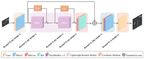
Figure 1.
Schematic diagram of the Generator Network structure with corresponding kernel size, number of feature maps, and stride.
In G, the relationship between the LR and HR SAR image is expressed as follows:
in this framework, and represent the and SAR images, respectively, where w and h signify the width and height of and W and H signify the width and height of , assuming an SAR image comprises C color channels. is a feedforward neural network parametric by , where encapsulates the network weights and biases across L layers. These parameters are refined through the minimization of the loss function . Furthermore, and represent the training data pairs of the nth set of LR and HR SAR images, .
As shown in Figure 2, D adopts a CNN as its foundational architecture, integrating DSConv within its intermediate layers to reduce the model’s parameter and computational complexity. Moreover, to mitigate the issue of gradient vanishing that may arise during the training phase, the network incorporates Leaky Rectified Linear Unit (LeakyReLU) activation functions. When an input image is processed through a convolutional layer with a stride of 2, the dimension of the output image is correspondingly reduced. Following this, the number of feature maps supplied to the next convolutional layer is increased to twice that of the previous layer. The methodology not only reduces the spatial dimensions of the image but also significantly enhances the feature extraction capability of the network.
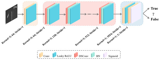
Figure 2.
Schematic diagram of the Discriminator Network structure with corresponding kernel size, number of feature maps, and stride.
Following the definitions provided by Goodfellow et al. [43], we construct D, which is alternately optimized with G to address the max–min problem encountered in the adversarial process. The objective function of LSRGAN is expressed as follows:
D and G constitute two independent network architectures. In Equation (2), the inner maximization part defines the objective function of D and essentially involves learning and optimizing while keeping fixed aiming to maximize the differentiation between HR SAR images and SR SAR images. Another aspect of the outer minimization part of Equation (2) defines the objective function of G, aimed at optimizing under the condition that remains unchanged, to generate SR SAR images that closely approximate HR SAR images. Therefore, through the cyclic iteration and mutual adverse optimization strategies of and during the training process, the networks promote each other’s improvement, ultimately training a G network capable of deceiving D, thereby solving the image SR problem.
In traditional methods, the loss function of G typically employs the Mean Squared Error (MSE), a method that calculates the loss at the pixel level. However, the approach can lead to blurred images, thereby losing high-frequency detail information. In contrast, the loss calculation at the feature level takes into account the structural information of images, such as edges and shapes. Constraining the SR and HR SAR images at the feature level effectively prevents the blurring of reconstructed images, thereby enhancing their visual perceptual quality. Ledig et al. [12] proposed a perceptual loss function that consists of two components: content loss and adversarial loss. Content loss is used to constrain consistency between SR and HR SAR images at the feature level, while the adversarial loss is a common form in GANs. This is discussed in detail in Section 3.4.
3.2. Residual Module Improvements
In recent years, CNNs have made significant progress across various fields. As research into these networks progresses, scholars have discovered that the capability of the network to extract features is determined by the number of layers in the network. However, during the process of increasing the number of network layers, a phenomenon known as network degradation occurs, where the loss function value during training progressively declines and tends toward saturation, but when the depth of the network is further increased, the numerical value of the loss function paradoxically begins to rise, resulting in difficulties in network convergence and diminished performance. In 2015, the Residual Network (ResNet) achieved groundbreaking results in the ImageNet competition, successfully addressing the issue of network degradation. ResNet incorporates residual modules with skip connections that pass input directly to the subsequent layer, enabling deeper network structures and reducing the risk of overfitting.
In the deep neural field, the overarching research trend is to construct deeper and more complex network architectures to enhance performance [44]. However, alongside the pursuit of task completion accuracy, the parameter count and computational complexity of network models are key considerations in the design process. In real-world applications, such as autonomous vehicles, mobile device utilization, and satellite technology, there is often an aim to achieve the highest possible accuracy within the constraints of limited computational resources [45]. Consequently, designing lightweight networks becomes a challenge, especially in the context of spaceborne radar’s need for real-time processing of SAR images. The objective is to ensure that the model is compact while maintaining excellent network performance. We adopt the SRGAN as the foundational framework, selecting its G as the core structure. The feature extraction portion of G utilizes the classic architecture of ResNet. To reduce the network’s parameter count and computational complexity, we introduce improvements to the residual block. The core strategy leverages the conceptual framework of the MobileNet series by incorporating DSConv into the network architecture with specific optimizations, thereby constructing a plug-and-play LRM. The goal is to reduce the network model’s reliance on computational resources and to enhance its convergence speed.
3.2.1. Depthwise Separable Convolution
The concept of DSConv was first introduced in [28] and has become a hallmark in the design philosophy of the MobileNet series of lightweight network models. As shown in Figure 3, the novelty of the structure lies in decomposing the standard convolution operation into two distinct processes: depthwise convolution and pointwise convolution. Specifically, depthwise convolution applies a filter to each input channel individually for feature extraction, followed by pointwise convolution that fuses these features on a per-pixel basis, thereby decomposing the convolution operation. Compared to standard convolutions that apply filters to all input channels simultaneously for feature extraction and fusion, the decomposition strategy of DSConv significantly reduces the model’s parameter count and computational resource consumption while largely maintaining network performance. This offers an efficient structural optimization strategy for lightweight network design. Such optimization is especially valuable and widely applicable for deploying network models on resource-constrained devices, particularly in scenarios requiring real-time processing and low-power operation.
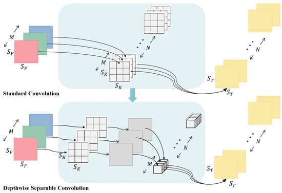
Figure 3.
Convolution structure, it includes both standard convolution and depthwise separable convolution. In the illustration, the left and right sides represent the input and output images respectively. The input image displays different channels in red, green, and blue, while the output image is shown in yellow. The central part of the diagram elaborately depicts the core transition process from standard convolution to depthwise separable convolution.
A feature map F of size is input into a standard convolution layer, which outputs a feature map T of size . In the formulation, and represent the width and height of feature maps F and T, respectively, while M and N denote the input and output channel counts of the network model. The standard convolution layer is parameterized using a convolution kernel K with dimensions (). The computation process for the output feature map is defined as follows:
then, the calculation of the parameter count for standard convolution is given by the following:
The introduction of DSConv alters the traditional interaction pattern between the number of output channels and the convolution kernels. In DSConv, each input channel corresponds to an independent convolution. Therefore, the output mapping computation process for the DSConv layer is defined as follows:
where is the depthwise convolution kernel of and the mth convolution kernel in is applied on the mth channel to generate the mth channel on the convoluted output feature map ; the calculation of the parameter count for depthwise convolution is as follows:
to generate new features, it is necessary to utilize pointwise convolutions in conjunction, enabling the output of linear combinations of features. Consequently, the computational cost of DSConv is calculated as follows:
that is, the computation of DSConv is the sum of depthwise convolution and pointwise convolution computation.
From Equations (4) and (7), we have
here, the number of channels is typically large, rendering the effect of negligible. Consequently, compared to standard convolution, the computational cost of DSConv can be by approximately times. In this study, DSConv is applied not only to enhance residual blocks but also to compress the parameter count of D.
3.2.2. SeLU Activation Function
The activation function in networks serves as a functional transformation between the input and output layers, aiming to enhance the model’s expressive power by introducing non-linearity. The widely used Rectified Linear Unit (ReLU) activation function is favored for its low computational complexity and effectiveness in mitigating issues like overfitting, gradient vanishing, and gradient explosion. However, ReLU can cause a gradient vanishing when the input values are negative, preventing model parameter updates. Consequently, researchers have proposed several variants of ReLU, such as Parametric Rectified Linear Unit (PReLU), LeakyReLU, and Scaled Exponential Linear Unit (SeLU), etc., which can circumvent the gradient vanishing issue. In the task of SR of optical images, networks typically use ReLU or PReLU as the activation function. However, analysis of the spatial dimension reveals that the scattering information in SAR images exhibits characteristics of point-like discreteness, and the observational dimension dependencies indicate that SAR images possess discontinuities, such as flickering. These characteristics are markedly different in optical images.
Klambauer et al. [46] introduce the SeLU activation function, which incorporates a self-normalizing mechanism. The mechanism automatically adjusts the mean and variance of the network’s outputs to be close to 1 during the training process, effectively mitigating the issue of network adaptability caused by the excessive disparity in scattering information within SAR images. When the input to the SeLU is negative, its output exhibits exponential growth. Conversely, for positive inputs, the output approximates linear growth. At near zero input values, the output of the SeLU approximately follows a Gaussian distribution, which contributes to enhancing the generalization capability of the network. The mathematical expression for the is as follows:
here,
3.2.3. Lightweight Residual Module
The DSConv technique decomposes the standard convolutional kernels into a layer of depthwise convolution and a layer of pointwise convolution, fundamentally changing the parameter computation in convolutional operations from traditional multiplicative accumulation to additive accumulation between two separate terms. The technology significantly reduces complexity of the model, not only decreasing the storage space required on hardware platforms but also effectively enhancing computational efficiency. It holds substantial practical application value in optimizing deep learning models and their efficient computation.
Inspired by the DSConv technology, we have designed a novel LRM that reduces network complexity by utilizing DSConv without BN layers, making the module more suitable for SR tasks. Furthermore, by replacing all activation functions within the module with SeLU, which specifically introduces a self-normalizing mechanism, the mechanism can automatically adjust the mean and variance of the network outputs during the training process. The enhanced network configuration, when combined with residual connections, not only facilitates efficient information transmission within deep networks but also improves the network’s adaptability to SAR images, while mitigating problems related to gradient explosion and vanishing during network training. As shown in Figure 4, the inclusion of a CA module at the end of the LRM (see the study in Section 3.3) provides the module with computational efficiency and storage convenience while maintaining or even enhancing model performance. This renders it appropriate for implementation on devices with constrained resources, striking an effective balance between processing speed and output quality.
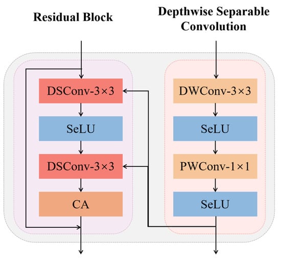
Figure 4.
Lightweight Residual Module; DWConv, and PWConv are depthwise convolution and pointwise convolution, respectively.
3.3. Coordinate Attention
In the realm of deep learning, attention mechanisms emulate human visual and cognitive systems, enabling CNNs to focus on parts of the input data that are closely related to the task at hand. The essence of the mechanism lies in the efficient utilization of limited information resources by emphasizing key feature information while suppressing less relevant details, thereby enhancing the network model’s feature extraction and recognition capabilities. Specifically, by incorporating attention mechanisms, CNNs are capable of automatically identifying and prioritizing crucial information within the input data, which significantly boosts the network’s performance and generalization ability. In recent years, a vast array of attention mechanisms has been proposed and extensively integrated into network architectures for executing a variety of tasks. For the design of lightweight networks, researchers generally prefer the Squeeze-and-Excitation (SE) [47] module. However, SE primarily focuses on interactions between channels and often neglects processing key spatial location information crucial for understanding object structures in visual tasks. Although attention mechanisms such as Bottlenet Attention Module (BAM) [48] and Convolutional Block Attention Module (CBAM) [49] attempt to capture positional information by applying convolution operations after reducing channel dimensions, the approach only enables the extraction of local relationships and is insufficient for capturing long-range dependencies, which becomes a limitation when dealing with complex visual tasks.
Hou et al. [50] introduced a Coordinated Attention (CA) mechanism tailored for lightweight networks, aimed at decomposing channel attention into two unidirectional feature encoding processes that aggregate features along distinct spatial directions. The methodology not only captures long-range dependencies along a particular spatial direction but also preserves precise positional information in another direction. Consequently, the feature maps extracted via convolution are effectively encoded into a pair of attention maps with directional and positional awareness, thus enhancing the network’s ability to accurately retain critical feature information. Considering the potential negative impacts of BN layers on super-resolution tasks, we have optimized the CA module as depicted in Figure 5.
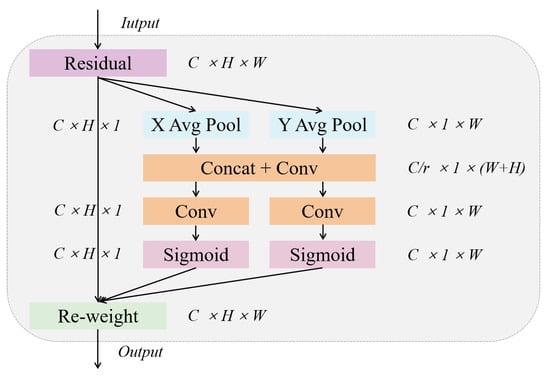
Figure 5.
Coordinate Attention module.
The CA module applies global average pooling along the width and height dimensions of the input feature map, thereby obtaining feature maps for these two dimensions. The process facilitates the capture of attention along the height and width of the image and encodes precise positional information. Specifically, for the input feature map , horizontal and vertical features are encoded by applying pooling operations with kernel sizes of and , respectively. Consequently, the representation of the dimension feature along the width and height directions can be described as follows:
where is the output that is associated with the channel.
The process outlined above generates a pair of feature maps with directional awareness capabilities, significantly enhancing the network’s accuracy in locating objects of interest. Subsequently, these two feature maps, oriented in different directions, are concatenated to form an aggregated feature map. The map is then transformed by a convolution function , which uses a kernel, reducing its dimensionality to of the original dimension. In the context of SE, the parameter r denotes the reduction ratio, which governs the extent to which the dimensionality of the module is reduced, as depicted in the following expression:
in the equation provided, denotes a concatenation operation along spatial dimensions, and represents a nonlinear activation function. Here, is a feature map of dimensions, which encodes spatial information in both horizontal and vertical directions. The feature map is decomposed along the spatial dimensions into two independent tensors, and . Subsequently, each tensor is processed by utilizing convolution transformation functions and with convolution kernels. The specific processing steps are outlined as follows:
where is the sigmoid function. Ultimately, the output of the CA module is as follows:
3.4. Loss Function
The loss function of the LSRGAN method still consists of two parts: the weighted sum of content loss and adversarial loss , specifically as follows:
here, the mathematical expressions for the and are as follows:
where denotes the feature mapping of the jth convolution layer before the ith pooling layer in the network, is the probability that the reconstructed image is a natural HR image. To obtain a better gradient, minimize .
4. Experiments
4.1. Software and Hardware Configuration
High-performance computing hardware can significantly reduce the training time required for neural network models and enhance the speed of model convergence. When these hardware configurations are paired with suitable deep learning frameworks, further improvements in overall model performance may be achieved. In our study, we train the relevant network models on a computer hardware system equipped with an NVIDIA GeForce RTX 3080 GPU using the dataset constructed in this paper. For each mini-batch, we crop 16 random HR SAR sub-images of distinct training images, and the loop is executed 500 times, i.e., . To optimize the training process, we use the Adam optimizer [51], maintaining its default parameter settings (, and ). All experiments are conducted on a computer with a 64-bit Windows 11 operating system, supported by software including Pytorch 1.12.0, CUDA 11.6, and Python 3.8.
4.2. Evaluation Indicators
In this study, five significant objective metrics for image quality assessment, Peak Signal-to-Noise Ratio (PSNR), Structural Similarity Index (SSIM), Visual Information Fidelity (VIF), Equivalent Numbers of Looks (ENL), and Radiometric Resolution (RaRes), are selected to objectively evaluate the efficacy of SR algorithms for SAR images. PSNR measures the degree of distortion in processed images by calculating the differences between the original images and the processed results, mainly reflecting the maximum possible error in the signal. SSIM analyzes and compares the original and processed images from the multi-dimensional aspects of image luminance, structural information, and contrast, representing an image quality assessment method that closely aligns with human visual perception. VIF quantifies the degree image improvement by computing mutual information between the original and the processed images. ENL assesses the relative strength of speckle within SAR images. RaRes evaluates the capability of SAR images to distinguish between objects based on the radiometric quality of individual pixels. These metrics are widely used in fields such as SR and image compression, providing a scientific basis for quantitative analysis and comparison of the effects of different image processing algorithms.
PSNR is defined based on the MSE; for SAR images () and SAR images () of size , the is calculated as follows:
then, the mathematical expression for its is
where is defined as the maximal feasible pixel value of the , with the PSNR being expressed in dB. A greater PSNR value indicates improved quality of the reconstructed image and enhanced similarity between the two SAR images.
SSIM evaluates the similarity between the and based on three fundamental characteristics: luminance, structural information, and contrast. Essentially, it is a statistical method capable of effectively reflecting the overall structural similarity of images. The mathematical representation is as follows:
here, x and y symbolize and the , respectively. is indicative of luminance comparison, encapsulates the comparison of structural information, and represents the contrast comparison. The coefficients , , and are utilized to modulate the prominence of luminance, structural information, and contrast within the SSIM framework. When all , , and are set to 1, the following relationship holds:
where and represent the means of x and y and and represent the variances of x and y, respectively. denotes the covariance between x and y, and are constants for maintaining stability (here , and L are the dynamic ranges of the pixel values). The greater the similarity between and is, the closer the value of SSIM approaches 1 ().
The VIF index is a full-reference image quality assessment metric that is based on the statistics of natural scenes and the extraction of image information by the Human Visual (HVS). It has strong consistency with human judgments of visual quality. The fundamental concept underlying VIF is to view image quality assessment as an issue of information fidelity, quantifying and assessing the quality of an image from the perspectives of information transmission and sharing. In the VIF algorithm, and represent the information extracted from specific sub-bands of the original and processed images, respectively, by the HVS model. Assuming each wavelet sub-band is independent, the mutual information is extended across K-bands and summed to produce the objective VIF score. The specific mathematical computation is as follows:
here, K represents the number of sub-bands, while and are the mutual information measurements for the sub-band, respectively. The value of the VIF index ranges from 0 to 1. A higher VIF value indicates that the processed image retains more visual information, thereby denoting a higher image quality.
ENL is a metric used to quantify the uniformity of smooth regions. In the SAR domain, the metric is employed to assess the relative strength of speckle noise in SAR images. Specifically, ENL reflects the visual smoothness of uniform regions within the image. It can be expressed as follows:
herein, and represent the mean and variance of pixel intensity values in uniform areas, respectively. A higher ENL value indicates lower noise levels in SAR images, resulting in clearer images that facilitate more accurate visual identification and interpretation of SAR imagery.
RaRes represents the ability of SAR systems to differentiate target backscatter coefficients, serving as a measure of the SAR system’s capability to distinguish closely distributed targets. The performance of this metric directly influences the interpretation and quantitative applications of SAR images. RaRes is inversely proportional to ENL, meaning a smaller RaRes value indicates a stronger capability of the SAR system to differentiate adjacent targets, resulting in higher quality SAR images with greater application value. RaRes is defined as the ratio of the absolute deviation and mean of the reflection signal within a resolution cell relative to the mean value, which can also be expressed as follows:
in the equation above, , , and ENL represent the mean, standard deviation, and Equivalent Numbers of Looks, respectively, of the pixel intensity values in a homogeneous area.
4.3. Datasets and Materials
The MSAR-1.0 dataset [52] is an SAR image dataset targeting various scenes and categories using data from Hisea-1 and Gaofen-3 satellites. The scenes include airports, ports, coastal areas, islands, and urban areas, with images containing various types such as oil tanks, bridges, airplanes, and ships as depicted in Figure 6. The dataset consists of polarimetric SAR data, including HH, HV, VH, and VV polarization modes. The image size is , with some bridge images having dimensions of , all in JPG format with a 24-bit depth. A random selection of 1000 images are used for training, 70 images for validation, and 20 images for testing, and none of the image data overlapped.
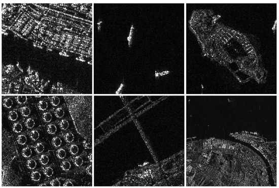
Figure 6.
Some examples of the MSAR-1.0 dataset.
The SSDD dataset [53] is the first widely used publicly available polarimetric SAR image dataset for studying ship detection based on deep learning techniques. As shown in Figure 7, it incorporates data from RadarSat-2, TerraSAR-X, and Sentinel-1 satellites. The majority of the images in the dataset contain extremely small or tiny targets, with dimensions of approximately pixels. The dataset includes SAR images with simple backgrounds and complex backgrounds. For the purpose of training, 500 images are randomly selected from the SSDD dataset, 30 images for validation, and 18 images for testing. It is important to note that none of the image data mentioned above are duplicates.
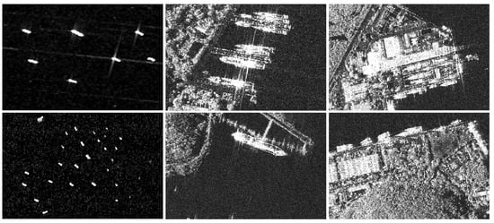
Figure 7.
Some examples of the SSDD dataset.
Merging the aforementioned data, we create a dataset for SAR image SR tasks in this paper, comprising 1500 training images, 100 validation images, and 38 testing images. To generate the corresponding LR SAR images, we applied Bicubic to downscale the HR SAR images by a factor of four. The pairs of HR and LR SAR images form the essential dataset for deploying the LSRGAN method, as depicted in Figure 8.
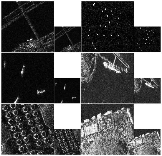
Figure 8.
Some examples of SAR image datasets in our study.
4.4. Experimental Results
We conduct a comprehensive validation of the proposed network method, including comparisons in simple scenarios (as shown in rows 1 and 2 of Figure 8) and complex scenarios (as depicted in row 3 of Figure 8) as well as across four different types. The SAR sample images used for testing include not only the test set constructed in Section 4.3 but also 20 randomly selected images from the remaining dataset of MSAR-1.0 for each category. Given that the primary aim of the study is to design a lightweight SAR image super-resolution generative adversarial network, we compare the proposed LSRGAN model with other deep generative models in the SAR image processing domain. The comparison is conducted through detailed analyses of both objective evaluation metrics and subjective visual effects. The comparison methods include Bicubic, SRGAN, and SNGAN. To ensure the fairness of the experiment, all methods are optimized with the respective best hyperparameters as described in the related papers.
4.4.1. Quantitative Results
Based on the existing GAN models in the SAR image SR domain, Table 1 provides a detailed comparison of these models in terms of the parameter count, computational complexity, time required to train for one epoch, and the time needed for a 256 × 256 SAR image. Table 2 and Table 3 offer a comprehensive comparison of the performance of various GAN for SR tasks on SAR datasets.

Table 1.
Comparison of model complexity for GAN methods in the field of SAR image SR. G and D represent the generator and discriminator networks, respectively. “M” denotes million, and “s” stands for seconds. To avoid conflicts in the representation of symbols, FLOPs are also expressed in M. The best performance is highlighted in bold.

Table 2.
Average performance of GAN methods in the field of SR of SAR images. The metric values are obtained by averaging the results from 20 SAR image tests for each type. A smaller RaRes value indicates higher image quality, while for the other metrics, the opposite is true. denotes high-resolution images, with the best performance highlighted in bold.

Table 3.
Average performance of GAN methods in the field of SR of SAR images. The metric values are obtained by averaging the results from 20 SAR image tests for each type. A smaller RaRes value indicates higher image quality, while for the other metrics, the opposite is true. denotes high-resolution images, with the best performance highlighted in bold.
As shown in Table 1, we set up three control experiments to validate the lightweight effects of the lightweight SR network. From the results, it can be observed that in terms of the number of model parameters, LSRGAN accounts for only and of the parameters compared to SRGAN and SNGAN, respectively, significantly reducing the storage requirements on hardware platforms. In terms of model computational complexity, LSRGAN reduces the computational demands by and compared to SRGAN and SNGAN, respectively, effectively lessening the computational resource requirements on hardware platforms. Additionally, LSRGAN demonstrates a clear advantage in training time, reducing the average training duration per epoch by 0.835 s compared to the other two models. In the model testing time, using the processing of a SAR image as an example, LSRGAN reduces the testing time by an average of 0.133 s compared to the other models, further showcasing the advantages of this method in processing speed.
As shown in Table 2, our network model shows some deficiencies in certain objective evaluation metrics. However, compared to SRGAN, LSRGAN achieves the best results in the VIF, indicating that our approach is more aligned with human visual characteristics, making it more suitable for the interpretation and analysis of SAR images of the human eye. The performance enhancement is particularly notable in the processing of simple scene SAR images. Although LSRGAN slightly outperforms in RaRes by 0.1648 in simple scenes compared to SNGAN, it significantly surpasses SNGAN in all other objective metrics. As shown in Table 3, a comparative analysis of four different types reveals that our method achieves the best PSNR for ships, with average improvements of 0.0283 dB and 0.0004 dB over SRGAN and SNGAN respectively, but performs slightly below the best values in processing oil tanks, bridges, and airplanes. In terms of the SSIM, our method reaches the highest scores for bridges and ships but shows weaker performance for the other two categories, with an average reduction of 0.0066. In VIF, LSRGAN achieves excellent outcomes in most scenarios, whether in diverse background complexities shown in Table 2 or various types of Table 3. In the ENL and RaRes, SRGAN consistently delivers the best results, which will guide the focus of our future research efforts. Overall, as the four types of Table 3 mostly belong to the complex scenarios of SAR images represented in Table 2, the less favorable objective metrics performance of LSRGAN in Table 3 does not contradict the findings from Table 2.
In summary, although LSRGAN does not achieve the highest objective evaluation metrics in certain scenes or types, it has demonstrated notable advantages over both SRGAN and SNGAN in terms of model complexity and the time required for image processing. It not only mitigates the performance degradation during the model lightweight process but also enhances the feasibility of implementing real-time on-board image SR technologies.
4.4.2. Qualitative Results
SAR images exhibit significant differences from the common optical images in terms of physical properties, imaging mechanisms, and morphology. Spaceborne SAR images feature a wide viewing range and rich texture details, suggesting that the HR SAR images used as label samples might suffer from issues like image smoothing, blurring, and unclear edges. The problem can contribute to lower quantitative experimental results compared to optical images. The experimental results from Figure 9, Figure 10 and Figure 11 demonstrate that although our approach has much lower model complexity than the comparative methods, it achieves comparable or even superior performance in SR experiment results across various scenes and types of SAR images.
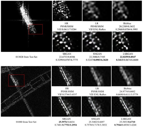
Figure 9.
Visual qualitative comparison of ships and bridges on the SAR image test set. The local magnification areas of different methods are marked with red boxes in the original image. From the images, it is evident that the sea areas occupy more than half of the space in both images, indicating that they are simple scenes. The best results are bolded.
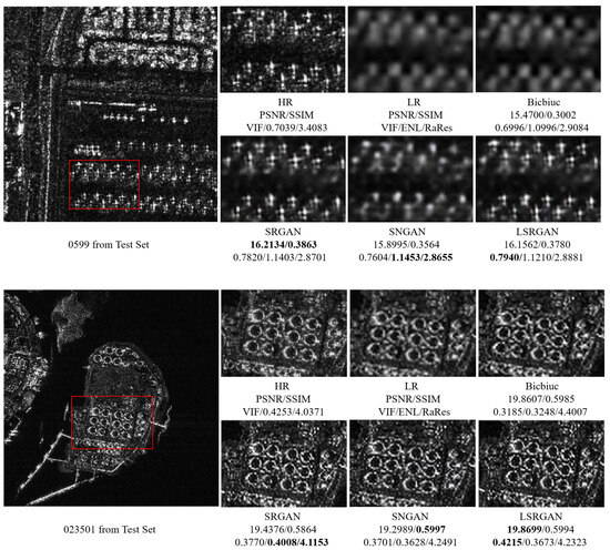
Figure 10.
Visual qualitative comparison of airplanes and oil tanks in the SAR image test set. The background of the airplane images includes airport facilities with detailed textures, categorizing it as a complex scene. The local magnification areas of different methods are marked with red boxes in the original image. For the oil tank images, both the sea areas and terrestrial features occupy about half of the image area each, with these scenes to be considered either simple scenes or complex scenes. Moreover, the values of objective evaluation metrics indicate that they fall between these two categories. The best results are bolded.
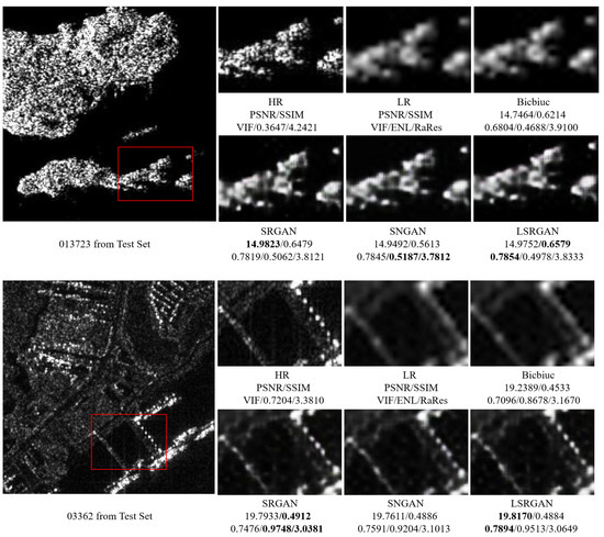
Figure 11.
Visual qualitative comparison of islands and ports on the SAR image test set. The local magnification areas of different methods are marked with red boxes in the original image. From the images, it can be seen that the sea areas occupy less than half of the image area in both pictures, indicating that they belong to simple scenes. The best results are bolded.
As shown in Figure 9, in SAR images where maritime regions occupy more than half of the image area, all models are able to accurately restore high-frequency details of ships and bridges with higher objective evaluation metrics. LSRGAN achieves the best performance on PSNR, SSIM, and VIF metrics. In contrast, for images where maritime regions occupy less than half of the image area, the objective evaluation metrics of the models are lower. As shown Figure 10, despite lower values in quantitative evaluation, key details such as the edges of airplanes and oil tanks are still clearly discernible. LSRGAN records the best results in PSNR and VIF indicating that the methodology of this work more closely aligns with human visual characteristics and the interpretation and decoding of SAR images. Additionally, as shown in Figure 11, the presence of diverse geographical features in islands and harbors resulted in complex texture details, yet LSRGAN excels in PSNR, SSIM, and VIF, providing superior subjective visual experience.
4.5. Ablation Studies
High-performance network models are typically proportional in complexity and require execution on hardware platforms with significant storage and computational power. Given the unique characteristics of SAR, spaceborne radars often face the challenge of limited resources and can only support software with low power consumption and computational capacity for real-time image processing. To explore the impact of different modules within our proposed LSRGAN, we incrementally improve upon the standard SRGAN model and conduct a comparative analysis of these enhancements. All models are trained from scratch with the same setup. As shown in Table 4, to develop a lightweight SAR image SR method, we first introduce DSConv into SRGAN. This step results in a compression of in storage requirements and of computational resource demands, leading to a slight decline in model performance (see the row labeled 2nd in Table 4). While maintaining a lower level of model complexity, the use of various modules has proven to enhance model performance (see the rows labeled 3rd and 4th in Table 4). When all modules are implemented simultaneously, the model’s storage and computational demands are reduced by and , respectively. More importantly, model performance reaches an optimal level (see the row labeled 5th in Table 4).

Table 4.
Ablation experiment results of different blocks based on SRGAN. Bold indicates best performance.
We conduct an in-depth analysis of the network performance resulting from various component combinations. As illustrated in Figure 12, at the initial stage of the training phase, there is a sharp decrease in the loss curve. However, as the number of training epochs increases, the decreasing trend gradually slows down and eventually stabilizes. Through observation of Figure 13, we find that increasing the number of training epochs and extending the training duration can assist us in achieving optimal performance for the task.
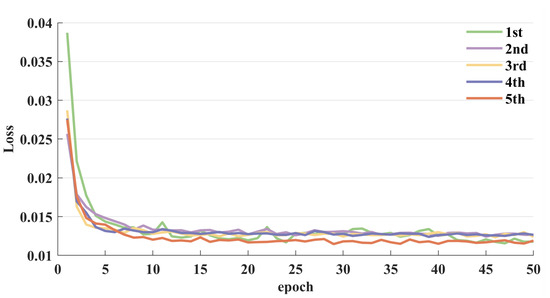
Figure 12.
Loss curves for the training of ablation experiment.
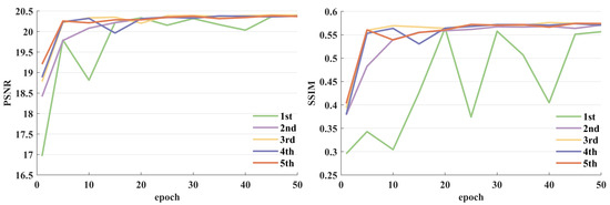
Figure 13.
PSNR and SSIM curves for training in the ablation experiment.
In Figure 13, we compare the variations in the PSNR and SSIM on the validation set throughout the model improvement process. With the application of DSConv, we observe a tendency for some convolution kernels to become null during training. The phenomenon is primarily attributed to the ReLU activation function, which causes significant information loss when processing low-dimensional inputs, in contrast to its minimal impact on high-dimensional inputs. Therefore, we initially integrate DSConv into both the generator and discriminator networks, excluding the first and last layers, to maximize model compression despite this potentially decelerating the model’s convergence speed and impacting its performance, as shown in 1st and 2nd in Figure 13.
Subsequently, alongside the introduction of the CA module, we remove all BN layers from both the CA module and DSConv. While the inclusion of the CA module enhances model performance, it also increases the model’s parameter count and complexity. The elimination of BN layers conserves computational resources and memory usage without compromising model performance, as shown in 2nd and 3rd in Figure 13. The adjustment effectively balances the model’s complexity and performance, ultimately achieving a stable and consistent performance enhancement with minimal resource expenditure. Furthermore, in the context of SR tasks, we find that models with deeper and more complex networks, incorporating multiple BN layers, are more susceptible to artifacts. To mitigate the occurrence of null convolution kernels in DSConv, we use the SeLU activation function constructs of the LRM module, aimed at improving the model’s convergence speed and generalization capability, as shown in 2nd and 4th in Figure 13.
Finally, by integrating all the improved network components, we develop the LSRGAN, achieving model stability at the fastest convergence rate, as demonstrated in 5th in Figure 13. These outcomes suggest that our approach effectively leverages the correlations between feature mappings to enhance information transfer, enabling the network to focus more on high-frequency texture details, thereby enhancing model performance while reducing model complexity.
5. Conclusions
We introduce a novel lightweight SAR image super-resolution GAN named LSRGAN to tackle the challenges of high model complexity and poor reconstruction quality found in existing deep learning-based SAR image SR methods. Specifically, we have designed a plug-and-play LRM that leverages DSConv for effective compression of the network model. During the initial training phase, standard convolutions are used to achieve dimension expansion, ensuring the rich extraction of initial features. In the inference phase, the LRM is combined with an improved CA module, achieving precise retention of key feature information while significantly reducing the number of parameters. The method not only ensures superior SR results but also reduces model complexity, thereby enhancing inference speed. Extensive experimental outcomes indicate that our network significantly improves the visual perception of SAR images, particularly in enhancing high-frequency details such as edges and textures. Compared with existing deep generative models, LSRGAN offers a superior balance in terms of SAR image reconstruction quality, model complexity, and convergence speed. Moving forward, we plan to further refine the GAN model’s scale and computational complexity to reduce the training time and hardware resource consumption required by the network.
Author Contributions
Conceptualization, J.Z. and N.J.; methodology, N.J.; software, N.J. and W.Z.; resources, J.Z. and H.W.; writing—original draft preparation, N.J.; writing—review and editing, W.Z., H.L. and Z.C. All authors have read and agreed to the published version of the manuscript.
Funding
This research was funded by National Natural Science Foundation of China (No. U22B2015).
Data Availability Statement
Publicly available datasets were analyzed in this study. The MSAR-1.0 dataset can be obtained from: https://radars.ac.cn/web/data/getData?dataType=MSAR (accessed on 26 June 2023); the SSDD dataset can be obtained from: https://pan.baidu.com/share/init?surl=l2Qs5Pd-NbMt3DUlSGxgWQ&pwd=cnh5 (accessed on 26 June 2023).
Acknowledgments
This work is partially supported by National Natural Science Foundation of China (Grant No. U22B2015), with funding and support from Shanghai Key Laboratory of Remote Sensing and Millimeter Wave Information Acquisition and Application Technology.
Conflicts of Interest
The authors declare no conflicts of interest.
References
- Xu, F.; Jin, Y.Q. Microwave vision and intelligent perception of radar imagery. J. Radars, 2024; in press. [Google Scholar]
- Yang, X.L.; Xu, D.W.; Huang, P.P.; Yang, W. Change detection of high resolution SAR images by the fusion of coherent/incoherent information. J. Radars 2015, 4, 582–590. [Google Scholar]
- Wang, Z.M.; Zhu, J.B.; Xie, M.H. Technique of SAR Image Super-Resolution, 2nd ed.; Science Press: Beijing, China, 2013; pp. 102–275. [Google Scholar]
- Freeman, W.T.; Jones, T.R.; Pasztor, E.C. Example-based super-resolution. IEEE Comput. Graph. Appl. 2002, 22, 56–65. [Google Scholar] [CrossRef]
- Dong, W.; Zhang, L.; Shi, G.; Wu, X. Image deblurring and super-resolution by adaptive sparse domain selection and adaptive regularization. IEEE Trans. Image Process. 2011, 20, 1838–1857. [Google Scholar] [CrossRef]
- He, C.; Liu, L.; Xu, L.; Liu, M.; Liao, M. Learning based compressed sensing for SAR image super-resolution. IEEE J. Sel. Top. Appl. Earth Obs. Remote Sens. 2012, 5, 1272–1281. [Google Scholar] [CrossRef]
- Kulkarni, N.; Nagesh, P.; Gowda, R.; Li, B. Understanding compressive sensing and sparse representation-based super-resolution. IEEE Trans. Circuits Syst. Video Technol. 2012, 22, 778–789. [Google Scholar] [CrossRef]
- Karimi, N.; Taban, M.R. Nonparametric blind SAR image super resolution based on combination of the compressive sensing and sparse priors. J. Vis. Commun. Image Represent. 2018, 55, 853–865. [Google Scholar] [CrossRef]
- Dong, C.; Loy, C.C.; He, K.M.; Tang, X.O. Image super-resolution using deep convolutional networks. IEEE Trans. Pattern Anal. Mach. Intell. 2016, 38, 295–307. [Google Scholar] [CrossRef]
- Dong, C.; Loy, C.C.; Tang, X.O. Accelerating the Super-Resolution Convolutional Neural Network. In Proceedings of the European Conference on Computer Vision (ECCV), Amsterdam, The Netherlands, 8–16 October 2016; pp. 391–407. [Google Scholar]
- Lim, B.; Son, S.; Kim, H.; Nah, S.; Lee, K.M. Enhanced deep Residual Networks for single image super-resolution. In Proceedings of the IEEE Conference on Computer Vision and Pattern Recognition (CVPR), Honolulu, HI, USA, 21–26 July 2017; pp. 136–144. [Google Scholar]
- Ledig, C.; Theis, L.; Huszar, F.; Caballero, J. Photo-realistic single image super-resolution using a Generative Adversarial Network. In Proceedings of the IEEE Conference on Computer Vision and Pattern Recognition (CVPR), Honolulu, HI, USA, 21–26 July 2017; pp. 4681–4690. [Google Scholar]
- Wang, X.T.; Yu, K.; Wu, S.X.; Gu, J.J. ESRGAN: Enhanced super-resolution Generative Adversarial Networks. In Proceedings of the European Conference on Computer Vision (ECCV), Munich, Germany, 8–14 September 2018; pp. 63–79. [Google Scholar]
- Pathak, H.N.; Li, X.; Minaee, S.; Cowan, B. Efficient super resolution for large-scale images using attentional GAN. In Proceedings of the IEEE International Conference on Big Data, Seattle, WA, USA, 10–13 December 2018; pp. 1777–1786. [Google Scholar]
- Zhang, K.; Zuo, W.M.; Zhang, L. Deep plug-and-Play super-resolution for arbitrary blur kernels. In Proceedings of the IEEE Conference on Computer Vision and Pattern Recognition (CVPR), Long Beach, NY, USA, 15–20 June 2019; pp. 1671–1681. [Google Scholar]
- Shen, H.F.; Lin, L.P.; Li, J.; Yuan, Q.Q.; Zhao, L.L. A residual convolutional neural network for polarimetric SAR image super-resolution. ISPRS-J. Photogramm. Remote Sens. 2020, 161, 90–108. [Google Scholar] [CrossRef]
- Duan, M.J.; Zhang, Y.R.; Li, H.; Wang, Y.Q.; Fang, J.; Wang, J.J.; Zhao, Y.F. Learning a deep ResNet for SAR image super-resolution. In Proceedings of the SAR in Big Data Era, Nanjing, China, 22–24 September 2021; pp. 1–3. [Google Scholar]
- Li, M.; Liu, C. Super-resolution reconstruction of SAR images based on feature reuse dilated-residual convolutional neural networks. J. Radars 2020, 9, 363–372. [Google Scholar]
- Xiao, G.Y.; Dong, Z.Y.; Yang, X.Z. SAR image super-resolution reconstruction based on cross-resolution discrimination. J. Electron. Imaging 2021, 30, 053018. [Google Scholar]
- Optical Image Guided Multi-Scale Learning for Synthetic Aperture Radar Image Super-Resolution. Available online: https://www.researchsquare.com/article/rs-1687789/v1 (accessed on 9 May 2024).
- Wang, L.G.; Zheng, M.N.; Du, W.B.; Wei, M.L.; Li, L.L. Super-resolution SAR image reconstruction via Generative Adversarial Network. In Proceedings of the International Symposium on Antennas, Propagation and EM Theory, Hangzhou, China, 3–6 December 2018; pp. 1–4. [Google Scholar]
- Zheng, C.; Jiang, X.; Zhang, Y.; Liu, X.Z.; Yuan, B.; Li, Z.X. Self-normalizing Generative Adversarial Network for super-resolution reconstruction of SAR images. In Proceedings of the IEEE International Geoscience and Remote Sensing Symposium (IGARSS), Yokohama, Japan, 28 July–2 August 2019; pp. 1911–1914. [Google Scholar]
- Wang, J.; Feng, S.C.; Cheng, Y. Survey of research on lightweight neural network structures for deep learning. Comput. Eng. 2021, 47, 1–13. [Google Scholar]
- Iandola, F.N.; Han, S.; Moskewicz, M.W.; Ashraf, K.; Dally, W.J.; Keutzer, K. Squeezenet: Alexnet-level accuracy with 50× fewer parameters and <0.5 MB model size. arXiv 2016, arXiv:1602.07360. [Google Scholar]
- Howard, A.G.; Zhu, M.L.; Chen, B.; Kalenichenko, D.; Wang, W.J.; Weyand, T.; Andreetto, M.; Adam, H. MobileNets: Efficient convolutional neural networks for mobile vision applications. arXiv 2017, arXiv:1704.04861v1. [Google Scholar]
- Sandler, M.; Howard, A.; Zhu, M.L.; Zhmoginov, A.; Chen, L.C. MobileNetV2: Inverted residuals and linear bottlenecks. In Proceedings of the IEEE Conference on Computer Vision and Pattern Recognition (CVPR), Salt Lake City, UT, USA, 18–22 June 2018; pp. 4510–4520. [Google Scholar]
- Zhang, X.Y.; Zhou, X.Y.; Lin, M.X.; Sun, J. Shufflenet: An extremely efficient convolutional neural network for mobile devices. In Proceedings of the IEEE Conference on Computer Vision and Pattern Recognition (CVPR), Salt Lake City, UT, USA, 18–22 June 2018; pp. 6848–6856. [Google Scholar]
- Sifre, L.; Mallat, S. Rigid-motion scattering for texture classification. arXiv 2014, arXiv:1403.1687. [Google Scholar]
- Wang, J.; Xiong, H.; Wang, H.; Nian, X. ADSCNet: Asymmetric depthwise separable convolution for semantic segmentation in real-time. Appl. Intell. 2020, 50, 1045–1056. [Google Scholar] [CrossRef]
- Jang, J.G.; Quan, C.; Lee, H.D.; Kang, U. FALCON: Lightweight and accurate convolution based on depthwise separable convolution. Knowl. Inf. Syst. 2023, 65, 2225–2249. [Google Scholar] [CrossRef]
- Guo, X.Y.; Yang, K.; Yang, W.K.; Wang, X.G.; Li, H.S. Group-wise correlation stereo network. In Proceedings of the IEEE Conference on Computer Vision and Pattern Recognition (CVPR), Long Beach, NY, USA, 15–20 June 2019; pp. 3273–3282. [Google Scholar]
- Fan, S.J.; Liang, W.; Ding, D.R.; Yu, H. LACN: A lightweight attention-guided ConvNeXt network for low-light image enhancement. Eng. Appl. Artif. Intell. 2023, 117, 105632. [Google Scholar] [CrossRef]
- Gao, D.D.; Zhou, D.W. A very lightweight and efficient image super-resolution network. Expert Syst. Appl. 2023, 213, 118898. [Google Scholar] [CrossRef]
- Chen, Y.P.; Dai, X.Y.; Liu, M.C.; Chen, D.D.; Yuan, L.; Liu, Z.C. Dynamic convolution: Attention over convolution kernels. In Proceedings of the IEEE Conference on Computer Vision and Pattern Recognition (CVPR), Seattle, WA, USA, 13–19 June 2020; pp. 11030–11039. [Google Scholar]
- Muhammad, W.; Shaikh, M.H.; Shah, J.; Bhutto, Z.; Hussain, A.; Thaheem, I. LDCSIR: Lightweight deep CNN-based approach for single image super-resolution. Int. J. Comput. Sci. Netw. Secur. 2021, 21, 463–468. [Google Scholar]
- Muhammad, W.; Bhutto, Z.; Ansari, A.; Memon, M.L. Multi-path deep CNN with residual inception network for single image super-resolution. Electronics 2021, 10, 1979. [Google Scholar] [CrossRef]
- Muhammad, W.; Bhutto, Z.; Shah, S.A.R.; Shah, J.; Hussain, A. SDCN: Synchronized depthwise separable convolutional neural network for single image super-resolution. Int. J. Comput. Sci. Netw. Secur. 2021, 21, 17–22. [Google Scholar]
- Guo, X.X.; Tu, Z.C.; Li, G.Y.; Shen, Z.G.; Wu, W.J. A novel lightweight multi-dimension feature fusion network for single-image super-resolution reconstruction. Vis. Comput. 2024, 40, 1685–1696. [Google Scholar] [CrossRef]
- Shi, M.Y.; Gao, Y.S.; Chen, L.; Liu, X.Z. Double prior network for multidegradation remote sensing image super-resolution. IEEE J. Sel. Top. Appl. Earth Observ. Remote Sens. 2023, 16, 3131–3147. [Google Scholar] [CrossRef]
- Shen, Y.; Zheng, W.H.; Huang, F.; Wu, J.; Chen, L.Q. Reparameterizable multibranch bottleneck network for lightweight image super-resolution. Sensors 2023, 23, 3963. [Google Scholar] [CrossRef]
- Xu, Y.Q.; Zhang, G.; Zhang, Z.Y.; Li, X.W. Structure-preserving super resolution network for Synthetic Aperture Radar images. J. Inf. Eng. Univ. 2022, 23, 148–154. [Google Scholar]
- Zhang, W.; Li, J.J.; Qiu, X.Y. SAR image super-resolution using deep residual SqueezeNet. In Proceedings of the International Conference on Artificial Intelligence, Information Processing and Cloud Computing, Sanya, China, 19–21 December 2019; pp. 1–5. [Google Scholar]
- Goodfellow, I.; Pouget-Abadie, J.; Mirza, M.; Xu, B.; Warde-Farley, D.; Ozair, S.; Courville, A.; Bengio, Y. Generative adversarial nets. In Proceedings of the Advances in Neural Information Processing Systems (NIPS), Montre´al, QC, Canada, 8–13 December 2014; pp. 2672–2680. [Google Scholar]
- Guo, J.; Lu, Z.; Yan, Q.; Zhang, J. A radar reflectivity image prediction method: The spatial MIM + Pix2Pix. Remote Sens. 2023, 15, 5554. [Google Scholar] [CrossRef]
- Zhang, W.; Pan, Z.; Hu, Y. Exploring PolSAR images representation via self-supervised learning and its application on few-shot classification. IEEE Geosci. Remote Sens. 2022, 19, 1–5. [Google Scholar] [CrossRef]
- Klambauer, G.; Unterthiner, T.; Mayr, A.; Hochre-iter, S. Self-normalizing neural networks. In Proceedings of the Advances in Neural Information Processing Systems (NIPS), Long Beach, NY, USA, 4–9 December 2017; pp. 972–981. [Google Scholar]
- Hu, J.; Shen, L.; Albanie, S.; Sun, G.; Wu, E.H. Squeeze-and-Excitation Networks. In Proceedings of the IEEE Conference on Computer Vision and Pattern Recognition (CVPR), Salt Lake City, UT, USA, 18–22 June 2018; pp. 7132–7141. [Google Scholar]
- Park, J.; Woo, S.; Lee, J.Y.; Kweon, I.S. BAM: Bottleneck Attention Module. arXiv 2018, arXiv:1807.06514. [Google Scholar]
- Woo, S.; Park, J.; Lee, J.Y.; Kweon, I.S. Convolutional block attention module. In Proceedings of the European Conference on Computer Vision (ECCV), Munich, Germany, 8–14 September 2018; pp. 3–19. [Google Scholar]
- Hou, Q.B.; Zhou, D.Q.; Feng, J.S. Coordinate attention for efficient mobile network design. In Proceedings of the IEEE Conference on Computer Vision and Pattern Recognition (CVPR), Nashville, TN, USA, 10–25 June 2021; pp. 13713–13722. [Google Scholar]
- Kingma, D.P.; Ba, J. Adam: A method for stochastic optimization. arXiv 2014, arXiv:1412.6980. [Google Scholar]
- Xia, R.F.; Chen, J.; Huang, Z.X.; Wan, H.Y.; Wu, B.C.; Sun, L.; Yao, B.D.; Xiang, H.B.; Xing, M.D. CRTransSar: A visual transformer based on contextual joint representation learning for SAR ship detection. Remote Sens. 2022, 14, 1488. [Google Scholar] [CrossRef]
- Zhang, T.W.; Zhang, X.L.; Li, J.W.; Xu, X.W.; Wang, B.Y.; Zhan, X.; Xu, Y.Q.; Ke, X.; Zeng, T.J.; Su, H.; et al. SAR Ship Detection Dataset (SSDD): Official release and comprehensive data analysis. Remote Sens. 2021, 13, 3690. [Google Scholar] [CrossRef]
Disclaimer/Publisher’s Note: The statements, opinions and data contained in all publications are solely those of the individual author(s) and contributor(s) and not of MDPI and/or the editor(s). MDPI and/or the editor(s) disclaim responsibility for any injury to people or property resulting from any ideas, methods, instructions or products referred to in the content. |
© 2024 by the authors. Licensee MDPI, Basel, Switzerland. This article is an open access article distributed under the terms and conditions of the Creative Commons Attribution (CC BY) license (https://creativecommons.org/licenses/by/4.0/).