1. Introduction
The water surface height above the gage datum at a stream gauging station is referred to as the river stage. The sum of river stage and gage datum is the river water surface elevation (WSE) relative to the mean sea level. Either river stage or river WSE is a key variable measured at any stream gauging station since many gauging stations first directly measure river stages or WSEs and then estimate river discharges based on the stations’ stage-discharge rating curves [
1,
2]. Both river stage and discharge are fundamental hydrologic variables for water cycle study [
3,
4], flood frequency analysis [
5,
6,
7], flood forecast and prevention [
8,
9], water resources management [
10,
11], ecosystem services [
12], reservoir management [
13], river navigation [
14], riverine recreation [
15], and other applications.
It is well known that automatically measuring river stages at gauging stations can save time and effort, but it still requires operational costs [
16] for equipment repair and maintenance, data collecting and transmission, and others. Because of a lack of funding, the number of gauging stations in the United States has declined since the late 1990s [
17,
18,
19,
20]. Numerous major flood events around the world were not sufficiently measured [
21], and many stream gauging networks for global major rivers shrank, not to mention medium and small rivers [
20].
Two noticeable problems the hydrology and water resources community face are missing data at gauging stations due to equipment failure and non-monitoring at ungauged river cross-sections. To fill data gaps at gauging stations or to monitor WSEs at any ungauged river cross-sections, remote sensing is one of the economical, effective and efficient approaches that can play a significant role in solving these two problems. Since the 1990s, substantial progress has been made in remote sensing of river stage [
22,
23,
24].
There are two types of remote sensing approaches for monitoring river stage or WSE [
25,
26,
27], i.e., directly measuring river WSE using spaceborne or airborne LiDAR or altimetry radar [
28,
29,
30,
31,
32,
33,
34,
35,
36,
37,
38,
39,
40,
41,
42,
43,
44,
45,
46] and indirectly estimating river WSE from remote sensing imagery based on relationships between river width or river inundation area versus WSE established from the topographic information [
25,
26,
27,
39,
40,
47,
48,
49,
50,
51,
52,
53,
54,
55,
56,
57,
58]. Both methods have advantages and limitations. Although the direct method is straightforward for measuring river WSE without any assistance from other remotely sensed data, satellites carrying radars or lasers usually have low sampling frequency, i.e., the satellite overhead period or revisit time is long. On the other hand, even if the satellites are overhead, if the radar or laser scanning points are not falling on the river cross-sections of interest, no river WSE data are available for these river cross-sections. However, one major advantage associated with the direct method is that the accuracy of the measured WSEs is usually very high and can be at the centimeter level. Although the indirect method may not be able to achieve better accuracy than the direct method, the indirect method can be used to estimate river stage or WSE at any river cross-sections from remotely sensed imagery if the river basin is covered by satellite or aerial imagery.
This study aims to improve the accuracy of the estimated river WSEs using the indirect method and specifically to address three key questions related to the accuracy of the estimated river WSEs from Landsat 8 and 9 Operational Land Imager (OLI) imagery using the constructed river inundation area (RIA)–WSE rating curves, i.e., (1) Which water indices are the best for distinguishing water and non-water pixels in Landsat 8–9 OLI images? (2) Which image resampling method(s) can improve the accuracy of the estimated WSEs? (3) Under what flow conditions do the constructed RIA-WSE rating curves fail to yield accurate estimations of river WSEs? A detailed description of these three questions and the suggested methods for solving them are presented in
Section 3.
The arrangement of this paper is as follows.
Section 2 describes the study sites and data.
Section 3 introduces methods.
Section 4 contains the results and discussion. Conclusions are presented in
Section 5.
2. Materials
Six stream-gauging stations along the Upper Mississippi River (UMR) were chosen for this study because the topobathymetric elevation model (TEM) data with one-meter resolution along the UMR produced by the Upper Mississippi River System (UMRS) are available [
59] for establishing the RIA-WSE rating curves. Topobathy is a seamless surface model that contains terrestrial and riverbed elevations. The UMRS utilized airborne Lidar to map the terrestrial elevation and the Acoustic Doppler Current Profile (ADCP) to survey river bathymetry [
60].
Among the six selected stations, five stations are managed by the U.S. Geological Survey (USGS) and one station is operated by the U.S. Army Corps of Engineers (USACE).
Table 1 lists the station name, station ID, UMRS Topobathy Pool ID, latitude, longitude, gage datum, temporal resolution of river stage data, and number of Landsat images used for each selected station. Considering that some stations only had river stage data after 2013, while Landsat 5 was deactivated in June of 2013, this study only used Landsat 8 and 9 OLI images downloaded from the USGS EarthExplorer.
To understand the errors in the estimated river WSEs from Landsat 8–9 OLI imagery, high spatial resolution (1 m prior to 2018, and 0.6 m 2018–current) aerial images acquired by the National Agricultural Imagery Program (NAIP) downloaded from the USGS EarthExplorer were also used to extract river inundation areas for estimating river WSEs and assessing differences in the estimated river WSEs between Landsat 8–9 OLI and NAIP imagery. To investigate the impact of water quality on the accuracy of the estimated river WSEs among four visible light band-based water indices, the suspended sediment concentration data collected at USGS St. Louis station (only this station has this water quality data during the study period) was used to make time series plots of suspended sediment concentration and errors of the estimated WSEs.
3. Methods
3.1. Overall Method and Flowchart
This study evaluates the accuracy of the estimated river WSEs from Landsat 8–9 OLI imagery among twenty water indices by comparing the estimated river WSEs with the measured WSEs at six gauging stations along the Upper Mississippi River from Minnesota to Missouri. The overall method employed in this study is illustrated in the flowchart, as shown in
Figure 1.
Two software packages were used in this study. ArcGIS Pro 3.3 was used to display, clip, and resample raster datasets. The ArcGIS Pro’s raster to ASCII conversion function was also used to convert raster data into ArcGIS grid data in the ASCII format. MATLAB (R2023b) was used to display the ArcGIS grid data in the ASCII format and define polygons over or near gauging stations for constructing the RIA-WSE rating curves. All image classifications, data analysis and other computations were carried out using C codes written by the author.
According to the coordinates of each gauging station, a polygon is defined as covering the gauging station if there is no bridge or other man-made structures and no dense vegetation on the riverbanks within the polygon. Otherwise, a polygon is chosen near the gauging station to ensure that no bridge, man-made structures, or densely vegetative riverbanks exist inside the polygon.
The USGS TEM data are first clipped to cover the predefined polygon, and then the clipped TEM data are used to construct the RIA-WSE rating curve inside the predefined polygon. The principle of constructing the RIA-WSE rating curves using the TEM data is the same as constructing the RIA-WSE using the digital elevation model (DEM) data [
25,
26,
27,
56]. However, the RIA-WSE rating curves constructed from the DEM data are only valid for estimating river stages or WSEs that are above the lowest elevations in the DEM data inside the predefined polygon. The lowest elevations in the DEM data are the river water surface elevations, as the ground, airborne, or spaceborne surveys were carried out to measure terrain elevations to produce the DEM data. Unlike the DEM data, the TEM data contain information on riverbed elevations, and thus, the RIA-WSE rating curves constructed from the TEM data are valid for the entire dynamic range of river stages or WSEs at the corresponding river cross-sections.
3.2. Construct the RIA-WSE Rating Curves
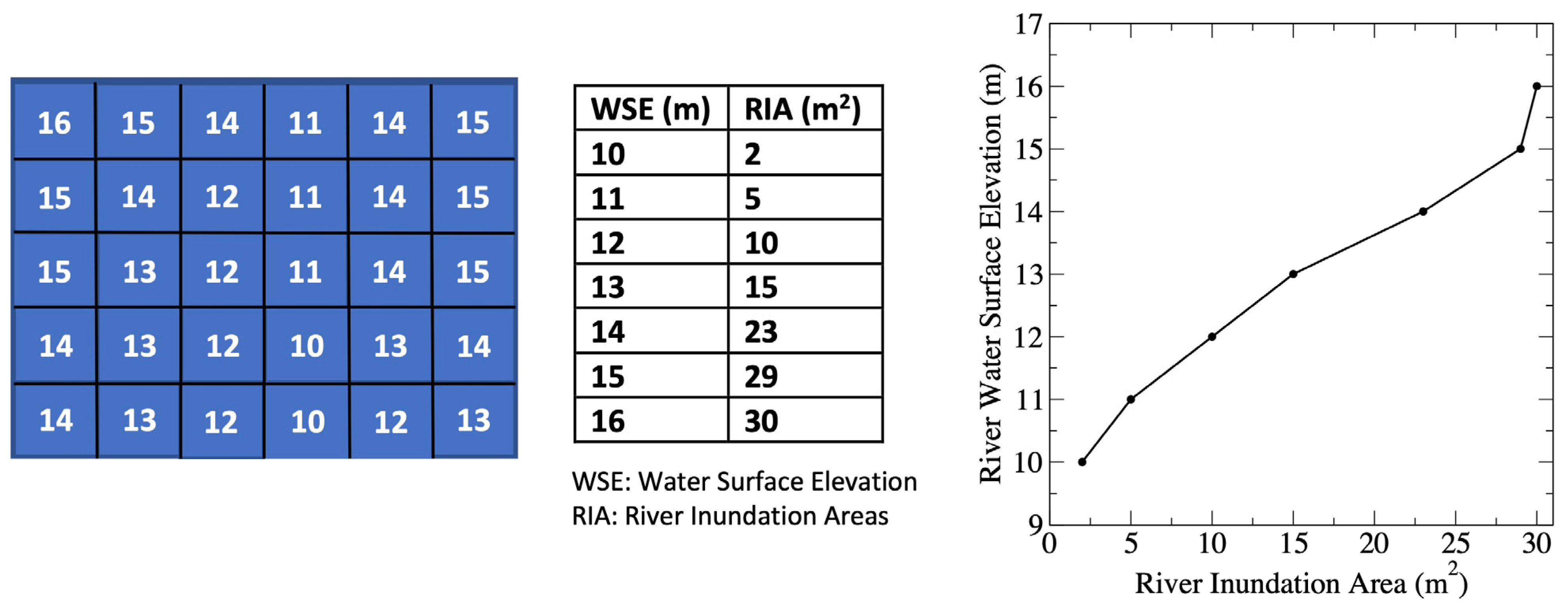
To explain the method of constructing the RIA-WSE rating curves from the TEM data, a hypothetical TEM dataset inside a predefined polygon is shown in
Figure 2. The number within each cell stands for the elevation (in meters) of the riverbank or riverbed, and the grid cell size is 1 m × 1 m. Starting from the minimum elevation (i.e., 10 m) inside the polygon, let river water surface elevation rise toward the maximum elevation inside the polygon (i.e., 16 m) with an incremental interval of 1 m. For a TEM dataset with an elevation precision of 1 cm or 1 mm, an incremental interval of 1 cm or 1 mm should be used. Based on each water surface elevation, the river inundation area (RIA) inside the predefined polygon corresponding to that water surface elevation is calculated. The calculated RIAs are as follows: 2 m
2 (10 m), 5 m
2 (11 m), 10 m
2 (12 m), 15 m
2 (13 m), 23 m
2 (14 m), 29 m
2 (15 m), and 30 m
2 (16 m), where numbers inside the parentheses are the corresponding river WSEs.
Based on the computed RIAs, a RIA-WSE rating curve is constructed and plotted in
Figure 2. Actually, a RIA-WSE look-up table might be more useful than a RIA-WSE rating curve for determining river WSEs. For example, if the
RIA extracted from Landsat imagery is between
RIAi and
RIAi+1, we can use the linear interpolation to estimate the WSE as follows:
where
WSEi and
WSEi+1 are WSEs corresponding to
RIAi and
RIAi+1, respectively.
3.3. Twenty Water Indices
The commonly used water indices are green band based [
61] and include the normalized difference water index (
NDWI) [
62], the modified normalized difference water index (MNDWI) [
63], and the automatic water extraction index for non-shadows (
AWEIns) and shadows (
AWEIs) [
64]. The formulas of these five water indices are given as follows:
where
rG rNIR,
rSWIR1,
rSWIR2,
rB are spectral reflectance of green, near-infrared, shortwave-infrared 1, shortwave-infrared 2 and blue bands, respectively. Pan et al. (2020) suggested that the ultra-blue, blue, and red bands of the Landsat 8 and 9 OLI imagery could also be used in computing water index [
61], as the blue or ultra-blue band might work better for clear water and the red band for water containing a large amount of sediments. Therefore, if all four visible light bands of Landsat 8 and 9 OLI imagery are used to compute the water index, twenty water indices can be yielded as follows:
where
rV is the spectral reflectance of one of four visible light bands, i.e., ultra-blue (
rUB), blue (
rB), green (
rG), and red (
rR).
3.4. The Otsu Method
In this study, the Otsu method [
65], an unsupervised image classification method, was used to determine the optimal water index threshold for differentiating water and non-water pixels in Landsat 8–9 OLI imagery. The principle of the Otsu method is to determine the optimal water index threshold for maximizing an objective function given as follows:
where
Pw and
Pnw are probabilities of water and non-water pixels, respectively, and
μw and
μnw are mean water index values of water and non-water pixels, respectively. The optimal water index threshold (OWI) is determined by iterating the water index threshold between −1 and 1 with an interval of 0.01 to achieve the maximum value of the objective function, as shown in Equation (8). All terms on the right-hand side of Equation (8) are computed as follows:
where
WIi is the water index of pixel
i,
n,
nw,
nnw are the number of total pixels, the number of pixels with a water index greater than OWI, and the number of pixels with a water index less than or equal to OWI, inside the predefined polygon, respectively.
3.5. Resample Landsat 8–9 OLI Imagery
The spatial resolution of Landsat 8–9 OLI imagery is 30 m, which is much coarser than the spatial resolution of the TEM data (i.e., 1 m) used in this study for constructing the RIA-WSE rating curves. To reduce errors and uncertainty in the extracted RIAs from the Landsat 8–9 OLI imagery due to the coarse resolution of the Landsat 8–9 OLI imagery, two raster resampling methods (bilinear and cubic) embedded in the ArcGIS Pro software 3.3 were used to resample each Landsat 8–9 OLI imagery from the cell size of 30 m to 1 m.
3.6. Accuracy Assessment
To assess the accuracy of the estimated river WSEs, the measured river WSEs at the time close to the scene center times of the Landsat 8–9 OLI images used for extracting river inundation areas were used for computing the errors (i.e., WSE
est − WSE
obs). For the NAIP imagery, the measured river WSEs at 12:00 pm local standard time were used to compute the errors in the estimated WSEs from the NAIP imagery since most NAIP images were collected between 10:00 am and 2:00 pm local standard time [
66]. Since only the daily mean WSE data are available at the Wabasha station operated by the U.S. Army Corps of Engineers, the observed daily mean WSEs were used to compute the errors.
3.7. The K-Nearest Neighbor (KNN) Method
Since no metadata of the NAIP aerial photos downloaded from the USGS EarthExplorer is available for converting the digital number (DN) of each pixel into all required spectral reflectance for computing all twenty water indices described in
Section 3.3, the K-Nearest Neighbor (KNN) classifier [
67], a supervised image classification method, was used for identifying water and non-water pixels in the NAIP aerial photos. Applying the KNN method to determine if an unknown pixel x belongs to water or non-water class, two training sample sets (i.e., water and non-water) are selected first, and then the spectral distance in the near-infrared band of the NAIP imagery between pixel x and each training pixel is computed. The sum of the inverse distances between pixel x and all water training pixels (SID
w) is compared with the sum of the inverse distance between pixel x and all non-water training pixels (SID
nw). If SID
w > SID
nw, pixel x belongs to the water class; otherwise, x belongs to the non-water class [
56]. After the RIAs inside the predefined polygon were computed, they were used to estimate WSEs based on the constructed RIA-WSE rating curves.
4. Results
4.1. Construction of the RIA-WSE Rating Curves
4.1.1. Grafton
The USGS gauging station 05587450 along the Mississippi River at Grafton, Illinois, is located at (East 722,743 m, North 4,316,370 m, UTM15) and shown as a red dot in
Figure 3a (NAIP) and
Figure 3b (Topobathy). The red polygon shown in
Figure 3a,b is the polygon for constructing the RIA-WSE rating curve with an area of 58,116 m
2 (about 65 pixels in Landsat 8–9 OLI imagery). The constructed RIA-WSE rating curve is plotted in
Figure 3c.
4.1.2. Prescott
The USGS gauging station 05344500 along the Mississippi River at Prescott, Wisconsin, is located at East 515,817 m, North 4,954,732 m, UTM15 and shown as a red dot in
Figure 4a (NAIP) and
Figure 4b (Topobathy). A polygon with an area of 19,028 m
2 (about 21 pixels in Landsat 8–9 OLI imagery) for constructing the RIA-WSE rating curve was chosen over the gauging station shown as a red polygon in
Figure 4a,b. The constructed RIA-WSE rating curve is plotted in
Figure 4c.
4.1.3. Red Wing
The USGS gauging station 05355250 along the Mississippi River at Red Wing, Minnesota, is located at (East 536,330 m, North 4,934,762 m, UTM15) and shown as a red dot in
Figure 5a (NAIP) and
Figure 5b (Topobathy). This gauging station is located around an area with some man-made structures. To reduce the impact of man-made structures on the extracted RIAs inside the polygon, a polygon with an area of 33,356 m
2 (about 37 pixels in Landsat 8–9 OLI imagery) was chosen at the opposite riverbank shown as a red polygon in
Figure 5a,b. It is to be noted that the dense plant canopy in this selected polygon might impact the estimated WSEs at high flow conditions. The constructed RIA-WSE rating curve is plotted in
Figure 5c.
4.1.4. St. Louis
The USGS gauging station 07010000 along the Mississippi River at St. Louis, Missouri, is located at (East 745,505 m, North 4,279,369 m, UTM15) and shown in
Figure 6a (NAIP) and
Figure 6b (Topobathy) as a red dot. This gauging station is located near a bridge. To reduce the impact of the bridge in the extracted RIAs from Landsat imagery, a polygon with an area of 65,379 m
2 (about 73 pixels in Landsat 8–9 OLI imagery) was chosen downstream of the gauging station shown as a red polygon in
Figure 6a,b. The constructed RIA-WSE rating curve is plotted in
Figure 6c.
4.1.5. Wabasha
The USACE gauging station along the Mississippi River at Wabasha, Minnesota, is located at (East 576,708 m, North 4,915,333 m, UTM15) and is shown as a red dot in
Figure 7a (NAIP) and
Figure 7b (Topobathy). This gauging station is located around an area with some man-made structures. To reduce the impact of man-made structures, a polygon with an area of 19,044 m
2 (about 21 pixels in Landsat 8–9 OLI imagery) was chosen upstream of the gauging station shown as a red polygon in
Figure 7a,b. The constructed RIA-WSE rating curve is plotted in
Figure 7c.
4.1.6. Winona
The USGS gauging station 05378500 along the Mississippi River at Winona, Minnesota, is located at (East 609,136 m, North 4,878,946 m, UTM15) and shown in
Figure 8a (NAIP) and
Figure 8b (Topobathy) as a red dot. This gauging station is located around an area with some man-made structures. To reduce the impact of man-made structures, a polygon with an area of 46,283 m
2 (about 51 pixels in Landsat 8–9 OLI imagery) was chosen slightly downstream of the gauging station shown as a red polygon in
Figure 8a,b. The constructed RIA-WSE rating curve is plotted in
Figure 8c.
4.2. Comparison of the Bilinear and Cubic Resampling Methods
In this study, the topobathymetric elevation model (TEM) data used for constructing the RIA-WSE rating curves has a spatial resolution of 1 m, while the spatial resolution of Landsat 8–9 OLI imagery is 30 m. To match the finer resolution of the TEM data, all Landsat images used in this study were resampled (downscaled) from 30 m to 1 m using two resampling methods in the ArcGIS Pro, i.e., bilinear and cubic.
Table 2 shows that among the six selected stations, the percentage of the estimated WSEs from the resampled Landsat 8–9 OLI imagery using the cubic resampling method being more accurate than the estimated WSEs using the bilinear resampling method ranged from 58.3% (Red Wing) to 86.8% (St. Louis), which indicates that the cubic resampling method is better than the bilinear resampling method in terms of the accuracy of the estimated WSEs based on the extracted RIAs from the resampled Landsat 8–9 OLI imagery. The reason why the cubic resampling method is better than the bilinear resampling method for downscaling Landsat 8–9 OLI imagery from 30 m to 1 m might be that the cubic resampling method has one more parameter than the bilinear method.
4.3. Comparison of the Estimated WSEs among Twenty Water Indices
As described in
Section 3.3, there are twenty water indices that can be used for differentiating water and non-water pixels in Landsat 8–9 OLI imagery. Two criteria were employed in this study to compare these twenty water indices. First, at each station, the estimated WSEs using the twenty water indices were ranked from 1, which is associated with the smallest error (compared with the observed WSEs), to 20 (the largest error) for each of the selected Landsat 8–9 OLI images. Then, these ranking data were used for making the box plots, as shown in
Figure 9 (bilinear resampling) and
Figure 10 (cubic resampling).
The second criterion for evaluating twenty water indices is the box plot of the errors in the estimated WSEs at each station, as shown in
Figure 11 (bilinear resampling) and
Figure 12 (cubic resampling).
Figure 9,
Figure 10,
Figure 11 and
Figure 12 all demonstrate that the automatic water extraction index for non-shadows (AWEIns). The shadows (AWEIs) are better than other water indices in terms of the accuracy of the estimated WSEs at all six selected stations, no matter if the bilinear resampling method or the cubic resampling method was used to downscale the Landsat 8–9 OLI imagery from 30 m to 1 m.
5. Discussion
5.1. Comparison of the Estimated WSEs between AWEIns and AWEIs
According to the results presented in
Section 4.3, AWEIns and AWEIs are better than other water indices in terms of the accuracy of the estimated WSEs. It is necessary to determine which one is better, AWEIns or AWEIs. To compare the performance of AWEIns and AWEIs, percentages of the absolute errors in the estimated WSEs using AWEIns that are equal to (i.e., |err|
AWEIns = |err|
AWEIs), less than (i.e., |err|
AWEIns < |err|
AWEIs), and greater than (i.e., |err|
AWEIns > |err|
AWEIs) the absolute errors in the estimated WSEs using AWEIs at each of six selected stations were computed and listed in
Table 3. Among these six stations, only the station at St. Louis exhibited that more than 50% of the absolute errors in the estimated WSEs using AWEIns are less than that of AWEIs, and the other five stations all showed that AWEIs performed better than AWEIns, which are attributed mainly to more or fewer shadows existed in the predefined polygons at the six selected gauging stations. These results are consistent with other studies, e.g., [
61,
64,
68].
5.2. Comparison of the Estimated WSEs among Four AWEIs
Since four visible light bands (i.e., ultra-blue, blue, green, and red) were used in this study for computing the automatic water extraction index for shadows (AWEIs), while AWEIs performed better than other water indices, it is necessary to compare the errors in the estimated WSEs among these four visible light band-based AWEIs.
Table 4 lists the percentages of the absolute errors in the estimated WSEs associated with each of the AWEIs that are the smallest among the four visible light band-based WAEIs at each station.
It should be noted that the sum of the percentages of the smallest absolute errors among four visible light band-based AWEIs at each station is not necessarily equal to 100% because multiple visible light band-based AWEIs could yield the same lowest absolute errors at the same time.
According to
Table 4, either ultra-blue or red band-based AWEIs performed better than blue or green band-based AWEIs in terms of the accuracy of the estimated WSEs from Landsat 8–9 OLI imagery, although the green band-based water indices are commonly used.
This study [
61] suggested that the ultra-blue band might work better than other visible light bands for clear water, and the red band might perform well for water with a large amount of sediments.
Table 4 only shows the overall performance of AWEIs among 60–80 imaging dates during the period of 2013–2024. We understand that water quality is a dynamic variable that varies with time, atmospheric conditions, weather patterns, land use and land cover change, and others. To reveal the water quality impact on the performance of four visible light band-based AWEIs, the suspended sediment concentration data collected at the St. Louis station (only this station has daily water quality data during a portion of this study period) were used to make a time series plot as shown in
Figure 13. The absolute errors of the estimated WSEs by the four AWEIs versus time were also plotted in
Figure 13.
Figure 13 shows that at St. Louis station, most of the estimated WSEs using the ultra-blue band-based AWEIs are more accurate than the estimated WSEs using the other three visible light band-based AWEIs, which is consistent with
Table 4.
Figure 13 also shows that as the suspended sediment concentration decreased, the difference in the absolute errors of the estimated WSEs between red and ultra-blue band-based AWEIs increased, especially on 25 July 2013. This result suggests that the red band-based AWEIs work better for water with high sediment loads, while the ultra-blue band-based AWEIs are suitable for clear water.
5.3. The Dependence of the Errors in the Estimated WSEs by AWEIns and AWEIs on River Stages
To investigate how the errors in the estimated WSEs by AWEIns and AWEIs vary with river stages, the scatter plots of measured WSEs versus estimated WSEs using AWEIns and AWEIs are illustrated in
Figure 14, along with the constructed RIA-WSE rating curve at each station. Four colored dots, i.e., cyan, blue, green, and red in
Figure 14, represent estimated WSEs using ultra-blue, blue, green and red band-based AWEIns or AWEIs, respectively.
Figure 14 shows that overall AWEIs performed better than AWEIns, especially at Winona station, which is consistent with
Table 3. Since AWEIs are better than AWEIns, let us focus on the AWEIs results in
Figure 14. To understand the error behavior of the estimated WSEs using the AWEIs, the scatter plots of the measured WSEs versus the estimated WSEs from the NAIP imagery at each station were also plotted in the same plots of the AWEIs results in
Figure 14.
Figure 14 shows that at Grafton station, as WSEs above 129 m, the estimated WSEs are more accurate than those below 129 m. The constructed RIA-WSE rating curve at Grafton plotted in
Figure 14 exhibits a sharp increase in the slope as the WSE drops below 129 m, i.e., a small change in RIA is associated with a large change in WSE. This sharp increase in the slope of the RIA-WSE rating curve could induce uncertainty in the extracted RIAs from Landsat 8–9 OLI imagery, although Landsat 8–9 OLI images used in this study were downscaled from 30 m to 1 m. The black dots shown in
Figure 14 at Grafton do not show the same error behavior as the Landsat results because the NAIP imagery has a spatial resolution of 1 m prior to 2018 and 0.6 after 2018.
At Prescott station, the estimated WSEs were more accurate as the WSEs above 207 m than those below 207 m due to a slight increase in the slope of the constructed RIA-WSE rating curve. No NAIP imagery was acquired during the time as the WSE was below 207 m. The estimated WSEs based on NAIP imagery at Prescott as WSE below 207 m are more accurate than the Landsat results, as shown in
Figure 14.
At Red Wing station, the errors in the estimated WSEs from Landsat imagery as WSE below 205 m are due to the steep slope in the constructed RIA-WSE rating curve, and the errors in the Landsat estimated WSEs as WSE above 205 m are probably caused by the dense plant canopy cover (see
Figure 6a) that blocks remote sensing of water on the ground and in turn decreases the extracted RIAs from the Landsat 8–9 OLI imagery. The NAIP results shown in
Figure 14 are better than the Landsat results as WSE below 205 m. There is no NAIP imagery acquired at the time as WSE above 205 m.
Results at St. Louis, Wabasha and Winona all demonstrate that a sharp increase in the constructed RIA-WSE rating curves could increase the errors of the Landsat estimated WSEs, especially at St. Louis station as WSE below 108 m, while such impact did not appear in the estimated WSEs from NAIP imagery (unfortunately no NAIP images are available at St. Louis as WSE below 108 m), and the main reason is that the NAIP imagery has a very high spatial resolution, although the Landsat imagery was resampled from 30 m to 1 m in this study.
6. Conclusions
This study has demonstrated that the topobathymetric elevation model (TEM) data are more useful than the DEM data in constructing the RIA-WSE rating curves because the constructed RIA-WSE rating curves from the TEM data can be used for estimating river WSEs over the whole dynamic range of the river stages especially at the low flow conditions, while the constructed RIA-WSE rating curves from the DEM data are only valid above the minimum elevations in the DEM data at river cross-sections, which actually are the water surface elevations as the ground survey was conducted collecting elevation data for producing DEM data. However, TEM data are not currently available globally, which could hamper the application of the method developed in this study to river WSE estimations from remotely sensed river inundation areas. Therefore, the author of this study strongly advocates that more efforts are needed to produce the TEM data covering major global rivers in the near future, and eventually all rivers in the world, including the first-order streams.
The selection of a polygon for constructing the RIA-WSE rating curve is critical; as shown in this study, an optimal polygon should cover the riverbank and a portion of the river without any man-made structures and dense vegetation cover. High spatial resolution satellite (e.g., Google Earth Images) or aerial imagery (e.g., NAIP) is very useful for choosing an optimal polygon to construct the RIA-WSE rating curve. However, sometimes, we may need to choose a polygon far away from the cross-section of interest; as the distance from the cross-section increases, the errors in the estimated WSEs would also increase since the water surface elevation can vary significantly along the river, especially during high flow conditions. If this is the case, the direct method seems a better choice as the radar altimeter or laser scanning points can directly strike the water surface.
As Landsat imagery has a spatial resolution of 30 m, to improve the accuracy of the estimated WSEs, resampling or downscaling Landsat imagery is necessary. This study found that the cubic resampling method is better than the bilinear resampling method in terms of the accuracy of the Landsat-estimated WSEs. If the slope in the RIA-WSE rating curve is not very steep, and there is no dense vegetation cover in the predefined polygon, the resampled Landsat imagery could yield highly accurate results. However, it might be difficult for the Landsat imagery to achieve a centimeter-level accuracy in the estimated WSEs, as the WSE is at the range wherein the slope in the constructed RIA-WSE rating curve is steep, which is one of the major limitations of the method developed in this study. Under these river stage conditions, high-resolution imagery (e.g., Sentinel satellites, UAV images) is needed to accurately estimate WSEs.
Another limitation associated with Landsat imagery stems from the optical remote sensing characteristics of the Landsat 8/9 OLI. Compared to optical remote sensing, microwave remote sensing has all weather and night operational capability. Such advantages associated with microwave remote sensing greatly increase available remotely sensed data/imagery for mapping river inundation areas [
69,
70], especially in the cloudiest areas (e.g., tropical rainforest, monsoon regions during rainy seasons) and high latitudes during winter seasons. A future study is necessary to apply microwave remote sensing data to estimate river WSEs using the constructed RIA-WSE rating curves.
The results of this study demonstrate that in addition to the green band-based water indices, three other visible light bands (i.e., ultra-blue, blue, and red) in the Landsat 8–9 OLI imagery can also be used to compute the water index. Although the green band-based water indices are commonly used in the literature, this study showed that the ultra-blue or red band-based AWEIs performed better in terms of the accuracy of the estimated WSEs from Landsat 8–9 OLI imagery.
Funding
This research received no external funding.
Data Availability Statement
All data used in this study are available to everyone through email communication with the author (feifei.pan@unt.edu). After the author receives the request for data, the author will share the data with the requester via Google Drive and send the link to the requester.
Acknowledgments
The author thanks the Upper Mississippi River System (UMRS) for producing the topobathymetric elevation model (TEM) data along the Upper Mississippi River and making the TEM data available to the public, and the three anonymous reviewers for providing constructive comments to improve this study.
Conflicts of Interest
The author declares no conflicts of interest.
References
- Buchanan, T.J.; Somers, W.P. Discharge measurements at gaging stations. In Techniques for Water Resources Investigation of the United States Geological Survey; U.S. Geological Survey: Reston, VA, USA, 1969; Book 3, Chapter A8. [Google Scholar]
- Olson, S.A.; Norris, J.M. U.S. Geological Survey Streamgaging; Fact Sheet, 2005–3131; U.S. Geological Survey: Reston, VA, USA, 2007.
- Abbott, B.W.; Bishop, K.; Zarnetske, J.P.; Minaudo, C.; Chapin, F.S., III; Krause, S.; Hannah, D.M.; Conner, L.; Ellison, D.; Godsey, S.E.; et al. Human domination of the global water cycle absent from depictions and perceptions. Nat. Geosci. 2019, 12, 533–540. [Google Scholar] [CrossRef]
- Gleeson, T.; Wang-Erlandsson, L.; Porkka, M.; Zipper, S.C.; Jaramillo, F.; Gerten, D.; Fetzer, I.; Cornell, S.E.; Piemontese, L.; Gordon, L.J.; et al. Illumination water cycle modifications and Earth system resilience in the Anthropocene. Water Resour. Res. 2020, 56, e2019WR024957. [Google Scholar] [CrossRef]
- Hamed, K.; Rao, A.R. Flood Frequency Analysis, 1st ed.; CRC Press: Boca Raton, FL, USA, 2000; p. 376. [Google Scholar]
- Bhat, M.S.; Alam, A.; Ahmad, B.; Katlia, B.S.; Farooq, H.; Taloor, A.K.; Ahmad, S. Flood frequency analysis of river Jhelum in Kashmir basin. Quat. Int. 2019, 507, 288–294. [Google Scholar] [CrossRef]
- Faulkner, D.; Warren, S.; Spencer, P.; Sharkey, P. Can we still predict the future from the past? Implementing non-stationary flood frequency analysis in the UK. J. Flood Risk Manag. 2019, 13, e12582. [Google Scholar] [CrossRef]
- Bischiniotis, K.; de Moel, H.; van den Homberg, M.; Couasnon, A.; Aerts, J.; Nobre, G.G.; Zsoter, E.; van den Hurk, B. A framework for comparing permanent and forecast-based flood risk-reduction strategies. Sci. Total Environ. 2020, 720, 137572. [Google Scholar] [CrossRef]
- Speight, L.J.; Cranston, M.D.; White, C.J.; Kelly, L. Operational and emerging capabilities for surface water flood forecasting. Wiley Interdiscip. Rev. Water 2021, 8, e1517. [Google Scholar] [CrossRef]
- Jain, S.K.; Singh, V.P. Water Resources Systems Planning and Management, 2nd ed.; Elsevier: Amsterdam, Netherlands, 2023; p. 893. [Google Scholar]
- Niu, W.; Feng, Z. Evaluating the performances of several artificial intelligence methods in forecasting daily streamflow times series for sustainable water resources management. Sustain. Cities Soc. 2021, 64, 102562. [Google Scholar] [CrossRef]
- Grizzetti, B.; Liquete, C.; Pistocchi, A.; Vigiak, O.; Zulian, G.; Bouraoui, F.; De Roo, A.; Cardoso, A.C. Relationship between ecological condition and ecosystem services in European rivers, lakes and coastal waters. Sci. Total Environ. 2019, 671, 452–465. [Google Scholar] [CrossRef]
- Suwal, N.; Huang, X.; Kuriqi, A.; Chen, Y.; Pandey, K.P.; Bhattarai, K.P. Optimisation for cascade reservoir operation considering environmental flows for different environmental management classes. Renew. Energy 2020, 158, 453–464. [Google Scholar] [CrossRef]
- Zhang, S.; Jing, Z.; Li, W.; Wang, L.; Liu, D.; Wang, T. Navigation risk assessment method based on flow conditions: A case study of the river reach between the Three Gorge Dam and the Gezhouba Dam. Ocean Eng. 2019, 175, 71–79. [Google Scholar] [CrossRef]
- Kwon, S.; Seo, I.; Kim, B.; Jung, S.; Kim, Y. Assessment of river recreation safety using spatial river recreational index by integration of hydrodynamic model and fuzzy logic. Res. Sq. 2023. [Google Scholar] [CrossRef]
- Fekete, B.M.; Vörösmarty, C.J. The current status of global river discharge monitoring and potential new technologies complementing traditional discharge measurements. In Proceedings of the PUB Kick-Off Meeting, Brasilia, Brazil, 20–22 November 2002; IAHS Publication: Wallingford, UK, 2007; p. 309. [Google Scholar]
- Vörösmarty, C.J.; Willmott, C.J.; Choudhyry, B.J.; Scholss, A.L.; Stearns, T.K.; Robeson, S.M.; Dorman, T.J. Analyzing the discharge regime of a large tropical river through remote sensing, ground-based climatic data and modeling. Water Resour. Res. 1996, 32, 3137–3150. [Google Scholar] [CrossRef]
- IAHS Ad Hoc Committee. Global Water Data: A newly endangered species. EOS Trans. Am. Geophys. Union 2001, 82, 54–58. [Google Scholar] [CrossRef]
- Bjerklie, D.M.; Dingman, S.L.; Vörösmarty, C.J.; Holster, C.H.; Congalton, R.G. Evaluating the potential for measuring river discharge from space. J. Hydrol. 2003, 278, 17–38. [Google Scholar] [CrossRef]
- Hannah, D.M.; Demuth, S.; van Lanen, H.A.J.; Looser, U.; Prudhomme, C.; Rees, G.; Stahl, K.; Tallaken, L.M. Large-scale river flow archives: Importance, current status and future needs. Hydrol. Process. 2011, 25, 1191–1200. [Google Scholar] [CrossRef]
- Cloke, H.L.; Pappernberger, F. Ensemble flood forecasting: A review. J. Hydrol. 2009, 375, 613–626. [Google Scholar] [CrossRef]
- Smith, L.C. Satellite remote sensing of river inundation area, stage, and discharge: A review. Hydrol. Process. 1997, 11, 1427–1439. [Google Scholar] [CrossRef]
- Alsdorf, D.E.; Rodriguez, E.; Letternmaier, D.P. Measuring surface water from space. Rev. Geophys. 2007, 45, RG2002. [Google Scholar] [CrossRef]
- Schumann, G.; Bates, P.D.; Horritt, M.S.; Matgen, P.; Pappernberger, F. Progress in integration of remote sensing-derived flood extend and stage data and hydraulic models. Rev. Geophys. 2009, 47, RG4001. [Google Scholar] [CrossRef]
- Pan, F. Remote sensing of river stage and discharge. SPIE Newsroom 2013. [Google Scholar] [CrossRef]
- Pan, F.; Nichols, J. Remote sensing of river stage using the cross sectional inundation area—River stage relationship (IARSR) constructed from digital elevation model data. Hydrol. Process 2013, 27, 3596–3606. [Google Scholar] [CrossRef]
- Pan, F.; Liao, J.; Li, X.; Guo, H. Application of the inundation area-lake level rating curves constructed from the SRTM DEM to retrieving lake levels from satellite measured inundation areas. Comput. Geosci. 2013, 52, 168–176. [Google Scholar] [CrossRef]
- Koblinsky, C.J.; Clarke, R.T.; Brenner, A.C.; Frey, H. Measurement of river level variations with satellite altimetry. Water Resour. Res. 1993, 29, 1839–1848. [Google Scholar] [CrossRef]
- Birkett, C.M.; Mertes, L.A.K.; Dunne, T.; Costa, M.H.; Jasinski, M.J. Surface water dynamics in the Amazon Basin: Application of satellite radar altimetry. J. Geophys. Res.-Atmos. 2002, 107, 8059. [Google Scholar] [CrossRef]
- Coe, M.T.; Birkett, C.M. Calculation of river discharge and prediction of lake height from satellite radar altimetry: Example for the Lake Chad basin. Water Resour. Res. 2004, 40, W10205. [Google Scholar] [CrossRef]
- Kouraev, A.V.; Zakharova, E.A.; Samain, O.; Mognard, N.M.; Cazenave, C. Ob’ river discharge from TOPEX/Poseidon satellite altimetry (1992–2002). Remote Sens. Environ. 2004, 93, 238–245. [Google Scholar] [CrossRef]
- Calmant, S.; Seyler, F. Continental surface waters from satellite altimetry. Comptes Rendus Geosci. 2006, 338, 113–1122. [Google Scholar] [CrossRef]
- Leon, J.G.; Calmant, S.; Seyler, F.; Bonnet, M.P.; Cauhopé, M.; Frappart, F.; Filizola, N.; Fraizy, P. Rating curves and estimation of average water depth at the upper Negro River based on satellite altimeter data and modeled discharges. J. Hydrol. 2006, 328, 481–496. [Google Scholar] [CrossRef]
- Birkinshaw, S.J.; O’Donnell, G.M.; Moore, P.; Kilsby, C.G.; Fowler, H.J.; Berry, P.A.M. Using satellite altimetry data to augment flow estimation techniques on the Mekong River. Hydrol. Process. 2010, 24, 3811–3825. [Google Scholar] [CrossRef]
- Bhang, K.J.; Schwartz, F.W.; Park, S. Estimating historic lake stages from one-time snapshot, the Shuttle Radar Topography Mission of 2020. Hydrol. Process. 2010, 34, 1834–1843. [Google Scholar] [CrossRef]
- Altenau, E.H.; Pavelsky, T.M.; Moller, D.; Pitcher, L.H.; Batest, P.D.; Durand, M.T.; Smith, L.C. Temporal variations in river water surface elevation and slope captured by AirSWOT. Remote Sens. Environ. 2019, 224, 304–316. [Google Scholar] [CrossRef]
- Chipman, J.W. A multisensory approach to satellite monitoring of trends in lake area, water level and volume. Remote Sens. 2019, 11, 158. [Google Scholar] [CrossRef]
- Jiang, L.; Andersen, O.B.; Nielsen, K.; Zhang, G.; Bauer-Gottwein, P. Influence of local geoid variation on water surface elevation estimates derived from multi-mission altimetry for Lake Namco. Remote Sens. Environ. 2019, 221, 65–79. [Google Scholar] [CrossRef]
- Li, X.; Long, D.; Huang, Q.; Han, P.; Zhao, F.; Wada, Y. High-temporal-resolution water level and storage change data sets for lakes on the Tibetan Plateau during 2000–2017 using multiple altimetric missions and Landsat-derived lake shoreline positions. Earth Syst. Sci. Data 2019, 11, 1603–1627. [Google Scholar] [CrossRef]
- Ma, Y.; Xu, N.; Sun, J.; Wang, X.; Yang, F.; Li, S. Estimating water levels and volumes of lakes dated back to the 1980s using Landsat imagery and photon-counting lidar datasets. Remote Sens. Environ. 2019, 212, 111287. [Google Scholar] [CrossRef]
- Zhang, G.; Chen, W.; Xie, H. Tibetan Plateau’s lake level and volume changes from NASA’s ICESat/ICESat-2 and Landsat Missions. Geophys. Res. Lett. 2019, 46, 13107–13118. [Google Scholar] [CrossRef]
- Bandini, F.; Sunding, T.P.; Linde, J.; Smith, O.; Jensen, I.K.; Koppl, C.J.; Butts, M.; Bauer-Gottwein, P. Unmanned aerial system (UAS) observations of water surface elevation in a small stream: Comparison of radar altimetry, Lidar and photogrammetry techniques. Remote Sens. Environ. 2020, 237, 111487. [Google Scholar] [CrossRef]
- Tortini, R.; Noujdina, N.; Yeo, S.; Ricko, M.; Birkett, C.; Khandelwal, A.; Kumar, V.; Marlier, M.A.E.; Lettenmaier, D.P. Satellite-based remote sensing data set of global surface water storage change from 1992 to 2018. Earth Syst. Sci. Data 2020, 12, 1141–1151. [Google Scholar] [CrossRef]
- Yuan, C.; Gong, P.; Bai, Y. Performance assessment of ICESat-2 laser altimeter data for water level measurement over lakes and reservoirs in China. Remote Sens. 2020, 12, 770. [Google Scholar] [CrossRef]
- Frappart, F.; Blarel, F.; Fayad, I.; Berge-Nguyen, M.; Crétaus, J.F.; Shu, S.; Schregenberger, J.; Badhdadi, N. Evaluation of the performances of radar and lidar altimetry mission for water level retrievals in mountainous environment: The case of the Swiss lakes. Remote Sens. 2021, 13, 2196. [Google Scholar] [CrossRef]
- Wu, G.; Liu, Y.; Liu, R. Assessing the performance of the Tianggong-2 wide-swath imaging altimeter observations for water level monitoring over complex and shallow lake. J. Hydrol. 2022, 612, 128164. [Google Scholar] [CrossRef]
- Hamilton, S.K.; Sipple, S.J.; Melack, J.M. Inundation patterns in the Pantanal wetland of South America determined from passive microwave remote sensing. Arch. Hydrobiol. 1996, 137, 115–141. [Google Scholar] [CrossRef]
- Brakenridge, G.R.; Tracy, B.T.; Knox, J.C. Orbital SAR remote sensing of a river flood wave. Int. J. Remote Sens. 1998, 19, 1439–1445. [Google Scholar] [CrossRef]
- Pietroniro, A.; Prowse, T.; Peters, D.L. Hydrologic assessment of an inland freshwater data using multi-temporal satellite remote sensing. Hydrol. Process. 1999, 13, 2483–2498. [Google Scholar] [CrossRef]
- Al-Khudhairy, D.H.A.; Leemhuis, C.; Hoffmann, V.; Shepherd, I.M.; Calaon, R.; Thompson, J.R.; Gavin, H.; Casca-Tucker, D.L.; Zalidis, G.; Bilas, G.; et al. Monitoring wetland ditch water levels using Landsat TM and ground-based measurements. Photogramm. Eng. Remote Sens. 2002, 68, 809–818. [Google Scholar]
- Temimi, M.; Leconte, R.; Brissette, F.; Chaouch, N. Flood monitoring over the Mackenzie River Basin using passive microwave data. Remote Sens. Environ. 2005, 98, 344–355. [Google Scholar] [CrossRef]
- Matgen, P.; Schumann, G.; Henry, J.P.; Hoffmann, L.; Pfister, L. Integration of SAR-derived river inundation areas, high-precision topographic data and a river flow model toward near real-time flood management. Int. J. Appl. Earth Obs. Geoinf. 2007, 9, 247–263. [Google Scholar] [CrossRef]
- Schumann, G.; Pappernberger, F.; Matgen, P.; Pappenberger, F. Estimating uncertainty associated with water stages from a single SAR image. Adv. Water Resour. 2008, 31, 1038–1047. [Google Scholar] [CrossRef]
- Schumann, G.; Pappernberger, F.; Matgen, P. Conditioning water stages from satellite imagery on uncertain data points. IEEE Geosci. Remote Sens. Lett. 2008, 5, 810–813. [Google Scholar] [CrossRef]
- Smith, L.C.; Pavelsky, T.M. Remote sensing of volumetric storage changes in lakes. Earth Surf. Process. Landf. 2009, 34, 1353–1358. [Google Scholar] [CrossRef]
- Pan, F.; Wang, C.; Xi, X. Constructing river stage-discharge rating curves using remotely sensed river cross-sectional inundation areas and river bathymetry. J. Hydrol. 2016, 540, 670–687. [Google Scholar] [CrossRef]
- Dong, Y.; Fan, L.; Zhao, J.; Huang, S.; Geiß, C.; Wang, L.; Taubenböck, H. Mapping of small water bodies with integrated spatial information for time series images of optical remote sensing. J. Hydrol. 2022, 614, 128580. [Google Scholar] [CrossRef]
- Kebede, M.G.; Wang, L.; Li, X.; Hu, Z. Remote sensing-based river discharge estimation for a small river flowing over the high mountain regions of the Tibetan Plateau. Int. J. Remote Sens. 2019, 41, 3322–3345. [Google Scholar] [CrossRef]
- Stone, J.M.; Hanson, J.L.; Sattler, S.R. The Upper Mississippi River System-Topobathy; Fact Sheet, 2016–3097; U.S. Geological Survey: Reston, VA, USA, 2017; 4p. [CrossRef]
- Rogala, J.T. Methodologies Employed for Bathymetric Mapping and Sediment Characterization as Part of the Upper Mississippi River System Navigation Feasibility Study; ENV Report 13, Interim Report for the Upper Mississippi River—Illinois Waterway System Navigation Study; U.S. Army Engineers District: Rock Island, IL, USA; St. Louis, MO, USA; St. Paul, MN, USA, 1999. [Google Scholar]
- Pan, F.; Xi, X.; Wang, C. A comparative study of water indices and image classification algorithms for mapping inland surface water bodies using Landsat imagery. Remote Sens. 2020, 12, 1611. [Google Scholar] [CrossRef]
- McFeeters, S.K. The use of the normalized difference water index (NDWI) in the delineation of open water features. Int. J. Remote Sens. 1996, 17, 1425–1432. [Google Scholar] [CrossRef]
- Xu, H. Modification of normalized difference water index (NDWI) to enhance open water features in remotely sensed imagery. Int. J. Remote Sens. 2006, 27, 3025–3033. [Google Scholar] [CrossRef]
- Feyisa, G.L.; Meilby, H.; Fensholt, R.; Proud, S.R. Automated water extraction index: A new technique for surface water mapping using Landsat imagery. Remote Sens. Environ. 2014, 140, 23–35. [Google Scholar] [CrossRef]
- Otsu, N. A threshold selection method from gray-level histograms. IEEE Trans. Syst. Mancybernetics 1979, 9, 62–69. [Google Scholar] [CrossRef]
- Bunis, L.; Mootz, J. Aerial Photography Field Office—National Agriculture Imagery Program (NAIP) Suggested Best Practices–Final Report; 2007; Performed for USDA under Contract: CDRL A006 Submitted under GSA Contract Number GS-23F-0284M, SIN 871_2. Available online: https://www.fsa.usda.gov/Internet/FSA_File/naip_best_practice.pdf (accessed on 6 August 2024).
- Richards, J.A. Remote Sensing Digital Image Analysis: An Introduction, 5th ed.; Springer: Berlin/Heidelberg, Germany, 2013; p. 494. [Google Scholar]
- Fisher, A.; Flood, N.; Danaher, T. Comparing Landsat water index methods for automated water classification in eastern Australia. Remote Sens. Environ. 2016, 175, 167–182. [Google Scholar] [CrossRef]
- Prigent, C.; Jimenez, C.; Bousquet, P. Satellite-derived global surface water extent and dynamics over the last 25 years (GIEMS-2). J. Geophys. Res.-Atmos. 2019, 125, e2019JD030711. [Google Scholar] [CrossRef]
- Yan, Q.; Liu, S.; Chen, T.; Jin, S.; Xie, T.; Huang, W. Mapping surface water fraction over the Pan-Tropilca region using CYGNSS data. IEEE Trans. Geosci. Remote Sens. 2024, 62, 5800914. [Google Scholar] [CrossRef]
Figure 1.
Flowchart of the overall method used in this study contains three sections: (1) constructing the RIA-WSE rating curves inside the predefined polygons over or near gauging stations (upper left section); (2) computing river inundation areas inside the predefined polygons and estimating river water surface elevations (upper right section); and (3) evaluating the curacy of the estimated WSEs (bottom section).
Figure 2.
Constructing the RIA-WSE from hypothetical TEM data.
Figure 2.
Constructing the RIA-WSE from hypothetical TEM data.
Figure 3.
(a) NAIP image (left), (b) topobathy image (center), and (c) constructed RIA-WSE rating curve (right) at Grafton.
Figure 3.
(a) NAIP image (left), (b) topobathy image (center), and (c) constructed RIA-WSE rating curve (right) at Grafton.
Figure 4.
(a) NAIP image (left), (b) topobathy image (center), and (c) constructed RIA-WSE rating curve (right) at Prescott.
Figure 4.
(a) NAIP image (left), (b) topobathy image (center), and (c) constructed RIA-WSE rating curve (right) at Prescott.
Figure 5.
(a) NAIP image (left), (b) topobathy image (center), and (c) constructed RIA-WSE rating curve (right) at Red Wing.
Figure 5.
(a) NAIP image (left), (b) topobathy image (center), and (c) constructed RIA-WSE rating curve (right) at Red Wing.
Figure 6.
(a) NAIP image (left), (b) Topobathy image (center), (c) Constructed RIA-WSE rating curve (right) at St. Louis.
Figure 6.
(a) NAIP image (left), (b) Topobathy image (center), (c) Constructed RIA-WSE rating curve (right) at St. Louis.
Figure 7.
(a) NAIP image (left), (b) Topobathy image (center), (c) Constructed RIA-WSE rating curve (right) at Wabasha.
Figure 7.
(a) NAIP image (left), (b) Topobathy image (center), (c) Constructed RIA-WSE rating curve (right) at Wabasha.
Figure 8.
(a) NAIP image (left), (b) topobathy image (center), (c) constructed RIA-WSE rating curve (right) at Winona.
Figure 8.
(a) NAIP image (left), (b) topobathy image (center), (c) constructed RIA-WSE rating curve (right) at Winona.
Figure 9.
Box plots of the error ranks (among twenty water indices) of the estimated WSEs from the resampled Landsat 8–9 OLI imagery using the bilinear resampling method.
Figure 9.
Box plots of the error ranks (among twenty water indices) of the estimated WSEs from the resampled Landsat 8–9 OLI imagery using the bilinear resampling method.
Figure 10.
Box plots of the error ranks (among twenty water indices) of the estimated WSEs from the resampled Landsat 8–9 OLI imagery using the cubic resampling method.
Figure 10.
Box plots of the error ranks (among twenty water indices) of the estimated WSEs from the resampled Landsat 8–9 OLI imagery using the cubic resampling method.
Figure 11.
Box plots of the errors in the estimated WSEs from the resampled Landsat 8–9 OILI imagery using the bilinear resampling method.
Figure 11.
Box plots of the errors in the estimated WSEs from the resampled Landsat 8–9 OILI imagery using the bilinear resampling method.
Figure 12.
Box plots of the errors in the estimated WSEs from the resampled Landsat 8–9 OILI imagery using the cubic resampling method.
Figure 12.
Box plots of the errors in the estimated WSEs from the resampled Landsat 8–9 OILI imagery using the cubic resampling method.
Figure 13.
Time series plots of daily suspended sediment concentration and the absolute errors in the estimated WSEs using ultra-blue (cyan dots), blue (blue dots), green (green dots), and red (red dots) band-based AWEIs at St. Louis.
Figure 13.
Time series plots of daily suspended sediment concentration and the absolute errors in the estimated WSEs using ultra-blue (cyan dots), blue (blue dots), green (green dots), and red (red dots) band-based AWEIs at St. Louis.
Figure 14.
Scatter plots of measured vs. estimated WSEs using AWEIns (left box) and AWEIs (right box) and the constructed RIA-WSE rating curve (center box) at each of the six selected stations.
Figure 14.
Scatter plots of measured vs. estimated WSEs using AWEIns (left box) and AWEIs (right box) and the constructed RIA-WSE rating curve (center box) at each of the six selected stations.
Table 1.
Characteristics of six selected gauging stations and number of Landsat 8–9 images.
Table 1.
Characteristics of six selected gauging stations and number of Landsat 8–9 images.
| Station | USGS
Station
ID | UMRS Pool
Topobathy | Latitude | Longitude | Gage
Datum (ft) | River Stage Data
Temporal
Resolution | Number of Landsat 8–9 OLI Images |
|---|
| Grafton, IL | 05587450 | Pool26 | 38°58′5″N | 90°25′44″W | 403.79 | 30 min | 70 |
| Prescott, WI | 05344500 | Pool 3 | 44°44′45″N | 92°48′0″W | 649.67 | Hourly (15 min after 2013/3/29) | 80 |
| Red Wing, MN | 05355250 | Pool 3 | 44°33′55″N | 92°32′33″W | 664.82 | 15 min | 71 |
| St. Louis, MO | 07010000 | ORN @ | 38°37′44″N | 90°10′47″W | 379.58 | Hourly (30 min after 2019/4/17) | 63 |
| Wabasha, MN | USACE * | Pool4 | 44°23′14″N | 92°2′13″W | elevation | Daily | 62 |
| Winona, MN | 05378500 | Pool6 | 44°03′20″N | 91°38′15″W | 639.64 | Hourly (15 min after 2009/12/14) | 65 |
Table 2.
Comparison of the errors in the estimated WSEs between bilinear and cubic resampling methods.
Table 2.
Comparison of the errors in the estimated WSEs between bilinear and cubic resampling methods.
| Error Comparison | Grafton | Prescott | Red Wing | St. Louis | Wabasha | Winona |
|---|
| |err|bilinear = |err|cubic | 10.5% | 15.1% | 7.3% | 1% | 9.9% | 15.1% |
| |err|bilinear < |err|cubic | 27.7% | 8.6% | 34.4% | 12.2% | 8.6% | 21.1% |
| |err|bilinear > |err|cubic | 61.8% | 76.3% | 58.3% | 86.8% | 81.5% | 63.9% |
Table 3.
Comparison of the errors in the estimated WSEs between AWEIns and AWEIs.
Table 3.
Comparison of the errors in the estimated WSEs between AWEIns and AWEIs.
| Error Comparison | Grafton | Prescott | Red Wing | St. Louis | Wabasha | Winona |
|---|
| |err|AWEIns = |err|AWEIs | 0% | 1.9% | 2.8% | 0% | 1.6% | 0% |
| |err|AWEIns < |err|AWEIs | 28.2% | 25% | 34.2% | 56.3% | 24.6% | 23.5% |
| |err|AWEIns > |err|AWEIs | 71.8% | 73.1% | 63% | 43.7% | 73.8% | 76.5% |
Table 4.
Percentages of the smallest absolute errors of the estimated WSEs among four visible light band (VLB) -based AWEIs.
Table 4.
Percentages of the smallest absolute errors of the estimated WSEs among four visible light band (VLB) -based AWEIs.
| VLB | Grafton | Prescott | Red Wing | St. Louis | Wabasha | Winona |
|---|
| Ultra-blue | 55.7% | 40% | 33.8% | 55.6% | 16.1% | 56.9% |
| Blue | 31.4% | 28.8% | 21.1% | 34.9% | 16.1% | 13.8% |
| Green | 20% | 15% | 38% | 30.2% | 33.9% | 12.3% |
| Red | 21.4% | 31.2% | 40.8% | 19% | 41.9% | 27.7% |
| Disclaimer/Publisher’s Note: The statements, opinions and data contained in all publications are solely those of the individual author(s) and contributor(s) and not of MDPI and/or the editor(s). MDPI and/or the editor(s) disclaim responsibility for any injury to people or property resulting from any ideas, methods, instructions or products referred to in the content. |
© 2024 by the author. Licensee MDPI, Basel, Switzerland. This article is an open access article distributed under the terms and conditions of the Creative Commons Attribution (CC BY) license (https://creativecommons.org/licenses/by/4.0/).


