Article

Fast, Nondestructive and Precise Biomass Measurements Are Possible Using Lidar-Based Convex Hull and Voxelization Algorithms

1
Global Change and Photosynthesis Research Unit, USDA-ARS, 1101 W Peabody Dr., Urbana, IL 61801, USA
2
Department of Plant Biology, University of Illinois Urbana-Champaign, 505 S. Goodwin Ave., Urbana, IL 61801, USA
3
Center for Advanced Agriculture and Sustainability, Harrisburg University, Harrisburg, PA 17101, USA
4
Carl R. Woese Institute for Genomic Biology, University of Illinois Urbana-Champaign, 1206 W. Gregory Dr., Urbana, IL 61801, USA
*
Author to whom correspondence should be addressed.
Remote Sens. 2024, 16(12), 2191; https://doi.org/10.3390/rs16122191
Submission received: 30 April 2024 / Revised: 4 June 2024 / Accepted: 14 June 2024 / Published: 17 June 2024
(This article belongs to the Section Environmental Remote Sensing)

Abstract

:
Light detection and ranging (lidar) scanning tools are available that can make rapid digital estimations of biomass. Voxelization and convex hull are two algorithms used to calculate the volume of the scanned plant canopy, which is correlated with biomass, often the primary trait of interest. Voxelization splits the scans into regular-sized cubes, or voxels, whereas the convex hull algorithm creates a polygon mesh around the outermost points of the point cloud and calculates the volume within that mesh. In this study, digital estimates of biomass were correlated against hand-harvested biomass for field-grown corn, broom corn, and energy sorghum. Voxelization (r = 0.92) and convex hull (r = 0.95) both correlated well with plant dry biomass. Lidar data were also collected in a large breeding trial with nearly 900 genotypes of energy sorghum. In contrast to the manual harvest studies, digital biomass estimations correlated poorly with yield collected from a forage harvester for both voxel count (r = 0.32) and convex hull volume (r = 0.39). However, further analysis showed that the coefficient of variation (CV, a measure of variability) for harvester-based estimates of biomass was greater than the CV of the voxel and convex-hull-based biomass estimates, indicating that poor correlation was due to harvester imprecision, not digital estimations. Overall, results indicate that the lidar-based digital biomass estimates presented here are comparable or more precise than current approaches.

1. Introduction

Recent advancements in sensor technologies have enhanced plant phenotyping, offering a transformative shift in the ability to observe and quantify plant growth [1,2]. Key among these innovations are advanced imaging and light detection and ranging (lidar), which continue to grow in applications [3,4,5,6]. Such advancements facilitate cost-efficient, consistent measurements of plant architectural traits across various locations, growing seasons, and spatial scales [7]. Furthermore, lidar provides the basis for modeling the effects of genotype-by-environment interactions on various plant traits that can be exploited to advance crop development [2].
Lidar technology, which functions by emitting light beams that reflect off objects to create detailed 3D reconstructions of the environment, has become a powerful phenotyping tool in agriculture [8]. Historically employed in forestry, its utilization in agriculture has grown significantly, especially in the area of plant management and breeding [9,10,11]. Compared to other methods of lidar data collection, mobile lidar platforms offer high-resolution images over smaller areas, proving invaluable in tasks such as evaluating canopy geometry [12,13,14]. Lidar’s 3D point clouds are also conducive for AI models, which hold the potential to reveal hidden traits and performance [8].
A common, yet critical, application of lidar is the quantification of plant biomass. For estimation of biomass, various algorithms have been developed and tested. Point cloud voxelization divides a volume into regular cubes or voxels and has shown promise in biomass estimation [15,16,17]. Airborne lidar and voxel volumes have been extensively used in ecology and forestry to monitor ecosystem growth [16,18,19]. However, there are few studies that use lidar on mobile platforms to measure plant biomass in row crops [17,20,21]. Additionally, voxelization can underestimate biomass in row crops, especially in dense canopies where lidar measurements might not penetrate completely [22]. This could potentially be addressed with different hardware or software. Multi-band lidars scan in a field of view instead of on a single plane and would provide more angles, scans, and opportunities to capture structure at the top of the canopy. Convex hull algorithms could be used in addition to voxelization. Convex hulls are defined as the smallest possible convex volume bound by the outer edges of the point cloud [23]. This approach could resolve the issue of lower point cloud density in plots with a high leaf area index where the voxel count at the top of the canopy would be sparse.
While the adoption of new phenotyping measurement and analysis techniques is accelerating, it is crucial to rigorously assess their performance against traditional methods. The statistical approaches used are often limited, and in some cases, such as ordinary least squares regression, they are inappropriate. Commonly, new methods are evaluated using correlation plots and measures of the strength of their linear relationship, like Pearson’s correlation coefficient (r) [24,25,26,27,28,29]. However, relying solely on such coefficients might not provide a holistic assessment, as r provides no meaningful information about the relative ability of two methods [30]. Studies also often calculate the Root Mean Square Difference (RMSD) between observations of the two methods [26,27,31,32,33], a value that several studies incorrectly call the root mean square error. This value conflates the variances of the two methods and their bias. As an aggregate measure of those three components, one could compare two new methods to an established one and draw relative conclusions about which of the new methods better matches the established method. From this statistic alone, however, it would not be possible to assess the individual contributions of precision and bias. It is also impossible to make any claims about the quality of the new methods relative to the current ones, and only the new methods can be compared. Lastly, studies commonly use Ordinary Least Squares (OLS) regression with either the new or existing method as the independent or dependent variables [24,29,34]. In many cases, this substantially violates the assumption that the independent variable has no variance, resulting in a significant bias of the slope estimate toward zero.
For example, a study using OLS regression slopes comparing tree crown volume estimated using concave hull and 3D alpha shape algorithms, both similar to convex hull, concluded that the 3D alpha shape underestimates volumes at small volumes [24] (Figure 10 of that study). Given the apparent variability in the independent variable (volume from the 3D alpha shape algorithm), the conclusion is likely based on a highly biased slope estimate, leading to a potentially incorrect interpretation.
A particular problem with these analyses is the inability to assess the performance of the new approach relative to the established approach. Although RMSD can be used to compare new methods, it lacks a mechanism for statistical certainty such as p-values or confidence limits. For example, a study reported that a method with a RMSD of 0.49 (no unit reported) is slightly more accurate than a method with a RMSD of 0.5 [32]. Typically, small differences such as these warrant statistical tests or confidence limits, yet many studies do not report the results of such tests. Even if a statistical test were reported for RMSD, the results would be difficult to interpret because they are affected by both the variance and the bias of the methods employed. Thus, a significant difference in RMSD provides no mechanism to differentiate whether variances are different, bias is present, or both.
Formal, well-understood tests to compare methods would greatly benefit phenotyping studies. Despite their general lack of use in the phenotyping literature, statistical analyses for method comparison provide estimates of both accuracy and precision [35,36]. Testing accuracy and precision is a straightforward strategy to create confidence limits, or p-values, to compare bias and precision without the limitations of RMSD, r, and OLS [37].
In this study, we investigate the performance of two digital biomass estimation techniques derived from lidar scans: voxelization and a convex hull algorithm, relative to ground-truth biomass measured from destructive harvesting. Previous studies of convex hull and voxelization to estimate plant traits have largely focused on trees. Studies of crops, such as corn, have been performed, but often on individual plants, which is not how they are grown, and not on the complex canopy environment of production agriculture. Application of these techniques to crops under field conditions is critical to advancing high throughput capabilities for crop breeding strategies. We focus on three crops: corn (Zea mays), broom corn (Sorghum bicolor var. Tx430), and energy sorghum (Sorghum bicolor). We contrast the digital biomass estimations against measurements obtained from conventional destructive biomass harvesting techniques. This research advances non-destructive biomass measurement capabilities and offers insights into the strengths and weaknesses of existing technical and statistical methodologies.

2. Methods

2.1. Field Sites and Experimental Design

Data were collected from two experiments conducted at the University of Illinois Energy Farm (Urbana, IL, USA) in 2019. One experiment was designed to create wide variation in biomass by staggering planting dates (Figure S1). The staggered experiments were used for algorithm development because they included a number of species and growth stages, all measured in a single day. The second experiment focused on the variation in biomass of a breeding trial of nearly 900 energy sorghum varieties (Figures S2–S4). The breeding trial was designed to test if the method could be applied at scale and how the variability of commonly grown genotypes differed between methods.

2.2. Biomass Experiments and Data Collection

The staggered planting experiment consisted of five plots each of broom corn (Sorghum bicolor var. Tx430), corn (Zea mays), and energy sorghum (Sorghum bicolor) planted across several dates. Three plots of each species were planted in May, one in June, and one in July, so that on the day measurements were taken, there were plots in three growth stages. All plots were 3 m long, consisting of four crop rows spaced at 0.76 m (Figure S1).
Lidar scanning in the staggered planting experiment was performed on 28 August 2019 using a custom-built measurement system (Figure 1). First, scans were made by pulling the lidar system through the center two rows of each of the 15 plots. The system was pulled at approximately 1 m/s, and scanning a single plot took roughly three seconds. After scanning a plot, 1 m of plants were hand-harvested from the center 2 rows of each plot, corresponding to the area where lidar scans were collected. The above ground portion of corn, broom corn, and energy sorghum was then dried at 65 °C to a constant mass and weighed. Total biomass is defined as the mass of the above-ground growth, which includes, in some cases, reproductive tissues. The 2 m of hand-harvested biomass from each plot was correlated with the lidar estimates of biomass.
The energy sorghum breeding trial consisted of 856 unique energy sorghum varieties [38] planted in 3 m long plots that consisted of four rows spaced 0.76 m apart. Six of the 856 varieties, referred to as check lines, were planted in 16 plots replicated and blocked throughout the breeding trial (Figure S2) [38]. Biomass was estimated non-destructively by pulling the custom-built lidar system through the center two rows of each plot on 16 August 2019, the latest date at which under-canopy scans could be made before lodging made the energy sorghum plots too difficult to enter. Plots were destructively harvested on 9–14 September 2019 using a four-row forage harvester (John Deere 5830, John Deere, Moline, IL, USA). During the destructive harvests, energy sorghum plots were cut, automatically weighed in a hopper, and then blown into a storage trailer by the forage harvester (Figure S3). Fresh plant mass was measured for each plot using an on-board scale and adjusted to dry biomass using a Near Infrared (NIR)-based plant moisture sensor integrated on the blower of the harvester (Harvestlab, John Deere, Moline, IL, USA). A demonstration of this method can be viewed online [39]. Lidar scans of energy sorghum plots were correlated with the destructive estimates of biomass from the harvester. The biomass estimate of each plot of the harvester was correlated with the lidar-based estimation of biomass. The checklines that were replicated multiple times throughout the field were used to provide an estimate of method variability.

2.3. Lidar Measurements System and Data Processing

Lidar point clouds were generated using distance data from a 2D lidar (Hokuyo UST-10LX, Hokuyo Automatic, Osaka, Japan) and rotary encoder (Yumo E6B2-CWZ3E, Yumo Automation, Yueqing, China) mounted to a modified cart (Gorilla Carts, Eden Prairie, MN, USA; Figure 1).
To produce the x, y, and z coordinates of the point clouds, the encoder was used to generate data for the z-axis, and the lidar generated data for the x and y-axes. The encoder distance was calibrated using the mean number of encoder pulses generated by pulling the lidar system along a 6 m path. The mean of 20 runs was used to determine the number of encoder pulses per meter. The lidar scanned in a single plane, providing data for the horizontal and vertical x- and y-axes. The vertical y-axis was adjusted 17 cm according to the height at which the sensor was mounted on the measurement platform. The lidar and encoder data were synchronized based on timestamps from each sensor. Point clouds were generated from the combined x, y, and z coordinates.
Lidar and encoder data were processed by constraining the scan dimensions and using statistical filters (Figure 2). Scans were constrained in the z and x dimensions. In the z dimension, scans were limited to approximately the middle 80% of each plot to avoid edge effects. Lidar scans beyond 0.76 cm from the lidar in the x-dimension were excluded. This constrained lidar scans to the middle two rows of each plot, again to avoid edge effects. As a statistical filter, Grubbs’s test [40] was used to remove y outliers for each plot that would correspond to errors from objects above the plant canopy (e.g., insects, birds) or interference from the sun ( α = 0.01 , smirnov_grubbs function from the outliers module; Python 3.6.5, Python Software Foundation, Wilmington, DE, USA). Next, a statistical outlier removal algorithm (SOR function, k = 6 z_max 1 from the Python package pyntcloud, version 0.1.3 [41]) was used to remove any edge-related scattering in the point clouds. These two methods were employed because edge scattering errors are easily identifiable from the outlier removal algorithm, whereas errors from above-canopy objects or the sun are easily identifiable using Grubbs’s test. In the final step, overlapping scans in the z coordinate were removed by ensuring a minimum distance of 1 mm between scans on the z-axis.
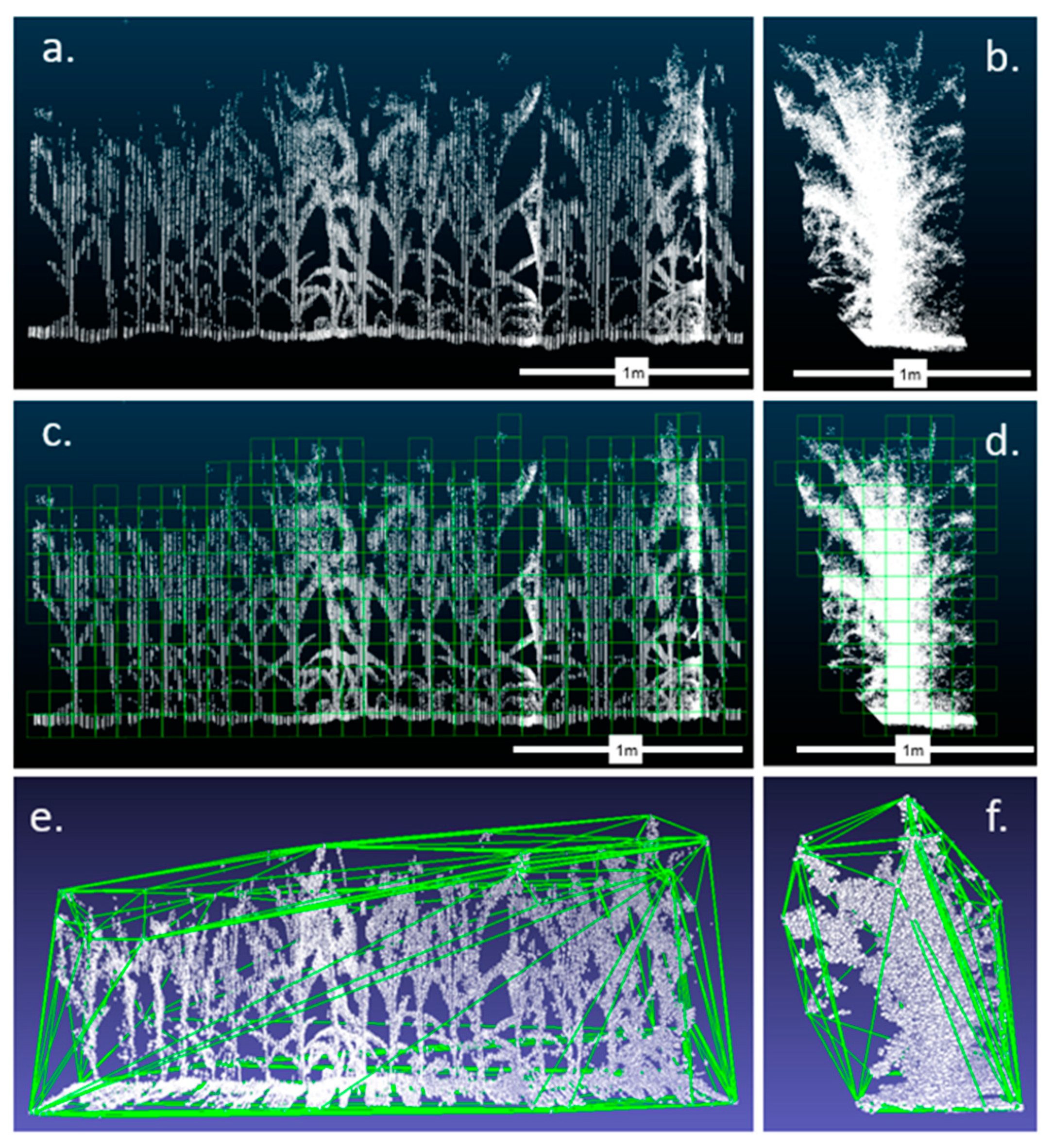
After the point cloud was processed, a voxel grid was generated from the point cloud (add_structure (“voxelgrid”) function from the Python package pyntcloud version 0.1.3). This divides the point cloud into regular cubes, similar to pixels in an image (see Figure 3c, showing voxels that are populated by points). As an example, for a 10 cm voxel grid, the first cell would contain from 0 to 10 cm (inclusive on the left bound and exclusive on the right bound) for each of the x, y, and z axes. The second cell would contain from 10 to 20 cm for the x axis and 0 to 10 cm for the y and z axes, and continued in the same manner for the other cells. Further explanation of the voxelization process with visuals can be found in the pyntcloud documentation [42]. The optimal voxel size was determined using the staggered planting experiment data, where the point cloud was analyzed using voxels with side lengths of 5 cm, 7.5 cm, 10 cm, and 15 cm. The 10 cm side length voxels were used because they correlated most strongly with the staggered planting dry mass data (5 cm: r = 0.86; 7.5 cm: r = 0.88; 10 cm: r = 0.92; 15 cm: r = 0.85). The voxel count was calculated as the number of voxels that were populated by one or more points (Figure 3c). The voxel count was divided by the ground area to produce a normalized voxel count (Figure 2). Separately, a convex hull was fit to the point cloud (‘add_structure(“convex_hull”)’ function from the Python package pyntcloud, version 0.1.3), and the volume of the convex hull was normalized to the ground area to produce a normalized volume.

2.4. Statistical Analysis of Yield Variability

Comparing the variances of two methods is a vital part of method comparison, yet variance comparisons between lidar-based biomass (m3 or voxels/m2) and destructive harvests (kg) were impossible due to unit mismatch. Therefore, the variability of hand harvests, tractor-based estimates, and lidar-based estimates of biomass were compared using the coefficient of variation (CV), calculated as
C V = S t a n d a r d   d e v i a t i o n M e a n
The standard deviation and mean have identical units, which results in the CV being dimensionless, and therefore the CVs of the different techniques can be directly compared. The CVs of biomass methods were compared using a technique from Feltz and Miller [43] (α = 0.1) that is analogous to an F-test comparison for two variances.
In the staggered planting experiment, the CV was calculated for lidar biomass and hand-harvested biomass using the three plots planted at the same time in May. In the breeding trial, the CV of lidar and harvester-based estimations of biomass was calculated using the six check lines that were replicated 16 times throughout the field. The check lines were referred to as Chk-A, Chk-B, Chk-C, Chk-D, Chk-E, and Chk-F.
Estimating CV requires repeated measurements of the same plot with each method. However, the destructive nature of harvesting makes repeated measurements impossible. However, because lidar biomass estimates were non-destructive, multiple plots of the same genotype could be measured with the lidar and sampled destructively to produce an estimate of method variance. This estimate of biomass variance was the sum of the plot-to-plot variance and the variance of the method itself.
σ b i o m a s s ,   h a r v s t e r 2 = σ p l o t t o p l o t 2 + σ h a r v e s t e r 2
σ b i o m a s s , l i d a r 2 = σ p l o t t o p l o t 2 + σ l i d a r 2
where σ b i o m a s s , h a r v e s t e r 2 and σ b i o m a s s , l i d a r 2 are the variances in biomass measurements for a set of observations from either the harvester or lidar, calculated from measuring several plots of the same genotype with a given method. σ p l o t t o p l o t 2 is the variance in biomass between plots, which is driven by varying field conditions; and σ h a r v e s t e r 2 and σ l i d a r 2 are the variances from each measurement method itself, which here are the statistics of interest.
In these two variance estimates, the contribution from σ p l o t t o p l o t 2 will be the same since both methods were used to measure the same plots. Thus, if the σ b i o m a s s , h a r v e s t e r 2 and σ b i o m a s s , l i d a r 2 differ, it will be entirely due to differences driven by σ h a r v e s t e r 2 and σ l i d a r 2 . The Feltz and Miller test was used to assess whether σ b i o m a s s , h a r v e s t e r 2 and σ b i o m a s s , l i d a r 2 were different, which can only be explained by differences in σ h a r v e s t e r 2 and σ l i d a r 2 .
It is worth noting that with this experimental design, the σ p l o t t o p l o t 2 term results in a loss of statistical power. That is, unless σ p l o t t o p l o t 2 is small or one of σ h a r v e s t e r 2 or σ l i d a r 2 is large, it is more difficult to detect a statistical difference between σ b i o m a s s , h a r v e s t e r 2 and σ b i o m a s s , l i d a r 2 .

3. Results

3.1. Convex Hull and Voxel Algorithms of Biomass Correlated Well with Hand-Harvested Biomass from the Staggered-Planting Experiment

The lidar and encoder data were combined to create 3D reconstructions of plant canopies (Figure 3a). The voxelization algorithm divides the entire point cloud into a grid of 10 cm voxels and then counts the voxels that have at least one point in them (Figure 3c). The correlation between the normalized voxel count and hand-harvested dry mass was then examined. The convex hull algorithm forms a polygon mesh around the point cloud that connects its outermost points (Figure 3e). The correlation between the normalized convex hull volume and hand-harvested dry mass was then examined.
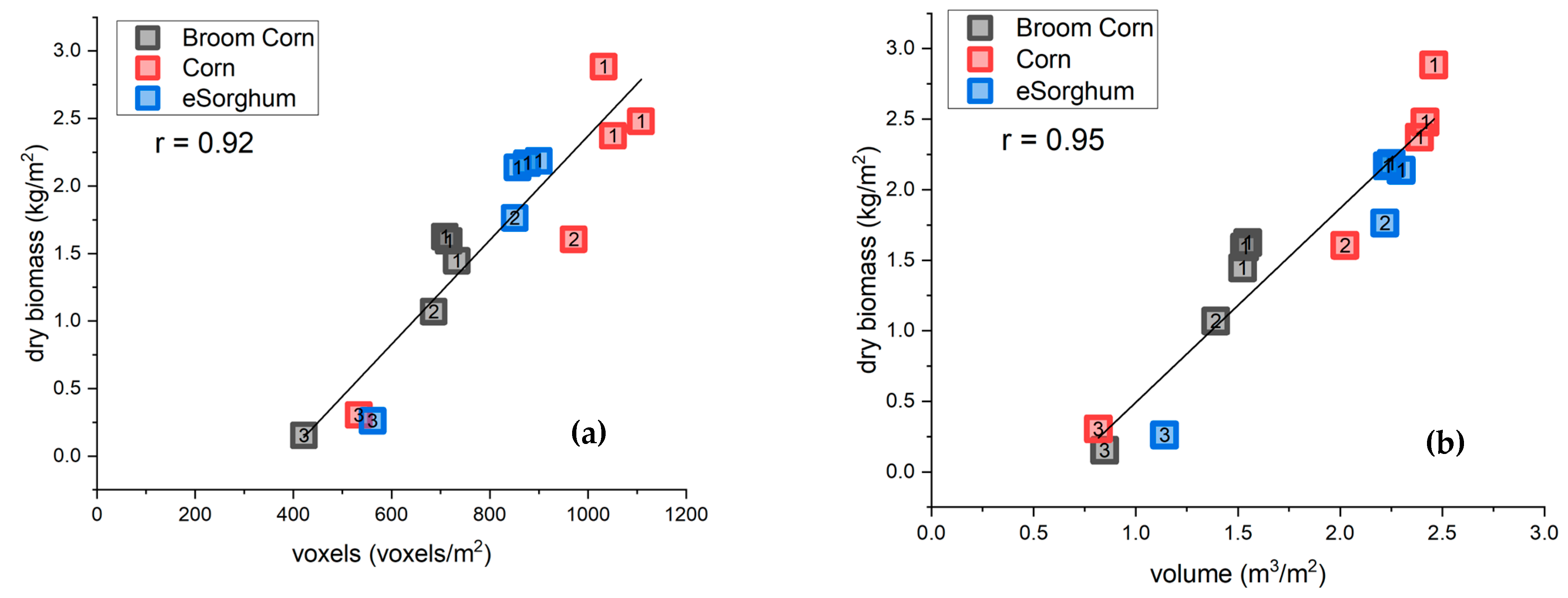
Staggered planting dates produced a wide range of biomass values, convex hull volumes, and voxel counts (Figure 4; labels 1–3). The plots from May plantings (Figure 4; label 1) have the largest biomass, June plantings (Figure 4; label 2) have intermediate biomass, and August plantings have the lowest biomass (Figure 4; label 3).
The voxel count and convex hull volumes had similar correlations (0.92 and 0.95; Figure 4) with biomass. However, correlations with corn were notably poor in that voxel count and volume estimates for the intermediate and early planting dates were similar, despite an approximately 1.5 kg m−2 difference in dry biomass. For example, there was a 5% difference in voxel count between the first and second corn plantings despite a 75% increase in biomass (Figure 4a, red labels 1 and 2).
The three replicated May plantings of each species were used to calculate the CV of biomass estimations. CVs of hand-harvested yield estimates were roughly four to seven times larger than the voxel count and convex hull estimates of biomass in broom corn and maize. Although it was not statistically significant, hand-harvest biomass CVs were smaller than lidar estimates of biomass in energy sorghum (Table 1). CVs of hand-harvested biomass estimates were larger than those of voxel count for maize and broom corn and smaller than those of voxel count in energy sorghum, but the difference was only significant in the maize measurements.

3.2. Substantial Variation of Automated Harvester Biomass Measurements Led to Poor Correlations with Digital Biomass in the Sorghum Breeding Trial

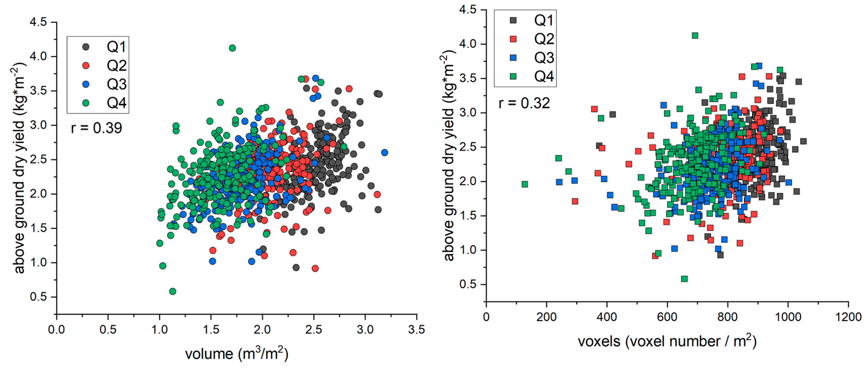
In contrast with results from the staggered planting date experiment, neither the voxel count nor the convex hull volume correlated well with harvester-based estimates of biomass from the energy sorghum breeding trial (r of 0.32 and 0.39, respectively; Figure 5). Compared to the staggered planting experiment, it is unclear if the lower correlation between destructive and digital biomass estimates in the breeding trial is driven by the lidar or mechanical harvester, or a combination of both. To assess the source of variability, we compared the CV in biomass estimates from the six replicated check lines planted throughout the field. The CVs of the harvester were 1.1 to 2.4 times larger than the CV of the convex hull volume estimate (Figure 6). The harvester CV was statistically larger than the convex hull CV in 4 out of 6 check lines (Figure 6). Similarly, the CVs of the harvester were 1.8 to 4.1 times larger than those of the voxel count. In every check line, the harvester was significantly more variable than voxel counts (Figure 6).
Comparing the CV of a method between the staggered planting experiment and the breeding trial can demonstrate if one experiment has relatively greater plot-to-plot variability ( σ p l o t t o p l o t 2 ). In the breeding trial, CVs of convex hull volume were 3 to 12 times larger, and those of voxel count were 1.5 to 6 times larger than in the staggered planting experiment (Table 1 compared to Figure 6). Biomass in the staggered planting experiment was collected by hand harvesting and drying the tissue, whereas in the breeding trial it was collected with a forage harvester that measured wet mass and corrected for water content using NIR analysis. Although plot-to-plot variability appears to be greater in the breeding trial, it is still informative to compare the CVs of the harvester and hand harvesting. The CVs from the harvester were 9 to 18 times larger than hand harvests in the staggered planting experiment (Table 1 compared to Figure 6). The fact that harvester is more variable between experiments suggests that harvester was a significant source of variation in addition to the plot-to-plot variability of the breeding trial.

4. Discussion

These experiments demonstrated the necessity of statistically comparing variances. Lidar-based biomass estimates in the staggered planting experiment displayed an excellent correlation between the hand-harvested estimations of biomass over a range of values. Convex hull volumes and voxel counts had correlation coefficients over 0.9 (Figure 4).
In the breeding trial, lidar biomass estimations correlated poorly with the harvester (r < 0.4). However, this is not an appropriate statistic to assess method quality, and further examination comparing the variances of the two instruments demonstrated that the poor correlation was due to larger variability from the harvester, not a problem with lidar biomass estimations. Compared to the staggered plot experiment, the size of the breeding experiment introduced greater plot-to-plot variability, but the harvester also had considerably larger variance than hand harvest measurements. This explains why the correlation coefficient was much lower in the breeding trial and further demonstrates how a lower correlation coefficient can have nothing to do with testing method quality. The harvester was far more variable than hand harvesting, and the plots were more variable.
Despite the challenges of using digital biomass estimates as proxies for harvested estimates, the mobile lidar platform substantially improved measurement throughput while allowing for on-site, rapid analysis. The measurements of the 960 plots of energy sorghum took three hours and forty minutes. Data storage required the push of a button to start and stop data collection for each plot. The lidar and encoder data sets were 1.1 GB for the entire breeding trial and required slightly over one hour for analysis on a consumer-grade laptop. The analysis generated a spreadsheet with all relevant phenotypes analyzed and stored the 3D point cloud data. The lidar measurement system could be modified in the future to equip newer, more powerful multi-band lidars, which would produce more points in the upper portions of the canopy and lead to better-fitting convex hull volume and voxel count measurements.
The utility of convex hull volume and voxel count as digital biomass estimates is underscored through two experiments that compared high-throughput techniques against current “gold-standard” destructive harvests. The digital estimates of biomass correlated well with hand-harvested dry weights of three different species across three different growth stages (Figure 4, Table 1). Moreover, the precision of lidar estimates of biomass relative to the harvester in the breeding trial demonstrates their potential to deliver more consistent results at scale (Figure 6). However, lidar-derived biomass still needs to be used with caution. For crops like maize, the correlation between volume and biomass can be misleading due to the disproportionate mass of reproductive tissues. This is exemplified by the minimal changes in voxel count and convex hull volume in maize pre- and post-ear growth, despite significant differences in above-ground biomass (Figure 4; red labels 1 and 2).
Reliance on r-values for method evaluation can lead to potentially misleading conclusions. For example, in the breeding trial, the low correlation for both voxel count (r = 0.32) and convex hull volume (r = 0.39) relative to the forage harvester might lead to the incorrect conclusion that digital biomass estimates are poor estimates of actual biomass (Figure 5). This assessment, however, fails to recognize crucial underlying factors behind the sources of variation that contribute to the lower correlations. The destructive biomass measurements for the replicated check lines from the forage harvester were 1.1 to 2.4 times more variable than the convex hull volume estimations and 1.8 to 4.1 times more variable than the voxel count (Figure 6). This suggests that the forage harvester was more variable than the lidar at estimating biomass and that variability was driven by the method and not plot-to-plot differences.
Since r is often useful for model development, it is mistakenly applied to method comparison studies and even used to compare results across studies. This ignores the multiple factors that affect r that make it unsuitable for method comparison within and across studies. In contrast, quantifying variances provides the advantage of facilitating cross-study experiments, as it is an inherent property of the method, provided a consistent method is used. In this study, r is presented and contrasted between the staggered planting experiment and breeding trial to demonstrate the several factors that influence the statistic and its inappropriateness for method comparison.
Overall, the goal of the statistical tests of variance is to explain why there is a lower correlation in the breeding trial than in the staggered-planting experiments. Differences in r can be caused by a different range of measured values (when there is a correlation, a wider range of values produces a larger r) or by differences in the precision of either measurement (when there is a correlation, better precision in either measurement produces a larger r) [44]. In this study, biomass values ranged from 0.25 to 3 kg m−2 in the staggered planting experiments and from 1 to 4 kg m−2 in the breeding trial (Figure 4 and Figure 5). The smaller r value and poorer correlation cannot be attributed to a smaller range, given the higher range of biomass values in the breeding trial.
The precision of the measurements was affected by the sum of two factors—plot-to-plot variance and method variance (Equations (2) and (3)). As described above, these terms cannot be separately estimated when one method is destructive, so it is not possible to formally compare values in the staggered planting and breeding trial experiments. The σ p l o t t o p l o t 2 of the breeding trial is almost certainly larger than σ p l o t t o p l o t 2 in the staggered planting experiment. The evidence that supports this is that the CVs for lidar-based estimations of biomass were consistently larger than CVs in the breeding trial. It is intuitive, too, that plots of the same genotype planted further apart would have greater σ p l o t t o p l o t 2 than plots planted close together. The plots in the staggered planting experiment were adjacent to each other, but in the breeding trial, plots were spread throughout the entire 1.1 ha field. An increase in σ p l o t t o p l o t 2 due to more variable field conditions would help explain the smaller r between the harvester and lidar measurements observed in the breeding trial. Comparing the CVs of the convex hull volume and voxel count estimates between the breeding trial and staggered planting experiments supports this, as the CVs of the convex hull volume were 3 to 12 times larger and those for the voxel count were 1.5 to 6 times larger (Table 1 compared to CVs in Figure 6).
Another factor that contributed to the poor r in the breeding trial was the relatively large   σ h a r v e s t e r 2 of the forage harvester. Biomass in the staggered planting was estimated by hand harvesting plants and drying them in an oven. In the breeding trial, biomass was estimated with a forage harvester equipped with an onboard scale and NIR moisture sensor. If σ b i o m a s s , h a r v e s t e r 2 was larger than, σ b i o m a s s , h a n d h a r v e s t 2 it would contribute to the lower r between the harvester and lidar-based estimates of biomass in the breeding trial. Indeed, the CVs of biomass estimates from the harvester were 9 to 18 times larger in the breeding trial than the CV from hand-harvesting in the staggered planting experiment (Table 1 compared to Figure 6). Thus, the greater σ p l o t t o p l o t 2 in the breeding trial compared to the staggered planting experiment (see Equation (2)) and the larger   σ h a r v e s t e r 2 of the forage harvester led to the poor relationship between digital biomass estimates and the forage harvester (Figure 5).
In other words, the correlation between the forage harvester and the lidar is poor because the plots in the breeding trial are more variable than the staggered planting and that the mechanical harvester is more variable than hand harvesting. Neither of these is related to an inherent problem with the lidar or the convex hull and the voxelization methods. These conclusions about method quality could not be determined from Figure 5 using r.
These results suggest that instrument precision should be a key consideration in method comparison and that r should not be used in method comparison studies. Rejecting a new method because it correlates poorly with the ground truth ignores the potentially significant errors of current “gold-standard” methods. Method comparison studies attempt to establish an improved quality of measurement but can be driven to incorrect conclusions when the widely used method, like the forage harvester, is assumed to be “truth”. Without quantifying variance, it may be incorrectly concluded that the lidar failed to adequately measure biomass at a larger scale, leading to the abandonment of the lidar methods, despite the lidar being more precise than the harvester.
Convex hull volume is shown as a promising algorithm for digital biomass estimation in row crops, particularly in certain species and plant developmental stages. Convex hull volume estimates appear to be an improvement in dense canopies where lidar returns may not penetrate well enough to the top of the canopy to capture structure for voxelization (Figure 3a). Furthermore, there is no need for specific parameterization. For example, multiple voxel sizes were tested to optimize the relationship between voxel count and dry biomass. However, the convex hull’s polygon mesh is formed only from the properties of the point cloud, and thus it has no parameters. A downside of the convex hull biomass estimation is that the hull around the outermost edges of the point cloud may make it insensitive to changes in plant density.
A common shortcoming of previous examinations of convex hull and voxelization algorithms is the inability to compare the quality of the new method to the established method. Although some studies reported bias [26,31], no study reported precision, failing to assess a critical parameter of method quality. For example, in a previous study, several techniques were employed to estimate tree canopy volume, and conclusions were drawn related to method consistency despite a lack of statistical precision analysis [45]. The primary difference between the methods was in the construction of the point clouds. In the study, repeated measurements of a single tree were not made, but measurements of several similar trees were. As with the checkline plots in this study, it would be possible to assess precision, but with a cost to statistical power. When doing so for the data presented in that study, the standard deviations of the two tree volume estimates were 0.24 m3 and 0.55 m3. A two-sided F-test of whether the ratio of the variances is 1 gives a p-value of 0.024, indicating that there are differences in accuracy between the two approaches employed. While this information needs to be weighed against other factors, such as cost and the need for high precision, it is itself critical information missing from that and other studies.

5. Conclusions

Lidar can significantly enhance the scale of biomass estimations with its non-destructive nature, speed, and precision. Lidar estimations of biomass were straightforward in a biomass crop like energy sorghum, but, as observed in the staggered planting experiment, challenges with machine vision remain. In this study, lidar was unable to account for the mass estimates of reproductive tissues produced from 3D point clouds. We show here that statistical tests of variance are a vital component of method comparison. Despite their strong correlation with dry weight in validation trials, lidar-based biomass estimations correlated poorly with harvester data in the larger-scale breeding trial. Without an analysis of method variance, the conclusion would have been that lidar does not work well at large scales, and digital biomass techniques would have been rejected. However, the comparison of CVs showed that the harvester was consistently more variable than the lidar, which contributed to the poor correlation between the two methods. As new phenotyping tools are being evaluated, variance analysis is an important tool to test whether legacy measurement techniques contribute disproportionately to observed variability.

Supplementary Materials

The following supporting information can be downloaded at: https://www.mdpi.com/article/10.3390/rs16122191/s1, Figure S1: A photograph of the 2019 staggered planting experiment; Figure S2: The plot design for the energy sorghum diversity panel in 2019; Figure S3 harvesting a four-row, 10ft long plot of energy sorghum from a breeding trial conducted in 2019 at the Energy Farm; Figure S4: a photo of the lidar cart being pulled through the energy sorghum breeding trial.

Author Contributions

M.H.S. contributed to conceptual development, experimental design, algorithm development, data collection, and writing the manuscript. P.F. contributed to algorithm development and writing the manuscript. B.J.B. contributed to experimental design, data collection, and writing the manuscript. S.P.L. contributed to the experimental design and writing of the manuscript. C.J.B. contributed to conceptual development, experimental design, and writing the manuscript. J.M.M. contributed to experimental design, statistical analyses, algorithm development, data collection, and writing the manuscript. All authors have read and agreed to the published version of the manuscript.

Funding

This work was funded in part by the Bill and Melinda Gates Foundation grant titled “RIPE—Realizing increased photosynthetic efficiency for sustainable increases in crop yield” (OPP1060461), the Advanced Research Projects Agency of the U.S. Department of Energy (DE-AR0000598), and the Agricultural Research Service of the United States Department of Agriculture.

Data Availability Statement

Data can be provided upon request.

Conflicts of Interest

The authors declare no competing interests.

References

  1. Atefi, A.; Ge, Y.; Pitla, S.; Schnable, J. Robotic Technologies for High-Throughput Plant Phenotyping: Contemporary Reviews and Future Perspectives. Front. Plant Sci. 2021, 12, 611940. [Google Scholar] [CrossRef] [PubMed]
  2. Herr, A.W.; Adak, A.; Carroll, M.E.; Elango, D.; Kar, S.; Li, C.; Jones, S.E.; Carter, A.H.; Murray, S.C.; Paterson, A.; et al. UAS Imagery for Phenotyping in Cotton, Maize, Soybean, and Wheat Breeding. Crop Sci. 2023, 63, 1722–1749. [Google Scholar] [CrossRef]
  3. Fu, P.; Montes, C.M.; Siebers, M.H.; Gomez-Casanovas, N.; McGrath, J.M.; Ainsworth, E.A.; Bernacchi, C.J. Advances in Field-Based High-Throughput Photosynthetic Phenotyping. J. Exp. Bot. 2022, 73, 3157–3172. [Google Scholar] [CrossRef] [PubMed]
  4. Xie, C.; Yang, C. A Review on Plant High-Throughput Phenotyping Traits Using UAV-Based Sensors. Comput. Electron. Agric. 2020, 178, 105731. [Google Scholar] [CrossRef]
  5. Meacham-Hensold, K.; Fu, P.; Wu, J.; Serbin, S.; Montes, C.M.; Ainsworth, E.; Guan, K.; Dracup, E.; Pederson, T.; Driever, S.; et al. Plot-Level Rapid Screening for Photosynthetic Parameters Using Proximal Hyperspectral Imaging. J. Exp. Bot. 2020, 71, 2312–2328. [Google Scholar] [CrossRef] [PubMed]
  6. Montes, C.M.; Fox, C.; Sanz-Sáez, Á.; Serbin, S.P.; Kumagai, E.; Krause, M.D.; Xavier, A.; Specht, J.E.; Beavis, W.D.; Bernacchi, C.J.; et al. High-Throughput Characterization, Correlation, and Mapping of Leaf Photosynthetic and Functional Traits in the Soybean (Glycine Max) Nested Association Mapping Population. Genetics 2022, 221, iyac065. [Google Scholar] [CrossRef] [PubMed]
  7. Spindel, J.E.; Dahlberg, J.; Colgan, M.; Hollingsworth, J.; Sievert, J.; Staggenborg, S.H.; Hutmacher, R.; Jansson, C.; Vogel, J.P. Association Mapping by Aerial Drone Reveals 213 Genetic Associations for Sorghum Bicolor Biomass Traits under Drought. BMC Genom. 2018, 19, 679. [Google Scholar] [CrossRef] [PubMed]
  8. Gage, J.L.; Richards, E.; Lepak, N.; Kaczmar, N. In-Field Whole-Plant Maize Architecture Characterized by Subcanopy Rovers and Latent Space Phenotyping. Plant Phenome 2019, 2, 1–11. [Google Scholar] [CrossRef]
  9. Siebers, M.H.; Edwards, E.J.; Jimenez-Berni, J.A.; Thomas, M.R.; Salim, M.; Walker, R.R. Fast Phenomics in Vineyards: Development of GRover, the Grapevine Rover, and LiDAR for Assessing Grapevine Traits in the Field. Sensors 2018, 18, 2924. [Google Scholar] [CrossRef] [PubMed]
  10. Sun, S.; Li, C.; Paterson, A.H.; Jiang, Y.; Xu, R.; Robertson, J.S.; Snider, J.L.; Chee, P.W. In-Field High Throughput Phenotyping and Cotton Plant Growth Analysis Using LiDAR. Front. Plant Sci. 2018, 9, 16. [Google Scholar] [CrossRef]
  11. Rosell Polo, J.R.; Sanz, R.; Llorens, J.; Arnó, J.; Escolà, A.; Ribes-Dasi, M.; Masip, J.; Camp, F.; Gràcia, F.; Solanelles, F.; et al. A Tractor-Mounted Scanning LIDAR for the Non-Destructive Measurement of Vegetative Volume and Surface Area of Tree-Row Plantations: A Comparison with Conventional Destructive Measurements. Biosyst. Eng. 2009, 102, 128–134. [Google Scholar] [CrossRef]
  12. Bailey, B.N.; Mahaffee, W.F. Rapid Measurement of the Three-Dimensional Distribution of Leaf Orientation and the Leaf Angle Probability Density Function Using Terrestrial LiDAR Scanning. Remote Sens. Environ. 2017, 194, 63–76. [Google Scholar] [CrossRef]
  13. Su, Y.; Wu, F.; Ao, Z.; Jin, S.; Qin, F.; Liu, B.; Pang, S.; Liu, L.; Guo, Q. Evaluating Maize Phenotype Dynamics under Drought Stress Using Terrestrial Lidar. Plant Methods 2019, 15, 11. [Google Scholar] [CrossRef] [PubMed]
  14. Vélez, S.; Ariza-Sentís, M.; Valente, J. VineLiDAR: High-Resolution UAV-LiDAR Vineyard Dataset Acquired over Two Years in Northern Spain. Data Brief 2023, 51, 109686. [Google Scholar] [CrossRef] [PubMed]
  15. Das Choudhury, S.; Maturu, S.; Samal, A.; Stoerger, V.; Awada, T. Leveraging Image Analysis to Compute 3D Plant Phenotypes Based on Voxel-Grid Plant Reconstruction. Front. Plant Sci. 2020, 11, 521431. [Google Scholar] [CrossRef] [PubMed]
  16. Greaves, H.E.; Vierling, L.A.; Eitel, J.U.H.; Boelman, N.T.; Magney, T.S.; Prager, C.M.; Griffin, K.L. Estimating Aboveground Biomass and Leaf Area of Low-Stature Arctic Shrubs with Terrestrial LiDAR. Remote Sens. Environ. 2015, 164, 26–35. [Google Scholar] [CrossRef]
  17. Jimenez-Berni, J.A.; Deery, D.M.; Rozas-Larraondo, P.; Condon, A.T.G.; Rebetzke, G.J.; James, R.A.; Bovill, W.D.; Furbank, R.T.; Sirault, X.R.R. High Throughput Determination of Plant Height, Ground Cover, and Above-Ground Biomass in Wheat with LiDAR. Front. Plant Sci. 2018, 9, 237. [Google Scholar] [CrossRef]
  18. Li, Y.; Hu, R.; Xing, Y.; Pang, Z.; Chen, Z.; Niu, H. Comparison of Three Approaches for Estimating Understory Biomass in Yanshan Mountains. Remote Sens. 2024, 16, 1060. [Google Scholar] [CrossRef]
  19. Nguyen, V.-T.; Fournier, R.A.; Côté, J.-F.; Pimont, F. Estimation of Vertical Plant Area Density from Single Return Terrestrial Laser Scanning Point Clouds Acquired in Forest Environments. Remote Sens. Environ. 2022, 279, 113115. [Google Scholar] [CrossRef]
  20. Colaço, A.F.; Schaefer, M.; Bramley, R.G.V. Broadacre Mapping of Wheat Biomass Using Ground-Based LiDAR Technology. Remote Sens. 2021, 13, 3218. [Google Scholar] [CrossRef]
  21. Rivera, G.; Porras, R.; Florencia, R.; Sánchez-Solís, J.P. LiDAR Applications in Precision Agriculture for Cultivating Crops: A Review of Recent Advances. Comput. Electron. Agric. 2023, 207, 107737. [Google Scholar] [CrossRef]
  22. Béland, M.; Baldocchi, D.D.; Widlowski, J.-L.; Fournier, R.A.; Verstraete, M.M. On Seeing the Wood from the Leaves and the Role of Voxel Size in Determining Leaf Area Distribution of Forests with Terrestrial LiDAR. Agric. For. Meteorol. 2014, 184, 82–97. [Google Scholar] [CrossRef]
  23. Preparata, F.P.; Shamos, M.I. Computational Geometry: An Introduction (Texts and Monographs in Computer Science), 1st ed.; Springer: Berlin/Heidelberg, Germany, 1985; ISBN 9780387961316. [Google Scholar]
  24. Yan, Z.; Liu, R.; Cheng, L.; Zhou, X.; Ruan, X.; Xiao, Y. A Concave Hull Methodology for Calculating the Crown Volume of Individual Trees Based on Vehicle-Borne LiDAR Data. Remote Sens. 2019, 11, 623. [Google Scholar] [CrossRef]
  25. Wu, B.; Yu, B.; Yue, W.; Shu, S.; Tan, W.; Hu, C.; Huang, Y.; Wu, J.; Liu, H. A Voxel-Based Method for Automated Identification and Morphological Parameters Estimation of Individual Street Trees from Mobile Laser Scanning Data. Remote Sens. 2013, 5, 584–611. [Google Scholar] [CrossRef]
  26. Korhonen, L.; Vauhkonen, J.; Virolainen, A.; Hovi, A.; Korpela, I. Estimation of Tree Crown Volume from Airborne Lidar Data Using Computational Geometry. Int. J. Remote Sens. 2013, 34, 7236–7248. [Google Scholar] [CrossRef]
  27. Zhou, L.; Li, X.; Zhang, B.; Xuan, J.; Gong, Y.; Tan, C.; Huang, H.; Du, H. Estimating 3D Green Volume and Aboveground Biomass of Urban Forest Trees by UAV-Lidar. Remote Sens. 2022, 14, 5211. [Google Scholar] [CrossRef]
  28. Tao, S.; Guo, Q.; Li, L.; Xue, B.; Kelly, M.; Li, W.; Xu, G.; Su, Y. Airborne Lidar-Derived Volume Metrics for Aboveground Biomass Estimation: A Comparative Assessment for Conifer Stands. Agric. For. Meteorol. 2014, 198–199, 24–32. [Google Scholar] [CrossRef]
  29. Fernández-Sarría, A.; López-Cortés, I.; Estornell, J.; Velázquez-Martí, B.; Salazar, D. Estimating Residual Biomass of Olive Tree Crops Using Terrestrial Laser Scanning. Int. J. Appl. Earth Obs. Geoinf. 2019, 75, 163–170. [Google Scholar] [CrossRef]
  30. Altman, D.G.; Bland, J.M. Measurement in Medicine: The Analysis of Method Comparison Studies. J. R. Stat. Society. Ser. D Stat. 1983, 32, 307–317. [Google Scholar] [CrossRef]
  31. Stovall, A.E.L.; Vorster, A.G.; Anderson, R.S.; Evangelista, P.H.; Shugart, H.H. Non-Destructive Aboveground Biomass Estimation of Coniferous Trees Using Terrestrial LiDAR. Remote Sens. Environ. 2017, 200, 31–42. [Google Scholar] [CrossRef]
  32. Putman, E.B.; Popescu, S.C. Automated Estimation of Standing Dead Tree Volume Using Voxelized Terrestrial Lidar Data. IEEE Trans. Geosci. Remote Sens. 2018, 56, 6484–6503. [Google Scholar] [CrossRef]
  33. Lin, C.; Hu, F.; Peng, J.; Wang, J.; Zhai, R. Segmentation and Stratification Methods of Field Maize Terrestrial LiDAR Point Cloud. Collect. FAO Agric. 2022, 12, 1450. [Google Scholar] [CrossRef]
  34. Thapa, S.; Zhu, F.; Walia, H.; Yu, H.; Ge, Y. A Novel LiDAR-Based Instrument for High-Throughput, 3D Measurement of Morphological Traits in Maize and Sorghum. Sensors 2018, 18, 1187. [Google Scholar] [CrossRef] [PubMed]
  35. Ott, L.R.; Longnecker, M.T. An Introduction to Statistical Methods and Data Analysis, 7th ed.; Cengage Learning: Boston, MA, USA, 2015; ISBN 9781305269477. [Google Scholar]
  36. Yen, J.; Leber, D.; Pibida, L. Comparing Instruments; National Institute of Standards and Technology: Gaithersburg, MA, USA, 2020.
  37. McGrath, J.M.; Siebers, M.H.; Fu, P.; Long, S.P.; Bernacchi, C.J. To Have Value, Comparisons of High-Throughput Phenotyping Methods Need Statistical Tests of Bias and Variance. Front. Plant Sci. 2023, 14, 1325221. [Google Scholar] [CrossRef] [PubMed]
  38. Ferguson, J.N.; Fernandes, S.B.; Monier, B.; Miller, N.D.; Allen, D.; Dmitrieva, A.; Schmuker, P.; Lozano, R.; Valluru, R.; Buckler, E.S.; et al. Machine Learning-Enabled Phenotyping for GWAS and TWAS of WUE Traits in 869 Field-Grown Sorghum Accessions. Plant Physiol. 2021, 187, 1481–1500. [Google Scholar] [CrossRef] [PubMed]
  39. Institute for Sustainability, Energy, and Environment at the University of Illinois Energy Farm Sorghum Harvest Part Two. Available online: https://www.youtube.com/watch?v=rS9fR-_u-uY (accessed on 15 April 2024).
  40. Grubbs, F.E. Sample Criteria for Testing Outlying Observations. Ann. Math. Stat. 1950, 21, 27–58. [Google Scholar] [CrossRef]
  41. de la Iglesia Castro, D. Pyntcloud: Pyntcloud Is a Python Library for Working with 3D Point Clouds; Github: San Francisco, CA, USA, 2023. [Google Scholar]
  42. de la Iglesia Castro, D. Examples/[Structures] VoxelGrid.ipynb at Master Daavoo/Pyntcloud; Github: San Francisco, CA, USA, 2018. [Google Scholar]
  43. Feltz, C.J.; Miller, G.E. An Asymptotic Test for the Equality of Coefficients of Variation from K Populations. Stat. Med. 1996, 15, 646–658. [Google Scholar] [CrossRef]
  44. Goodwin, L.D.; Leech, N.L. Understanding Correlation: Factors That Affect the Size of R. J. Exp. Educ. 2006, 74, 251–266. [Google Scholar] [CrossRef]
  45. Auat Cheein, F.A.; Guivant, J. SLAM-Based Incremental Convex Hull Processing Approach for Treetop Volume Estimation. Comput. Electron. Agric. 2014, 102, 19–30. [Google Scholar] [CrossRef]
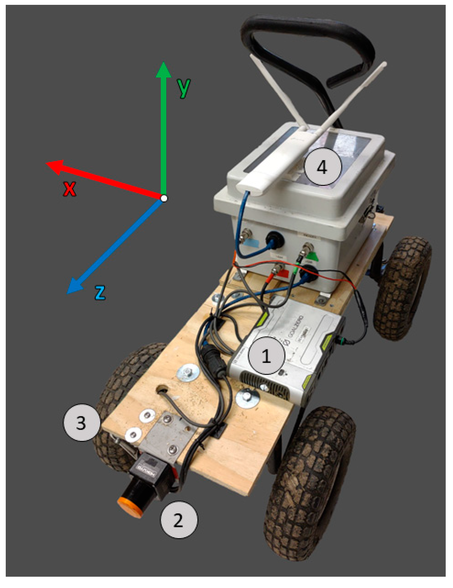
Figure 1. (1) The instruments were powered by a 12 V lithium-ion battery. (2) A 2D scanning lidar (Hokuyo LX10, Hokuyo Automatic, Osaka, Japan) was mounted to the cart 9 inches above the ground. (3) The distance the system traveled was measured using a rotary encoder (Yumo E6B2-CWZ3E, Yumo Automation, Yueqing, China) connected to the wheel with a belt. (4) Data were transmitted via a wireless access point (TP-link, EAP110 outdoor access point, Irving, CA, USA) and stored on a laptop. The lidar scans were made in the x and y coordinates. The z coordinate was the distance traveled by the system, measured by the encoder.
Remotesensing 16 02191 g001
Figure 2. Flow chart of data analysis, from data collection to traits of interest, with arrows between boxes that explain the steps. Red boxes are the data collected by the lidar system. Tan boxes represent data produced during processing steps. The green boxes are the digital biomass estimates.
Remotesensing 16 02191 g002
Figure 3. A representative scan of a maize plot visualized along the x axis (a,c,e) and along the z axis (b,d,f) from the shortest plot of the last staggered planting date when plants were ~1 m tall. A visualization of the voxelization algorithm (c,d) shows only the grid cells (voxels) that contain points. The number of occupied voxels was counted for the analysis. Panels (e,f) show a visualization of the convex hull algorithm, where the outermost points of the point cloud are connected to form a polygon mesh around the point cloud. Panels (ad) were visualized using CloudCompare (https://www.danielgm.net/cc/, accessed on 15 June 2024). Panels (e,f) were visualized using MeshLab (accessed on 15 June 2024).
Remotesensing 16 02191 g003
Figure 4. The relationship between plant biomass (kg m−2), including reproductive tissues, and the lidar based estimation of biomass: (a) voxel-based estimation of biomass (voxels m−2); voxels had 10 cm side lengths. (b) and convex-hull-based estimations of volume. The measurements were made on broom corn, corn, and energy sorghum plots in the staggered planting date experiment. The color of the symbol corresponds to the species. The number inside each symbol indicates the planting date. In May (label 1), three plots of each species were planted to give repeated end-of-season destructive estimates. The three species were planted again in June (label 2) and July (label 3) to give a chronoseries of plant growth stages in a small area.
Remotesensing 16 02191 g004
Figure 5. Scatterplots of biomass estimated from the harvester versus either area-adjusted voxel (left) or convex-hull estimations of volume (right). Energy sorghum varieties in this trial were planted in four quadrants based on height to avoid the taller genotypes shading the shorter ones (Supplemental Figure S2, the quadrants there are labeled as “sets”). Q1 contained the tallest varieties, and Q4 contained the shortest varieties.
Remotesensing 16 02191 g005
Figure 6. Normalized measurements from each of the three methods in the breeding trial. Biomass was estimated as a plot-adjusted volume with the lidar and measured destructively by the harvester. Since the values are normalized, the height of each bar (from the lower error bar to the upper error bar) is a visual representation of the CV. Six check lines (CHK-A… F) were replicated 16 times throughout the breeding trial. The relative yield ([biomass observation]/[mean of the method for that checkline]) is plotted for each of the 16 replicates of each checkline and method. The CV of each method is included in a table below each set of box plots. The CVs of the lidar-based biomass (convex hull volume and voxel count) estimates were compared to the CV of the harvester estimates after Feltz and Miller 1996. An asterisk above a box plot denotes that the CV, or spread of the data, is different between the lidar method and harvester (p ≤ 0.1).
Remotesensing 16 02191 g006
Table 1. The coefficient of variation (CV) of three biomass estimations made on three species. Biomass was estimated as plot-adjusted volume with the lidar and measured destructively by hand harvesting 2 m of plant material, drying it, and weighing it. A larger CV value indicates greater variability.
SpeciesConvex Hull VolumeVoxelHand-Harvested Dry MassHand Harvest/VolumeHand Harvest/Voxel
Broom Corn0.0080.0170.0627.367 *3.598
Energy Sorghum0.0150.0370.0110.7780.308
Maize0.0150.0240.1056.854 *4.258 *
* significant difference between the hand harvest and digital biomass (p < 0.1).
Disclaimer/Publisher’s Note: The statements, opinions and data contained in all publications are solely those of the individual author(s) and contributor(s) and not of MDPI and/or the editor(s). MDPI and/or the editor(s) disclaim responsibility for any injury to people or property resulting from any ideas, methods, instructions or products referred to in the content.