Abstract
Leaf chlorophyll content (LCC) is an important indicator of plant nutritional status and can be a guide for plant disease diagnosis. In this study, we took apple leaves infected with mosaic disease as a research object and extracted two types of information on spectral and textural features from hyperspectral images, with a view to realizing non-destructive detection of LCC. First, the collected hyperspectral images were preprocessed and spectral reflectance was extracted in the region of interest. Subsequently, we used the successive projections algorithm (SPA) to select the optimal wavelengths (OWs) and extracted eight basic textural features using the gray-level co-occurrence matrix (GLCM). In addition, composite spectral and textural metrics, including vegetation indices (VIs), normalized difference texture indices (NDTIs), difference texture indices (DTIs), and ratio texture indices (RTIs) were calculated. Third, we applied the maximal information coefficient (MIC) algorithm to select significant VIs and basic textures, as well as the tandem method was used to fuse the spectral and textural features. Finally, we employ support vector regression (SVR), backpropagation neural network (BPNN), and K-nearest neighbors regression (KNNR) methods to explore the efficacy of single and combined feature models for estimating LCC. The results showed that the VIs model (R2 = 0.8532, RMSE = 2.1444, RPD = 2.6179) and the NDTIs model (R2 = 0.7927, RMSE = 2.7453, RPD = 2.2032) achieved the best results among the single feature models for spectra and texture, respectively. However, textural features generally exhibit inferior regression performance compared to spectral features and are unsuitable for standalone applications. Combining textural and spectral information can potentially improve the single feature models. Specifically, when combining NDTIs with VIs as input parameters, three machine learning models outperform the best single feature model. Ultimately, SVR achieves the highest performance among the LCC regression models (R2 = 0.8665, RMSE = 1.8871, RPD = 2.7454). This study reveals that combining textural and spectral information improves the quantitative detection of LCC in apple leaves infected with mosaic disease, leading to higher estimation accuracy.
1. Introduction
Apples are one of the most important economic crops cultivated globally, and these fruit trees’ healthy growth is significant for economic development and environmental protection. Apple mosaic disease, caused by the apple mosaic virus, is a prevalent viral disease in the management of apple cultivation. Improper control will affect the ability of leaf photosynthesis to make nutrients and seriously affect the quality of fruit and yield [1]. The primary symptoms of apple mosaic disease are observed in the leaves; depending on the severity of the infection, the physiological properties of the leaves change, manifesting as variegation, mottling, and necrosis, typically characterized by chlorosis. Chlorophyll is a critical pigment in photosynthesis directly involved in capturing and converting light energy. Leaf chlorophyll content (LCC) serves as an excellent indicator of photosynthetic activity, mutations, stress, and nutritional status [2] and holds particular significance for precision agriculture. Studies have shown that LCC can reflect the plant’s health status and response to external environmental stresses [3,4]. Therefore, measuring LCC can provide a timely and accurate assessment of the plant’s physiological condition, offering a scientific basis for the early diagnosis and control of diseases. At the same time, the spatial distribution of leaf pigments also serves as an essential indicator of pest and disease stress [5].
Traditional methods for detecting LCC involve grinding plant tissues to extract target compounds for quantification using various chemical methods. Although these methods are reproducible and accurate, they are time-consuming and labor-intensive. The irreversible damage to the samples and the delay in time restrict further analysis, failing to meet the needs for timely and effective disease monitoring. The development of optical sensors and computer-assisted technologies has provided a high-precision pathway for detection [6,7,8]. Hyperspectral imaging (HSI), as an emerging sensor technology, has been widely applied to the non-destructive monitoring of internal components of plants. HSI can acquire a three-dimensional data cube containing spatial information by integrating machine vision with spectroscopic techniques. The first two dimensions provide spatial details, while the third offers spectral information across hundreds of continuous wavelengths [9]. This technology not only measures the plants’ absorption and reflection characteristics across different wavelengths but also captures the minute textural and structural features, allowing for an intuitive recognition and diagnosis of plant health.
Currently, numerous domestic and international scholars are employing HSI to delve into the physiological and biochemical information within various crops. Spectral methods are the most commonly used techniques, with critical solutions focusing on extracting features sensitive to biochemical parameters [10,11]. For instance, Li et al. [12] compared various feature selection algorithms, such as the successive projections algorithm (SPA), random frog (RF), and competitive adaptive reweighted sampling (CARS), to identify wavelengths with optimal sensitivity and applied them in studying the LCC distribution in lemon leaves infected with the CYVCV virus. Gai et al. [13] accurately estimated the LCC in sugarcane leaves using features extracted by SPA combined with a stacking regression model, achieving recognition accuracies as high as 98.34%. Compared to models based on specific spectral bands, spectral indices have the advantage of enhancing spectral features according to the research objectives, thereby amplifying the correlation between spectral reflectance and crop biochemical information and reducing the sensitivity of single bands to other influencing factors [14,15,16]. Extensive research has focused on developing spectral indices models to estimate the LCC in crop leaves, showing promising application potential [2,17,18,19,20,21]. These studies indicate that the spectral information in hyperspectral images performs well in detecting the internal characteristics of crops. However, most studies have not considered the correlation between the two-dimensional spatial information in hyperspectral images and crop health status. Infected plants exhibit changes in external features, and textural information can quantify attributes of crop phenotypic structure and tissue arrangement, thus extracting more potential information from images [22,23]. In recent years, some studies have applied textural features in researching plant biochemical states, affirming the capability of combining spectral and image information to estimate plant physiological parameters [24,25]. Xie et al. [26] used spectral and textural information from hyperspectral images to build a detection model for tomato early blight disease, proving that models based on spectral features outperform those based on textural features, using spectral reflectance achieving a 100% recognition rate. Yan et al. [27] compared single and fused models based on spectral data and image texture data in studying pothos leaves, finding that the fusion method yielded the best prediction results. Sun et al. [24] extracted textural information from principal component images and characteristic wavelength images, using fusion methods of spectral and textural information to detect nitrogen in lettuce leaves, finding that the model based on spectral data combined texture data from four characteristic wavelength images performed best from the calibration performance index.
The above research demonstrates that combining spectral and textural features to improve the accuracy of estimating crop biochemical status has promising prospects. However, studies on apple leaves infected with mosaic disease are rare, and most research focuses on solving classification problems, including distinguishing between healthy and diseased leaves and assessing the severity of diseases, with limited research on using regression algorithms to quantitatively invert biochemical parameters. Therefore, this study aims to: (1) analyze the spectral and textural features of apple leaves infected with mosaic disease; (2) construct and select the spectral and textural parameters of LCC estimation models; (3) assess the model performance of the single and combined features of spectral and textural information; (4) determine the optimal combination of spectral and textural features for estimating LCC, to establish a non-destructive hyperspectral model for estimating LCC in apple leaves.
2. Materials and Methods
2.1. Experimental Design
The experiment was conducted at an orchard in Wuquan Town, Yangling District, Xianyang City, Shaanxi Province (Figure 1). The leaf collection time was selected at the peak of the mosaic disease (26 April 2023), when the disease was developing rapidly and the symptoms were obvious. Healthy apple leaves and leaves with different degrees of mosaic disease were collected in separate bags, put into an insulated box with built-in ice packs, and returned to the laboratory for indoor data collection after a quick sorting. In order to ensure a balanced sample, the leaves were classified into four grades according to the degree of variability of leaf spots and the percentage of spot area compared to the whole leaf area (Table 1).
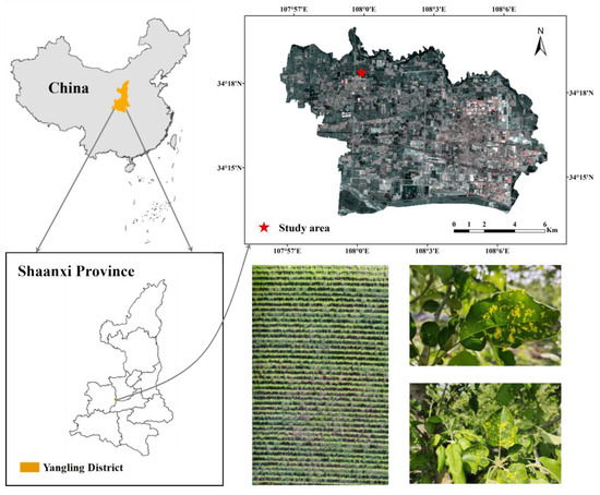
Figure 1.
Location of the experimental area and pictures of the experiments.

Table 1.
Criteria for grading the degree of leaf disease.
2.2. LCC Determination
The Dualex Scientific+ (FORCE-A, Orsay, France) was utilized to measure the LCC in apple leaves and provide non-destructive, real-time assessments. The analyzer is factory-calibrated to record LCC in μg/cm2 [28,29]. Four randomly chosen locations on each leaf were sampled, excluding the midvein and leaf edges. Each measurement was conducted thrice, and the mean value was considered the LCC at that particular point.
2.3. Hyperspectral Image Collection and Processing
2.3.1. Hyperspectral Image Acquisition and Calibration
Hyperspectral image acquisition is conducted using a hyperspectral imaging system comprising five components: a hyperspectral imager, two halogen lamps, a tripod, a standard gray panel, and a low-reflectivity black cotton cloth, as shown in Figure 2. This experiment used the SOC 710VP portable hyperspectral imager (Surface Optics Corp, San Diego, CA, USA), equipped with a 12 mm Schneider Xenoplan™ lens. Its internal scanning mechanism swiftly acquires grayscale images across 128 bands, spanning from 374.81 to 1042.15 nm, thereby creating a hyperspectral data block. The sensor system boasts a spectral resolution of 4.6875 nm and an image resolution of 696 × 520 pixels. In the darkroom, two halogen lamps were utilized to simulate natural light conditions, the leaves were placed horizontally on a black cotton cloth alongside a standard gray panel, and the camera was aligned vertically downward on the black cloth. Adjust the camera focus by turning the focus wheel on the lens until the samples are clear in the focus window. Place the camera’s lens cover on to capture dark noise data, then remove the cover to acquire images of the leaf sample and gray panel. Black and white plate correction of hyperspectral images is necessary due to variations in the intensity of the light source across each band of the image and interference from instrumental and environmental noise:
where is the corrected hyperspectral image, is the original hyperspectral image, is the dark current image, and is the reference plate image.
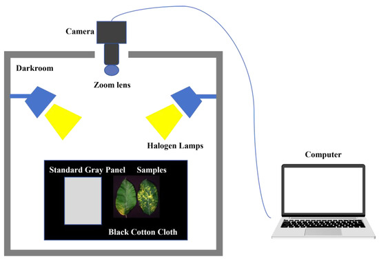
Figure 2.
Hyperspectral imaging system.
2.3.2. Image Segmentation and Selection of Region of Interest (ROI)
To focus on the spectral or textural features of the blade itself and eliminate the interfering information from the image background, we have taken a series of image processing. Using a hyperspectral image of a single leaf as a case study, we initially applied the PPR (Plant Pigment Ratio) vegetation indicated in Equation (2) to assess the significant contrast between the leaf and its background. Figure 3 indicates the maximum reflectance difference between background and leaf pixels occurs in the visible spectra (400–760 nm). The spectral variation in the black cloth and shadow is relatively stable, whereas the spectral changes in healthy or infected leaves are significant, particularly in the green peak region around 550 nm. Leaves absorb the blue band and reflect the green band; PPR employs normalization operations to enhance the contrast in reflectance between the background and the leaves.
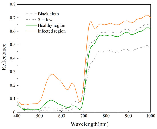
Figure 3.
Spectral curves of apple leaves and background.
Subsequently, the original image in Figure 4a underwent PPR exponential processing, resulting in a grayscale map with an easily adjustable threshold value, as depicted in Figure 4b. Following this, a binarization step was executed on the grayscale map, with a threshold value of 0.28 selected to designate pixel points corresponding to the leaf and background as 1 and 0 (Figure 4c). The resultant mask was applied to the original spectral image (Figure 4d), effectively isolating the leaf information while ensuring analytical accuracy and efficiency. Using the region of interest (ROI) tool in ENVI 5.3 (Exelis, McLean, VA, USA), a 25 × 25 pixel matrix was manually selected corresponding to the LCC measurement points of the blades, leaving four ROIs per blade for the extraction of spectral and textural features of the image.
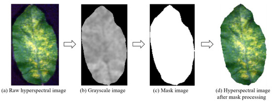
Figure 4.
Hyperspectral image segmentation.
2.4. Data Processing
This study established LCC detection models for apple leaves infected mosaic disease based on HSI, combined with spectral and textural information. Figure 5 illustrates the flowchart. First, the hyperspectral images of the apple leaves were collected and processed. Next, we extracted spectral features and textural features, including six indicators. Third, we established single and combined prediction models of LCC based on three machine learning algorithms. Finally, we mapped the LCC distribution using the best spectral, textural, and combined spectra-texture feature model.
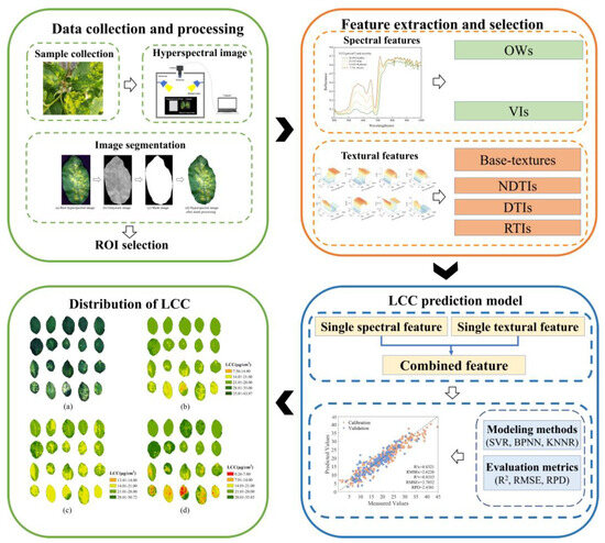
Figure 5.
Flowchart of data analysis and processing.
2.4.1. Extraction of Spectral Data and Selection of Optimal Wavelengths
In order to obtain more accurate spectral features, we excluded bands with low signal-to-noise ratios from both ends of the original spectral data. We focused on wavelengths ranging from 400 to 1000 nm. For each wavelength, we calculated the average spectral reflectance value of all pixels within the selected ROIs, resulting in 480 spectral samples. The acquisition of raw spectra data by the imaging spectrometer is susceptible to influences from the instrument and background noise in the experimental environment. To mitigate these interferences, preprocessing is essential to extract information pertinent to the samples [30,31]. In this study, we employed the Savitzky–Golay (SG) method to eliminate extraneous noise factors effectively, facilitating subsequent analysis and model construction.
Even after noise reduction, the spectral data still present a significant issue of redundancy, which hinders the investigation into the response mechanism between LCC and spectral data. Therefore, it is imperative to identify and select effective wavelengths closely correlated with LCC. This will streamline the model’s complexity and enhance computational efficiency, as discussed in the literature [32,33]. In this study, the SPA is employed to identify optimal wavelengths (OWs). SPA is a forward variable selection technique that starts with a single wavelength. With each iteration, an additional wavelength is incorporated until a specified number of wavelengths, N, is reached [34]. The core procedure involves initially choosing a wavelength at random and then calculating its projection onto the set of unselected wavelengths. The wavelength that exhibits the largest projection vector is then incorporated into the selected wavelength sequence. This operation is performed N times, ensuring that with each iteration, the selected wavelengths exhibit minimal linear redundancy compared to the previously chosen wavelengths. Ultimately, this method yields a subset of wavelengths with the full-wavelength spectral dataset [35]. Throughout the process, the selection is guided by root mean square error (RMSE) and the F-test with an alpha level of 0.25. The ultimate selection points determined by the F-test have no significant deviation from the minimum RMSE value, ensuring that the model’s efficacy is preserved while minimizing the feature set as much as possible. We implemented the SG and SPA algorithms in MATLAB R2021b.
2.4.2. Sample Split
In the quantitative diagnosis of LCC, the sample set partitioning method affects the modeling accuracy and stability of the model [36]. SPXY (sample set partitioning based on joint x-y distances) considers the spatial variability in both x and y dimensions when calculating the inter-sample distances. Compared to partitioning schemes based on x information alone or random sampling, this approach can more efficiently cover the multidimensional vector space. It ensures that the distributional characteristics of the samples are more comprehensively and accurately captured, thereby increasing the diversity and representativeness among the samples [37,38]. The samples were divided at a ratio of 2:1, resulting in 320 samples for the calibration set and 160 samples for the validation set. Table 2 shows the statistical information dataset split using the SPXY algorithm.

Table 2.
The statistical information of the sample set.
2.4.3. Vegetation Indices Extraction
Numerous scholars have analyzed the spectral information of plants to identify the characteristic absorption bands for chlorophyll content. They have developed indices for estimating chlorophyll content by utilizing spectral reflectance and derivative spectra, along with various derived combinations of these spectra. This study computes thirty commonly used chlorophyll-sensitive spectral indices within the 400–1000 nm wavelength range, as listed in Table 3.

Table 3.
Empirical vegetation indices and calculation formulas.
2.4.4. Image Textural Feature Extraction and Texture Indices Construction
This study utilizes the gray-level co-occurrence matrix (GLCM), a prevalent method for delineating image textures, to extract texture metrics from defined ROIs. GLCM quantifies the co-occurrence frequency of pixel intensity values at specified directions and distances, thereby revealing the spatial correlation characteristics of image gray levels [61,62]. Although the GLCM provides comprehensive information regarding grayscale directionality, adjacency, and the amplitude of variations, it does not directly yield features discriminative enough for texture differentiation. Consequently, this study leverages the data obtained from GLCM to describe eight basic textural features, as detailed in Table 4. For each hyperspectral sample, textural features are computed at 0°, 45°, 90°, and 135° orientations within a 3 × 3 GLCM window, assigning values to the central pixel with a set gray level of 16 and a distance of 1. Wavelengths isolated through feature selection are identified as potential indicators for predicting LCC [63,64,65]. Consequently, basic textural features are extracted from the grayscale images corresponding to these optimum wavelengths.

Table 4.
The gray-level co-occurrence matrix (GLCM) textural features used in this study.
Furthermore, to elucidate the synergistic effects of two types of texture features on LCC, normalized difference texture index (NDTI), difference texture index (DTI), and ratio texture index (RTI) for pairwise texture features (T1, T2) are computed as Equations (3)–(5) [66,67,68]. These textural features are calculated in Python 3.9.
2.4.5. Vegetation Indices and Textural Features Selection
For a set of initial trait variables, selecting an informative and representative subset can improve the quality of description and effectiveness in detecting crop traits. Spectral and textural data typically possess complex structures and properties, which may prevent linear methods from adequately capturing the relationships between them, thereby limiting the sensitivity of the analysis. The maximal information coefficient (MIC), proposed by Reshef et al. [69], is a resilient method for assessing the correlation between variables based on characteristics of their probability distributions. It measures the strength of linear and nonlinear relationships between two variables, X and Y, and is recognized for its broad applicability and high robustness as a filtering algorithm. MIC enhances the mutual information framework by integrating the concepts of grids and normalization to facilitate the discretization and analysis of metrics. Mutual information measures the amount of information one random variable holds about another and is mathematically defined as follows:
where is the joint probability density of x and y, and are the marginal probability distribution densities of X and Y, respectively.
In a specified grid scheme, the two-dimensional scatter plot consisting of the spectral or textural feature variable X and the LCC variable Y is divided into m × n intervals. Given that the maximum theoretical mutual information on an m × n grid is log(min(m, n)), the observed mutual information is divided by this maximum value to obtain a normalized mutual information value. Subsequently, the maximum normalized mutual information I(X, Y) across all grid configurations is selected as the final measure of MIC. The specific formula is as follows:
where the size of B is set to 0.6 power of the sample size, which is an empirical value, and the number of grids should be smaller than B.
The strength of the relationship between the two variables is quantified using the MIC, which takes a value ranging from 0 to 1. A value closer to 1 indicates a stronger correlation. A subset of spectral or textural features with significant target dependence is identified as the final parameter.
2.4.6. Combination of Spectral and Textural Features
The tandem method was used to combine spectral and textural features after normalization to a 0–1 range, ensuring consistent influence across different scales. Addressing the autocorrelation problem is crucial when fusing multi-source data to detect physiological and biochemical indicators in crops; failing to do so can result in model overfitting and decreased prediction accuracy [70]. The ReliefF algorithm is applied to reduce information collinearity following the combination of spectral and textural data. This feature weighting algorithm assigns unique weights to each feature based on their correlation with the target category and their ability to differentiate between closely similar samples. Features with significantly low weights are identified and removed, optimizing the set of variables retained.
2.4.7. Model Methods and Evaluation Metrics
Numerous studies have demonstrated that machine learning methods outperform traditional linear approaches in estimating plant biochemical parameters by more effectively utilizing the full content of remote sensing data [71]. This study employs three methods, support vector regression (SVR), backpropagation neural networks (BPNN), and K-nearest neighbors regression (KNNR) for the estimation of LCC in apple leaves. SVR, a machine learning algorithm based on statistical learning theory, has been widely applied to spectral data regression due to its excellent generalization and robustness to overfitting. SVR transforms nonlinear issues into linear problems in high-dimensional feature spaces, finding optimal hyperplanes and thus effectively addressing the complexities associated with multivariate variables [72,73]. BPNN, one of the most widely used neural network models, exhibits superior fault tolerance and adaptability in nonlinear mapping compared to traditional feedforward neural networks. Its fundamental theory involves minimizing the error between predicted and actual values by adjusting the weights (w) and biases (b) within the network, thereby continually improving the accuracy of its predictions [74,75]. KNNR is a non-parametric method widely used for regression tasks. It predicts the target value of a data point by averaging the values of its closest K nearest neighbors in the feature space. This approach leverages the local data structure to make accurate predictions. Hyperparameters of machine learning algorithms were optimized using a grid search algorithm.
The accuracy of the LCC estimation model was evaluated using two metrics: determination coefficient (R2) and root-mean-squared error (RMSE). The best prediction model is shown by the largest R2 and the smallest RMSE. The ratio of performance to deviation (RPD) was also used to assess the prediction ability of the developed models. An RPD less than 1.4 indicates poor predictive ability. An RPD between 1.4 and 2.0 suggests acceptable predictive capability, enabling a rough assessment of the target feature. An RPD between 2.0 and 2.5 signifies reliable estimates. When the RPD exceeds 2.5 it demonstrates a model’s stability and accuracy, making it suitable for practical applications [76]. Evaluation metrics were calculated using Equations (8)–(10). The values of these parameters are indicated with a superscript letter c and v for calibration and validation set, respectively.
where n is the number of samples, and are the observed and predicted LCC values, respectively, represent the average value of the measured LCC, and SD is the standard deviation of the predicted LCC values in the test set.
3. Results
3.1. Spectral Characteristics of Leaves
From Figure 6a, it can be seen that the spectral curves of samples with varying LCC display consistent patterns, characterized by low reflectance in the visible spectrum (400–760 nm) and high reflectance in the near-infrared (NIR) spectra (760–1000 nm). A sharply defined steep slope, known as the red edge, separates these two regions. Notably, the green band at 550 nm and the red band at 670 nm exhibit prominent reflection peaks. In contrast, the blue band at 470 nm reveals a weak absorption valley, and the red bands near 630 nm and 680 nm present more pronounced absorption valleys. Variations in LCC significantly affect spectral reflectance, especially in the visible spectrum. Crucially, as LCC decreases, the red edge shifts towards shorter wavelengths. This is attributed to chlorophyll and other pigments primarily governing the spectral properties of plant leaves within the visible range. Viral invasions reduce the number and activity of chloroplasts in the host plant, thereby impairing photosynthesis. This detrimental process consequently decreases the LCC [77,78]. Figure 6b demonstrates the correlation between the original spectrum and LCC, incorporating data from all spectral curves. It reveals that the regions exhibiting the highest correlation with LCC are within 515.25–654.26 nm and 685.63–717.17 nm, showing correlation coefficients with absolute values surpassing 0.70. The peak correlation coefficient of −0.8135 occurs at 550.95 nm. The above results demonstrate that differences in the spectral features of apple mosaic leaves are reliable indicators of LCC. Still, the strength of the correlation in different wavelength ranges varies significantly, so a feature selection method is needed to screen the data during analysis.
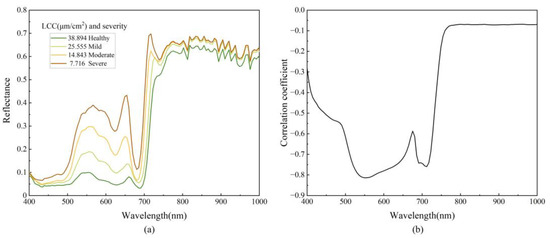
Figure 6.
(a) Spectral curves of the leaves with different degrees of disease; (b) Correlation between the LCC and spectrum.
3.2. Characteristic Wavelength Selection and Modeling
3.2.1. Characteristic Wavelength Selection
As shown in Figure 7a, the RMSE overall gradually decreases as the number of feature bands increases. The optimal subset comprises ten bands marked by red squares. This configuration indicates peak model performance. If F-tests suggest that the difference between the model’s RMSE and the actual minimum RMSE is insignificant, it suggests that the model performance is optimally tuned. Therefore, under these circumstances, adding more variables would only introduce redundancy and would not significantly improve model performance. Figure 7b illustrates that the selected feature bands are 449.58 nm, 510.17 nm, 550.95 nm, 592.04 nm, 628.25 nm, 675.15 nm, 690.87 nm, 727.72 nm, 780.78 nm, and 964.77 nm. This selection encompasses a limited but broadly distributed set of features, effectively minimizing the risk of overfitting. Notably, strong reflections in the green light at 550.95 and 592.04 nm, strong absorption in the red light at 675.15 nm, and the distinct red edge characteristics of the crops at 690.87 nm and 727.72 nm are well captured. These features are all strongly correlated with LCC.
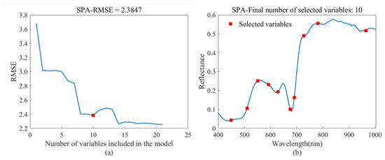
Figure 7.
(a) RMSE of SPA; (b) Characteristic bands selected by SPA.
3.2.2. Models Based on Spectral Features
The regression results of the two machine learning models based on full wavelengths and OWs selected via the SPA algorithm are listed in Table 5. Compared to the full wavelengths model, the OWs model shows a slight improvement in regression accuracy (Table 5). However, though the extent of this improvement is modest, model stability has not significantly increased. The phenomenon observed can be attributed to the band selection process, which, although it alleviates collinearity issues to some extent, also eliminates some potentially crucial information. This leads to a shortage of training features, consequently reducing the complexity of the trained model. The results indicate that the selected feature wavelengths can substitute for full wavelengths in predicting LCC.

Table 5.
Model results based on spectral features.
3.3. Vegetation Indices Selection and Modeling
3.3.1. Vegetation Indices Selection
In this study, we selected VIs for estimating LCC in mosaic leaves from 30 established vegetation indices. Figure 8 illustrates the MIC values of the 30 VIs. Utilizing the MIC, we identified nine VIs that demonstrated significant variability in their performance. Among these, CIgreen and GNDVI showed exceptionally similar and high performances (MIC = 0.7268), achieved through mathematical combinations of the green band at 550 nm and the red edge at 750 nm. Subsequent VIs, including NDRE, PSSRb, DD, MTCI, CIred-edge, and REP, exhibited MIC values of 0.6922, 0.6856, 0.6516, 0.6445, 0.6323, and 0.6064, respectively, all derived from formulas using red bands as members. The PRI, calculated using bands near the green peak at 531 nm and 570 nm, also displayed considerable correlation with an MIC of 0.5702.
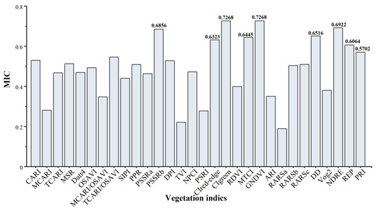
Figure 8.
The maximal information coefficient between 30 empirical VIs with LCC.
3.3.2. Models Based on Vegetation Indices
In this study, we used both unfiltered 30 VIs and 9 VIs selected through the MIC method as input parameters to estimate LCC, with the results detailed in Table 6. The BPNN model achieved the best training and validation scores using the full vegetation indices (RMSEC = 2.1494, R2C = 0.8556, RMSEV = 2.4880, R2V = 0.8014, RPDV = 2.2748). However, the SVR model demonstrated superior validation performance on the MIC-selected VIs (RMSE = 2.1444, R2 = 0.8532, RPDV = 2.6179). After applying the MIC method, the VIs demonstrate marked improvements in regression performance compared to the initial set of 30 VIs. With the selected VIs, the R2 values for the SVR, BPNN, and KNNR models in the validation set increased by 6.77%, 3.14%, and 6.50%, respectively. Concurrently, the RMSE values decreased by 0.4414, 0.1996, and 0.4043. Additionally, the prediction ability of the SVR and KNNR models exhibited substantial enhancements throughout the selection process, with the RPD exceeding 2.5. Such improvements indicate that the model has achieved a stable and reliable level of performance. These results suggest that not all empirical VIs initially listed contribute effectively to estimating LCC, confirming the efficacy of the MIC method in eliminating less effective parameters from the regression model.

Table 6.
Model results based on VIs.
3.4. Textural Feature Analysis and Modeling
3.4.1. Textural Feature Analysis
Figure 9 presents the textural feature contour plots for 480 hyperspectral samples. It is observed that although the variation patterns of textural features at different LCC levels are broadly similar, the sensitivity of individual features to LCC diverges. Notably, textural features such as MEA, VAR, and ENT exhibit a trend of increasing and then decreasing within certain wavelength ranges correlating with changes in LCC. Substantial shifts in the MEA suggest the extent of pigment damage. An increase in entropy suggests that the complexity and disorder of the leaf surface are escalating. At the same time, a rise in VAR denotes a broader variation and more detailed textural levels on the leaf surface. These alterations are often associated with the onset and spread of disease spots. Synthesizing this information, and selecting textural features that show a high degree of sensitivity to LCC changes can provide valuable insights for estimating LCC in apple leaves infected with mosaic disease.
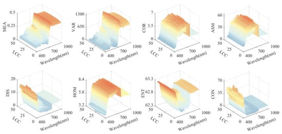
Figure 9.
Textural features of hyperspectral images across wavelengths with LCC concentration.
3.4.2. Textural Feature Construction and Selection
Figure 10 displays the MIC values of eight basic textural features across different OWs, indicating that the response intensity of basic textural features to LCC is closely linked to LCC-sensitive bands. The majority of textures have a weak correlation with LCC and most MIC values are less than 0.5. Notably, textures derived from the visible spectra demonstrate stronger correlations than those from the NIR spectra. The texture of red (628.25 nm) and yellow (592.04 nm) bands, in particular, exhibit the most pronounced correlations with LCC. Based on MIC values, the best band for each texture attribute was selected to represent the characteristic feature of that texture (MEA: 628.25 nm, VAR: 592.04 nm, COR: 628.25 nm, ASM: 628.25 nm, DIS: 628.25 nm, HOM: 628.25 nm, ENT: 628.25 nm, CON: 592.04 nm).
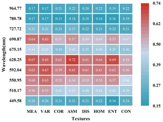
Figure 10.
MIC analysis results between basic textural features and LCC across OWs.
Given the moderate correlation between basic textural features and LCC, we computed NDTIs, DTIs, and RTIs for all pairwise combinations of these eight basic features. Figure 11 illustrates the correlation results considering textural indices and LCC based on the MIC method. Three kinds of textural indices demonstrate a stable correlation with LCC compared to a single textural attribute. The analyses of NDTIs and RTIs in relation to LCC yielded similar results, and both MEA and VAR exhibited significantly stronger correlations when paired with diverse texture attributes compared to other combinations. However, the MIC value of NDTIs is generally higher than that of RTIs. The MIC values for the relationship between DTIs and LCC indicate that most are above 0.5, with only a few low values. Particularly notable are the pairs including ASM or ENT, which produced even more similar and significant correlation results, with MIC values reaching up to 0.69.

Figure 11.
MIC analysis results between LCC and textural indices: (a) NDTIs; (b) DTIs; (c) RTIs.
3.4.3. Models Based on Textural Features
We input the textural information, which includes basic textures and three textural indices, into SVR, BPNN, and KNNR models to estimate LCC. Table 7 presents the evaluation results. The performance of the extracted significant basic texture model is notably inferior compared to the spectral feature model, with SVR, BPNN, and KNNR models achieving explanatory abilities of 66.63% (RMSE = 3.6088), 64.10% (RMSE = 3.7430), and 61.61% (RMSE = 3.8706), respectively. The values of RPD for all three models were below 1.8, suggesting single textural models can only provide a rough prediction of LCC. However, the textural indices demonstrate varying degrees of improvement in the assessment results compared to the basic texture models. The NDTIs had the best estimation effect, while SVR, BPNN, and KNNR exhibit a respective increase of 11.66%, 15.17%, and 14.77% in R2 on the validation set, accompanied by reductions in RMSE of 0.7996, 0.9977 and 0.9402, resulting in increased RPD, elevating prediction capabilities to around 2. DTIs and RTIs show only marginal improvements over the basic texture models across three machine learning models. However, as the RPD remains below 2, they fail to reach practical application levels. The phenomenon described above suggests that the combination of pairwise textural attributes overcomes the limitation of relying solely on basic feature inversion, mitigating the variability inherent in single feature regression by multidimensional explanation. Overall, textural features present certain potential in describing LCC on diseased leaves. However, single textural features for LCC estimation have their limitations. To comprehensively enhance the descriptive and informational dimensionality of LCC, integrating textural information with spectral information strengthens the depth of model interpretation.

Table 7.
Model results based on textural features.
3.4.4. Models Based on Combined Features
Spectral information (OWs, VIs) and textural information (Base-textures, NDTIs, DTIs, RTIs) were combined in five different ways to explore the evaluation impact of simple spectral and texture features, as well as feature indices after prior combinations of multiple indicators. After integrating spectral and textural information and subjecting them to collinearity filtering using the ReliefF algorithm, the selected results identified, as shown in Table 8, indicate a predominant contribution of spectral features within the fused features, with only a minority of textural features playing a decisive role.

Table 8.
Results after removing collinearity from combined features by ReliefF.
The final combined features serve as input parameters for SVR, BPNN, and KNNR models, and the outcomes are depicted in Figure 12. Overall, the combination of VIs and NDTIs attains the highest accuracy on the validation set, with R2 (0.8665) and RPD (2.7454) peaking, and RMSE (1.8871) reaching the minimum for the SVR model, showing a significant improvement over the best-performing spectral model using VIs (R2 = 0.8532, RMSE = 2.1444, RPD = 2.6179) alone. Next in line is the combination of VIs and basic textures, the SVR model achieved the best accuracy (R2 = 0.8589, RMSE = 2.0122, RPD = 2.6700). When using DTIs as an input predictor of the combined model, RMSE is decreased by 0.0794 for SVR than the VIs model. For the RTIs model, there was no significant improvement among the three machine learning models for LCC estimation than using VIs alone. In comparison, the combined model of OWs and basic textural features exhibits relatively poor accuracy; however, the BPNN (R2 = 0.8315, RMSE = 2.7032, RPD = 2.4381) achieved higher accuracy in terms of R2 and RPD compared to using OWs (R2 = 0.7844, RMSE = 2.3116, RPD = 2.2169) alone. It is evident that the response of the fusion content is more pronounced in terms of the three indicators. The combination of spectral and textural indices leverages the advantages of their respective features, enhancing the overall estimation performance by incorporating information from different dimensions.
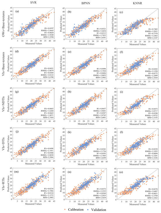
Figure 12.
Comparison of the measured LCC values and the estimated LCC values under SVR, BPNN, and KNNR models with input sets of combined OWs and Base-textures (a–c), combined VIs and Base-textures (d–f), combined VIs and NDTIs (g–i), combined VIs and DTIs (j–l), and combined VIs and RTIs (m–o).
3.5. Inversion of LCC by HSI
The best performing spectral model (VIs-SVR), textural model (NDTIs-BPNN), and spectra-texture combined model (VIs + NDTIs-SVR) were utilized to solve the hyperspectral images of apple mosaic leaves pixel by pixel, generating distribution maps of LCC, as shown in Figure 13. The selected range of LCC values for the leaves ranged from 0.87 to 34.86. Among the three models, both the VIs and VIs + NDTIs models accurately represented the distribution of different LCC levels. However, the combined model, incorporating spectral and textural indices guided by the SVR model (VIs + NDTIs) is closely aligned with the measured LCC range. Conversely, the textural features alone yielded subpar inversion results, providing only approximate delineations of the diseased areas. These findings are consistent with the performance evaluation results of the models.
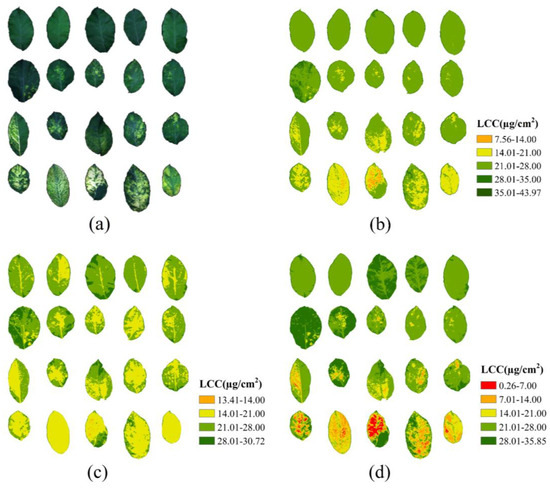
Figure 13.
(a) The measured hyperspectral images; (b) LCC distribution inverted through VIs model; (c) LCC distribution inverted through NDTIs model; (d) LCC distribution inverted through combination model (VIs + NDTIs).
4. Discussion
4.1. The LCC of Apple Leaves Infected with Mosaic Disease Exhibits Close Correlation with Spectral and Textural Features
The exacerbation of the disease visually manifests itself in changes in spot size, color, and morphology relative to healthy leaves. Still, it can only be used as an empirical criterion for rough disease identification. We found that LCC was consistently low in stressed leaf regions due to the evolution of fine regulatory mechanisms in plants facing virus invasion, which diverted more resources to activate the defense system to resist pathogen invasion at the expense of normal growth and development [79]. Therefore, rapid and accurate measurements of physiological indicators, such as LCC, are crucial for detecting plant diseases caused by viruses. Spectral information is widely utilized in HSI to evaluate the biochemical status of plants. Leaf pigmentation and cellular structure influence the dynamic changes in spectral reflectance, with healthy regions exhibiting low reflectance in the visible spectra and high reflectance in the NIR spectra [80]. When viruses infect leaves, a phenomenon known as the blue shift of red edge occurs, and the differences in absorption peaks and reflection valleys become particularly prominent for different LCC. Bands closely correlated with LCC in diseased leaves are more extensively distributed in the visible spectra. The maximum correlation coefficient reached −0.8135. These findings underscore the close relationship between spectral features and the disease condition. As leaves are infected by varying degrees of disease, their external morphological structures undergo diversified changes. These alterations can be described using textural features in HSI. Upon observation, it was noted that the eight basic textural attributes formed by GLCM exhibit diverse responses to the LCC. The MEA, VAR, and ENT among these textural features demonstrate particularly prominent roles within specific wavelength ranges. In certain visible bands, the MIC values between textural features and LCC reach 0.6, providing some guidance in inferring the LCC trend of diseased leaves. In summary, estimating the LCC of apple leaves infected with mosaic disease using spectral and textural features appears reasonable.
4.2. Comparative Analysis of Regression Models for Estimating LCC Using Spectral and Textural Features
After extracting 10 OWs and 9 VIs as spectral features, it was observed that the blue, green, and red bands are commonly utilized, underscoring their significance in estimating the LCC [77,81,82]. The prediction results of single and combined feature models are shown in Figure 14. We can see that VIs demonstrate more excellent capability than OWs, as they amalgamate variations from multiple spectral features, thereby minimizing redundancy in spectral data and enhancing plant spectral characteristics [83,84]. An analysis of the influence of basic textural features extracted by GLCM and three kinds of textural indices on LCC revealed that the effectiveness of textural feature models is generally weaker than models constructed using spectral features. Except for texture in the red and yellow bands, most textural features exhibit weak correlations with LCC, aligning with the findings of Wang et al. [85]. Incorporating two metrics into textural indices proves more advantageous for establishing LCC estimation models than basic textural features, as the organization of textural attributes enriches the expression of crop external characteristics. For apple mosaic disease, lesions harbor concealed information. Textural features with varying LCC display significant discrepancies across specific wavelength ranges. It suggests that utilizing sensitive indicators derived from these particular differences could enhance prediction accuracy. Therefore, estimating the LCC of apple mosaic leaves using spectral and textural features is justifiable.
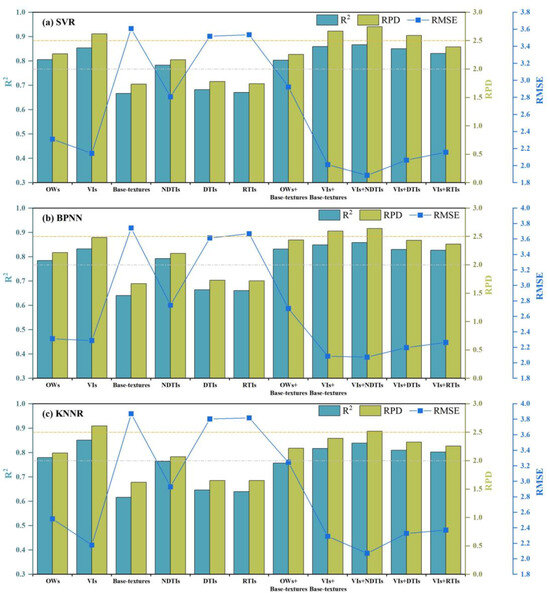
Figure 14.
Comparison of LCC values prediction results for apple mosaic leaves using single and combined feature models (a) SVR; (b) BPNN; (c) KNNR.
Building upon previous datasets of single spectral and textural features, representative variables were selected and combined to create input variables for machine learning models. Subsequently, combined feature models were developed to estimate LCC. The SVR model based on feature combination (VIs and NDTIs) attained the highest accuracy (R2 = 0.8665, RMSE = 1.8871, RPD = 2.7454) compared to all single feature models. Similarly, the BPNN and KNNR models combining VIs and NDTIs also achieved the highest accuracy in their respective comparisons. However, the accuracy of the combined model combining base-textures and OWs was lower. DTIs and RTIs perform relatively average as single textural features in this study, and their improvement in combination with VIs is also not particularly significant. This highlights that including members with low correlation may lead to a decrease in model accuracy while integrating indicators with higher correlation can enhance detection accuracy [61,86]. Therefore, selecting appropriate spectral and textural features is crucial for crop detection.
The conclusion drawn from the above findings suggests that the sensitivity of spectral features to leaf pigments and cellular structures enables a more detailed interpretation of LCC. While varying degrees of leaf lesions induce discernible changes in texture, the inherent variability of textures poses a challenge in accurately distinguishing these features on a quantitative scale, leading to less satisfactory outcomes in predicting biochemical parameters. The combined feature models provide a comprehensive analysis of apple leaves infected with mosaic disease, thus enhancing the accuracy of diagnosing diseased plants. Therefore, while textural features may not be suitable as independent remote sensing variables for estimating LCC, they can serve as supplementary variables to spectral features to achieve higher estimation accuracy [87]. For example, the combinations of NDTIs and VIs, DTIs and VIs, as well as base-textures and OWs, all show potential to improve estimation performance over individual spectral features.
Comparing SVR, BPNN, and KNNR models, the SVR model mostly yielded more stable and accurate results. This superiority may be attributed to the inherent stability and robustness of the SVR models in handling nonlinear regression problems. Therefore, based on the findings of this study, SVR emerges as the preferred algorithm for LCC inversion.
5. Conclusions
This study aims to explore the impact of feature parameters derived from two dimensions, spectral information (OWs, VIs) and textural information (Base-textures, NDTIs, DTIs, RTIs), extracted from hyperspectral images on estimating the LCC of apple leaves affected with mosaic disease. Additionally, our objective was to combine these two dimensions to develop quantitative inversion models using SVR, BPNN, and KNNR. The conclusions are as follows:
- (1)
- Samples with different LCC showed significant differences in spectral reflectance. Moreover, certain textural features under visible spectra, particularly MEA, VAR, and ENT showed a high correlation with LCC. Multi-metric aggregated VIs and NDTIs enhance feature differentiation;
- (2)
- Based on validation results from single feature models, spectral indices and textural indices, respectively, demonstrate optimal performance. Textural features, in general, exhibit inferior regression performance compared to spectral features and are unsuitable for independent applications;
- (3)
- Utilizing combined features as input parameters has the potential to enhance the estimation of LCC in apple mosaic leaves. However, the effectiveness of the combined approach was influenced by the performance of member variables. Ultimately, the SVR model combining NDTIs and VIs derived from the red and yellow bands exhibited the most accurate prediction of LCC (R2 = 0.8665, RMSE = 1.8871, RPD = 2.7454). This model outperformed the best-performing VIs model based on univariate parameters (R2 = 0.8532, RMSE = 2.1444, RPD = 2.6179);
- (4)
- Among the three machine learning methods used, the SVR model showed better estimation performance than the BPNN and KNNR models.
Author Contributions
Conceptualization, Z.S.; methodology, Z.S.; software, Z.S.; validation, Z.S. and Y.L.; formal analysis, Z.S. and Z.G.; investigation, Z.S., Y.L., J.Y., Y.G., D.J. and Y.Z.; resources, Q.C.; data curation, Z.S. and Y.L.; writing—original draft preparation, Z.S.; writing—review and editing, Z.S., D.J. and Y.Z.; visualization, Z.S. and Z.G.; supervision, Q.C.; project administration, Q.C.; funding acquisition, Q.C. All authors have read and agreed to the published version of the manuscript.
Funding
This research was funded by the National Natural Science Foundation of China (No. 41701398, No. 42071240).
Data Availability Statement
Data sharing is not applicable to this article.
Acknowledgments
We would like to thank all the students in Chang’s team for collecting the data for us.
Conflicts of Interest
The authors declare no conflicts of interest.
References
- Xing, F.; Wang, H.; Li, S. Advances in the Identification of Pathogens Associated with Apple Mosaic Disease of Apple Trees in China. J. Fruit Sci. 2021, 37, 1953–1963. [Google Scholar]
- Wu, C.; Niu, Z.; Tang, Q.; Huang, W. Estimating Chlorophyll Content from Hyperspectral Vegetation Indices: Modeling and Validation. Agric. For. Meteorol. 2008, 148, 1230–1241. [Google Scholar] [CrossRef]
- Mohammed, G.H.; Binder, W.D.; Gillies, S.L. Chlorophyll Fluorescence: A Review of Its Practical Forestry Applications and Instrumentation. Scand. J. For. Res. 1995, 10, 383–410. [Google Scholar] [CrossRef]
- Liu, Y.; Zhang, Y.; Jiang, D.; Zhang, Z.; Chang, Q. Quantitative Assessment of Apple Mosaic Disease Severity Based on Hyperspectral Images and Chlorophyll Content. Remote Sens. 2023, 15, 2202. [Google Scholar] [CrossRef]
- Zeng, J.; Ping, W.; Sanaeifar, A.; Xu, X.; Luo, W.; Sha, J.; Huang, Z.; Huang, Y.; Liu, X.; Zhan, B.; et al. Quantitative Visualization of Photosynthetic Pigments in Tea Leaves Based on Raman Spectroscopy and Calibration Model Transfer. Plant Methods 2021, 17, 4. [Google Scholar] [CrossRef] [PubMed]
- Sharma, M.; Jindal, V. Approximation Techniques for Apple Disease Detection and Prediction Using Computer Enabled Technologies: A Review. Remote Sens. Appl. Soc. Environ. 2023, 32, 101038. [Google Scholar] [CrossRef]
- Xu, T.; Wang, F.; Shi, Z.; Xie, L.; Yao, X. Dynamic Estimation of Rice Aboveground Biomass Based on Spectral and Spatial Information Extracted from Hyperspectral Remote Sensing Images at Different Combinations of Growth Stages. ISPRS J. Photogramm. Remote Sens. 2023, 202, 169–183. [Google Scholar] [CrossRef]
- Numata, I.; Roberts, D.A.; Chadwick, O.A.; Schimel, J.P.; Galvão, L.S.; Soares, J.V. Evaluation of Hyperspectral Data for Pasture Estimate in the Brazilian Amazon Using Field and Imaging Spectrometers. Remote Sens. Environ. 2008, 112, 1569–1583. [Google Scholar] [CrossRef]
- Zhou, X.; Zhao, C.; Sun, J.; Cao, Y.; Yao, K.; Xu, M. A Deep Learning Method for Predicting Lead Content in Oilseed Rape Leaves Using Fluorescence Hyperspectral Imaging. Food Chem. 2023, 409, 135251. [Google Scholar] [CrossRef]
- Zhao, R.; An, L.; Tang, W.; Qiao, L.; Wang, N.; Li, M.; Sun, H.; Liu, G. Improving Chlorophyll Content Detection to Suit Maize Dynamic Growth Effects by Deep Features of Hyperspectral Data. Field Crops Res. 2023, 297, 108929. [Google Scholar] [CrossRef]
- Wu, J.; Bai, T.; Li, X. Inverting Chlorophyll Content in Jujube Leaves Using a Back-Propagation Neural Network–Random Forest–Ridge Regression Algorithm with Combined Hyperspectral Data and Image Color Channels. Agronomy 2024, 14, 140. [Google Scholar] [CrossRef]
- Li, X.; Wei, Z.; Peng, F.; Liu, J.; Han, G. Estimating the Distribution of Chlorophyll Content in CYVCV Infected Lemon Leaf Using Hyperspectral Imaging. Comput. Electron. Agric. 2022, 198, 107036. [Google Scholar] [CrossRef]
- Gai, J.; Wang, J.; Xie, S.; Xiang, L.; Wang, Z. Spectroscopic Determination of Chlorophyll Content in Sugarcane Leaves for Drought Stress Detection. Precis. Agric. 2024, 25, 543–569. [Google Scholar] [CrossRef]
- Myneni, R.B.; Hall, F.G.; Sellers, P.J.; Marshak, A.L. The Interpretation of Spectral Vegetation Indexes. IEEE Trans. Geosci. Remote Sens. 1995, 33, 481–486. [Google Scholar] [CrossRef]
- Zhang, Y.; Xiao, J.; Yan, K.; Lu, X.; Li, W.; Tian, H.; Wang, L.; Deng, J.; Lan, Y. Advances and Developments in Monitoring and Inversion of the Biochemical Information of Crop Nutrients Based on Hyperspectral Technology. Agronomy 2023, 13, 2163. [Google Scholar] [CrossRef]
- Xue, L.; Yang, L. Deriving Leaf Chlorophyll Content of Green-Leafy Vegetables from Hyperspectral Reflectance. ISPRS J. Photogramm. Remote Sens. 2009, 64, 97–106. [Google Scholar] [CrossRef]
- Gitelson, A.A.; Viña, A.; Ciganda, V.; Rundquist, D.C.; Arkebauer, T.J. Remote Estimation of Canopy Chlorophyll Content in Crops. Geophys. Res. Lett. 2005, 32, L08403. [Google Scholar] [CrossRef]
- Dash, J.; Curran, P.J. The MERIS Terrestrial Chlorophyll Index. Int. J. Remote Sens. 2004, 25, 5403–5413. [Google Scholar] [CrossRef]
- Rao, N.R.; Garg, P.K.; Ghosh, S.K.; Dadhwal, V.K. Estimation of Leaf Total Chlorophyll and Nitrogen Concentrations Using Hyperspectral Satellite Imagery. J. Agric. Sci. 2008, 146, 65–75. [Google Scholar]
- Gao, C.; Li, H.; Wang, J.; Zhang, X.; Huang, K.; Song, X.; Yang, W.; Feng, M.; Xiao, L.; Zhao, Y.; et al. Combined Use of Spectral Resampling and Machine Learning Algorithms to Estimate Soybean Leaf Chlorophyll. Comput. Electron. Agric. 2024, 218, 108675. [Google Scholar] [CrossRef]
- Kira, O.; Linker, R.; Gitelson, A. Non-Destructive Estimation of Foliar Chlorophyll and Carotenoid Contents: Focus on Informative Spectral Bands. Int. J. Appl. Earth Obs. Geoinform. 2015, 38, 251–260. [Google Scholar] [CrossRef]
- Shu, M.; Fei, S.; Zhang, B.; Yang, X.; Guo, Y.; Li, B.; Ma, Y. Application of UAV Multisensor Data and Ensemble Approach for High-Throughput Estimation of Maize Phenotyping Traits. Plant Phenomics 2022, 2022, 9802585. [Google Scholar] [CrossRef] [PubMed]
- Pineda, M. An Overview of the Special Issue on Plant Phenotyping for Disease Detection. Remote Sens. 2021, 13, 4182. [Google Scholar] [CrossRef]
- Sun, J.; Jin, X.; Mao, H.; Wu, X.; Zhu, W.; Zhang, X.; Gao, H. Detection of Nitrogen Content in Lettuce Leaves Based on Spectroscopy and Texture Using Hyperspectral Imaging Technology. Trans. Chin. Soc. Agric. Eng. 2014, 30, 167–173. [Google Scholar]
- Zhang, X.; Zhang, K.; Sun, Y.; Zhao, Y.; Zhuang, H.; Ban, W.; Chen, Y.; Fu, E.; Chen, S.; Liu, J.; et al. Combining Spectral and Texture Features of UAS-Based Multispectral Images for Maize Leaf Area Index Estimation. Remote Sens. 2022, 14, 331. [Google Scholar] [CrossRef]
- Xie, C.; Wang, J.; Feng, L.; Liu, F.; Wu, D.; He, Y. Study on the Early Detection of Early Blight on Tomato Leaves Using Hyperspectral Imaging Technique Based on Spectroscopy and Texture. Spectrosc. Spectr. Anal. 2013, 33, 1603–1607. [Google Scholar]
- Yan, M.; Wang, H.; Wu, Y. Detection of Chlorophyll Content of Epipremnum Aureum Based on Fusion of Spectrum and Texture Features. J. Nanjing Agric. Univ. 2021, 44, 568–575. [Google Scholar]
- An, L.; Tang, W.; Qiao, L.; Zhao, R.; Sun, H.; Li, M.; Zhang, Y.; Zhang, M.; Li, X. Estimation of Chlorophyll Distribution in Banana Canopy Based on RGB-NIR Image Correction for Uneven Illumination. Comput. Electron. Agric. 2022, 202, 107358. [Google Scholar] [CrossRef]
- Cerovic, Z.G.; Masdoumier, G.; Ghozlen, N.B.; Latouche, G. A New Optical Leaf-clip Meter for Simultaneous Non-destructive Assessment of Leaf Chlorophyll and Epidermal Flavonoids. Physiol. Plant. 2012, 146, 251–260. [Google Scholar] [CrossRef]
- He, L.; Wan, L.; Gao, H. Recognition of Drought Stress in Tomato Based on Hyperspectral Imaging. Spectrosc. Spectr. Anal. 2023, 43, 724–730. [Google Scholar]
- Xiao, Q.; Tang, W.; Zhang, C.; Zhou, L.; Feng, L.; Shen, J.; Yan, T.; Gao, P.; He, Y.; Wu, N. Spectral Preprocessing Combined with Deep Transfer Learning to Evaluate Chlorophyll Content in Cotton Leaves. Plant Phenomics 2022, 2022, 9813841. [Google Scholar] [CrossRef] [PubMed]
- Yin, W.-J.; Ru, C.-L.; Zheng, J.; Zhang, L.; Yan, J.-Z.; Zhang, H. Fusion of Spectrum and Image Features to Identify Glycyrrhizae Radix et Rhizoma from Different Origins Based on Hyperspectral Imaging Technology. Chin. Mater. Medica 2021, 46, 923–930. [Google Scholar]
- Pan, Z.; Sun, G.; Zhang, A.; Fu, H.; Wang, X.; Ren, G. Tobacco Disease Detection Model Based on Band Selection. Spectrosc. Spectr. Anal. 2023, 43, 1023–1029. [Google Scholar]
- Araújo, M.C.U.; Saldanha, T.C.B.; Galvão, R.K.H.; Yoneyama, T.; Chame, H.C.; Visani, V. The Successive Projections Algorithm for Variable Selection in Spectroscopic Multicomponent Analysis. Chemom. Intell. Lab. Syst. 2001, 57, 65–73. [Google Scholar] [CrossRef]
- Deng, X.L.; Zeng, G.L.; Zhu, Z.H.; Huang, Z.X.; Yang, J.C.; Tong, Z.J.; Yin, X.B.; Wang, T.W.; Lan, Y.B. Classification and feature band extraction of diseased citrus plants based on UAV hyperspectral remote sensing. J. South. China Agric. Univ. 2020, 41, 100–108. [Google Scholar]
- Mao, F.; Sun, H.; Liu, H.; Zhang, J.; Li, M.; Yang, L. Prediction of Winter Wheat Chlorophyll Content Based on Gram-Schmidt and SPXY Algorithm. J. Agric. Mach. 2017, 48, 160–165. [Google Scholar]
- Galvao, R.; Araujo, M.; Jose, G.; Pontes, M.; Silva, E.; Saldanha, T. A Method for Calibration and Validation Subset Partitioning. Talanta 2005, 67, 736–740. [Google Scholar] [CrossRef] [PubMed]
- Wang, S.; Han, P.; Cui, G.; Wang, D.; Liu, S.; Zhao, Y. The NIR Detection Research of Soluble Solid Content in Watermelon Based on SPXY Algorithm. Spectrosc. Spectr. Anal. 2019, 39, 738–742. [Google Scholar]
- Kim, M.S.; Daughtry, C.; Chappelle, E.; McMurtrey, J.; Walthall, C. The Use of High Spectral Resolution Bands for Estimating Absorbed Photosynthetically Active Radiation (A Par). In CNES, Proceedings of the 6th International Symposium on Physical Measurements and Signatures in Remote Sensing, Val d’Isere, France, 17–24 January 1994; NASA: Washington, DC, USA, 1994. [Google Scholar]
- Daughtry, C. Estimating Corn Leaf Chlorophyll Concentration from Leaf and Canopy Reflectance. Remote Sens. Environ. 2000, 74, 229–239. [Google Scholar] [CrossRef]
- Haboudane, D.; Miller, J.R.; Tremblay, N.; Zarco-Tejada, P.J.; Dextraze, L. Integrated Narrow-Band Vegetation Indices for Prediction of Crop Chlorophyll Content for Application to Precision Agriculture. Remote Sens. Environ. 2002, 81, 416–426. [Google Scholar] [CrossRef]
- Chen, J.M. Evaluation of Vegetation Indices and a Modified Simple Ratio for Boreal Applications. Can. J. Remote Sens. 1996, 22, 229–242. [Google Scholar] [CrossRef]
- Datt, B. Remote Sensing of Chlorophyll a, Chlorophyll b, Chlorophyll A+b, and Total Carotenoid Content in Eucalyptus Leaves. Remote Sens. Environ. 1998, 66, 111–121. [Google Scholar] [CrossRef]
- Rondeaux, G.; Steven, M.; Baret, F. Optimization of Soil-Adjusted Vegetation Indices. Remote Sens. Environ. 1996, 55, 95–107. [Google Scholar] [CrossRef]
- Devadas, R.; Lamb, D.W.; Simpfendorfer, S.; Backhouse, D. Evaluating ten spectral vegetation indices for identifying rust infection in individual wheat leaves. Precis. Agric. 2009, 10, 459–470. [Google Scholar] [CrossRef]
- Metternicht, G. Vegetation Indices Derived from High-Resolution Airborne Videography for Precision Crop Management. Int. J. Remote Sens. 2003, 24, 2855–2877. [Google Scholar] [CrossRef]
- Blackburn, G.A. Spectral Indices for Estimating Photosynthetic Pigment Concentrations: A Test Using Senescent Tree Leaves. Int. J. Remote Sens. 1998, 19, 657–675. [Google Scholar] [CrossRef]
- Zarco-Tejada, P.J.; Pushnik, J.C.; Dobrowski, S.; Ustin, S.L. Steady-State Chlorophyll a Fluorescence Detection from Canopy Derivative Reflectance and Double-Peak Red-Edge Effects. Remote Sens. Environ. 2003, 84, 283–294. [Google Scholar] [CrossRef]
- Broge, N.H.; Leblanc, E. Comparing Prediction Power and Stability of Broadband and Hyperspectral Vegetation Indices for Estimation of Green Leaf Area Index and Canopy Chlorophyll Density. Remote Sens. Environ. 2001, 76, 156–172. [Google Scholar] [CrossRef]
- Peñuelas, J.; Gamon, J.A.; Fredeen, A.L.; Merino, J.; Field, C.B. Reflectance Indices Associated with Physiological Changes in Nitrogen- and Water-Limited Sunflower Leaves. Remote Sens. Environ. 1994, 48, 135–146. [Google Scholar] [CrossRef]
- Merzlyak, M.N.; Gitelson, A.A.; Chivkunova, O.B.; Rakitin, V.Y.U. Non-destructive Optical Detection of Pigment Changes during Leaf Senescence and Fruit Ripening. Physiol. Plant. 1999, 106, 135–141. [Google Scholar] [CrossRef]
- Gitelson, A.A.; Viña, A.; Arkebauer, T.J.; Rundquist, D.C.; Keydan, G.; Leavitt, B. Remote Estimation of Leaf Area Index and Green Leaf Biomass in Maize Canopies. Geophys. Res. Lett. 2003, 30, 1248. [Google Scholar] [CrossRef]
- Roujean, J.-L.; Breon, F.-M. Estimating PAR Absorbed by Vegetation from Bidirectional Reflectance Measurements. Remote Sens. Environ. 1995, 51, 375–384. [Google Scholar] [CrossRef]
- Gitelson, A.A.; Merzlyak, M.N.; Lichtenthaler, H.K. Detection of Red Edge Position and Chlorophyll Content by Reflectance Measurements Near 700 Nm. J. Plant Physiol. 1996, 148, 501–508. [Google Scholar] [CrossRef]
- Gitelson, A.; Merzlyak, M.; Zur, Y.; Stark, R.; Gritz, U. Non-Destructive and Remote Sensing Techniques for Estimation of Vegetation Status. Sch. Nat. Resour. Fac. Publ. 2001, 3543, 327–335. [Google Scholar]
- Chappelle, E.W.; Kim, M.S.; McMurtrey, J.E. Ratio Analysis of Reflectance Spectra (RARS): An Algorithm for the Remote Estimation of the Concentrations of Chlorophyll A, Chlorophyll B, and Carotenoids in Soybean Leaves. Remote Sens. Environ. 1992, 39, 239–247. [Google Scholar] [CrossRef]
- le Maire, G.; François, C.; Dufrêne, E. Towards Universal Broad Leaf Chlorophyll Indices Using PROSPECT Simulated Database and Hyperspectral Reflectance Measurements. Remote Sens. Environ. 2004, 89, 1–28. [Google Scholar] [CrossRef]
- Vogelmann, J.E.; Rock, B.N.; Moss, D.M. Red Edge Spectral Measurements from Sugar Maple Leaves. Int. J. Remote Sens. 1993, 14, 1563–1575. [Google Scholar] [CrossRef]
- Barnes, E.; Clarke, T.R.; Richards, S.E.; Colaizzi, P.; Haberland, J.; Kostrzewski, M.; Waller, P.; Choi, C.; Riley, E.; Thompson, T.L. Coincident Detection of Crop Water Stress, Nitrogen Status, and Canopy Density Using Ground Based Multispectral Data. In Proceedings of the International Conference on Precision Agriculture and Other Resource Management, Bloomington, MN, USA, 16–19 July 2000. [Google Scholar]
- Gamon, J.A.; Peñuelas, J.; Field, C.B. A Narrow-Waveband Spectral Index That Tracks Diurnal Changes in Photosynthetic Efficiency. Remote Sens. Environ. 1992, 41, 35–44. [Google Scholar] [CrossRef]
- Wang, D.; Li, R.; Liu, T.; Liu, S.; Sun, C.; Guo, W. Combining Vegetation, Color, and Texture Indices with Hyperspectral Parameters Using Machine-Learning Methods to Estimate Nitrogen Concentration in Rice Stems and Leaves. Field Crops Res. 2023, 304, 109175. [Google Scholar] [CrossRef]
- Yuan, W.; Meng, Y.; Li, Y.; Ji, Z.; Kong, Q.; Gao, R.; Su, Z. Research on Rice Leaf Area Index Estimation Based on Fusion of Texture and Spectral Information. Comput. Electron. Agric. 2023, 211, 108016. [Google Scholar] [CrossRef]
- Khan, I.H.; Liu, H.; Li, W.; Cao, A.; Wang, X.; Liu, H.; Cheng, T.; Tian, Y.; Zhu, Y.; Cao, W.; et al. Early Detection of Powdery Mildew Disease and Accurate Quantification of Its Severity Using Hyperspectral Images in Wheat. Remote Sens. 2021, 13, 3612. [Google Scholar] [CrossRef]
- Liu, B.; Shen, W.; Yue, Y.; Li, R.; Tong, Q.; Zhang, B. Combining Spatial and Spectral Information to Estimate Chlorophyll Contents of Crop Leaves with a Field Imaging Spectroscopy System. Precis. Agric. 2017, 18, 491–506. [Google Scholar] [CrossRef]
- Sudu, B.; Rong, G.; Guga, S.; Li, K.; Zhi, F.; Guo, Y.; Zhang, J.; Bao, Y. Retrieving SPAD Values of Summer Maize Using UAV Hyperspectral Data Based on Multiple Machine Learning Algorithm. Remote Sens. 2022, 14, 5407. [Google Scholar] [CrossRef]
- Zheng, H.; Cheng, T.; Zhou, M.; Li, D.; Yao, X.; Tian, Y.; Cao, W.; Zhu, Y. Improved Estimation of Rice Aboveground Biomass Combining Textural and Spectral Analysis of UAV Imagery. Precis. Agric. 2019, 20, 611–629. [Google Scholar] [CrossRef]
- Guo, W.; Gong, Z.; Gao, C.; Yue, J.; Fu, Y.; Sun, H.; Zhang, H.; Zhou, L. An Accurate Monitoring Method of Peanut Southern Blight Using Unmanned Aerial Vehicle Remote Sensing. Precis. Agric. 2024. [Google Scholar] [CrossRef]
- Yang, Y.; Zhang, X.; Gao, W.; Zhang, Y.; Hou, X. Improving Lake Chlorophyll-a Interpreting Accuracy by Combining Spectral and Texture Features of Remote Sensing. Environ. Sci. Pollut. Res. 2023, 30, 83628–83642. [Google Scholar] [CrossRef]
- Reshef, D.N.; Reshef, Y.A.; Finucane, H.K.; Grossman, S.R.; McVean, G.; Turnbaugh, P.J.; Lander, E.S.; Mitzenmacher, M.; Sabeti, P.C. Detecting Novel Associations in Large Data Sets. Science 2011, 334, 1518–1524. [Google Scholar] [CrossRef] [PubMed]
- Zhu, W.; Sun, Z.; Peng, J.; Huang, Y.; Li, J.; Zhang, J.; Yang, B.; Liao, X. Estimating Maize Above-Ground Biomass Using 3D Point Clouds of Multi-Source Unmanned Aerial Vehicle Data at Multi-Spatial Scales. Remote Sens. 2019, 11, 2678. [Google Scholar] [CrossRef]
- Doktor, D.; Lausch, A.; Spengler, D.; Thurner, M. Extraction of Plant Physiological Status from Hyperspectral Signatures Using Machine Learning Methods. Remote Sens. 2014, 6, 12247–12274. [Google Scholar] [CrossRef]
- Liang, D.; Guan, Q.; Huang, W.; Huang, L.; Yang, G. Remote Sensing Inversion of Leaf Area Index Based on Support Vector Machine Regression in Winter Wheat. Trans. Chin. Soc. Agric. Eng. 2013, 29, 117–123. [Google Scholar]
- Guo, J.; Zhang, J.; Xiong, S.; Zhang, Z.; Wei, Q.; Zhang, W.; Feng, W.; Ma, X. Hyperspectral Assessment of Leaf Nitrogen Accumulation for Winter Wheat Using Different Regression Modeling. Precis. Agric. 2021, 22, 1634–1658. [Google Scholar] [CrossRef]
- Rumelhart, D.E.; Hinton, G.E.; Williams, R.J. Learning Representations by Back-Propagating Errors. Nature 1986, 323, 533–536. [Google Scholar] [CrossRef]
- Ta, N.; Chang, Q.; Zhang, Y. Estimation of Apple Tree Leaf Chlorophyll Content Based on Machine Learning Methods. Remote Sens. 2021, 13, 3902. [Google Scholar] [CrossRef]
- Viscarra Rossel, R.A.; McGlynn, R.N.; McBratney, A.B. Determining the Composition of Mineral-Organic Mixes Using UV–Vis–NIR Diffuse Reflectance Spectroscopy. Geoderma 2006, 137, 70–82. [Google Scholar] [CrossRef]
- Zhang, J.; Wang, K.; Wang, R. Study on Hyperspectral Remote Sensing in Estimate Vegetation Leaf Chlorophyll Content. J. Shanghai Jiaotong Univ. 2003, 21, 74–80. [Google Scholar]
- Chen, F.-F.; Du, Z.-Y.; Liu, X.; Xie, L.; Chen, J.-S. Effect of Cucumber Mosaic Virus-Encoded 2b Protein on Photosynthesis and Chloroplast Structure of the Host Plant. Prog. Biochem. Biophys. 2007, 34, 889–896. [Google Scholar]
- Medina-Puche, L.; Tan, H.; Dogra, V.; Wu, M.; Rosas-Diaz, T.; Wang, L.; Ding, X.; Zhang, D.; Fu, X.; Kim, C.; et al. A Defense Pathway Linking Plasma Membrane and Chloroplasts and Co-Opted by Pathogens. Cell 2020, 182, 1109–1124.e25. [Google Scholar] [CrossRef] [PubMed]
- Peng, Z.; Guan, L.; Liao, Y.; Lian, S. Estimating Total Leaf Chlorophyll Content of Gannan Navel Orange Leaves Using Hyperspectral Data Based on Partial Least Squares Regression. IEEE Access 2019, 7, 155540–155551. [Google Scholar] [CrossRef]
- Sonobe, R.; Wang, Q. Towards a Universal Hyperspectral Index to Assess Chlorophyll Content in Deciduous Forests. Remote Sens. 2017, 9, 191. [Google Scholar] [CrossRef]
- Wen, P.-F.; He, J.; Ning, F.; Wang, R.; Zhang, Y.-H.; Li, J. Estimating Leaf Nitrogen Concentration Considering Unsynchronized Maize Growth Stages with Canopy Hyperspectral Technique. Ecol. Indic. 2019, 107, 105590. [Google Scholar] [CrossRef]
- Xiao, B.; Li, S.; Dou, S.; He, H.; Fu, B.; Zhang, T.; Sun, W.; Yang, Y.; Xiong, Y.; Shi, J.; et al. Comparison of Leaf Chlorophyll Content Retrieval Performance of Citrus Using FOD and CWT Methods with Field-Based Full-Spectrum Hyperspectral Reflectance Data. Comput. Electron. Agric. 2024, 217, 108559. [Google Scholar] [CrossRef]
- Shah, S.H.; Angel, Y.; Houborg, R.; Ali, S.; McCabe, M.F. A Random Forest Machine Learning Approach for the Retrieval of Leaf Chlorophyll Content in Wheat. Remote Sens. 2019, 11, 920. [Google Scholar] [CrossRef]
- Wang, R.; Tuerxun, N.; Zheng, J. Improved Estimation of SPAD Values in Walnut Leaves by Combining Spectral, Texture, and Structural Information from UAV-Based Multispectral Image. Sci. Hortic. 2024, 328, 112940. [Google Scholar] [CrossRef]
- Patel, M.K.; Ryu, D.; Western, A.W.; Suter, H.; Young, I.M. Which Multispectral Indices Robustly Measure Canopy Nitrogen across Seasons: Lessons from an Irrigated Pasture Crop. Comput. Electron. Agric. 2021, 182, 106000. [Google Scholar] [CrossRef]
- Guo, A.; Huang, W.; Ye, H.; Dong, Y.; Ma, H.; Ren, Y.; Ruan, C. Identification of Wheat Yellow Rust Using Spectral and Texture Features of Hyperspectral Images. Remote Sens. 2020, 12, 1419. [Google Scholar] [CrossRef]
Disclaimer/Publisher’s Note: The statements, opinions and data contained in all publications are solely those of the individual author(s) and contributor(s) and not of MDPI and/or the editor(s). MDPI and/or the editor(s) disclaim responsibility for any injury to people or property resulting from any ideas, methods, instructions or products referred to in the content. |
© 2024 by the authors. Licensee MDPI, Basel, Switzerland. This article is an open access article distributed under the terms and conditions of the Creative Commons Attribution (CC BY) license (https://creativecommons.org/licenses/by/4.0/).