Article

Resilient Factor Graph-Based GNSS/IMU/Vision/Odo Integrated Navigation Scheme Enhanced by Noise Approximate Gaussian Estimation in Challenging Environments

1
Beijing Kunpeng Borui Technology Co., Ltd., Beijing 100096, China
2
School of Instrument Science and Engineering, Southeast University, Nanjing 210096, China
3
Key Laboratory of Micro-Inertial Instruments and Advanced Navigation Technology, Ministry of Education, Southeast University, Nanjing 210096, China
4
China Astronaut Research and Training Center, Beijing 100094, China
5
State Key Laboratory of Satellite Navigation System and Equipment Technology, The 54th Research Institute of China Electronics Technology Group Corporation, Shijiazhuang 050002, China
*
Author to whom correspondence should be addressed.
Remote Sens. 2024, 16(12), 2176; https://doi.org/10.3390/rs16122176
Submission received: 30 April 2024 / Revised: 9 June 2024 / Accepted: 14 June 2024 / Published: 15 June 2024
(This article belongs to the Special Issue Geospatial Artificial Intelligence (GeoAI) in Remote Sensing)

Abstract

:
The signal blockage and multipath effects of the Global Navigation Satellite System (GNSS) caused by urban canyon scenarios have brought great technical challenges to the positioning and navigation of autonomous vehicles. In this paper, an improved factor graph optimization algorithm enhanced by a resilient noise model is proposed. The measurement noise is resilient and adjusted based on an approximate Gaussian distribution-based estimation. In estimating and adjusting the noise parameters of the measurement model, the error covariance matrix of the multi-sensor fusion positioning system is dynamically optimized to improve the system accuracy. Firstly, according to the approximate Gaussian statistical property of the GNSS/odometer velocity residual sequence, the measured data are divided into an approximate Gaussian fitting region and an approximate Gaussian convergence region. Secondly, the interval is divided according to the measured data, and the corresponding variational Bayesian network and Gaussian mixture model are used to estimate the innovation online. Further, the noise covariance matrix of the adaptive factor graph-based model is dynamically optimized using the estimated noise parameters. Finally, based on low-cost inertial navigation equipment, GNSS, odometer, and vision, the algorithm is implemented and verified using a simulation platform and real-vehicle road test. The experimental results show that in a complex urban road environment, compared with the traditional factor graph fusion localization algorithm, the maximum improvement in accuracy of the proposed algorithm can reach 65.63%, 39.52%, and 42.95% for heading, position, and velocity, respectively.

1. Introduction

Accurate, reliable, and continuous navigation and localization are the important foundation and prerequisite for the safe operation of autonomous vehicles [1]. Localization can be further divided into absolute localization, relative localization, and simultaneous localization and mapping (SLAM) [2,3]. The Real-Time Kinematic-based Global Navigation Satellite System (RTK-GNSS) is the most widely applied localization technology for autonomous driving, but it is susceptible to interference in urban road environments [4,5]. The fusion of multi-sensor data can achieve complementary advantages and collaborative superiority to a certain extent, which is the core technology solution used to improve the perception capability of autonomous vehicles [6]. The inertial navigation system (INS)/GNSS/odometer fusion localization is the most commonly used navigation and localization technology for autonomous vehicles in urban road environments [7]. The INSs installed on autonomous vehicles are mostly based on lost-cost inertial measurement units (IMU). However, in GNSS-denied or challenging environments, the IMU/odometer standalone navigation system struggles to maintain long-term accuracy due to error accumulation [8,9]. Owing to the good autonomy of visual navigation, the visual/map attitude matrix measurement information can decouple the IMU/odometer measurement information, improving the system observability [10]. Additionally, visual feature matching is also an effective method used to improve the accuracy of IMU/odometer localization [11]. Based on the complementary characteristics between inertial navigation, odometry, satellite navigation, and vision, the multi-sensor data fusion module estimates and compensates navigation errors online through model state estimation, which can effectively improve the performance of the navigation system.
The complex urban road environment often has a significant impact on satellite navigation, for example, when differential data are unavailable due to communication abnormalities, the working state will be downgraded from RTK to single-point positioning (SPP); the signal obstruction and multipath effects caused by challenging environments (CEs) such as dense tree canopies, tall buildings, and overpasses will further increase or even interrupt the error. The frequent switching of satellite navigation working states caused by the dynamic changes in the urban environment will bring significant measurement model noise parameter errors, thereby significantly reducing the system accuracy. The nonlinear motion of carriers in congested environments poses a severe challenge to the performances of inertial devices. Laser radar and vision systems are also highly susceptible to the influence of the physical characteristics of the urban environment, typically manifested as model mismatches characterized by faults and biases. The mutual propagation and coupling of multi-sensor errors have exacerbated the complexity of the problem, making it difficult to meet the requirements of future autonomous vehicles for positioning accuracy, integrity, and continuity [12]. To address the challenges faced by the multi-sensor fusion localization systems of autonomous vehicles, scholars from various countries have made substantial research progress in recent years, which can be mainly divided into two directions [13,14]: (1) innovative distributed multi-source heterogeneous sensor fusion architectures, such as the fusion of GNSS, INS, odometry, and vision, to improve the performance of the integrated navigation system; and (2) research on optimized data fusion algorithms, such as improved Kalman filter series and factor graph (FG) optimization, to continuously enhance the performance of the fusion localization system.
In multi-sensor fusion localization systems of autonomous vehicles, the GNSS not only provides the only absolute positioning observation, but the high-precision RTK positioning data also plays a crucial role. However, in complex urban road environments, issues such as increased GNSS errors and signal interruptions inevitably degrade the accuracy of the fusion localization system. In improving the performance of the multi-sensor fusion localization system, the adaptive optimization of the GNSS measurement noise model has always been an important research direction. On road sections where multiple satellite navigation working modes alternate, the noise parameters based on empirical values will introduce non-negligible errors to the measurement model. The measurement data noise model error is one of the main factors limiting the improvement of the multi-sensor fusion localization accuracy.
Based on the resilient Positioning, Navigation and Timing (PNT) theory, it is necessary to perform the online accurate estimation and resilient adjustment of the noise model [15]. In order to overcome the problem of the decreased accuracy of integrated navigation systems caused by noise model parameter errors in complex urban road environments, this paper proposes an adaptive factor graph (AFG) data fusion optimization model enhanced by a resilient noise model. The noise is resilient and adjusted based on the approximate Gaussian estimation algorithm to effectively improve the accuracy of the IMU/GNSS/vision/odometer fusion localization system. First, the distribution characteristics of the GNSS measurement noise model were analyzed. Then, an algorithm for estimating the noise parameters based on the GNSS/odometer ground speed residual sequence was studied. Finally, an adaptive factor graph model enhanced by the resilient noise model was utilized to implement and test the system. The main contributions can be summarized as follows:
(1)
In using the velocity data output from the odometer as the reference, the approximate Gaussian distribution characteristics of the GNSS/Odometer ground speed residual sequence are analyzed.
(2)
Based on the variational Bayesian network and Gaussian mixture model (GMM), an approximate Gaussian estimation algorithm for the measurement data noise model is studied, and a resilient noise model is proposed.
(3)
Based on the resilient noise model, the factor graph-based IMU/GNSS/odometer/vision fusion navigation system is implemented, and the superiority of the algorithm is verified through theoretical analyses and road tests.
The rest of this paper is organized as follows. In Section 2, related research work is introduced. In Section 3, the proposed resilient noise model based on approximate Gaussian estimation is presented in detail. In Section 4, the factor graph-based IMU/GNSS/odometer/vision integrated navigation method enhanced by the resilient noise model is studied and presented. As discussed in Section 5, the superiority of the proposed algorithm was verified through simulation platform and road tests. Finally, the contributions of this study are discussed and summarized in the Conclusion.

2. Related Work and Problem Statement

Accurate and assured positioning results are crucial for safety-critical applications such as autonomous driving. However, in complex urban road environments, a single sensor struggles to achieve accurate and reliable environmental perception, and multi-source data fusion is an important research direction in the field of autonomous driving [16]. Meanwhile, the multiple localization sensors integrated in autonomous vehicles have distributed installation, asynchronous, and delayed characteristics, and the factor graph data fusion algorithm has obvious advantages. The related work is introduced in the following subsections from the aspects of factor graph data fusion algorithms and noise model optimization.

2.1. Multi-Source Fusion Localization Based on Factor Graph

The continuous improvement and optimization of the Kalman filter have improved the filter’s performance in terms of nonlinearity, adaptability, robustness, and fault tolerance [17,18]. However, the inherent defects limit the further improvement of their performance. The factor graph optimization algorithm based on the sum–product algorithm proposed by Kschischang [19] has many advantages, such as plug-and-play and global optimization, which can effectively solve the shortcomings of the Kalman filtering algorithm. Different from the Kalman-based filters, the factor graph optimization algorithm is based on the current data and historical data, and it achieves global optimization through the construction of a batch optimization cost function.
Zeng [20] studied an improved multi-sensor data fusion algorithm based on the factor graph, which fully utilizes the sensor data with different update rates, including inertial navigation, Global Positioning System (GPS), geomagnetic, vision, and sonar data, to achieve a globally optimal estimation. The effectiveness of this algorithm was verified through a comparison with that of the extended Kalman filter (EKF), and it was also tested on a small unmanned aerial vehicle platform. Furthermore, Wen [21] researched the tightly coupled GNSS/SINS integration based on the factor graph and fisheye camera and conducted a detailed comparison of the filtering effects of the EKF and factor graph in both loosely coupled and tightly coupled cases. The impact of the sliding window size on the factor graph filtering performance was also analyzed [22]. In the field of autonomous driving, Zhao [23] designed a sliding window smoothing estimator based on the factor graph architecture and applied it to the tightly coupled Differential GPS (DGPS)/inertial measurement unit (IMU) system on the Google self-driving car platform. Road tests in urban environments showed that this algorithm has significant advantages over the EKF, due to its global optimization, re-linearization, and multiple iterations. Gao [24] utilized the factor graph model to design a multi-source fusion localization algorithm, which effectively reduced the errors caused by the asynchrony and time delay of the sensors in the vehicle-mounted INS/GNSS/odometer system. Li [25] analyzed the advantages of the graph optimization algorithm over the EKF and proposed a robust graph optimization scheme for inertial/satellite tight integration, using the GNSS reliability state variable to optimize the GNSS pseudorange residual weight, thereby improving the system accuracy in urban road environments.

2.2. Adaptive Optimization of Measurement Noise Model

In complex urban road environments, autonomous vehicles face dynamic changes in navigation and positioning environments. Fixed noise parameters based on empirical values in multi-sensor fusion positioning systems inevitably introduce model errors. Conducting research on dynamic noise parameter estimation for multi-sensor data fusion models is an effective method for improving the positioning accuracy. Sarkka [26] first proposed the application of the variational Bayesian method to optimize measurement noise model parameters. In using fixed-point iterations, the noise variance distribution is statistically analyzed, improving the accuracy of the adaptive Kalman filtering. Li [27] achieved the adaptive optimization of the unscented Kalman filter (UKF) by performing a variational Bayesian approximate estimation of the model noise, improving the system’s robustness. To enhance the robustness of the Strap-down Inertial Navigation System (SINS)/GPS combined navigation system in complex environments, Hu [28] used the T-distribution to simulate the noise matrix, suppressing the heavy-tailed characteristics of noise caused by outliers. The variational Bayesian network was then used to iteratively estimate the state variables.
Optimally estimating measurement noise parameters based on innovation is an effective way to improve the performance of multi-sensor fusion localization systems. To enhance the positioning accuracy of autonomous driving systems in urban roads, Liu [29] proposed an online estimation method for measurement noise parameters using estimated values and measurements. The noise covariance matrix is updated and adaptively optimized through a decay factor, which more accurately reflects the noise characteristics and achieves the effect of suppressing white noise, effectively improving the accuracy of the INS/GPS fusion localization system. Addressing the issue of the reduced filter accuracy caused by uncertain statistical characteristics of the measurement noise, Yue [30] proposed a weighted adaptive square root cubature Kalman filter (CKF). The moving window theory is used to perform a maximum likelihood estimation (MLE) on the covariance matrix of innovation, based on which the measurement noise matrix is dynamically adjusted. This effectively improves the adaptive ability and navigation performance of the GPS/INS combined navigation system in environments with uncertain measurement noise statistics. Xu [31] performed a maximum a posteriori estimation of the covariance matrix of the factor graph data fusion model based on the estimated state values and observations and iteratively updated it through dynamic weighting, effectively improving the robustness of the multi-sensor fusion localization algorithm. By analyzing the raw observations of a GNSS and accelerometers, Jing [32] constructed an adaptive measurement noise model using the a posteriori coordinate covariance of an RTK-GNSS and optimized and improved the GNSS/odometer data fusion model. The batch covariance estimation (BCE) framework iteratively updates the measurement error uncertainty model by fitting the Gaussian mixture model to the measurement residuals, thereby achieving a robust state estimation of the robot platform. Watson [33] proposed the BCE-AD method by expanding the data space to achieve a more accurate description of measurement uncertainty models.
In summary, the aforementioned research on multi-sensor fusion localization has extensively explored optimization techniques for factor graph fusion algorithms from the perspectives of sensor schemes, data fusion architectures, and robustness. However, there are relatively few studies on the online adaptive optimization of covariance matrices. On the other hand, certain algorithms, such as variational Bayesian and maximum a posteriori algorithms, have been used to estimate system measurement information online, achieving the adaptive optimization of noise models. However, due to the lack of high-precision data with strong autonomy, the decoupling of noise model errors and measurement errors is difficult, and the accuracy needs to be further improved. Based on the advantages of odometry in terms of ground speed autonomy and accuracy, this paper proposes a noise parameter approximate Gaussian estimation method using the GNSS/odometer ground speed residual sequence as measurement information. After analyzing the distribution characteristics, the proposed method realizes an online resilient adjustment of the factor graph covariance matrix.

3. Approximate Gaussian Estimation of Measurement Noise Parameters Based on Innovation

To address the issue of system accuracy degradation caused by measurement noise model errors, a resilient noise model based on approximate Gaussian estimation is proposed in this section.

3.1. Approximate Gaussian Distribution Analysis of GNSS/Odometry Velocity Residual Sequences

As mentioned above, the GNSS is the most widely used positioning sensor for autonomous vehicles. However, it is also the most susceptible to interference in urban road environments, which can negatively impact the performances of combined navigation systems. Therefore, measurement noise model optimization primarily focuses on the online estimation of the impact of road environment changes on GNSS data. Odometry is an important autonomous sensor for relatively good accuracy in its output ground speed data. In using the ground speed output of the odometer as a reference, the estimation of the GNSS/odometer ground speed residual sequence can further improve the estimation accuracy of the measurement noise model. The expression for the velocity measurement output by the odometer in the vehicle coordinate system is shown in Equation (1):
v ˜ O D m = C m b 1 + δ K v O D + n O D
where v ˜ O D m represents the measured value of odometer; C m b represents the rotation matrix from the odometer body coordinate system to the vehicle body coordinate system; δ K represents the scale factor error; v O D represents the theoretical output value of the odometer; and n O D represents the Gaussian noise. In Equation (1), C m b can be neglected due to mechanical mounting and high-precision offline calibration; δ K can also be ignored after estimation and correction using RTK-GNSS road sections. Therefore, v ˜ O D m can be approximated as the sum of v O D and n O D . The mean and variance of the noise n O D are primarily affected by road factors such as bumps and slipping.
In considering that the odometer is typically mounted centrally on the non-steering wheel axle and that the GNSS antenna is centrally mounted on the roof, the lever arm effect between the two can be neglected. In using the odometer velocity as the GNSS velocity measurement estimate, the GNSS/odometry velocity residual sequence can be expressed as shown in Equation (2):
Z ˜ k / k 1 = Z ˜ Z ^ k / k 1 = δ V ˜ G N S S = v E + δ v E 2 + v N + δ v N 2 v E 2 + v N 2 n O D = 2 v E δ v E + 2 v N δ v N + δ v E 2 + δ v N 2 v E + δ v E 2 + v N + δ v N 2 + v E 2 + v N 2 n O D
where δ V ˜ G N S S represents the GNSS velocity residual sequence; v E represents the east velocity of the GNSS; and v N represents the north velocity of the GNSS. From Equation (2), it can be seen that the measurement noise of the velocity residual sequence does not follow a Gaussian distribution. When the vehicle is stationary, the true velocity value is 0, and the measurement noise becomes δ v E 2 + δ v N 2 n O D , which follows the difference between the Rayleigh distribution ( δ v E 2 + δ v N 2 ) and the Gaussian distribution ( n O D ). When v δ v , Equation (2) can be approximated as the sum of three Gaussian distributions. These two cases are shown in Equation (3):
δ V ˜ G N S S = δ v E 2 + δ v N 2 n O D ; v = 0 δ V ˜ G N S S v E δ v E v E 2 + v N 2 + v N δ v N v E 2 + v N 2 n O D ; v δ v
When the vehicle speed is between these two cases, Equation (2) can be represented as a mixed distribution, as shown in Equation (4):
δ V ˜ G N S S v E δ v E v E 2 + v N 2 + v N δ v N v E 2 + v N 2 + δ v E 2 + δ v N 2 2 v E 2 + v N 2 n O D
Figure 1 provides a concise illustration of the evolution process of the aforementioned residual sequence distribution characteristics. In Figure 1, δ represents the root mean square error (RMSE) of the east and north velocity measurements. As the velocity gradually increases from 0, the probability density function (PDF) of the measurement noise evolves from the Rayleigh distribution shown in PDF1 to the approximate Gaussian distribution shown in PDF5. In the three sets of data, PDF1, PDF2, and PDF3, the RMSE was set to 0.3 m/s, and the distribution characteristics gradually evolved toward the Gaussian distribution as the velocity increased. At the same time, in the two sets of data, PDF3 and PDF4, the velocity value was 3.754 m/s, and when the RMSE was reduced from 0.3 m/s to 0.03 m/s, the distribution characteristics became closer to the Gaussian distribution. This shows that as the error-to-true value ratio decreases, the measurement noise error model will gradually evolve from a Rayleigh distribution to an approximate Gaussian distribution.
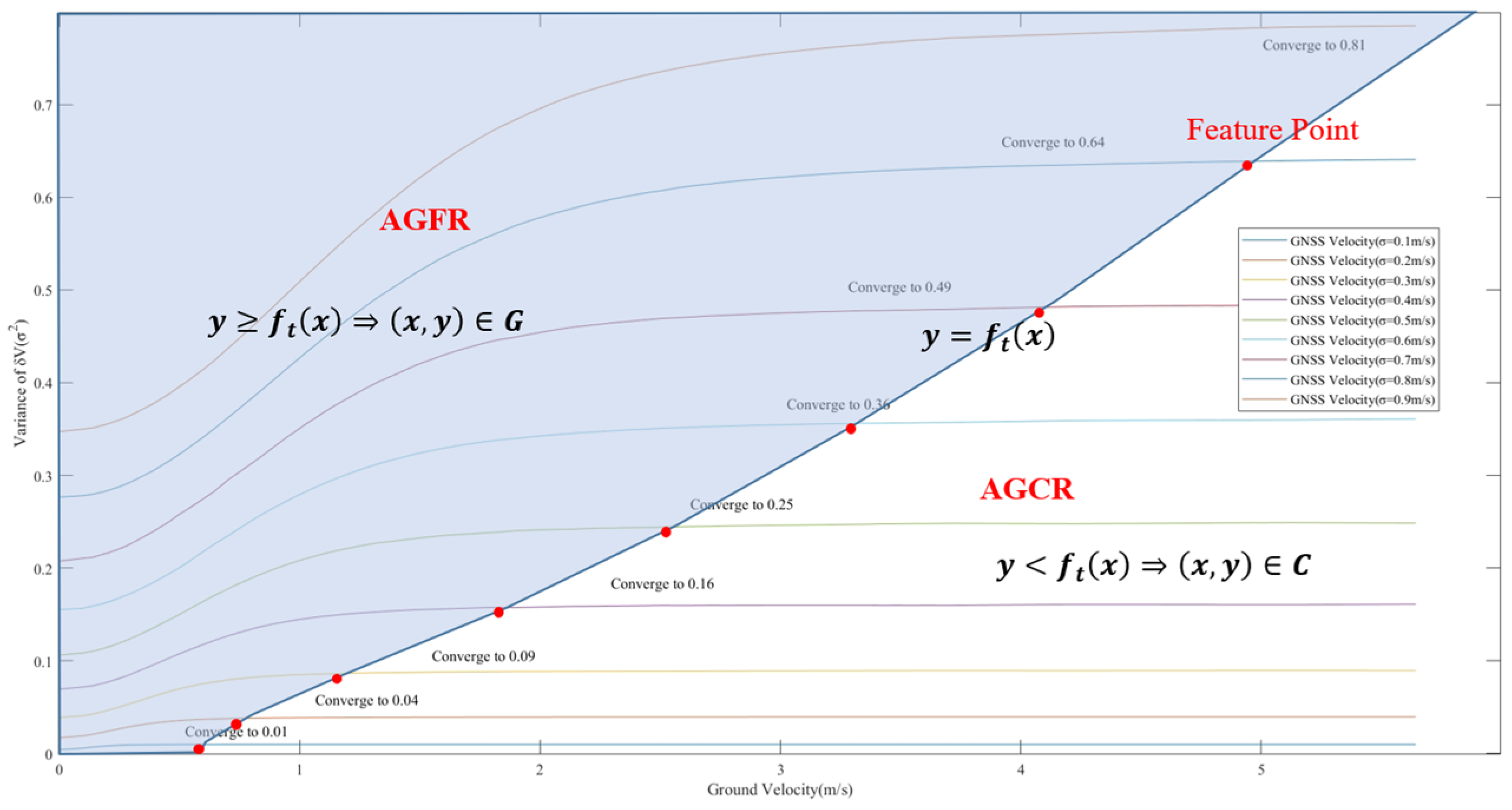
In our previous research [34], using a simulation platform, we conducted a detailed analysis of the changes in the velocity and variance function relationship curves during the uniform acceleration of a vehicle from [0 m/s, 0 m/s] to [6 m/s, 3 m/s] for nine sets of GNSS velocity RMSE values. The results are shown in Figure 2.
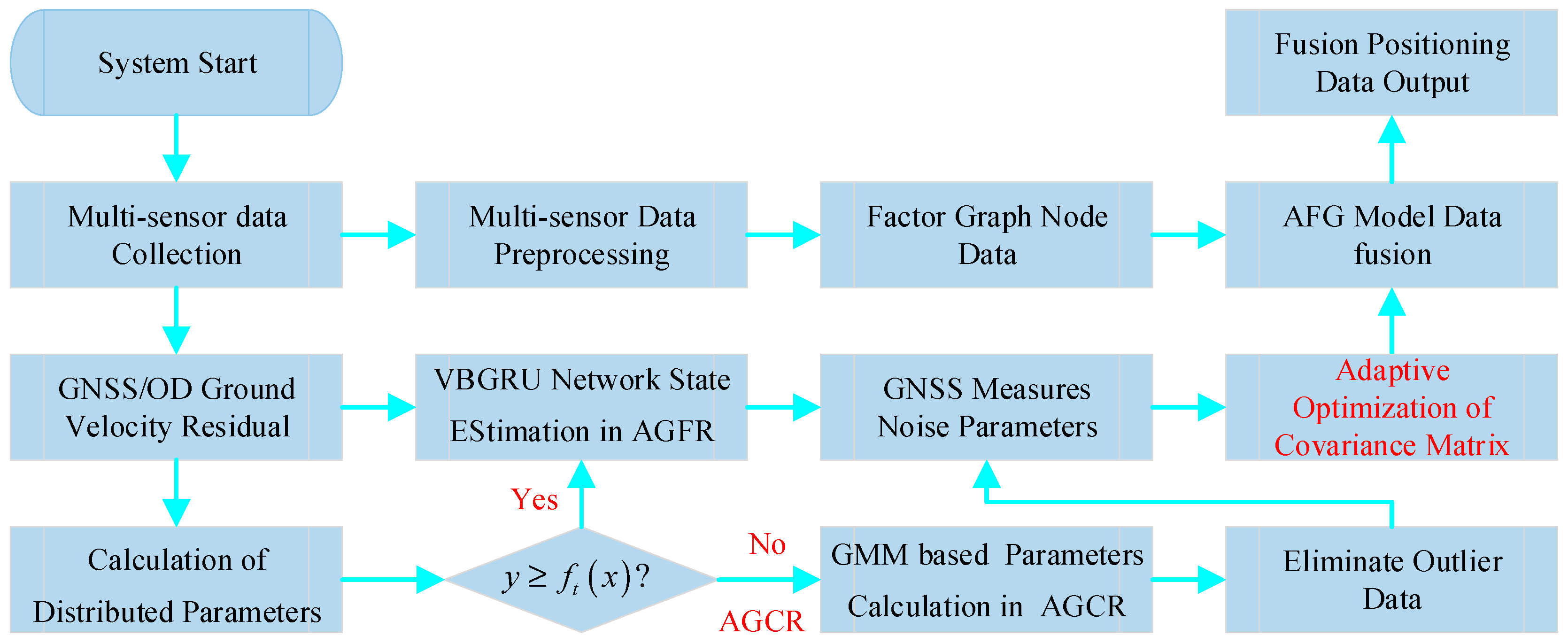
Based on the vehicle speed and innovation data distribution characteristics in Figure 2, a convergence function y = f t x is fitted, and the data regions satisfying the relationship, y f t x and y < f t x , are divided into the AGFR and the AGCR, respectively. In the AGFR, the nonlinearity of the speed and variance relationship function is relatively strong, and a neural network is suitable for fitting and solving. In the AGCR, the information sequence has converged, and it can be estimated according to the Gaussian distribution. In conventional autonomous driving scenarios, the data sequence distribution characteristics are basically consistent, and the mean and variance parameters can be estimated using the MLE method based on the given sufficient measurement dataset. However, in complex urban road positioning environments, RTK, GNSS single-point positioning, and GNSS challenging environment navigation states appear alternately, and the sample set formed by the information sequence within the time window may contain multiple Gaussian mixture distributions. In challenging environments, GNSS measurement data can bring significant errors to the state estimation model. Using a GMM to solve multiple sub-distributions of data within the window and eliminate outliers can further optimize the adaptive factor graph model. Based on the above analysis, the main calculation process of the multi-sensor fusion positioning system based on the approximate Gaussian noise model estimation is shown in Figure 3.

3.2. The Design of Resilient Noise Model Based on the Approximate Gaussian Estimation Algorithm

The distribution characteristics of the innovation sequence dynamically change between the Rayleigh distribution and approximate Gaussian distribution according to the driving speed and road environment changes of autonomous vehicles. The functional relationships between speed, innovation, and GNSS measurement noise parameters are divided into the AGFR and AGCR, and they are solved using a variational Bayesian network and GMM, respectively. The two algorithms are described in detail as follows.

3.2.1. Variational Bayesian Network Estimation of Noise Parameters Based on Innovation

Each nonlinear function curve in the AGFR corresponds to a specific speed measurement root mean square error, which essentially reflects the relationship between the change in ground speed variance with the increase in speed under different speed measurement root mean square error conditions. Therefore, the output result corresponding to each data group is not only related to the current value but also has a relationship with the previous and subsequent data. Based on the obvious advantages of the Gate Recurrent Unit (GRU) framework–deep neural network in sequence data processing, this network was selected for the measurement noise parameter estimation.
The variational Bayesian GRU (VBGRU) network combines the characteristics of variational Bayesian Inference (VBI) and the GRU network, introducing uncertainty weights into the model training process, representing model parameters with random variables of normal distribution, which greatly improves the adaptability and generalization ability of the model. Different from the traditional GRU network, the VBGRU uses random variables of a specific probability density distribution to fit nonlinear functions. At the same time, it can calculate its uncertainty while outputting the predicted value, which is a maximum a posteriori estimation method.
As the multi-sensor fusion positioning system is carried out on the autonomous driving edge computing platform, the real-time calculation performance of the algorithm is particularly important. Therefore, the VBGRU network adopts a lightweight three-layer Long Short-Term Memory (LSTM) architecture design, with the number of neurons being 48, 48, and 24, respectively; the decoder adopts a two-layer LSTM architecture, with the number of neurons being 24 and 24, respectively. Reference [33] conducted an experimental verification of the network through a simulation platform, and its accuracy could meet the measurement noise estimation requirements of urban roads.

3.2.2. Noise Parameter Estimation Based on Innovation and Gaussian Mixture Model

The essence of the GMM is to decompose a probability density function that conforms to the characteristics of a Gaussian distribution into multiple Gaussian functions. Its random variables can be either one-dimensional or multi-dimensional, which can be specifically expressed as shown in Equation (5):
f x = k = 1 M λ k G k x u k , Σ k
In the equation, λ k G k x u k , Σ k represents the multi-dimensional Gaussian function, λ k is the normalization coefficient, and it represents the weight of the Gaussian function. According to the GNSS/odometer innovation sequence probability density function, the Gaussian mixture maximum likelihood function can be obtained, and the logarithm is taken on both sides to obtain Equation (6):
L o g θ x = j = 1 N L o g I = 1 M λ i p i x θ i
In the above equation, p i x θ i is the probability density function of the Gaussian distribution. In using the expectation–maximization (EM) algorithm, the Gaussian distribution combination containing multiple hidden variables is iteratively solved. Firstly, based on the Jensen inequality, the expectation of the hidden variable is calculated as shown in Equation (7), and the lower bound B θ of the likelihood function is further obtained, as shown in Equation (8).
L o g θ x = j = 1 N L o g i = 1 M λ i p i x j θ i = j = 1 N L o g i = 1 M q i x λ i p i x j θ i q i x j = 1 N i = 1 M q i x L o g λ i p i x j θ i q i x
B θ = j = 1 N i = 1 M q i x j L o g λ i p i x j θ i L o g q i x j
Then, in adjusting the model parameters θ i to maximize the lower bound of the likelihood function as shown in Equation (8), Equation (9) can be obtained. In taking the partial derivative of θ and setting it to 0, the updated parameters θ i + 1 can be obtained.
θ ^ = argmax j = 1 N i = 1 M q i x j L o g λ i p i x j θ i L o g q i x j
Determine whether the convergence condition θ i + 1 θ i   ε is satisfied. If not, repeat the above expectation and maximization calculation processes until the convergence condition is satisfied and the Gaussian distribution statistics corresponding to different innovation sequences can be obtained. The key steps of the above method are briefly outlined in Algorithm 1.
Algorithm 1: GNSS measurement noise parameter estimation algorithm based on GMM
Input (Velocity residual sequence X , number of Gaussian distributions k , convergence threshold ε )
Output (Parameters for each Gaussian distribution: mean μ k , covariance σ k , and weight coefficient λ k )
Initialize:
Initialize the parameters for each Gaussian distribution: θ i (mean μ k , covariance σ k , and weight coefficient λ k ).
Iterative Update Steps:
while not reached the maximum number of iterations or not converged:
   E-step (Expectation step):
    For each data point x i :
      Calculate the responsibility of each Gaussian distribution q i x :
             q i x = λ i p i x | θ i / i = 1 k λ i p i x | θ i
   M-step (Maximization step):
    For each Gaussian distribution k :
      Update the mean μ ^ i :
         μ i = j = 1 N q i x j x j / j = 1 N q i x j
      Update the weight coefficient λ i :
         λ i = 1 N j = 1 N q i x j
      Update the covariance σ i 2 :
         σ i 2 = j = 1 N q i x j x j μ i T x j μ i / j = 1 N q i x j
   Check for convergence:
    If the change in parameters is less than the threshold ε , stop iterating.

4. IMU/GNSS/Odometer/Vision Fusion Positioning Scheme Based on the Adaptive Factor Graph Optimization Model

As the resilient noise model based on the approximate Gaussian estimation was described in the above section, the factor graph-based IMU/GNSS/odometer/vision integration navigation method enhanced by the proposed resilient noise model is introduced in this section.

4.1. Adaptive Factor Graph Data Fusion Architecture Design

In the multi-sensor data fusion model, the observation is the output data of the subsystem, and the error model of each sensor is defined as the factor node function. The optimal estimation equation of the factor graph can be expressed as in Equation (10):
X ^ = a r g m a x i = 1 k f i X i
where f i X i is the cost function composed of the errors of each sensor subsystem; X i is the state variable; i is the number of the factor node; k is the total number of factor nodes within the time window; and X ^ is the maximum posterior estimation of the state variable. The optimal estimation method of the factor graph obtains the global optimal estimation of the state variable X by solving the minimum value of the total cost function. The factor nodes of the sensor subsystems all correspond to independent probability functions, which can be expressed as the proportional relationship shown in Equation (11):
p X k Z k i = 1 k p Z i X i p X i X i 1 i = 1 k f i X i
In Equation (11), p X k Z k is the maximum posterior probability density of the state variable X k given the observation Z k . Assuming that the noise model R of the sensor subsystem follows the Gaussian distribution, the corresponding error function can be obtained by substituting the multidimensional Gaussian probability density function, as shown in Equation (12):
p Z m X i m f i X i m = exp 1 2 h X i m z m R 2
In Equation (12), m is the time of the model update. The cost function can be rewritten as Equation (13):
l e r r = exp 1 2 e r r Σ 2
In Equation (13), Σ is the covariance matrix for measuring noise, and e r r is the residual function between the predicted and measured values of the model. The optimal estimation method of the factor graph can be expressed as in Equation (14):
X ^ = a r g m a x i = 1 k f i X i = a r g m a x l e r r = a r g m i n e r r i Σ i 2
Based on the above theoretical derivation, the multi-sensor fusion positioning system architecture based on adaptive factor graph is shown in Figure 4.
As shown in Figure 4, the INS factor connects the state variable nodes of the previous and next adjacent moments, while the GNSS, vision/map, and odometry factors only relate to the state variable at the current moment. The specific factor node functions of each sensor subsystem are as follows.

4.2. INS Factor

The INS is a core subsystem in the autonomous navigation system, connecting the state variable factors of the previous and next moments. Its output frequency is higher than those of other sensors, which can be used for state update estimation and state propagation asunnd prediction through the sum algorithm. By pre-integrating the inertial device measurement data f ˜ b , ω ˜ b within the time interval t k , t k + 1 , the real-time performance of the algorithm can be effectively improved. The cost function of the INS factor is shown in Equation (15):
f I M U x k = l x ˜ k + 1 h x k , z k I M U = exp 1 2 x ˜ k + 1 h x k , z k I M U Q 2
In Equation (15), the cost function l represents the INS factor, which is proportional to the random distribution function of the difference between the observed value and the estimated value of the state variable.

4.3. GNSS Factor

The GNSS factor is mainly related to the state variable at the current moment. The cost function can be obtained through the current observation value and the estimated value, as shown in Equation (16):
f G N S S x k = l z k G N S S h G N S S x k = exp 1 2 z k G N S S h G N S S x k R _ G 2
In the GNSS factor shown in Equation (16), h G N S S x k represents the GNSS estimated value in the cost function, which can be either the position and velocity estimated value or the pseudorange and pseudorange rate estimated value. In order to improve the algorithm efficiency and system stability, a loosely coupled model is adopted, and the position and velocity parameters of satellite navigation are used as observation measurements.

4.4. Odometry Factor

The scale factor error is the main error in the output measurement value of the odometer. When the GNSS operates in RTK mode, after accurately estimating and compensating this error with high-precision measurement values, the error can be modeled as a constant error. In assuming that the odometer measurement error satisfies the Gaussian distribution, the factor can be expressed as shown in Equation (17):
f O D x k = l z k O D h O D x k = exp 1 2 z k O D h O D x k R _ O 2
In Equation (17), z k O D of the cost function is the odometer measurement output value, and h O D · represents the odometer output value estimated based on the current vehicle motion state value, which mainly includes attitude misalignment error, installation error, and scale factor error.

4.5. Vision/Map Factor

In the previous research results [10], a vision/map attitude matrix construction algorithm was proposed, of which the main error sources are positioning error, map data error, and lane line recognition error. The measurement equation is shown in Equation (20):
z k V / m a p = h V / m a p x k + n V / m a p
In Equation (18), h V / m a p is the relationship expression between the attitude angle, heading angle, and road attitude matrix in the state vector, and n V / m a p is the measurement noise. The expression of the vision/map factor is shown in Equation (19):
f V / m a p x k = l z k V / m a p h V / m a p x k = exp 1 2 z k V / m a p h V / m a p x k R _ V 2
In summary, the IMU/GNSS/odometer/vision factor graph data fusion model can be expressed as shown in Equation (20):
X ^ = a r g m i n x ˜ k + 1 h x k , z k I M U Q _ I 2 + z k O D h O D x k R _ O 2 + z k G N S S h G N S S x k R _ G 2 + z k V / m a p h V / m a p x k R _ V 2
The optimal estimation problem of the factor graph is essentially to find the minimum Mahalanobis distance x u Σ 2 between the observed value and the predicted value.

5. Experimental Verifications

The performance of the proposed navigation method was verified in this study. Firstly, based on the simulation platform, the accuracy of the approximate Gaussian estimation method was verified. Furthermore, through real-vehicle road tests, the superiority of the adaptive factor graph fusion positioning system based on resilient noise model was verified in typical scenarios.

5.1. Simulation Verification of Resilient Noise Model Based on Approximate Gaussian Estimation

In a complex urban road environment, the measurement information collected by the factor graph model within the sliding window may contain multiple GNSS working states. The GMM method is a probability model that can be used to represent multiple sub-distributions of the population distribution and is suitable for the estimation of the noise parameters mentioned above. Since it is difficult to obtain the true values of actual road acquisition data, the accuracies of the above two algorithms can be compared more clearly through the data simulation. Based on the simulation platform, a GNSS/odometer information sequence with a total length of 3000 was generated, and the expectations, root mean square errors (RMSE), and weights of two types of positioning status data were set to simulate the information sequence of mixed road sections in three positioning states: RTK + SSP, RTK + CE, and SSP + CE. The details are shown in the following table.
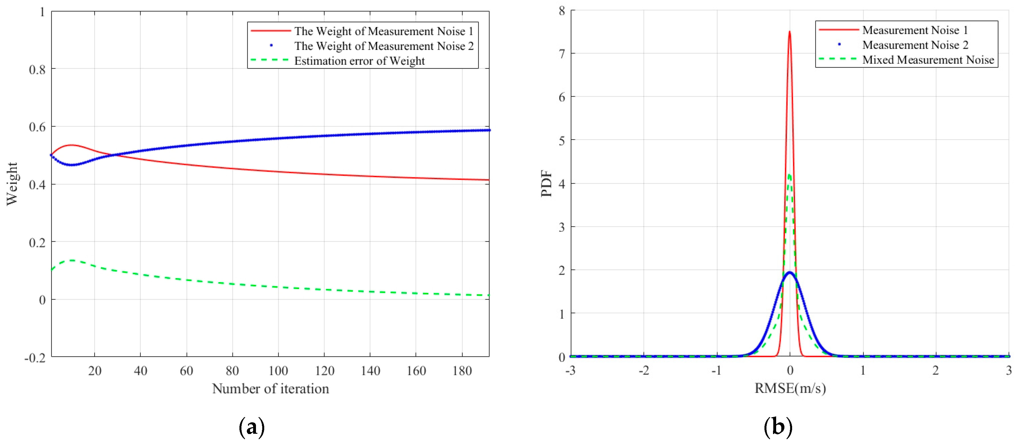
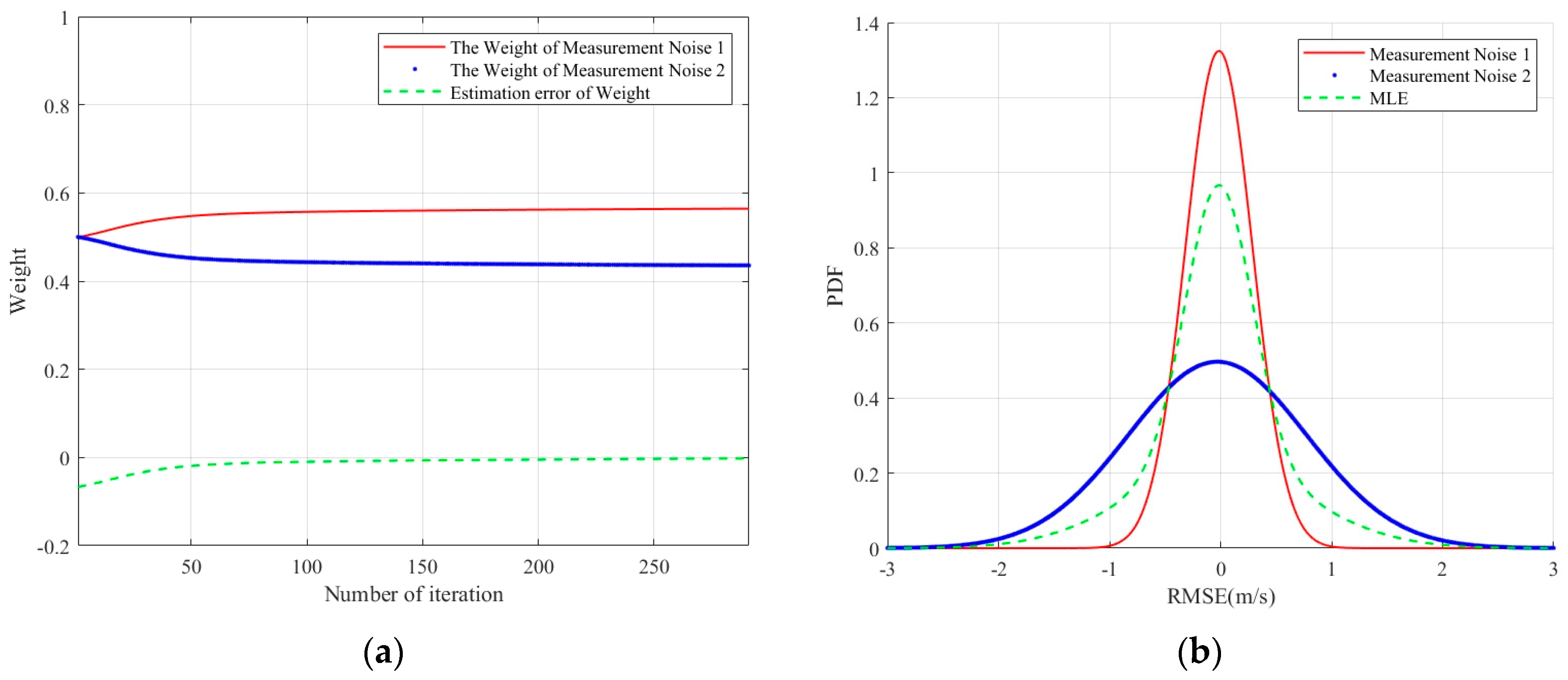
The GNSS velocity error can generally be considered a zero-mean Gaussian distribution. At the same time, after the RTK state GNSS/odometer fusion correction, the odometer scale factor error can be ignored. Therefore, the expected values of the above three residual sequences were set to 0 m/s. According to the empirical value, the initial parameters of the GMM were set, and the above three sets of binary Gaussian distribution data were estimated, respectively. Then, each set of data estimated two sets of corresponding expectations, RMSEs, and their weights, as shown in Figure 5, Figure 6 and Figure 7.
Figure 5, Figure 6 and Figure 7 show the performance of the GMM algorithm in estimating the GNSS measurement noise in the three typical urban complex road environments, as indicated in Table 1. Figure 5a shows the estimation effect of the GMM on the weights of the RTK and SPP measurement data, which gradually converge after 180 iterations. Figure 5b uses curves of three colors to, respectively, display the PDFs of the RTK, SPP, and the hybrid data. The measurement errors of both the RTK and SPP conform to a zero-mean Gaussian distribution. When mixed according to their respective weights, their statistical properties remain as a zero-mean distribution. Figure 6 and Figure 7, respectively, display the estimation of the statistical properties of the two types of hybrid GNSS state measurement data, RTK + CE and SPP + CE, using the GMM algorithm. In using the MLE method, the above three groups of data were estimated, respectively, and each group of data could obtain a set of corresponding expectation and root mean square error parameters. Table 2 shows the MLE algorithm estimation values, GMM algorithm estimation values, and error comparison analysis results of the above three groups of parameters.
As shown in the table, the MLE algorithm estimates the new information sequences of the RTK + SPP, RTK + CE, and SPP + CE mixed navigation modes as a whole, respectively. Therefore, each group of data only corresponds to a set of expectations and RMSEs. Under the “estimation error/true value ratio”, one group of MLE data is represented as “-”. The expectations of the mixed new information sequences were all 0 m/s, so both the MLE and GMM algorithms can achieve accurate expectation estimations. The RMSE parameters of the residual sequences are quite different, and the estimation accuracy of the GMM is significantly higher than that of the MLE, with a maximum improvement of 26.2%. This is mainly because of the MLE estimating two different sequences as the same probability distribution will introduce significant errors that cannot be ignored. Compared to RTK + SPP (21.65%) and SPP + CE (15.09%), in RTK + CE mode, the difference in system accuracy between the two GNSS operating states is the greatest. Therefore, the improvement in the estimation accuracy of the GMM is also more significant.

5.2. Real-World Road Test

The test was conducted in Xiqing District, Tianjin, China. The test equipment is shown in Table 3.
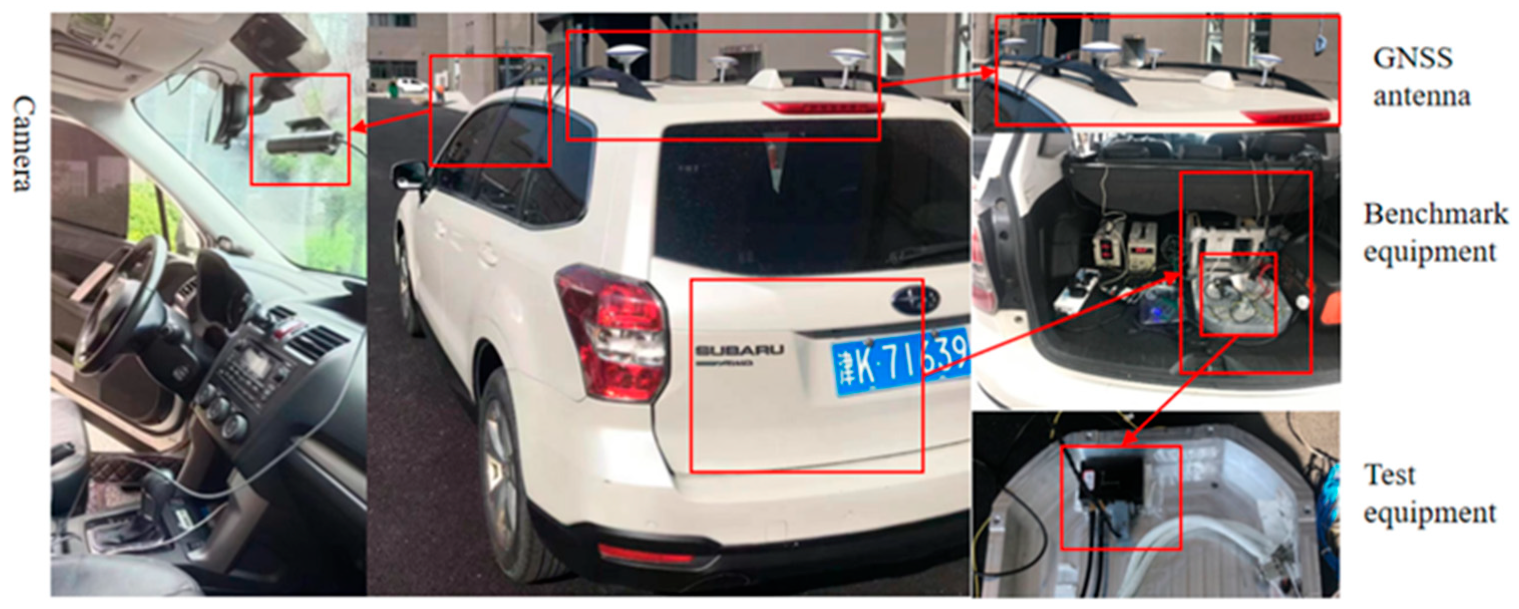
The reference device (TJYJ/15-S1) in Table 3 is a high-precision fiber-optic inertial/satellite system, which provided high-precision reference information for the test. In order to obtain accurate reference information and environmental errors and to compare the algorithm improvement effect more clearly, the test simulated a GNSS single-point positioning and satellite navigation challenging environment (Gaussian noise simulating positioning errors) through software in a specific road section. The specific test method was as follows:
(1) In the whole test section, the reference device collects the fusion positioning data in RTK working mode, which is used as the theoretical reference value;
(2) In the RTK positioning section, the traditional factor graph model and the proposed model are used to solve the data of each sensor subsystem synchronously;
(3) In the GNSS single-point positioning section, GNSS data are collected in non-differential mode, and the data are fused with other sensor subsystems using two model algorithms;
(4) In the GNSS challenging environment section, Gaussian noise is added to the collected GNSS data to simulate the satellite data of a complex urban road environment with multiple interference factors superimposed.
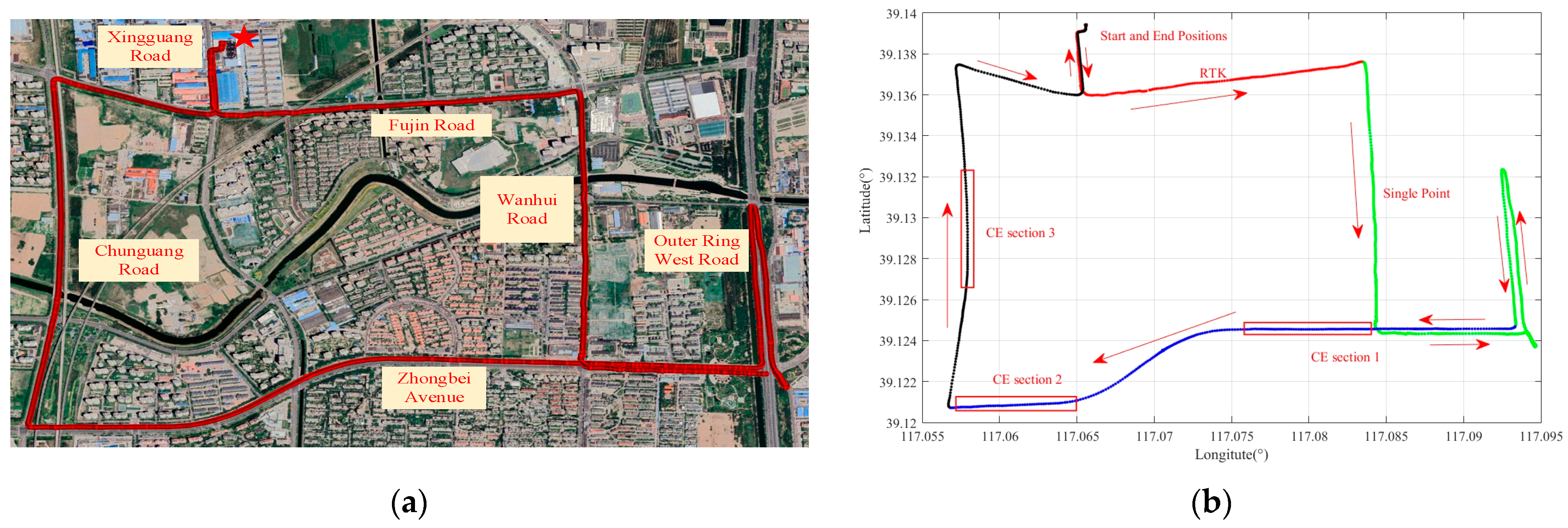
The test route and urban road environment simulation are shown in Figure 8, starting and ending at 27 Xingguang Road, Xiqing District (★ in the figure).
As shown in Figure 8a, the test vehicle traveled southward to Fujin Road, passing Wanhuai Road, Outer Ring West Road, Zhongbei Avenue, Chunhua Road, Fujin Road, and Xingguang Road along the way. The total route length was 12.508 km, and the driving time was 28 min and 57 s. Figure 8b illustrates the driving directions of the test vehicle, the RTK road section, the single-point positioning road section, and the CE road section setting scheme. The test route and test vehicle are shown in Figure 9. The reference equipment and test equipment were fixed using hexahedral tooling and aluminum tooling, respectively, and rigidly connected to each other.
The vehicle’s speed profile during the test is shown in Figure 10. The maximum vehicle speed was 18.5422 m/s (corresponding to 66.75 km/h) at 699 s, with the maximum eastward speed reaching 18.5417 m/s. At 1426 s, the maximum northward speed reached 18.1506 m/s (corresponding to 65.35 km/h). The test vehicle performed various maneuvers during the test, including acceleration, deceleration, stopping, high/low-speed driving, left turns, right turns, and U-turns. The average driving speed was 25.94 km/h.
To validate the performance of the proposed adaptive factor graph with a resilient noise model algorithm, we conducted a comparative analysis with a traditional factor graph approach. Figure 11 presents the speed errors obtained for all test sections.
Figure 11 shows the speed errors obtained for both the AFG and FG algorithms. It can be observed that both algorithms exhibit comparable accuracies under RTK conditions. However, when transitioning to single-point positioning, the AFG algorithm demonstrates the ability to improve in accuracy to a limited extent through the online estimation and correction of the noise model. In challenging satellite navigation environments, the traditional FG algorithm fails to effectively identify external interference, resulting in significant fluctuations in speed error. In contrast, the AFG algorithm not only recognizes the impact of external factors on the system but also accurately estimates them. In adjusting the noise covariance matrix parameters, the influence of environmental factors can be substantially reduced.
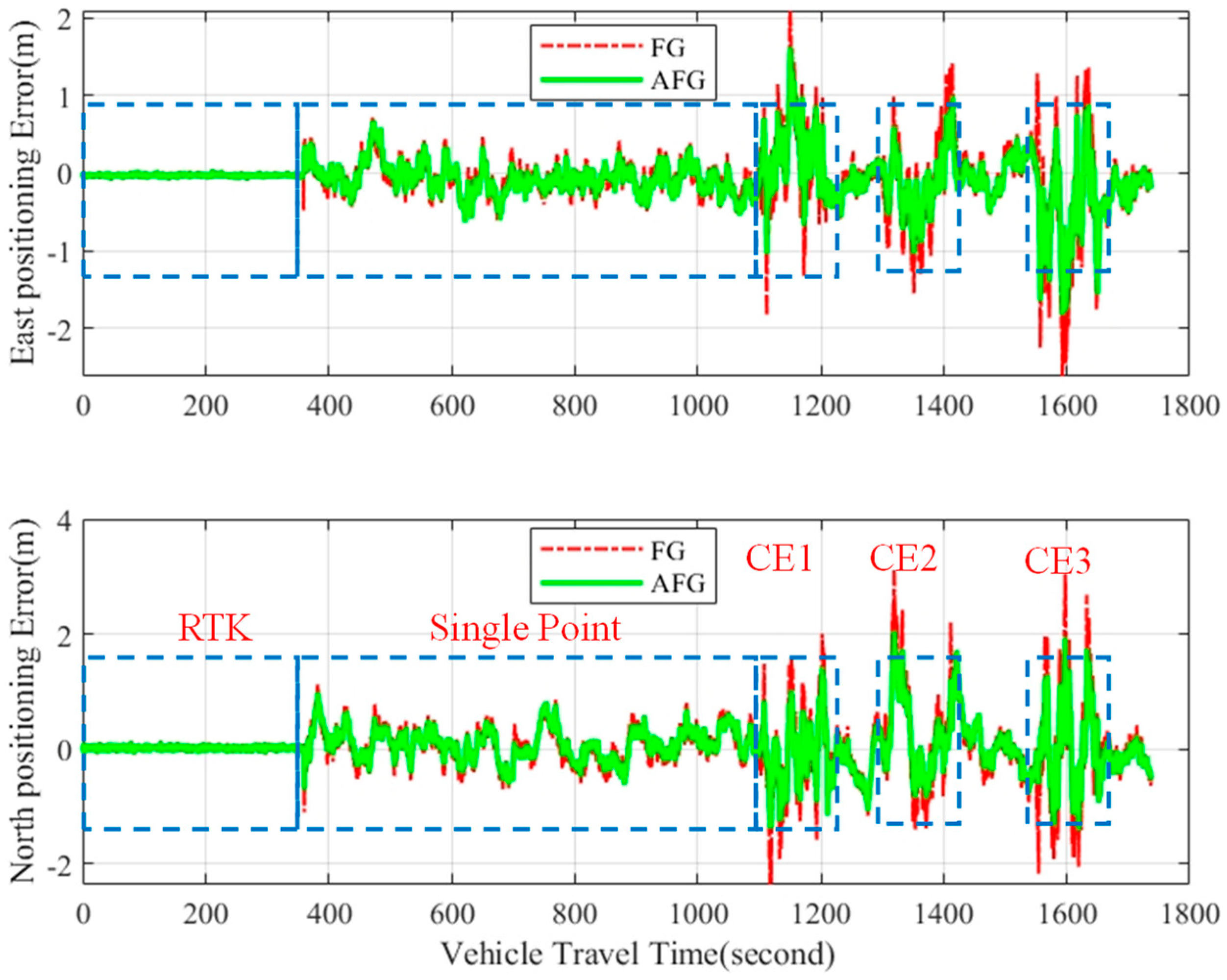
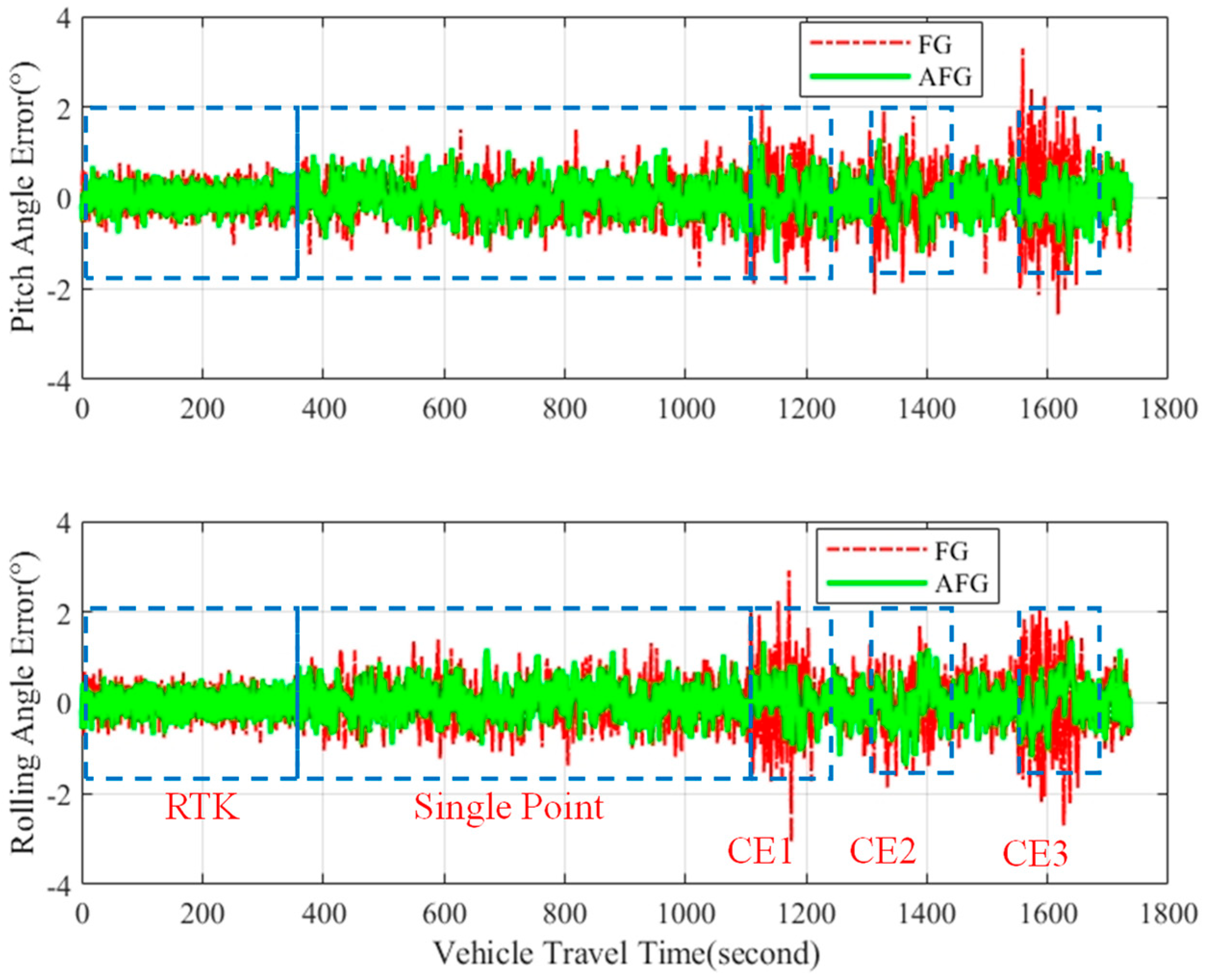
Furthermore, the errors in position, attitude angles, and heading angle obtained by both algorithms exhibit consistency with the speed errors, as shown in Figure 12, Figure 13 and Figure 14.
As shown in Figure 12, the trends of the east and north positioning errors are essentially the same as the velocity error shown in Figure 11. The AGF algorithm has significantly improved the system accuracy through performing an approximate Gaussian estimation of the GNSS measurement noise parameters for the three CE road segments. Figure 13 and Figure 14, respectively, present the attitude and heading errors, from which it can be observed that the improvement in heading error is more significant. This is mainly because autonomous vehicles driving on urban roads have relatively small changes in attitude angles, and the errors are not fully stimulated. To facilitate a more comprehensive analysis of the AFG algorithm’s improvement, the RMSEs from Figure 11, Figure 12, Figure 13 and Figure 14 are statistically summarized in Table 4. Additionally, Table 5 presents the calculated accuracy improvement achieved by the AFG algorithm.
As evidenced in Table 4 and Table 5, the AFG algorithm significantly enhances the accuracy of multi-source integration positioning systems in urban complex road environments compared to the traditional FG algorithm. Notably, in challenging road sections, the heading error is improved by up to 65.63%. This improvement primarily stems from the ability of the AFG algorithm to effectively suppress error divergence through model optimization. In contrast, the FG algorithm’s heading error estimation accuracy is significantly reduced during the low-speed phase of Zhongbei Avenue (CE-1) due to the rapid increase in speed error. Furthermore, in the CE discussed in Section 3, the AGE-FG algorithm achieves accuracy improvements of 27.80%, 32.34%, 39.52%, and 42.95% for speed and position errors. This is mainly attributed to the larger errors introduced in this section, which amplifies the effectiveness of the AFG algorithm’s error estimation improvement. Additionally, the higher speed in the CE discussed in Section 3 reduces the proportion of the speed error in the true value, enhancing the accuracy of the track angle. Consequently, the AFG algorithm’s improvement in heading error estimation accuracy is less pronounced.

6. Conclusions

To address the issues of insufficient continuity and poor accuracy in multi-sensor fusion positioning caused by the GNSS’s vulnerability in urban canyon environments, this paper proposes a resilient factor graph-based fusion positioning algorithm enhanced by the approximate Gaussian estimation of noise models. Firstly, leveraging the autonomy and accuracy advantages of odometry data, GNSS/odometry ground speed residual sequences are used as measurement values for noise parameter estimation, and their approximate Gaussian distribution characteristics are analyzed. Furthermore, based on variational Bayesian networks and Gaussian mixture models, the resilient noise model based on approximate Gaussian estimation is proposed. Finally, the resilient factor graph-based IMU/GNSS/vision/odometer integrated navigation system was tested and verified through simulation platforms and real-vehicle road tests. The results demonstrate the effectiveness and superiority of the algorithm, with heading, speed, and position accuracy improvements of up to 65.63%, 32.34%, and 42.95%, respectively, in GNSS-challenging environments.
Although the above research achieved good results, there are still some limitations that can be improved upon in the future work. From the perspective of optimizing the factor graph multi-sensor data fusion model, dynamically optimizing the sliding window, the online adjustment of feedback correction coefficients, and autonomous sensor fusion are all promising research directions. Firstly, by predicting the positioning state of urban roads based on prior maps and real-time positioning data, the factor graph sliding window size can be resilient and adjusted to improve the system’s positioning accuracy; secondly, the online calculation of the system observability and dynamic optimization of feedback correction coefficients for state estimation values based on this calculation can enhance the system’s fault tolerance and robustness; additionally, combining multi-sensor fusion global positioning with LiDAR local positioning can significantly improve the integrity and safety of autonomous vehicle driving. The use of artificial intelligence technology for the auxiliary optimization of multi-sensor autonomous fusion navigation systems is also an important research direction. Firstly, in using a visual foundation model to intelligently recognize the road environment, GNSS measurement noise estimations can be obtained, and then the online adaptive optimization of the data fusion model can be achieved; secondly, based on deep learning neural networks and prior maps, the optimal estimation of the observability of the data fusion model can greatly improve the robustness and fault tolerance of the system.

Author Contributions

Conceptualization and methodology, Z.L. and Q.M.; software, writing—original draft preparation, and validation, Z.L.; investigation and data curation, Z.S. and H.J.; visualization, L.W. and L.L.; writing—review and editing, supervision, project administration, and funding acquisition, Q.M. All authors have read and agreed to the published version of the manuscript.

Funding

This work was funded by the National Natural Science Foundation of China (No. 62388101 and No. 62203111), Aeronautical Science Foundation of China (20220008069003), Natural Science Foundation of Jiangsu Province (No. BK20231434), and Jiangsu Provincial Department of Science and Technology (No. BM2023013).

Data Availability Statement

The datasets used and/or analyzed during the current study are available from the corresponding author upon reasonable request.

Conflicts of Interest

Author Ziyue Li was employed by the company Beijing Kunpeng Borui Technology. The remaining authors declare that the research was conducted in the absence of any commercial or financial relationships that could be construed as a potential conflict of interest.

References

  1. Ali, A.; Chan, B.; Omr, M.; Georgy, J. Coursa Drive: Integrated Navigation Solution for Autonomous Vehicles. In Proceedings of the 32nd International Technical Meeting of the Satellite Division of The Institute of Navigation (ION GNSS+ 2019), Miami, FL, USA, 16–20 September 2019; pp. 1220–1233. [Google Scholar]
  2. Woo, A.; Baris, F.; Melek, W.W. Localization for autonomous driving. In Handbook of Position Location: Theory, Practice, and Advances, 2nd ed.; Wiley: Hoboken, NJ, USA, 2018; pp. 1051–1087. [Google Scholar]
  3. Chiang, K.W.; Chiu, Y.T.; Srinara, S.; Tsai, M. Performance of LiDAR-SLAM-based PNT with initial poses based on NDT scan matching algorithm. Satell. Navig. 2023, 4, 3. [Google Scholar] [CrossRef]
  4. Vivacqua, R.P.D.; Bertozzi, M.; Cerri, P.; Martins, F.N.; Vassallo, R.F. Self-localization based on visual lane marking maps: An accurate low-cost approach for autonomous driving. IEEE Trans. Intell. Transp. Syst. 2017, 19, 582–597. [Google Scholar] [CrossRef]
  5. Liu, W.; Wu, M.; Zhang, X.; Wang, W.; Ke, W.; Zhu, Z. Single-epoch RTK performance assessment of tightly combined BDS-2 and newly complete BDS-3. Satell. Navig. 2021, 2, 6. [Google Scholar] [CrossRef]
  6. Wang, Z.; Wu, Y.; Niu, Q. Multi-sensor fusion in automated driving: A survey. IEEE Access 2019, 8, 2847–2868. [Google Scholar] [CrossRef]
  7. Fayyad, J.; Jaradat, M.A.; Gruyer, D.; Najjaran, H. Deep Learning Sensor Fusion for Autonomous Vehicle Perception and Localization: A Review. Sensors 2020, 20, 4220. [Google Scholar] [CrossRef]
  8. Li, Q.; Queralta, J.P.; Gia, T.N.; Zou, Z.; Westerlund, T. Multi-sensor fusion for navigation and mapping in autonomous vehicles: Accurate localization in urban environments. Unmanned Syst. 2020, 8, 229–237. [Google Scholar] [CrossRef]
  9. Li, A.; Zhang, Y.; Ji, Y.; Guo, Y.; Zhang, Z. An Post-processing Method of Enhancing Position Accuracy of Strapdown Inertial/Odometer System. Navig. Position. Timing 2021, 8, 75–80. [Google Scholar]
  10. Li, Z.; Liu, Y.; Zeng, Q.; Liu, J.; Li, F.; Zhang, G. A Vision/Map Attitude Matrix Aided IMU/Odometer Integrated Navigation Method. In Proceedings of the 2022 IEEE International Conference on Unmanned Systems (ICUS), Guangzhou, China, 28–30 October 2022; pp. 254–259. [Google Scholar]
  11. Rahman, M.T.; Karamat, T.; Givigi, S.; Noureldin, A. Improving multisensor positioning of land vehicles with integrated visual odometry for next-generation self-driving cars. J. Adv. Transp. 2018, 2018, 6513970. [Google Scholar] [CrossRef]
  12. Meng, Q.; Hsu, L.T. Resilient interactive sensor-independent-update fusion navigation method. IEEE Trans. Intell. Transp. Syst. 2022, 23, 16433–16447. [Google Scholar] [CrossRef]
  13. Li, X.; Wang, X.; Liao, J.; Li, X.; Li, S.; Lyu, H. Semi-tightly coupled integration of multi-GNSS PPP and S-VINS for precise positioning in GNSS-challenged environments. Satell. Navig. 2021, 2, 1. [Google Scholar] [CrossRef]
  14. Rosique, F.; Navarro, P.J.; Fernández, C.; Padilla, A. A Systematic Review of Perception System and Simulators for Autonomous Vehicles Research. Sensors 2019, 19, 648. [Google Scholar] [CrossRef] [PubMed]
  15. Yang, Y. Resilient PNT concept frame. J. Geod. Geoinf. Sci. 2019, 2, 1–7. [Google Scholar]
  16. Huang, K.; Shi, B.; Li, X.; Li, X.; Huang, S.; Li, Y. Multi-modal sensor fusion for auto driving perception: A survey. arXiv 2022, arXiv:2202.02703. [Google Scholar]
  17. Aftatah, M.; Lahrech, A.; Abounada, A.; Soulhi, A. GPS/INS/Odometer data fusion for land vehicle localization in GPS denied environment. Mod. Appl. Sci. 2016, 11, 62. [Google Scholar] [CrossRef]
  18. Meng, Q.; Hsu, L.T. Integrity Monitoring for All-Source Navigation Enhanced by Kalman Filter based Solution Separation. IEEE Sens. J. 2021, 21, 15469–15484. [Google Scholar] [CrossRef]
  19. Kschischang, F.R.; Frey, B.J.; Loeliger, H.A. Factor graphs and the sum-product algorithm. IEEE Trans. Inf. Theory 2001, 47, 498–519. [Google Scholar] [CrossRef]
  20. Zeng, Q.; Chen, W.; Liu, J.; Wang, H. An Improved Multi-Sensor Fusion Navigation Algorithm Based on the Factor Graph. Sensors 2017, 17, 641. [Google Scholar] [CrossRef] [PubMed]
  21. Wen, W.; Kan, Y.C.; Hsu, L.-T. Performance Comparison of GNSS/INS Integrations Based on EKF and Factor Graph Optimization. In Proceedings of the 32nd International Technical Meeting of the Satellite Division of The Institute of Navigation (ION GNSS+ 2019), Miami, FL, USA, 16–20 September 2019; pp. 3019–3032. [Google Scholar] [CrossRef]
  22. Wen, W.; Pfeifer, T.; Bai, X.; Hsu, L.T. It is time for Factor Graph Optimization for GNSS/INS Integration: Comparison between FGO and EKF. arXiv 2004, arXiv:2004.10572. [Google Scholar]
  23. Zhao, S.; Chen, Y.; Farrell, J.A. High-precision vehicle navigation in urban environments using an MEM’s IMU and single-frequency GPS receiver. IEEE Trans. Intell. Transp. Syst. 2016, 17, 2854–2867. [Google Scholar] [CrossRef]
  24. Gao, J.; Tang, X.; Zhang, H.; Wu, M. Vehicle INS/GNSS/OD integrated navigation algorithm based on factor graph. Syst. Eng. Electron. 2018, 40, 2547–2553. [Google Scholar] [CrossRef]
  25. Li, W.; Cui, X.; Lu, M. A robust graph optimization realization of tightly coupled GNSS/INS integrated navigation system for urban vehicles. Tsinghua Sci. Technol. 2018, 23, 724–732. [Google Scholar] [CrossRef]
  26. Sarkka, S.; Nummenmaa, A. Recursive noise adaptive Kalman filtering by variational Bayesian approximations. IEEE Trans. Autom. Control 2009, 54, 596–600. [Google Scholar] [CrossRef]
  27. Li, K.; Chang, L.; Hu, B. A variational Bayesian-based unscented Kalman filter with both adaptivity and robustness. IEEE Sens. J. 2016, 16, 6966–6976. [Google Scholar] [CrossRef]
  28. Hu, M.M.; Jing, Z.L.; Peng, D.D.; Zhou, G.R.; Zheng, Z.M. Variational Bayesian filtering based on Student-t distribution for SINS/GPS integrated navigation. J. ZheJiang Univ. 2018, 52, 1482–1488. [Google Scholar]
  29. Liu, Y.; Fan, X.; Lv, C.; Wu, J.; Li, L.; Ding, D. An innovative information fusion method with adaptive Kalman filter for integrated INS/GPS navigation of autonomous vehicles. Mech. Syst. Signal Process. 2018, 100, 605–616. [Google Scholar] [CrossRef]
  30. Yue, Z.; Lian, B.; Tang, C. A GPS/INS Integrated Navigation Method Based on Weighting Adaptive Square-root Cubature Kalman Filter. J. Electron. Inf. Technol. 2018, 40, 565–572. [Google Scholar] [CrossRef]
  31. Xu, H.; Lian, B.; Liu, S. Multi-source integrated navigation algorithm for iterated maximum posteriori estimation based on sliding-window factor graph. Acta Armamentarii 2019, 40, 807. [Google Scholar]
  32. Jing, C.; Huang, G.; Li, X.; Zhang, Q.; Yang, H.; Zhang, K.; Liu, G. GNSS/accelerometer integrated deformation monitoring algorithm based on sensors adaptive noise modeling. Measurement 2023, 218, 113179. [Google Scholar] [CrossRef]
  33. Watson, R.M.; Gross, J.N.; Taylor, C.N.; Leishman, R.C. Uncertainty Model Estimation in an Augmented Data Space for Robust State Estimation. In Proceedings of the 33rd International Technical Meeting of the Satellite Division of The Institute of Navigation (ION GNSS+ 2020), Online, 21–25 September 2020; pp. 2686–2695. [Google Scholar] [CrossRef]
  34. Li, Z.; Zeng, Q.; Liu, Y.; Liu, J. An ROI Optimization Method Based on Dynamic Estimation Adjustment Model. Remote Sens. 2023, 15, 2434. [Google Scholar] [CrossRef]
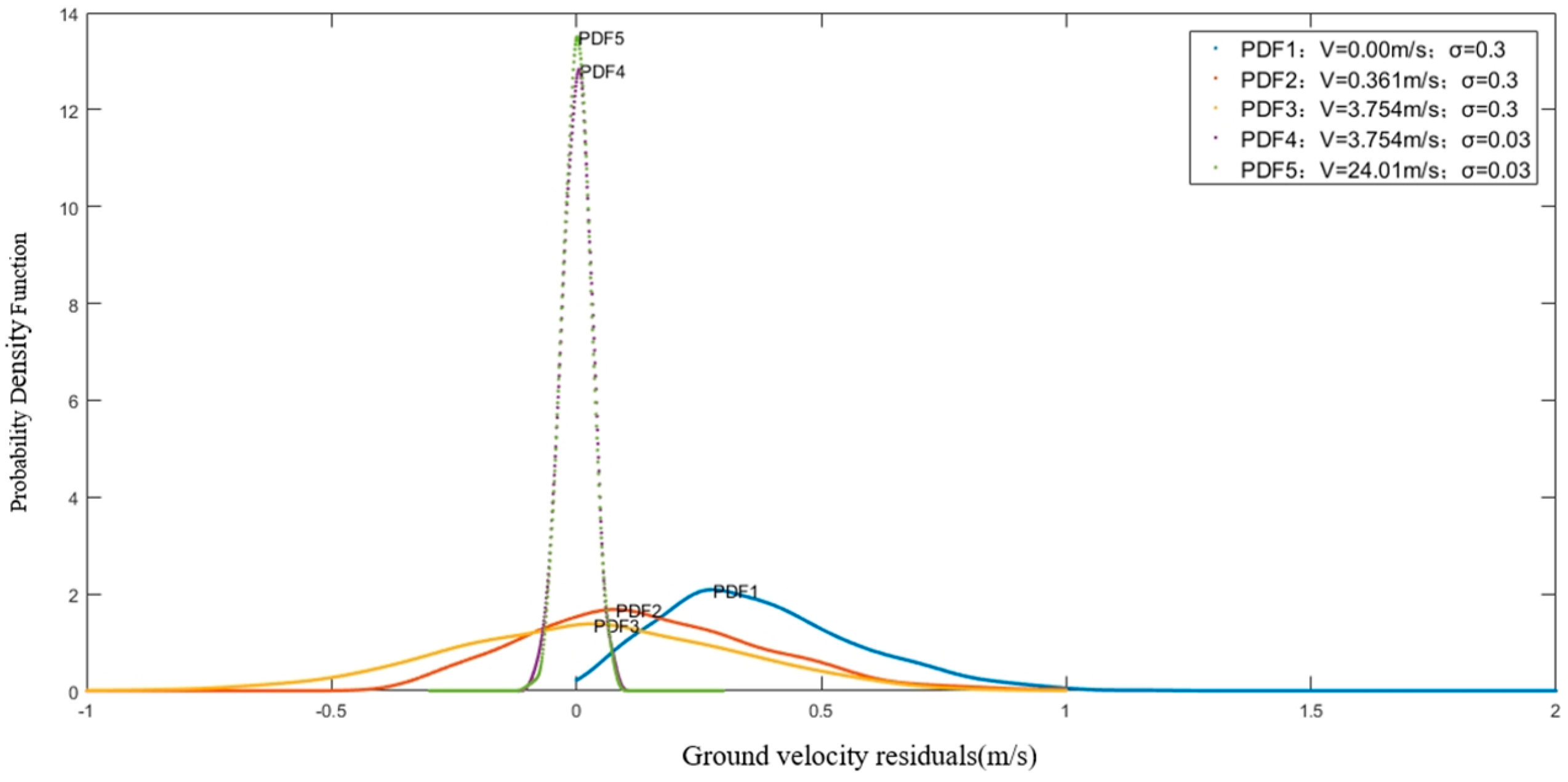
Figure 1. The residual sequence distribution characteristics.
Remotesensing 16 02176 g001
Figure 2. The noise variance curve and the segmentation of the approximate Gaussian fitting region (AGFR) and approximate Gaussian convergence region (AGCR).
Remotesensing 16 02176 g002
Figure 3. Multi-sensor fusion localization algorithm based on GMM noise parameter estimation.
Remotesensing 16 02176 g003
Figure 4. Architecture diagram of multi-sensor fusion positioning system based on adaptive factor graph.
Remotesensing 16 02176 g004
Figure 5. Estimation results of the GMM algorithm for the residual sequence in the RTK/SPP mixed scenario. (a) The weight estimation error of the measurement noise sequence; (b) the probability density function for measuring noise sequences.
Remotesensing 16 02176 g005
Figure 6. Estimation results of the GMM algorithm for the residual sequence in the RTK/CE mixed scenario. (a) The weight estimation error of the measurement noise sequence; (b) the probability density function for measuring noise sequences.
Remotesensing 16 02176 g006
Figure 7. Estimation results of the GMM algorithm for the residual sequence in the SPP/CE mixed scenario. (a) The weight estimation error of the measurement noise sequence; (b) the probability density function for measuring noise sequences.
Remotesensing 16 02176 g007
Figure 8. Adaptive factor graph fusion localization algorithm for vehicle test route planning based on approximate Gaussian estimation. (a) On-road vehicle test route planning; (b) urban road environment simulation scheme.
Remotesensing 16 02176 g008
Figure 9. Adaptive factor graph fusion localization algorithm for vehicle test route planning based on approximate Gaussian estimation: on-road vehicle test with real-world data.
Remotesensing 16 02176 g009
Figure 10. Urban road test, vehicle speed profile.
Remotesensing 16 02176 g010
Figure 11. Real-world driving test, speed error comparison plot.
Remotesensing 16 02176 g011
Figure 12. Real-world driving test, position error comparison plot.
Remotesensing 16 02176 g012
Figure 13. Real-world driving test, attitude angle error comparison plot.
Remotesensing 16 02176 g013
Figure 14. Real-world driving test, heading angle error comparison plot.
Remotesensing 16 02176 g014
Table 1. Simulation parameter table for innovation sequence.
Mixed Positioning StateRTKSPPRTKCESPPCE
ParameterMean0.00000.00000.00000.00000.00000.0000
RMSE0.05000.20000.06000.60000.30000.8000
weight0.40000.60000.46670.53330.33330.6667
Table 2. Estimation and comparison of MLE and GMM algorithms.
Positioning StateMLE Estimated ValueGMM Estimated ValueEstimation Error/Truth Value Ratio
MeanRMSEMeanRMSEWeightMLEGMMImprovement
RTK
SPP
0.00550.1560−0.00180.05390.4153-7.80%-
−0.00390.19930.584722%0.35%21.65% ↑
RTK
CE
−0.00440.4418−0.00410.06310.4625-5.17%-
0.00240.05900.537526.37%0.17%26.2% ↑
SPP
CE
−0.00120.66650.01080.28380.3354-5.40%-
−0.00230.78790.674616.60%1.51%15.09% ↑
Table 3. Test equipment and parameter list.
DeviceManufacturer/ModelMain ParametersInterface
Reference equipmentSPATIOTEMPORAL/TJYJ/15-S1Gyroscope, 0.01°/h; Attitude, 0.03°; Heading, 0.05°RS422
GNSSSPATIOTEM-PORAL/SKJW-09RTK, 2 cm + 1 ppm (CEP); Speed, 0.05 m/s; Attitude, 0.2°RS422
INSSPATIOTEM-PORAL/SKJW-09Gyroscope, 30°/h; Accelerometer, 1 mgRS422
Wheel speed encoderKubler/Sendix7058Maximum speed, 600 r/min; Resolution 16 bit, 1~65,535CAN
StereovisionSmarter Eye/SE1Depth of detection, 2~60 m; Baseline, 12 cm; Picture frame rate, 25 fps; HFOV, 40°; Pitch angle, 70~90°CAN
Domain controllerAixun Hongda/6388H-ZS4 generation I7 Celeron processor; 16 G of memory; 512 G solid-state drivemulti-interface
Table 4. Comparison of navigation accuracy between FG and proposed AFG algorithm.
ParameterRTKSPPCE-1CE-2CE-3
FGAFGFGAFGFGAFGFGAFGFGAFG
δ θ (°)0.22820.21650.42040.35510.75310.35740.54460.46320.83660.5264
δ γ (°)0.22590.21890.41510.32850.60690.53270.58450.62720.93150.6569
δ φ (°)0.21790.20780.96420.98535.16041.77363.81251.09951.50661.4190
δ v E (m/s)0.01780.01730.07200.06880.20590.16370.17130.15610.28190.1790
δ v N (m/s)0.01710.01690.07330.06890.22530.16110.16860.13970.31110.2105
δ p E (m)0.01780.01730.21190.19780.67210.50020.47450.35070.71500.4324
δ p N (m)0.03070.02860.28570.24420.87780.58490.69590.43841.40270.8003
Table 5. Statistical summary of accuracy improvement achieved by AFG algorithm compared to FG.
ParameterRTKSPPCE-1CE-2CE-3
δ θ (°)5.13%8.40%47.23%16.78%37.08%
δ γ (°)3.10%13.97%23.76%13.22%29.48%
δ φ (°)4.64%2.19%65.63%60.91%19.08%
δ v E (m/s)2.81%4.44%20.50%14.71%27.80%
δ v N (m/s)1.17%6.00%28.50%17.14%32.34%
δ p E (m)2.81%6.65%25.58%26.09%39.52%
δ p N (m)6.84%14.53%33.37%37.00%42.95%
Disclaimer/Publisher’s Note: The statements, opinions and data contained in all publications are solely those of the individual author(s) and contributor(s) and not of MDPI and/or the editor(s). MDPI and/or the editor(s) disclaim responsibility for any injury to people or property resulting from any ideas, methods, instructions or products referred to in the content.