Article

Hyperspectral Estimation of Chlorophyll Content in Grape Leaves Based on Fractional-Order Differentiation and Random Forest Algorithm

1
School of Agricultural Engineering, Jiangsu University, Zhenjiang 212013, China
2
Key Laboratory of Quantitative Remote Sensing in Ministry of Agriculture and Rural Affairs, Information Technology Research Center, Beijing Academy of Agricultural and Forestry Sciences, Beijing 100097, China
*
Author to whom correspondence should be addressed.
Remote Sens. 2024, 16(12), 2174; https://doi.org/10.3390/rs16122174
Submission received: 26 April 2024 / Revised: 10 June 2024 / Accepted: 13 June 2024 / Published: 15 June 2024

Abstract

:
Chlorophyll, as a key component of crop leaves for photosynthesis, is one significant indicator for evaluating the photosynthetic efficiency and developmental status of crops. Fractional-order differentiation (FOD) enhances the feature spectral information and reduces the background noise. In this study, we analyzed hyperspectral data from grape leaves of different varieties and fertility periods with FOD to monitor the leaves’ chlorophyll content (LCC). Firstly, through sensitive analysis, the fractional-order differential character bands were identified, which was used to construct the typical vegetation index (VI). Then, the grape LCC prediction model was built based on the random forest regression algorithm (RFR). The results showed the following: (1) FOD differential spectra had a higher sensitivity to LCC compared with the original spectra, and the constructed VIs had the best estimation performance at the 1.2th-order differential. (2) The accuracy of the FOD-RFR model was better than that of the conventional integer-order model at different fertility periods, but there were differences in the number of optimal orders. (3) The LCC prediction model for whole fertility periods achieved good prediction at order 1.3, R 2 = 0.778, RMSE = 2.1, and NRMSE = 4.7%. As compared to the original reflectance spectra, R2 improved by 0.173; RMSE and NRMSE decreased, respectively, by 0.699 and 1.5%. This indicates that the combination of FOD and RFR based on hyperspectral data has great potential for the efficient monitoring of grape LCC. It can provide technical support for the rapid quantitative estimation of grape LCC and methodological reference for other physiological and biochemical indicators in hyperspectral monitoring.

1. Introduction

The chlorophyll level affects the photosynthetic capacity of grapes, which can provide nutrients for fruit coloring, the tree’s growth, germination and differentiation. It is an important indicator of the growth of grapes from fruiting to ripening [1,2]. If the leaf chlorophyll content (LCC) is too low, leaf senescence will directly affect the synthesis of organic nutrients, resulting in grapes not coloring or once-fully colored grapes showing soft fruit and drop grains, which directly affects the quality of the fruit [3]. Therefore, an accurate assessment of LCC can help to determine fertilization and canopy management strategies within the framework of precision viticulture, thus improving vine and fruit growth [4,5].
Traditional methods for chlorophyll content determination are complex, which leads to longer time consumption and damage to the leaves [6]. Handheld portable chlorophyll meters can determine relative chlorophyll content, but only measure individual leaves point by point, which is a large amount of work and does not allow for the real-time monitoring of plant variables [7]. Therefore, a rapid, inexpensive, and accurate method is needed to assess crop chlorophyll content. In recent years, hyperspectral remote sensing technology has been developing rapidly: hyperspectral equipment provides a fast, non-destructive, and timely method of data collection, which can be used to measure the nutrient status of crops and to determine the growth of plants [8]. Scholars have conducted in-depth studies on the hyperspectral remote sensing of vegetation, including estimation of biomass [9], nitrogen content [10], water content [11], and leaf area index [12].
The spectral reflectance characteristics of green plants are determined by their chemical and morphological features, which are closely related to the development and health of the vegetation as well as to the growing conditions. In the visible wavelength band, chlorophyll is the main factor governing the spectral response of plants [13]. More and more scholars are focusing on the spectral characteristics of vegetation leaves at different chlorophyll levels [14,15] in the hope of realizing fast, nondestructive, and real-time LCC monitoring. Zhao et al. [16] analyzed the trends of LCC and the spectral response of maize at each reproductive stage, extracted LCC-sensitive features such as reflectance intensity and wavelength change position, and established an LCC detection model by partial least squares (PLS) regression. Li et al. [17] utilized canopy spectral reflectance and its first-order derivatives to develop new spectral parameters based on the red-edge region and establish a quantitative detection model to estimate winter oilseed rape chlorophyll density. In addition, combinations of methods such as integrated vegetation indices [18], machine learning algorithms [19], and spectral mathematical variations [20] have been widely used in the search for chlorophyll-sensitive metrics and the construction of monitoring models.
The preprocessing of hyperspectral data is crucial for the establishment of high-precision inversion models. Appropriate preprocessing methods can make full use of the spectrally valid information and highlight the spectral features while reducing the noise to improve the inversion accuracy of the prediction models [21,22]. Existing studies mostly utilize conventional integer-order derivatives [23,24] as a hyperspectral preprocessing method to determine the information about the characteristic wavelength positions of the maximum, minimum, and inflection reflectance of hyperspectral reflectance curves. However, integer-order differential derivative spectra tend to ignore the asymptotic information in the spectrum due to the large difference; some useful data information will be discarded during processing [25,26]. Fractional-order differentiation (FOD) was proposed by Gottfried Wilhelm Leibniz and can process spectra in smaller difference steps [27]. With the advantages of “memory” and “global”, FOD can eliminate background noise, amplify detailed information, and remove baseline drift, which is widely used in spectral preprocessing [28,29]. Ren et al. [30] screened sensitive features such as FOD based on CC and predictor variable importance (VIP), and accepted and imported them into different machine-learning models for prediction of stripe rust in winter wheat through collaboration among the features, and found the method works well for high-precision surveillance. Abulaiti et al. [31] explored the effect of FOD on cotton canopy spectra and analyzed the correlation between the total nitrogen content (TNC) and FOD spectra of cotton by Pearson correlation and comparison of optimized spectral indices, based on the Support Vector Machine (SVM) regression model to construct a model for estimating TNC in cotton. All the above studies show that FOD can describe the physical properties of the system more clearly, reveal the essential characteristics of the research object, and be more accurate in describing the system model than the integer-order derivatives.
The subtle changes in the crop’s response to the quality, light, duration and direction of light in the growing environment, which in turn causes changes in the physiological and morphological structures necessary for survival in that environment, result in significant differences in the crop spectra of the two regions. In this study, it is proposed to use FOD to analyze the hyperspectral features of grape leaves from the berry growing period to the harvesting period, and analyze the data to determine the sensitive order differential spectral features. By exploring the optimal order for different reproductive periods and constructing a stabilization model for LCC monitoring in grapes, it provides highly efficient technical support for the rapid detection of grape nutrient indexes. The specific contributions of this study are as follows:
(1)
By comparing the LCC hyperspectral response curves of grapes from different periods and species, the reasons for localized differences in the curves were resolved.
(2)
The raw spectra were processed by FOD at 0.1-order intervals to obtain 0.1–2.0-order differential spectral curves. From the perspective of spectral characterization, it was initially concluded that FOD could better handle hyperspectral data.
(3)
We solved the correlation between different orders of spectra and LCC, and screened the characteristic bands to construct vegetation indices for subsequent analysis and modeling.
(4)
Using the screened typical vegetation indices as input features, the RFR method was utilized to establish LCC prediction models for grapes in different periods. Three periods were also validated uniformly to analyze whether there is universality for different fertility period FOD enhancing the model effect.

2. Materials and Methods

2.1. Study Site

As shown in Figure 1, the wine grape Cabernet Sauvignon experimental area was located in Bolongbao Vineyard, Fangshan District, Beijing, which is situated between longitude 131.45–132.2°E and latitude 46.47–47.0°N. The Edible Grape Sunshine Rose Experimental Area was located at Dongfanghong Farm, Yuanmou County, Chuxiong Yi Autonomous Prefecture, Yunnan Province, which is situated at a longitude of 25.75 °E and a latitude of 101.77°N. Sunny Rose grape leaves are fan-shaped, large, and medium–thick in size, with serrated margins and downy undersides. Cabernet Sauvignon grape leaves are small and heart-shaped, with serrated edges, and have five deep lines on them. Since the cultivation centers and the leaves are highly variable, these two types of varieties were selected for this study to find the generalizability of the modeling. The location, time, variety, growing period, and number of plots of grapes collected for the experiment are shown in Table 1.

2.2. Data Acquisition

Data collected in this study included leaf hyperspectral and SPAD values. Four of the most photosynthetically active grapevine “inverted trifoliate leaves” were selected from each plot, and the spectral reflectance of the test samples was measured using an American ASD Filed Spec Pro 2500 back-mounted field spectrometer. Spectral bands are detected in the range of 350–2500 nm, with band accuracy and spectral resolution adjusted to 1 nm. Spectral measurements were made using the instrument’s built-in light source, with the leaf to be measured flat under the spectral detector, which was calibrated with a diffuse reference plate before each measurement of the spectral reflectance of the leaf. For measurement, each leaf was segmented from petiole to tip (avoiding the veins) four times, and 10 spectral reflectance values were collected each time. The SPAD-502plus (Konica Minolta, Tokyo, Japan) chlorophyll content meter was also used to clip the leaves of the test samples for the determination of chlorophyll SPAD values, and the collection points were located at three random sites avoiding the leaf veins. The average value was taken as the final spectral reflectance and chlorophyll content of this sample.

2.3. Hyperspectral Data Processing

The spectroscopic instrument used in this study has a measurement range of 350–2500 nm, with large amounts of hyperspectral data volumes and spectral wavelengths, in addition to large correlations and multiple covariances between neighboring bands [32]. Therefore, the collected spectral data need to be filtered to retain valid information and minimize spectral redundancy to optimize the models. The results of previous studies showed that the chlorophyll-sensitive band is located in the visible and near-infrared wavelength range [24], so 400–1000 nm was intercepted as the range of the research band. The data were then resampled at 1 nm intervals and the original 2151 bands were reduced to 601 bands for subsequent data processing and analysis.
Traditional integer-order differentiation only considers the first- or second-order derivative processing of hyperspectral data, which ignores the spectral asymptotic information and affects the model accuracy. FOD extends the concept of integer-order derivatives. Geometrically, the integer-order derivative is an arbitrary order slope of a function curve, which has the physical meaning of fractional flow and generalized amplitude. It can refine the information of spectral data and effectively denoise and improve the modeling accuracy [33,34]. The more commonly used fractional-order differentials are defined in the form of Grunwald–Letnikov, Riemann–Liouvile, and Caputo [35].
The numerical solution obtained by Grunwald–Letnikov (G-L) is closer to its exact solution due to the difference in the accuracy of the function-solving methods [36]. Therefore, in this paper, we used this method to differentiate the spectral reflectance of grape leaves from 0 to 2 orders, with a step size of 0.1. Fractional-order derivatives of type G-L generalize the integer-order range to fractional-order and are obtained by taking the differential approximation of the original integer-order derivative to the limit of the recursive formula. The G-L definition of the nth-order derivative of a function f ( t ) is:
D t v t 0 G L = lim h 0 1 h v j = 0 t t 0 h ( 1 ) m Γ ( v + 1 ) Γ ( m + 1 ) Γ ( v m + 1 ) · f ( t j h )
Γ α = 0 e x x α 1 d x = α 1 !
The simplification leads to:
d v f ( t ) d t v = f t + v f t 1 + v v + 1 2 ! f t 2 + + Γ ( v + 1 ) m ! Γ ( v n + 1 ) f ( t n )
where t—wavelength, f ( t ) —spectrum, v—arbitrary order, Γ —Gamma function, n —difference between upper and lower differential limits. When v = 0, 1, and 2, they, respectively denote the original spectrum, the first-order differential spectrum, and the second-order differential spectrum.
As can be seen from the formula, the traditional integer-order derivative describes the instantaneous rate of change of the function at a point, and is only relevant to information about points within the differential window. While the fractional-order differentiation generalizes this concept by relating to the points within the window and all previous points, the value of fractional-order differentiation of a certain band at order v is related not only to the hyperspectral reflectance f ( t ) of the current band, but also to f ( t 1 ) , f ( t 2 ) ,…, f ( t n ) . The value of the nth-order FOD is the result of multiplying these time nodes by Γ v + 1 m ! Γ v n + 1 and adding them together. The points that are closer to the current wave are given more weight and have a greater influence on the value of the vth order fractional-order differentiation, which is why fractional-order differentiation exhibits “memorability” and “non-localization” [37]. It also shows that the integer order cannot capture the long-term memory effect of the signal well when processing the signal, while FOD can clearly describe the physical properties of the system and truly reveal the essential characteristics of the research object [38].

2.4. Models and Evaluation Indicators

2.4.1. Principles of Random Forest Regression Modeling

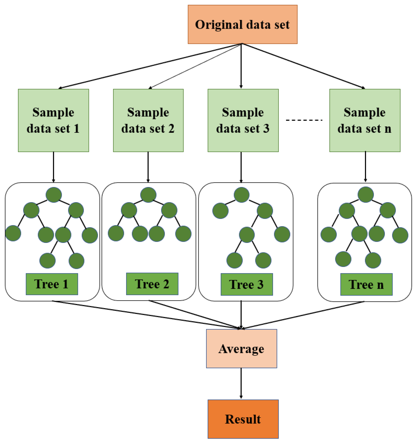
RFR is an important branch of Random Forest. The model builds multiple unrelated decision trees by randomly selecting samples and features, and obtains predictions through a parallel approach. Each decision tree produces a prediction from the extracted samples and features, which can effectively reduce the risk of overfitting. The regression prediction results for the whole forest are obtained by averaging the results of all the trees combined. Algorithmic data are used in scenarios with low dimensionality requirements and high accuracy requirements [39].
Figure 2 represents the regression principle of the algorithm. First, the dataset for training and testing the model needs to be prepared. The dataset contains features and corresponding target variables. Characteristics are the properties used to predict the target variable (VI), while the target variable is the value to be predicted by regression (SPAD). The training set is used to train the model and the test set is used to evaluate the performance of the model. The model will construct multiple decision trees based on the samples in the training set and the values of the target variables, and perform feature selection and segmentation on each tree. The samples in the test set are predicted by the trained RFR. The model will average the prediction results of each decision tree to obtain the final regression prediction results. The performance of the model is evaluated by comparing it with the real target variables [40,41].
RFR is a black-box model and it is difficult to explain its internal decision-making process. However, through the ranking of feature importance, the degree of contribution of different features to the prediction results can be understood, thus explaining the prediction results of the model and making the model interpretable [42]. RFR obtains the final result by averaging the prediction results for each tree. While the fractional-order differential spectra have a higher correlation level between vegetation indices and chlorophyll than those constructed in integer order. This means that the method will improve the prediction accuracy for each tree and hence for the whole forest. Therefore, it is feasible to predict LCC by combining FOD with RFR.

2.4.2. Used Metrics

The coefficient of determination ( R 2 ), the root-mean square error (RMSE), and the standard root-mean-square error NRMSE were used as the evaluation indexes of the model prediction effect.
R 2 = 1 i = 1 n ( y i x i ) 2 i = 1 n ( y i y ¯ ) 2
R M S E = 1 n i = 1 n ( y i x i ) 2
N R M S E = R M S E y ¯ 100 %
where y i , x i and y ¯ are the mean of predicted, measured, and actual values of chlorophyll content, and n is the number of model samples. R 2 is used to assess the model fit: the closer the value is to 1, the higher the model accuracy; RMSE and NRMSE are used to assess the model stability, the closer the value is to 0, the better the model stability.

3. Results and Analysis

3.1. Characterization of Spectral Curves of Different Fractional Orders

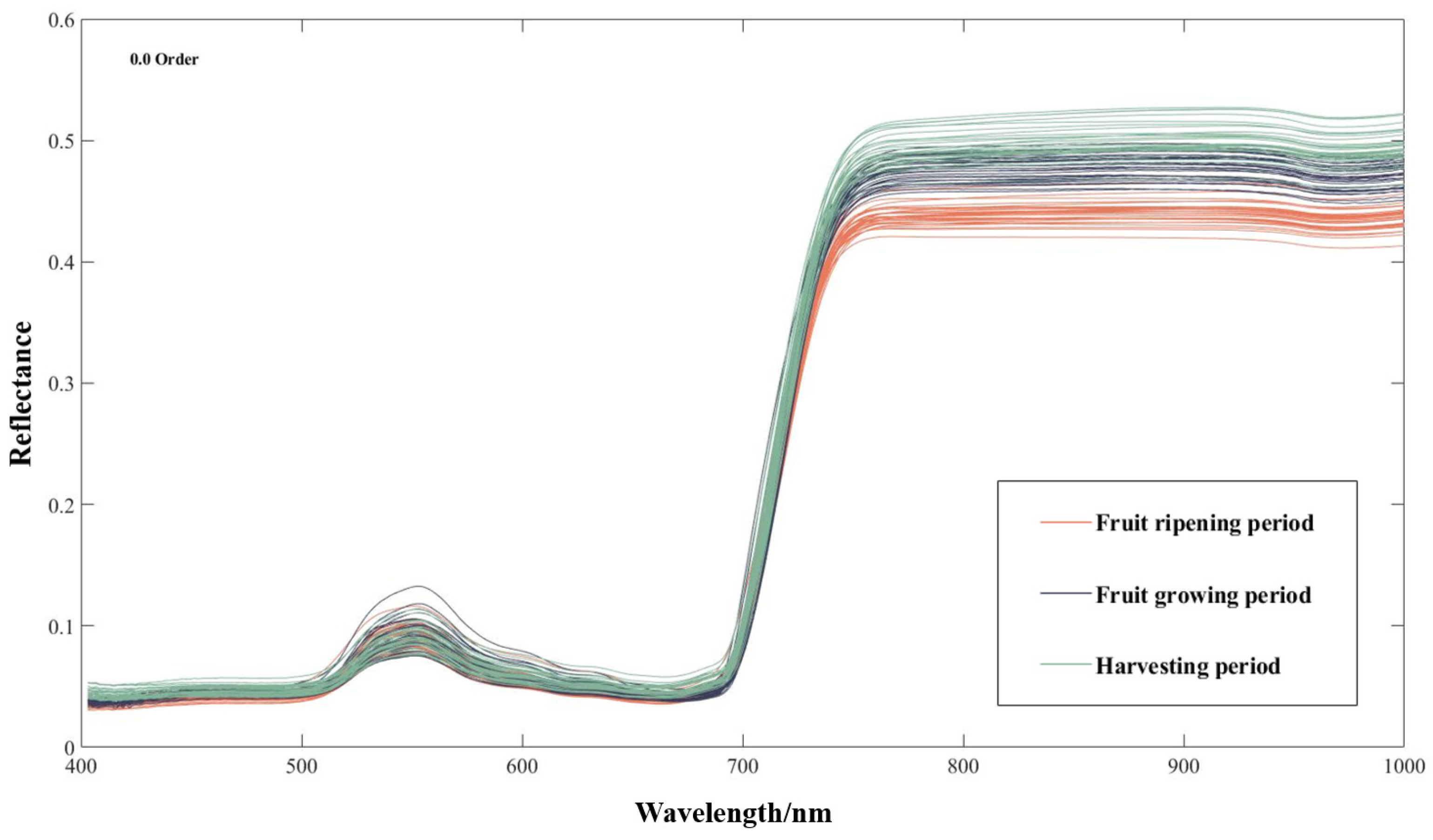
As can be seen in Figure 3, the trends of the reflectance spectral curves of grape leaves at different periods and species are consistent. This is due to the fact that the green plant spectrum is caused by the absorption of light by chlorophyll, other biochemicals and cellular structures on the leaf surface. Therefore, their spectra are basically the same, but due to the different biochemical components, the local details of the curves are quite different [43].
The original spectrum has a distinct peak in the green and visible regions, often called the “green peak”, which is the non-absorbable part of the plant’s photosynthesis process, and therefore has a high spectral reflectance. Near 680 nm in the red-light region, a clear absorption valley is formed due to the strong absorption properties of leaves for red light. After that the absorption of light by the leaf decreases, the reflectance spectral curve rises sharply and forms a high reflectance plateau in the near-infrared band. Grape LCC shows a tendency to increase and then decrease with the period of fertility, causing some changes in LCC due to the differences in the growth cycle between the two sites. During the berry growth period, the leaves undergo sufficient photosynthesis to produce organic matter, and as large amounts of chlorophyll are synthesized, the LCC increases. At maturity, where leaves begin to senesce, chlorophyll starts to decompose and translocate towards being synthesized in newer leaves, resulting in a lower LCC. As chlorophyll levels increased, leaves with lower chlorophyll content had the highest reflectance in the visible range and the lowest reflectance in the near-infrared band. Visible light area leaf spectral reflectance change is most obvious near 550 nm, in the near-infrared band leaf spectral reflectance change is most obvious near 760 nm. It shows that the spectral reflectance of grapes has a strong correlation with LCC. Through the inversion of the change rule of spectral characteristics chlorophyll content, the growth information of grapes can be obtained, so that the real-time state can be based on the reasonable and timely fertilization, to ensure that the grapes have a better growth potential.
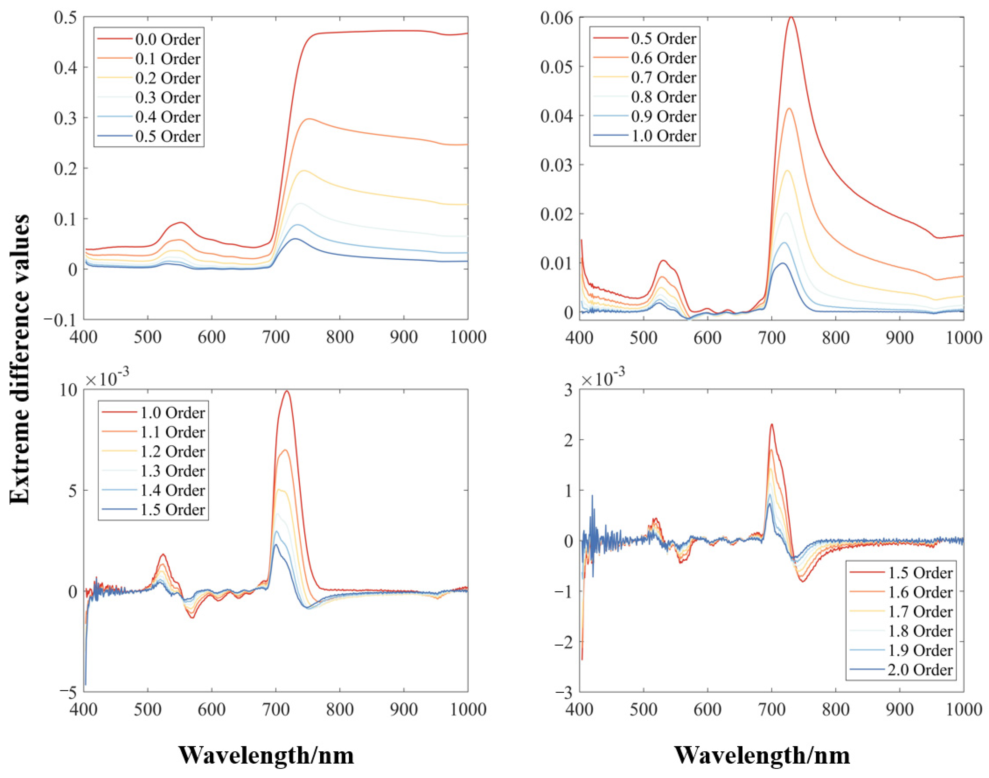
As shown in Figure 4, the raw spectra were subjected to FOD at 0.1-order intervals to obtain 20 fractional-order transformed spectra. There was a significant difference between the results of low-order FOD (0.1–1.0 order) and high-order FOD (1.1–2.0). As the order gradually increases from 0.1 to 1, the differential curves of each order slowly approach the 1st-order differential curves, portraying a variety of changes from 0th- to 1st-order differentiation. When the number of orders gradually increases from 1 to 2, the differential curves of each order slowly approach the 2nd-order differential curves, which describe in detail the fine-tuning difference between the slope and curvature, indicating that FOD has the sensitivity to the slope and curvature of the spectral reflectance curves. Low-order FOD maintains a spectral profile similar to the vegetation spectrum, especially for the water and oxygen absorption valley region (near 760 nm). In contrast, the spectral curves after higher-order FOD treatment showed an obvious loss of morphological features in the vegetation spectral curves as the order increased, with a corresponding increase in the noise peaks and a greater concentration of values, and the orders became indistinguishable throughout the frequency band. Therefore, from the spectral characterization point of view, it is initially judged that low-order FOD can better handle hyperspectral data.
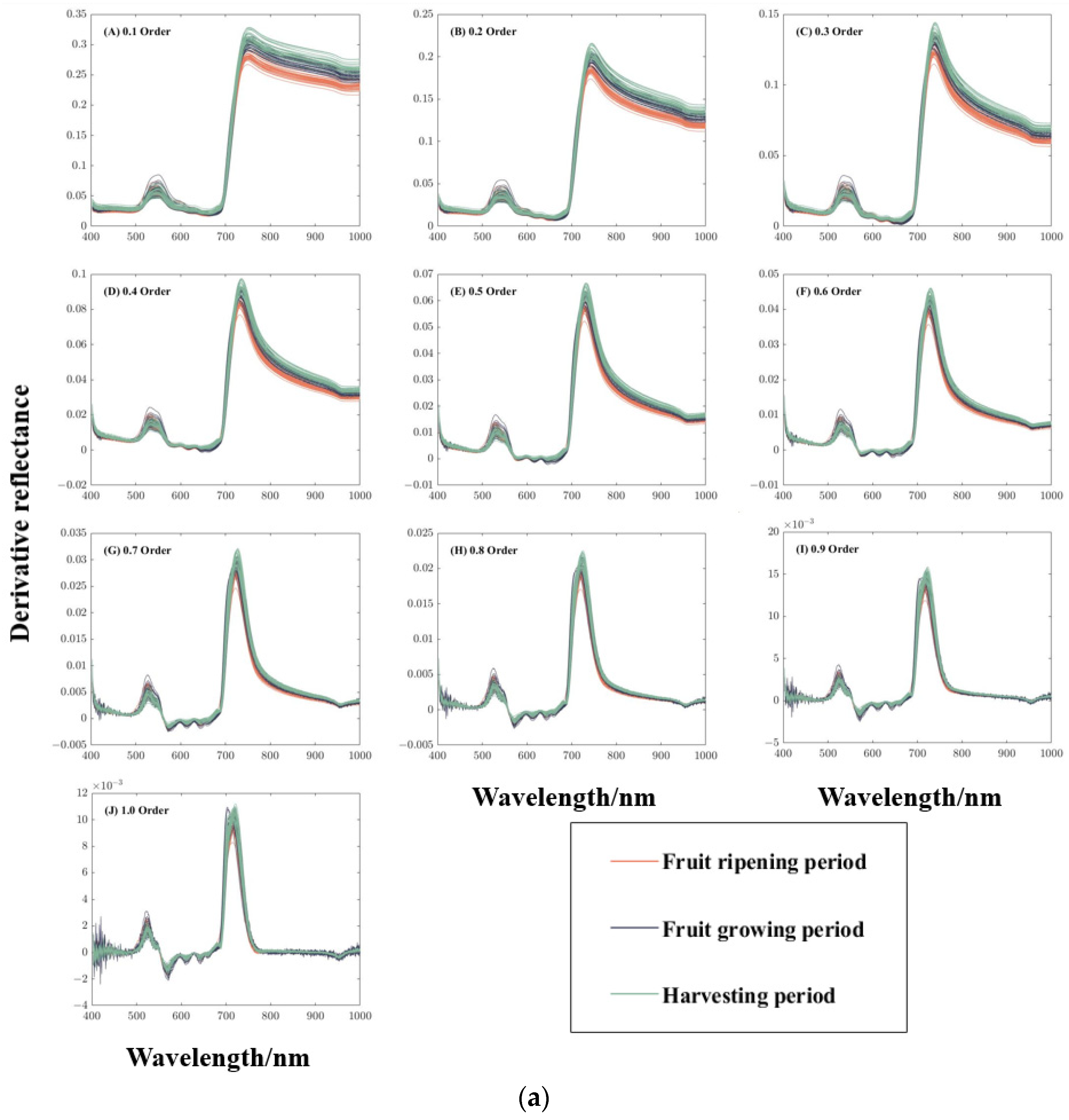
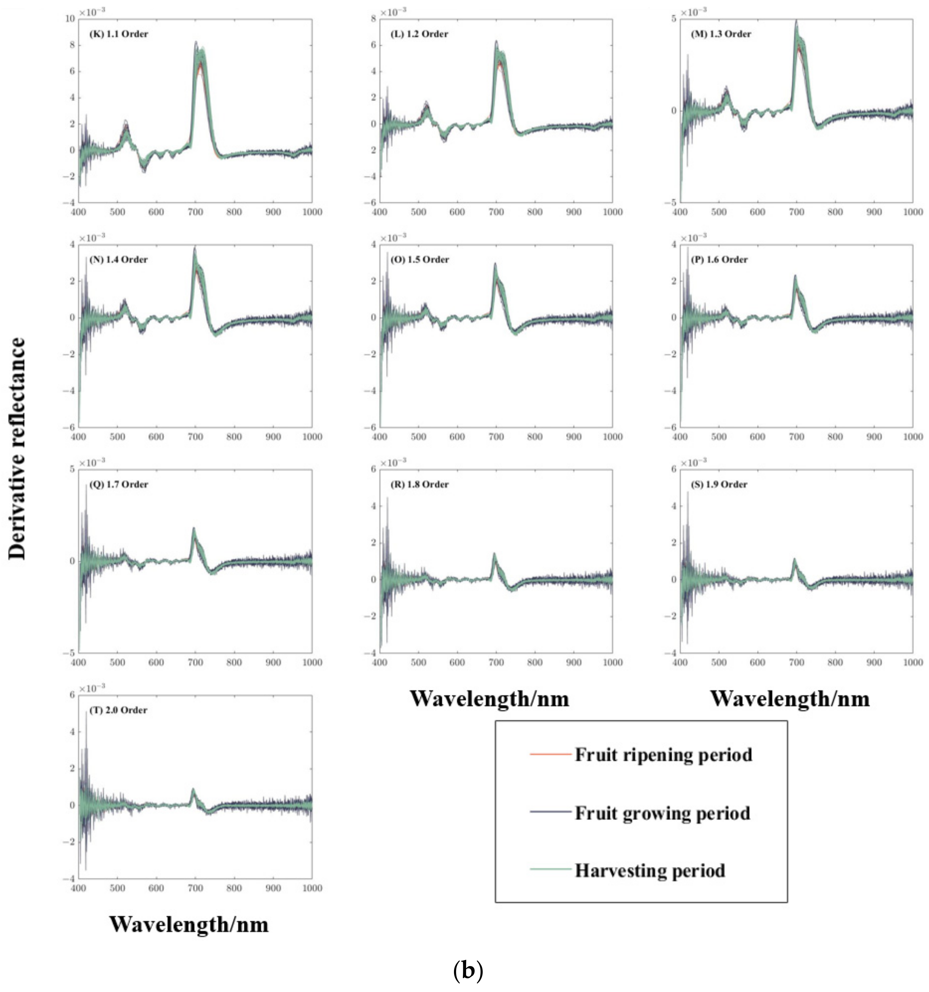
Figure 5 represents the FOD spectral curves for different periods. Figure 5a represents the 0.1–1.0-order differential spectral curve. With the gradual increase in the fractional order, the reflectance differential value gradually decreases and approaches the value of 0. This is because the increment of the order gradually changes the peak profile of the spectral peaks and the de-peaking operation in the differential calculation process. Starting from the 0.4 order, the full-spectrum reflectance is already below 0.1 and is negative in some bands, fluctuating up and down around the 0 value. The entire spectral curve of order 0.1–1.0 is smoother and is in close agreement with the trend of the original spectral curve. The original spectral curve has green peaks, red valleys, and the phenomenon of a near-infrared high reflectance plateau. FOD displays the details of the changes in the reflectance differential values in the process of differential calculations accurately, improves the ability to distinguish between spectral peaks, and makes the peaks and valleys more obvious.
Figure 5b represents the 1.0–2.0-order differential spectral curve. After order 1.0, the trend of the spectral curve gradually slows down. As the order increases, the curve becomes less smooth and more bulges appear, indicating that FOD, while amplifying the subtle differences between the spectral bands, concentrates the distribution. After order 1.2, for higher order FODs, the differences between spectra are amplified in the calculations due to the presence of peaks and valleys of a certain width in the reflectance. The spectral information is enhanced as the order continues to increase and the sampling step is smaller than the width of these peaks and valleys. However, differential arithmetic results in noise with large differences between neighboring bands, which will again amplify the shorter-spaced peaks and valleys, thus introducing high-frequency noise. The noise is more obvious after 1.5 orders, and the spectral curves show a lot of jaggedness, which further indicates that the low-order FOD can achieve effective noise reduction based on amplifying the difference of spectral bands, thus refining the spectra and improving the accuracy of the model.
Integer-order differentiation ignores the gradual change information of the spectrum, which easily causes the signal to go missing while eliminating the noise and affects the prediction accuracy of the chlorophyll content in grape leaves. The differential calculation process is a method to increase the resolution of the spectral signal, and the differential processing of spectral reflectance data enhances the fine variations in the spectral curves on the slope and removes the effect of partially linear and near-linear background and noise on the spectra of grape leaves. As the order increases, the curves begin to become less smooth with smaller bumps, indicating that the fractional order amplifies the microscopic differences between the spectral bands and that the peaks and valleys are becoming more pronounced. The overlap of FOD in different periods becomes higher with the increase in order. This may be because FOD can better concatenate the in-window points and all the previous point bands, so that it is not only dependent on the growth characteristics of the crop to decide. It better reflects the description of FOD on the nonlocal behaviors and long-term dependence of the complex system, which is important for improving the accuracy of the generalized model in different periods.

3.2. Trends in Correlation Coefficients

3.2.1. Effect of FOD on Full-Band Correlation Coefficient

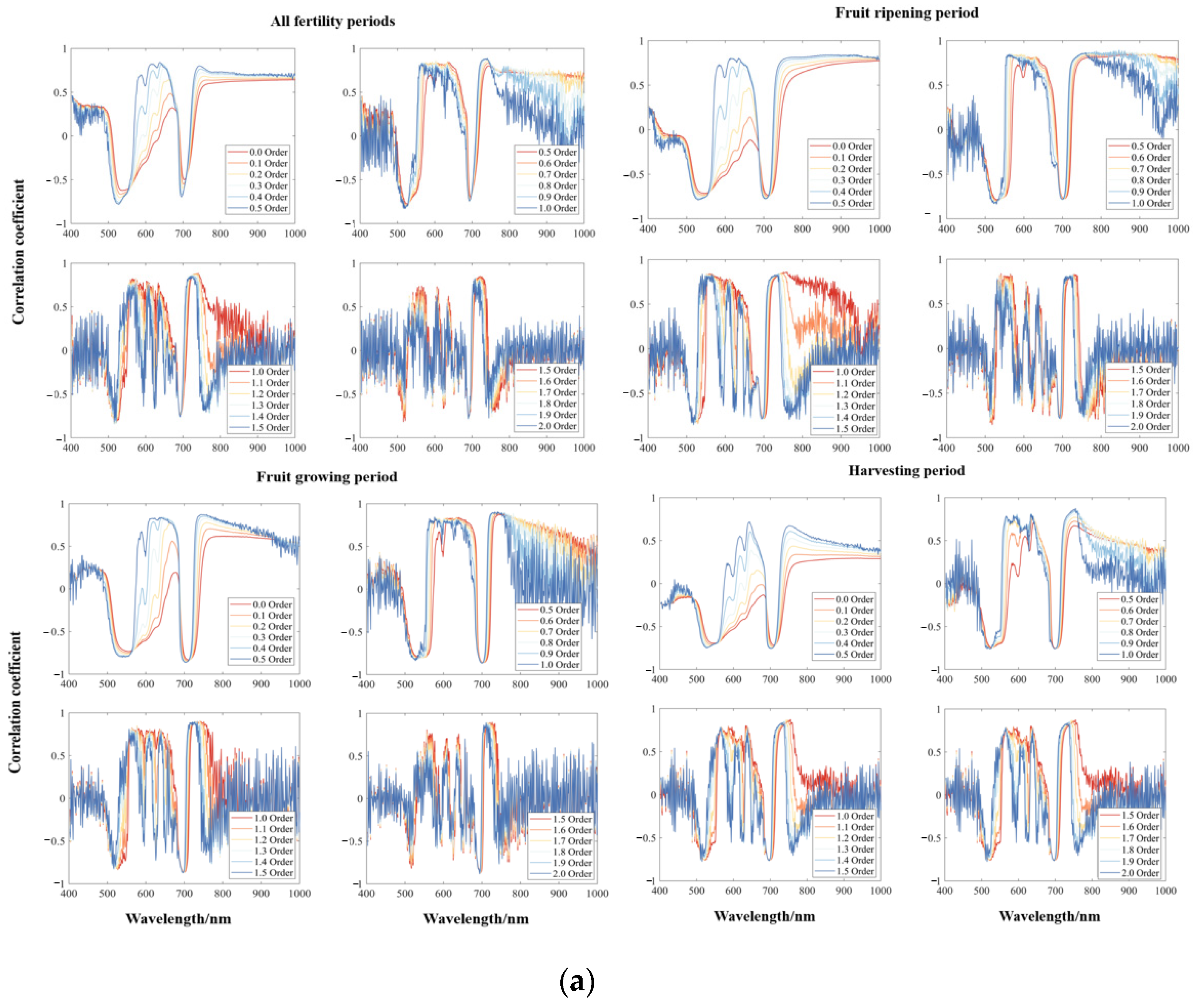
Correlation analysis is widely used to visualize the linear correlation between spectral reflectance and LCC: the higher the correlation the better the linear prediction. Figure 6a shows the correlation between the different-order spectra and the LCC, and it can be seen that the correlations are significantly different. In the lower-order FOD, the correlation coefficient curves are smoother and have a similar trend. Grapevine leaves at different periods were significantly more correlated in the full range of bands than in the original spectra, and there was a trend toward an increase in the number of bands that passed the test for the level of highly significant correlation. The correlation coefficients of higher-order FODs fluctuate frequently between neighboring bands, and the correlation coefficients of orders 1.1~1.5 show large fluctuations and become chaotic between neighboring bands, but it can be seen that the correlation coefficients in the visible region are mostly positive. After order 1.5, the whole curve alternates between positive and negative correlation, strong and weak correlation, with a clear lack of regularity.
The raw spectra were significantly negatively correlated with the chlorophyll content in the green and yellow bands at 510–610 nm and in the red-edge band at 690–740 nm. A significant positive correlation was observed in the near-infrared region of 750–1000 nm. Grape leaf reflectance spectra in the visible range are mainly influenced by leaf pigmentation, with stronger absorption and lower reflectance, and LCC is negatively correlated with the original spectra in this range, suggesting that the higher the LCC, the lower the spectral reflectance and the stronger the absorption. A significant positive correlation was observed in some bands outside the visible range, probably influenced by cell structure and leaf water content. In order 0.1–0.5, the correlation between FOD and SPAD at 580–650 nm increases gradually with the increase in order. Almost all bands in this interval reach significant correlation in order 0.5–1.0, but the correlation in the invisible region of 750 nm begins to decrease and fluctuates frequently with the increase in order, and does not reach significant correlation at 800–1000 nm. At the 1.1–2.0 order, multiple significant positive and negative correlation peaks appeared, but there was little variation in the spectral region through the significant correlation levels. Therefore, bands in this range of 440–800 nm were selected to construct vegetation indices for subsequent analysis and modeling.
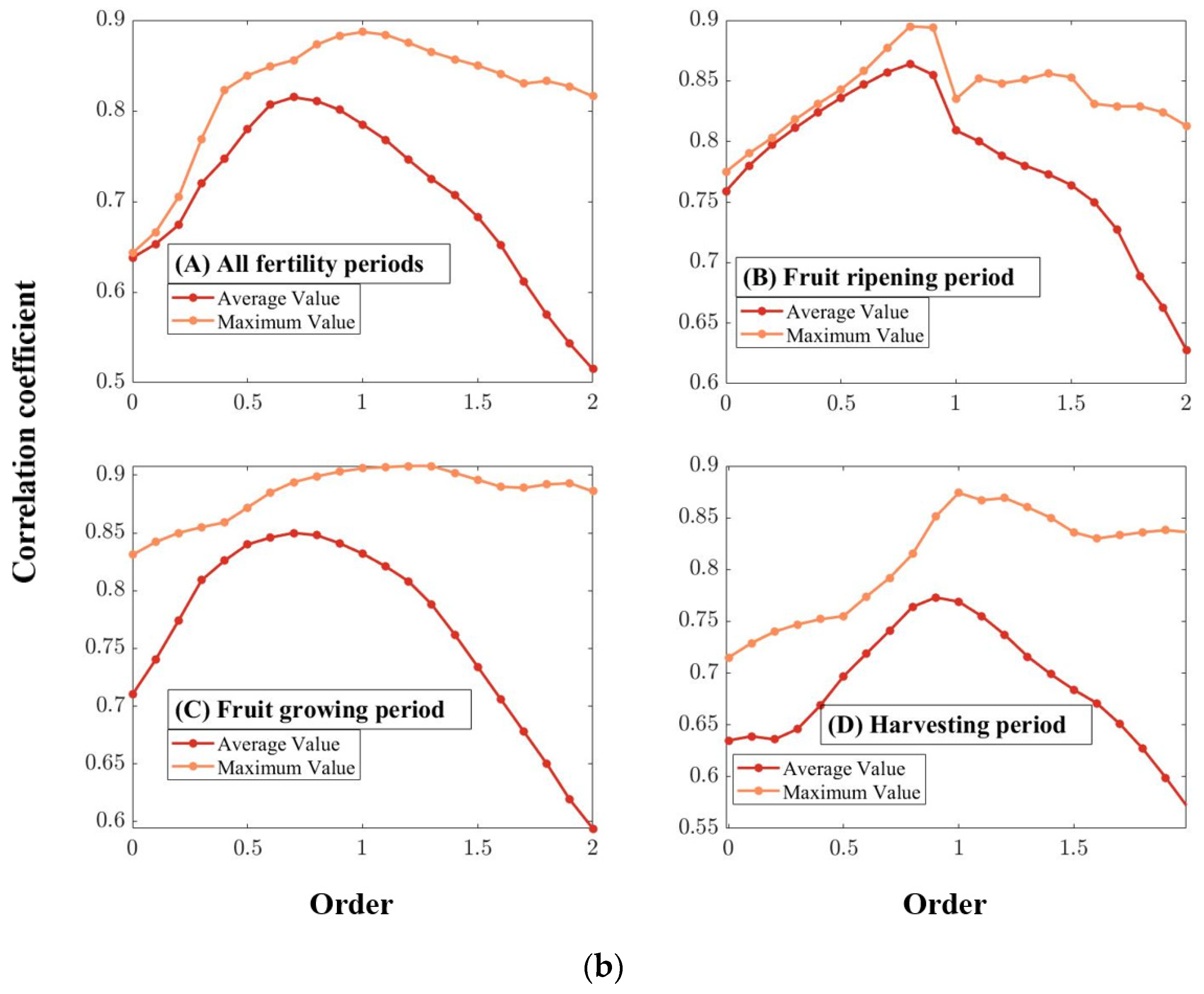
Figure 6b represents the maximum values of the correlation coefficients between FOD and SPAD of each order for different periods, and 20% of the bands with the largest absolute values were selected and averaged. Stable type through the maximum value representing the correlation level and the absolute value representing the correlation level. From the figure, it can be seen that both the maximum value and the mean value showed a trend of increasing and then decreasing as the order increased, and the order with the highest correlation level varied in different fertility periods, which is consistent with the previous conclusion.
Table 2 represents the optimal number of orders for different time periods. In all the reproductive periods, the mean and maximum values occurred at 0.7 and 1.0 orders. Berry’s growth period occurred at 0.8 and 1.2 orders. The maturation period occurred at 0.8 orders. The harvesting period occurred at 0.9 and 1.0 orders. It can be seen that FOD can effectively enhance the correlation level and improve the model accuracy, but the optimal order corresponding to different periods is different.

3.2.2. Effect of FOD on vegetation indices

Spectral indices composed of combinations of correlated bands in linear or nonlinear form capture spectral signals, enhance sensitive information, and reduce interference from correlated noise [44]. Therefore, the vegetation indices used in this study were determined based on the participation of the above-mentioned bands with significant correlation in the calculation. To determine the fractional order and its corresponding bands suitable for the prediction of SPAD in grape leaves, the vegetation indices sensitive to SPAD were constructed, which mainly consisted of 18 vegetation indices as follows (Table 3).
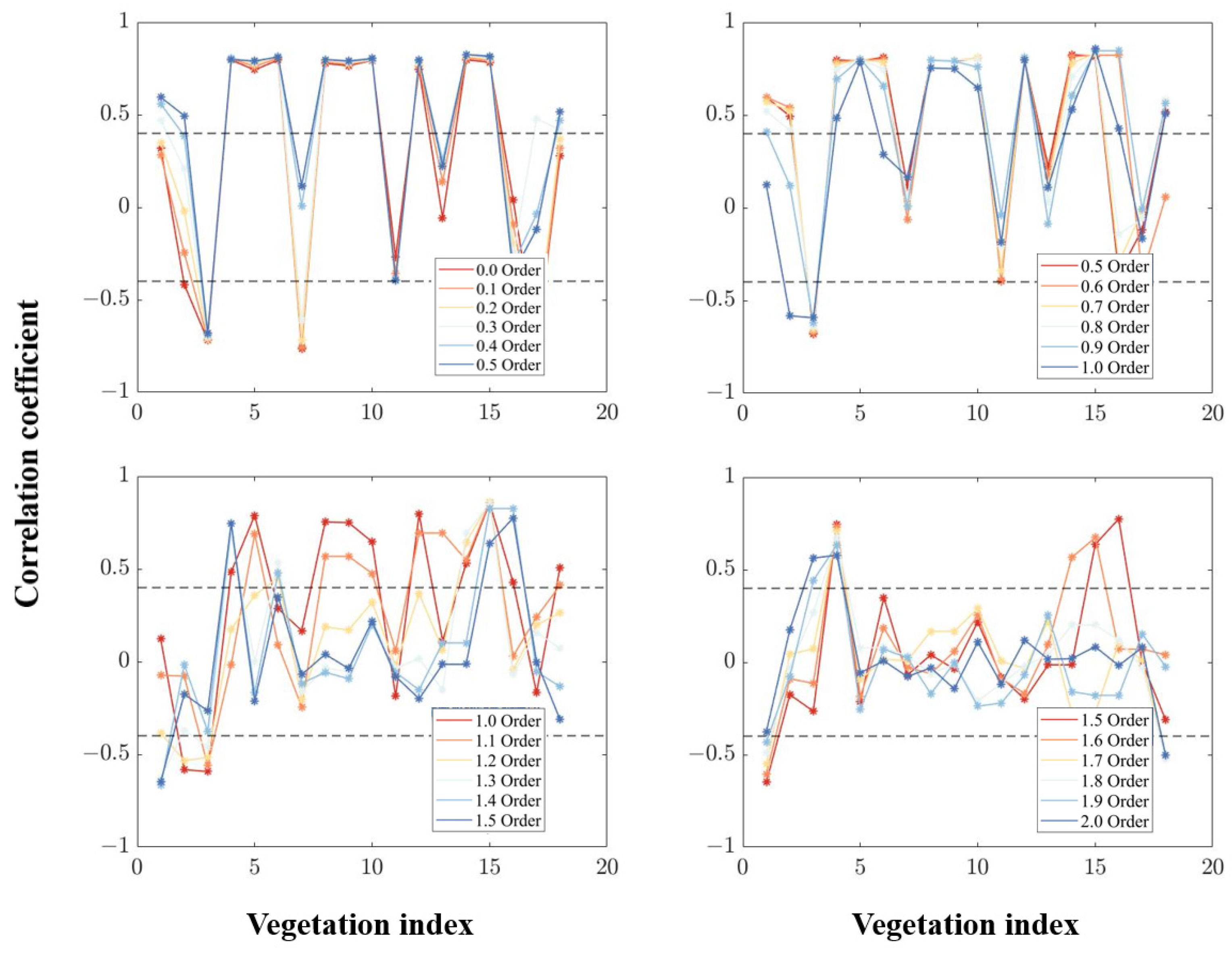
The correlation between the vegetation indices composed of each order of FOD and SPAD is shown in Figure 7. Vegetation indices that reached significant correlation levels varied across orders and tended to decrease with increasing order; after 1.2 orders the number of vegetation indices that reached significant correlation decreased sharply.
The best correlations of raw spectra and FOD with SPAD and its corresponding vegetation indices are shown in Table 4. The optimal correlation coefficient tends to increase and then decrease with increasing order, reaching a maximum at order 1.2 (0.862). The optimal correlation coefficients of orders 0.1–1.4 are all improved over the original spectra, with an improvement of 0.065 in order 1.2, and smaller than the original spectra from order 1.5 onwards. The number of vegetation indices reaching significant correlation at low order FOD stabilized at around 13, but the amount of high-order FOD decreased sharply from order 1.2 onwards, since high-order FOD resulted in fewer bands passing the level of significant correlation and lower correlation coefficients, which in turn constituted vegetation indices that were lowly and sparsely correlated with SPAD.

3.3. SPAD Prediction Model for Grapes Based on FOD-RFR

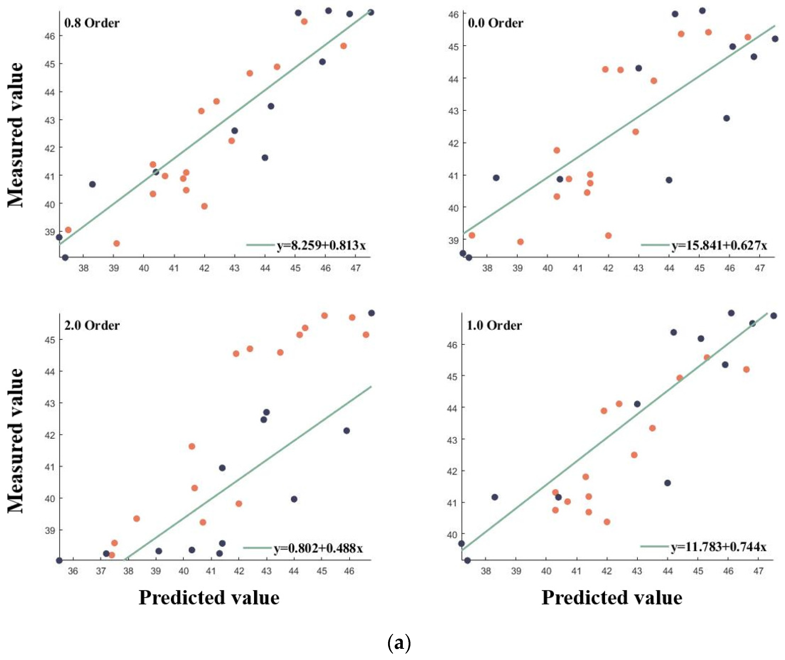
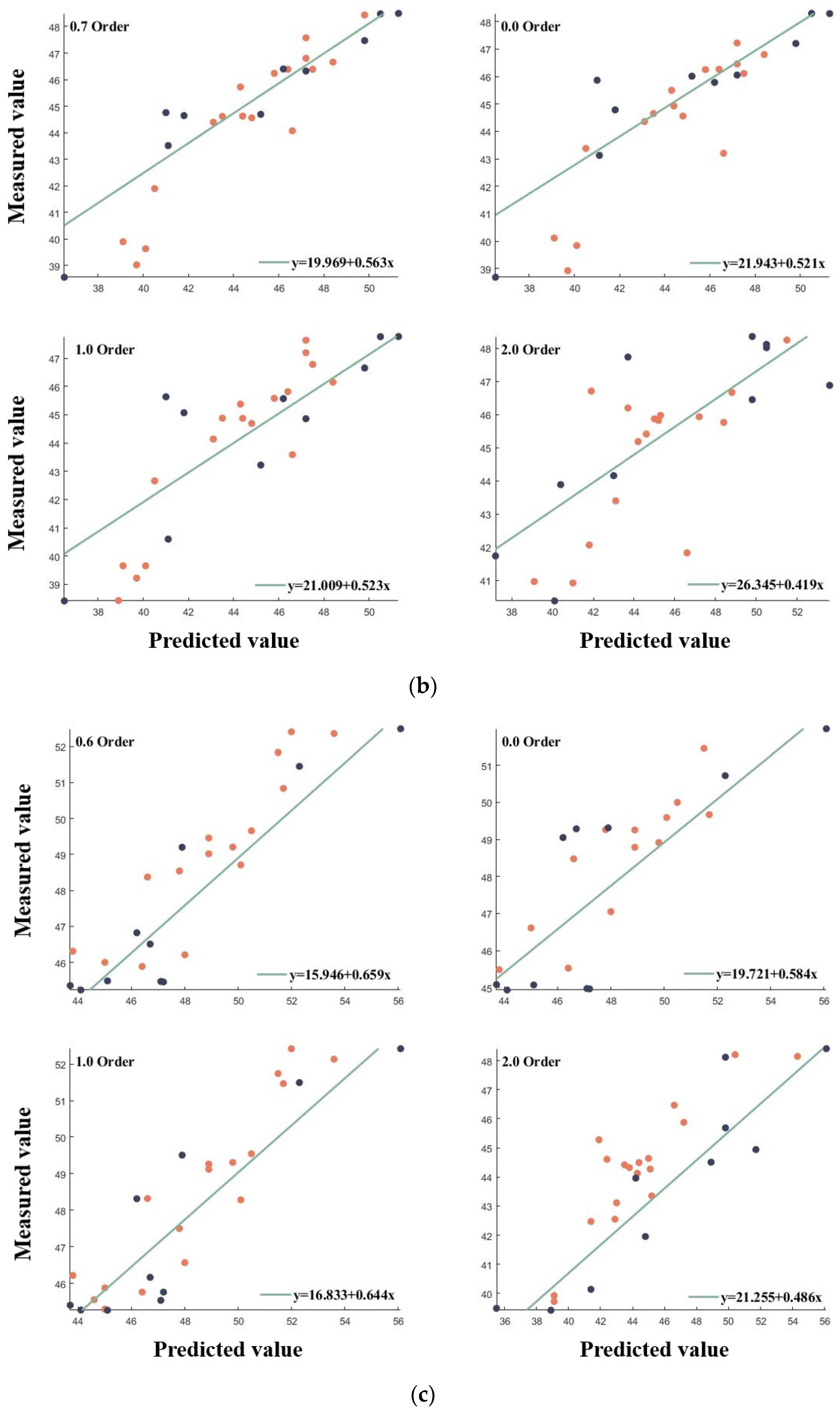
To further confirm the ability of FOD to predict LCC in grapes, this study used FOD spectra that included raw spectra and FOD spectra of 0.1–2.0 orders (with 0.1 order intervals) during the growing, ripening, and harvesting stages of the berry to comparatively analyze them. Based on the significance test of the correlation coefficient to screen the sensitive bands, we constructed the typical vegetation indices corresponding to different orders as the model input parameters, and finally used the RFR method to establish the LCC prediction model for grapes in different periods. By evaluating the uniformity of the three periods, we analyzed whether there was any universality to the FOD that could enhance the effect of the model in different fertility periods. The ratio of training sets to test sets in the study was 7:3, and they are represented in Figure 8 and Figure 9 by orange and black colors. FOD and RFR were both implemented in python. The number of decision trees in the RF model was 1000 and the minimum number of leaves was 5.

3.3.1. Model for Predicting LCC in Grapes at Different Fertility Stages

Table 5a gives the R 2 , RMSE, and NRMSE of the FOD-RFR chlorophyll prediction model for wine grape Cabernet Sauvignon at maturity. From an integer-order perspective, in the LCC prediction model constructed with typical vegetation indices corresponding to the original reflectance spectra, 1st- and 2nd-order differential spectra, the 1st-order model showed an increase of 0.094 in R 2 , and a decrease of 1.186 and 0.8% in RMSE and NRMSE compared to the original spectra. Compared to the 2nd-order spectra, R 2 improved by 0.301, and RMSE and NRMSE decreased by 0.618 and 1.6%, indicating that the first-order differentiation favored the prediction of LCC at the mature stage. After refining the differentiation interval to the order of 0.1, the R 2 of the model showed an overall trend of increasing and then decreasing, the RMSE and NRMSE decreased and then increased. The model achieved optimal results at order 0.8, where R 2 = 0.883, RMSE = 1.224, and NRMSE = 2.8%, which was an improvement of 0.094, 0.417, and 1% over the 1st-order spectrum. From order 1.2, the model stability decrease compared to the original spectra, but all of them were better than the 2nd-order differential spectra.
The LCC prediction model for ripening grapes with the highest accuracy 0.8-order differential spectra, raw spectra, and integer-order spectral model scatter plots are shown in Figure 8a. The maximum and mean values of the correlation between leaf spectra and LCC of ripening grapes were of the order of 0.8. By constructing a typical vegetation index through the sensitive bands as model inputs, the model achieved the best prediction at 0.8, indicating that an increase in the sensitivity of the inputs leads to better model accuracy and stability.
Table 5b gives the R 2 , RMSE, and NRMSE of the FOD-RFR chlorophyll prediction model for table grape Sunshine Rose during the berry growth period. In integer-order spectra, the original spectral modes show a 0.055 increase in R 2 and a 0.218 and 0.5% decrease in RMSE and NRMSE compared to the 1st-order spectra. Compared to the 2nd-order spectra, R 2 increased by 0.123 and RMSE and NRMSE decreased by 0.94 and 1.9%, indicating that the raw spectra were favorable for the prediction of LCC during the berry growth period. In FOD, multiple peaks appear as the order rises, which are located at the 0.7, 1.3, and 1.8 orders, with the best prediction at the 0.7 order, where R 2 = 0.761, RMSE = 2.254, and NRMSE = 5%, which are up and down by 0.062, 0.284, and 6%, compared to the original spectra.
The berry growing season grape LCC prediction model with the highest accuracy 0.7 order differential spectra, raw spectra, and integer-order spectral model scatter plots are shown in Figure 8b. The maximum and mean values of the correlation between leaf spectra and LCC of ripening grapes were 0.8 and 1.2 orders, but the model achieved the best prediction at 0.7 order, suggesting that the accuracy of the model depends not only on the parameter with the best correlation, but also on the overall correlation of the parameters.
Table 5c gives the R 2 , RMSE, and NRMSE of the FOD-RFR chlorophyll prediction model for table grape Sunshine Rose at harvest. In integer-order spectra, the 1st-order spectral model improves R 2 by 0.138 and decreases RMSE and NRMSE by 0.458 and 0.9% compared to the original spectra. Compared with the 2nd- order spectra, R 2 increased by 0.243, and RMSE and NRMSE decreased by 2.378 and 5.2%, indicating that the first-order differentiation was favorable for the prediction of LCC during the growing period of berries. After refining the differentiation interval to the order of 0.1, the R 2 of the model shows an overall trend of increasing and then decreasing, the RMSE and NRMSE are decreasing and then increasing. The model achieved optimal results at order 0.6, where R 2 = 0.807, RMSE = 1.593, and NRMSE = 3.3%, which is an improvement of 0.038, 0.149, and 0.4% over the order 1 spectrum.
The grape LCC prediction model for the harvest period has the highest accuracy of 0.6 order differential spectra, raw spectra, and integer-order spectral model scatter plots are shown in Figure 8c. The maximum and mean values of the correlation between grape leaf spectra and SPAD at harvest were 0.9 and 1.0 orders, respectively. Typical vegetation indices were constructed as model inputs through sensitive bands, and the model achieved the best prediction at 0.6 order.

3.3.2. Grape LCC Prediction Model for the Full Life Span

The accuracy of the FOD-treated prediction model was improved over the integer-order model at all fertility periods, and to determine whether this conclusion held for different varieties of grapes over the full fertility period, selected samples from the three fertility periods were subjected to disordered order treatment and then verified uniformly.
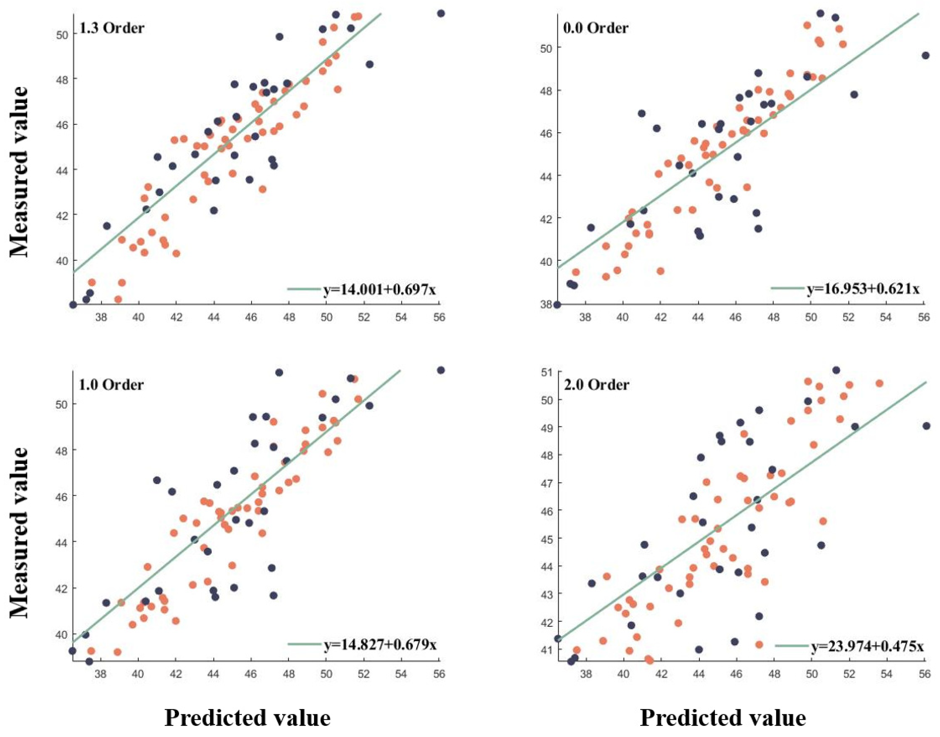
Table 6 represents the R 2 , RMSE, and NRMSE of the FOD-RFR chlorophyll prediction model over the full life span. From an integer-order perspective, in the LCC prediction model constructed with typical vegetation indices corresponding to the original reflectance spectra, 1st- and 2nd-order differential spectra, the 1st-order model showed an increase of 0.025 in R 2 and a decrease of 0.09 and 0.2% in RMSE and NRMSE compared to the original spectra. Compared to the 2nd-order spectra, R 2 improved by 0.169 and RMSE and NRMSE decreased by 0.919 and 1.3% indicating that the first-order discretization was favorable for the prediction of LCC over the whole reproductive period. After refining the differentiation interval to order 0.1, two peaks in the R 2 of the model appear, which are located in order 0.5 and 1.3, both of which have higher accuracy than the integer-order model. In order 0.5, the model improved R 2 , RMSE, and NRMSE by 0.092, 0.361, and 0.8% compared to the order 1 model. In order 1.3, the model improved R 2 , RMSE, and NRMSE by 0.148,0.609, and 1.3% compared to the order 1 model.
Scatter plots of 1.3-order differential spectra, raw spectra, and integer-order spectral modeling scatter plots for the full-birth grape LCC prediction model with the highest accuracy are shown in Figure 9. The maximum and mean values of the correlation between grape leaf spectra and SPAD at harvest were 0.7 and 1.0 orders, respectively. Typical vegetation indices were constructed as model inputs through sensitive bands, and the model achieved the best prediction at 1.3 orders. This occurs because the correlation of features varies in different fertility periods, and when selecting the best-dividing features, only a fraction of the randomly selected features are considered, placing certain features that have a disproportionate effect on the whole model, and thus improving the robustness of the model.

4. Discussion

Leaf chlorophyll content is an important indicator of plant growth and development, and many researchers have conducted studies related to the remote sensing estimation of leaf chlorophyll content [59,60]. Most of the studies use integer-order differentiation, a common preprocessing method for hyperspectral data, which has some potential for application. However, the baseline and noise disturbances, when nonlinear non-stationary signal, will not increase or decrease proportionally, meaning the integer order cannot solve this kind of problem well, thus affecting the model accuracy [61]. FOD, as an extension of integer order, can deeply explore the asymptotic information of spectra while promoting the significance of integer order. A large number of studies have shown that FOD can effectively improve the correlation coefficients between spectral bands and target variables [62,63]. Therefore, the present study attempted to explore its ability to estimate the chlorophyll content of grape leaves using fractional-order differential spectroscopy and to analyze the spectra systematically.
In the study, it was found that FOD revealed more information related to LCC by differentiating the spectral reflectance of grape leaves from 0 to 2 orders using 0.1 order as the step size. For example, the low-order FOD in Figure 5a shows the detailed changes in the reflectance differential values during the differential calculation process accurately, which improves the discrimination between spectral peaks and makes the peaks and valleys more obvious. As shown in Figure 5b, the sampling steps in higher-order FOD are smaller than the widths of the peaks and valleys, and the differences between the spectra are amplified in the calculations, thus enhancing the spectral information. After correlation analysis with LCC, it can be seen that FOD enhances the correlation between bands and target variables; the number of sensitive bands is also enhanced, and many studies have confirmed this phenomenon [64,65].
Vegetation index combines different feature sensitivities continuously by difference and ratio algorithms, which can better capture the spectral signals, enhance the sensitivity information, and reduce the interference of correlated noise [66]. Mathematical modeling using vegetation indices is a common method used in chlorophyll content inversion studies [67]. The study constructed 18 vegetation indices with strong correlation with LCC adopted by most studies. When analyzing the correlation between each order of vegetation indices and LCC, the low-order FOD enhanced the best coefficients of each order, and the number of indices passing the level of significance did not differ much from the original spectra. The optimal coefficients reach the maximum at order 1.2, but the number of indices decreases significantly and gradually approaches 0 as the order increases, which is since higher-order FOD introduces certain high-frequency noise while improving accuracy. Therefore, in using FOD for spectral preprocessing, the effect produced by different orders varies significantly, and choosing the appropriate order for processing is the key to building a prediction model.
In the modeling process, the study used a typical machine learning algorithm, the random forest regression algorithm. Due to the nature of random forest, it can better highlight the effect of fractional-order spectra on the modeling results. The final regression prediction results are obtained by averaging the prediction results of each decision tree [68]. Machine learning and deep learning are increasingly used to analyze crop growth metrics, and the applicability of processing hyperspectral data through FOD to the remaining models can be explored in future research.
In this study, based on the growth stages of different varieties of grapes at three fertility periods. The orders corresponding to the optimal models at different stages varied, but all of them were improved compared with the integer-order models, and the same conclusions were obtained on the whole fertility period, which indicated that preprocessing the spectra by fractional order was feasible for improving the model accuracy. The applicability of this conclusion to other varieties and varieties with large differences in growth periods is debatable due to the conditions, so the generalizability of the technique for the prediction of chlorophyll content in grape leaves could be improved by increasing the number of experiments in future studies.

5. Conclusions

In this study, the differential spectral characteristics of grapes at different fertility stages were analyzed by the FOD process of hyperspectral data, and typical vegetation indices were constructed based on the sensitive bands related to LCC to establish a high-precision model for the prediction of LCC in grapes, the following conclusions were drawn:
(1)
There was better sensitivity between the FOD spectra and grape LCC compared to the raw spectra, with the best correlation improving from 0.797 (order 0) to 0.862 (order 1.2) and the best coefficients of most of the differential spectra improved compared to the raw spectra.
(2)
The FOD-RFR chlorophyll prediction models for different fertility stages all had improved accuracy over the integer order, but the optimal order of the models differed for different fertility stages, with 0.8 order for ripening, 0.7 order for berry growth, and 0.6 order for picking. Model accuracy was also improved by applying the model to the full maturity period, with an optimal order of 1.3, where R 2 = 0.778, RMSE = 2.1, and NRMSE = 4.7%. This suggests that fractional-order discretization methods can be applied to grape leaf spectral preprocessing, providing theoretical support for improving accurate measurements of grape LCC.
The conclusions of this study apply to the two selected samples of grapes of widely differing varieties and growing periods, but it is not clear whether data collection of the same varieties in different years would lead to the same optimal order of the models found in this study. Therefore, further investigation should be considered in future studies.

Author Contributions

Conceptualization, X.X. and W.W.; writing—original draft preparation, X.Y., Y.Z. and G.Y.; writing—review and editing, Y.L., Y.M., X.J. and H.X. All authors have read and agreed to the published version of the manuscript.

Funding

This study was supported by Key Science and Technology Special Project of Yunnan Province (No. 202202AE090013-2), National Natural Science Foundation (No. 42371323), National Key Research and Development Program (No. 2023YFD2300503) and National Modern Agricultural Industry Technology System (No. CARS-03).

Data Availability Statement

The data that support the findings of this study are available from the corresponding author, upon reasonable request.

Conflicts of Interest

The authors declare no conflicts of interest.

References

  1. Yang, Z.; Tian, J.; Feng, K.; Gong, X.; Liu, J. Application of a hyperspectral imaging system to quantify leaf-scale chlorophyll, nitrogen and chlorophyll fluorescence parameters in grapevine. Plant Physiol. Biochem. 2021, 166, 723–737. [Google Scholar] [CrossRef]
  2. Wu, C.; Niu, Z.; Tang, Q.; Huang, W. Estimating chlorophyll content from hyperspectral vegetation indices: Modeling and validation. Agric. For. Meteorol. 2008, 148, 1230–1241. [Google Scholar] [CrossRef]
  3. Zhang, P.; Dong, T.; Jin, H.; Pei, D.; Pervaiz, T.; Ren, Y.; Jia, H.; Fang, J. Analysis of photosynthetic ability and related physiological traits in nodal leaves of grape. Sci. Hortic. 2022, 304, 111251. [Google Scholar] [CrossRef]
  4. Rey-Caramés, C.; Aguila, J.T.; Sanz-Garcia, A.; Chica-Olmo, M.; Diago, M.P. Quantifying spatio-temporal variation of leaf chlorophyll and nitrogen contents in vineyards. Biosyst. Eng. 2016, 150, 201–213. [Google Scholar] [CrossRef]
  5. Yang, X.; Yang, R.; Ye, Y.; Yuan, Z.; Wang, D.; Hua, K. Winter wheat SPAD estimation from UAV hyperspectral data using cluster-regression methods. Int. J. Appl. Earth Obs. Geoinf. 2021, 105, 102618. [Google Scholar] [CrossRef]
  6. Wojdyło, A.; Nowicka, P.; Tkacz, K.; Turkiewicz, I.P. Fruit tree leaves as unconventional and valuable source of chlorophyll and carotenoid compounds determined by liquid chromatography-photodiode-quadrupole/time of flight-electrospray ionization-mass spectrometry (LC-PDA-qTof-ESI-MS). Food Chem. 2021, 349, 129156. [Google Scholar] [CrossRef]
  7. Ahmad, N.A.; Muttalib, M.F.A.; Uda, M.N.A.; Arsat, Z.A.; Abdullah, F.; Hashim, M.K.R.; Azizan, F.A.; Jusoh, M.F.; Kamaruzaman, S.R.S.; Nordin, A.A. Measurement of leaf chlorophyll content in Harumanis mango cultivated in a greenhouse using SPAD meter. Mater. Today Proc. 2023; in press. [Google Scholar] [CrossRef]
  8. Liu, N.; Hokanson, E.W.; Hansen, N.; Townsend, P.A. Multi-year hyperspectral remote sensing of a comprehensive set of crop foliar nutrients in cranberries. ISPRS J. Photogramm. Remote Sens. 2023, 205, 135–146. [Google Scholar] [CrossRef]
  9. Song, D.; De Silva, K.; Brooks, M.D.; Kamruzzaman, M. Biomass prediction based on hyperspectral images of the Arabidopsis canopy. Comput. Electron. Agric. 2023, 210, 107939. [Google Scholar] [CrossRef]
  10. Flynn, K.C.; Baath, G.; Lee, T.O.; Gowda, P.; Northup, B. Hyperspectral reflectance and machine learning to monitor legume biomass and nitrogen accumulation. Comput. Electron. Agric. 2023, 211, 107991. [Google Scholar] [CrossRef]
  11. Lv, S.; Wang, J.; Wang, Z.; Fang, Y.; Wang, S.; Wang, F.; Wang, X.; Qu, G.; Ma, W. Construction of hyperspectral reflectance and spectral index inversion model for the water content of Catalpa bungei leaves. Microchem. J. 2024, 197, 109811. [Google Scholar] [CrossRef]
  12. Guo, A.; Ye, H.; Huang, W.; Qian, B.; Wang, J.; Lan, Y.; Wang, S. Inversion of maize leaf area index from UAV hyperspectral and multispectral imagery. Comput. Electron. Agric. 2023, 212, 108020. [Google Scholar] [CrossRef]
  13. Rajewicz, P.A.; Zhang, C.; Atherton, J.; Van Wittenberghe, S.; Riikonen, A.; Magney, T.; Fernandez-Marin, B. Jose Ignacio Garcia Plazaola, Albert Porcar-Castell, The photosynthetic response of spectral chlorophyll fluorescence differs across species and light environments in a boreal forest ecosystem. Agric. For. Meteorol. 2023, 334, 109434. [Google Scholar] [CrossRef]
  14. Huang, X.; Guan, H.; Bo, L.; Xu, Z.; Mao, X. Hyperspectral proximal sensing of leaf chlorophyll content of spring maize based on a hybrid of physically based modelling and ensemble stacking. Comput. Electron. Agric. 2023, 208, 107745. [Google Scholar] [CrossRef]
  15. Li, X.; Wei, Z.; Peng, F.; Liu, J.; Han, G. Estimating the distribution of chlorophyll content in CYVCV infected lemon leaf using hyperspectral imaging. Comput. Electron. Agric. 2022, 198, 107036. [Google Scholar] [CrossRef]
  16. Zhao, R.; An, L.; Tang, W.; Qiao, L.; Wang, N.; Li, M.; Sun, H.; Liu, G. Improving chlorophyll content detection to suit maize dynamic growth effects by deep features of hyperspectral data. Field Crops Res. 2023, 297, 108929. [Google Scholar] [CrossRef]
  17. Li, L.; Ren, T.; Ma, Y.; Wei, Q.; Wang, S.; Li, X.; Cong, R.; Liu, S.; Lu, J. Evaluating chlorophyll density in winter oilseed rape (Brassica napus L.) using canopy hyperspectral red-edge parameters. Comput. Electron. Agric. 2016, 126, 21–31. [Google Scholar] [CrossRef]
  18. Zarco-Tejada, P.J.; Miller, J.R.; Morales, A.; Berjón, A.; Agüera, J. Hyperspectral indices and model simulation for chlorophyll estimation in open-canopy tree crops. Remote Sens. Environ. 2004, 90, 463–476. [Google Scholar] [CrossRef]
  19. Zhang, D.; Zhang, J.; Peng, B.; Wu, T.; Jiao, Z.; Lu, Y.; Li, G.; Fan, X.; Shen, S.; Gu, A.; et al. Hyperspectral model based on genetic algorithm and SA-1DCNN for predicting Chinese cabbage chlorophyll content. Sci. Hortic. 2023, 321, 112334. [Google Scholar] [CrossRef]
  20. Xiao, B.; Li, S.; Dou, S.; He, H.; Fu, B.; Zhang, T.; Sun, W.; Yang, Y.; Xiong, Y.; Shi, J.; et al. Comparison of leaf chlorophyll content retrieval performance of citrus using FOD and CWT methods with field-based full-spectrum hyperspectral reflectance data. Comput. Electron. Agric. 2024, 217, 108559. [Google Scholar] [CrossRef]
  21. Sierociuk, D.; Skovranek, T.; Macias, M.; Podlubny, I.; Petras, I.; Dzielinski, A.; Ziubinski, P. Diffusion process modeling by using fractional-order models. Appl. Math. Comput. 2015, 257, 2–11. [Google Scholar] [CrossRef]
  22. Xu, L.; Shi, S.; Gong, W.; Shi, Z.; Qu, F.; Tang, X.; Chen, B.; Sun, J. Improving leaf chlorophyll content estimation through constrained PROSAIL model from airborne hyperspectral and LiDAR data. Int. J. Appl. Earth Obs. Geoinf. 2022, 115, 103128. [Google Scholar] [CrossRef]
  23. Kusnierek, K.; Korsaeth, A. Simultaneous identification of spring wheat nitrogen and water status using visible and near infrared spectra and Powered Partial Least Squares Regression. Comput. Electron. Agric. 2015, 117, 200–213. [Google Scholar] [CrossRef]
  24. Zhang, Y.; Hui, J.; Qin, Q.; Sun, Y.; Zhang, T.; Sun, H.; Li, M. Transfer-learning-based approach for leaf chlorophyll content estimation of winter wheat from hyperspectral data. Remote Sens. Environ. 2021, 267, 112724. [Google Scholar] [CrossRef]
  25. Lazopoulos, K.A.; Karaoulanis, D.; Lazopoulos, A.K. On fractional modelling of viscoelastic mechanical systems. Mech. Res. Commun. 2016, 78 Pt A, 1–5. [Google Scholar] [CrossRef]
  26. Zhang, J.; Jing, X.; Song, X.; Zhang, T.; Duan, W.; Su, J. Hyperspectral estimation of wheat stripe rust using fractional order differential equations and Gaussian process methods. Comput. Electron. Agric. 2023, 206, 107671. [Google Scholar] [CrossRef]
  27. Area, I.; Losada, J.; Nieto, J.J. A note on the fractional logistic equation. Phys. A Stat. Mech. Appl. 2016, 444, 182–187. [Google Scholar] [CrossRef]
  28. Jin, J.; Wang, Q. Hyperspectral indices developed from the low order fractional derivative spectra can capture leaf dry matter content across a variety of species better. Agric. For. Meteorol. 2022, 322, 109007. [Google Scholar] [CrossRef]
  29. Song, G.; Wang, Q.; Jin, J. Estimation of leaf photosynthetic capacity parameters using spectral indices developed from fractional-order derivatives. Comput. Electron. Agric. 2023, 212, 108068. [Google Scholar] [CrossRef]
  30. Ren, K.; Dong, Y.; Huang, W.; Guo, A.; Jing, X. Monitoring of winter wheat stripe rust by collaborating canopy SIF with wavelet energy coefficients. Comput. Electron. Agric. 2023, 215, 108366. [Google Scholar] [CrossRef]
  31. Abulaiti, Y.; Sawut, M.; Maimaitiaili, B.; Chunyue, M. A possible fractional order derivative and optimized spectral indices for assessing total nitrogen content in cotton. Comput. Electron. Agric. 2020, 171, 105275. [Google Scholar] [CrossRef]
  32. Zhang, J.; Tian, H.; Wang, D.; Li, H.; Mouazen, A.M. A novel spectral index for estimation of relative chlorophyll content of sugar beet. Comput. Electron. Agric. 2021, 184, 106088. [Google Scholar] [CrossRef]
  33. Khan, M.; Kumar, P. A level set based fractional order variational model for motion estimation in application-oriented spectrum. Expert Syst. Appl. 2023, 219, 119628. [Google Scholar] [CrossRef]
  34. Fu, C.; Gan, S.; Xiong, H.; Tian, A. A new method to estimate soil organic matter using the combination model based on short memory fractional order derivative and machine learning model. Infrared Phys. Technol. 2023, 134, 104922. [Google Scholar] [CrossRef]
  35. Gamini, S.; Kumar, S.S. Homomorphic filtering for the image enhancement based on fractional-order derivative and genetic algorithm. Comput. Electr. Eng. 2023, 106, 108566. [Google Scholar] [CrossRef]
  36. Li, C.; Chen, A.; Ye, J. Numerical approaches to fractional calculus and fractional ordinary differential equation. J. Comput. Phys. 2011, 230, 3352–3368. [Google Scholar] [CrossRef]
  37. Kavuran, G. When machine learning meets fractional-order chaotic signals: Detecting dynamical variations. Chaos, Solitons & Fractals 2022, 157, 111908. [Google Scholar] [CrossRef]
  38. Zhao, C.; Shi, L.; Guan, Y.; Li, X.; Shi, Z. Formal modeling and verification of fractional order linear systems. ISA Trans. 2016, 62, 87–93. [Google Scholar] [CrossRef] [PubMed]
  39. Cai, W.-L.; Fang, C.; Liu, L.-F.; Sun, F.-Y.; Xin, G.-Z.; Zheng, J.-Y. Pseudotargeted metabolomics-based random forest model for tracking plant species from herbal products. Phytomedicine 2023, 118, 154927. [Google Scholar] [CrossRef] [PubMed]
  40. Lihou, K.; Wall, R. Predicting the current and future risk of ticks on livestock farms in Britain using random forest models. Vet. Parasitol. 2022, 311, 109806. [Google Scholar] [CrossRef]
  41. Liu, J.; Jiang, L.; Chen, Y.; Liu, Z.; Yuan, H.; Wen, Y. Study on prediction model of liquid hold up based on random forest algorithm. Chem. Eng. Sci. 2023, 268, 118383. [Google Scholar] [CrossRef]
  42. Liao, M.; Wen, H.; Yang, L.; Wang, G.; Xiang, X.; Liang, X. Improving the model robustness of flood hazard mapping based on hyperparameter optimization of random forest. Expert Syst. Appl. 2024, 241, 122682. [Google Scholar] [CrossRef]
  43. da Silva, B.C.; de Mello Prado, R.; Baio, F.H.R.; Campos, C.N.S.; Teodoro, L.P.R.; Teodoro, P.E.; Santana, D.C.; Fernandes, T.F.S.; da Silva Junior, C.A.; de Souza Loureiro, E. New approach for predicting nitrogen and pigments in maize from hyperspectral data and machine learning models. Remote Sens. Appl. Soc. Environ. 2024, 33, 101110. [Google Scholar] [CrossRef]
  44. Zhang, H.; Zhang, Y.; Liu, K.; Lan, S.; Gao, T.; Li, M. Winter wheat yield prediction using integrated Landsat 8 and Sentinel-2 vegetation index time-series data and machine learning algorithms. Comput. Electron. Agric. 2023, 213, 108250. [Google Scholar] [CrossRef]
  45. Gitelson, A.A.; Merzlyak, M.N.; Zur, Y.; Stark, R.; Gritz, U. Non-Destructive and Remote Sensing Techniques for Estimation of Vegetation Status. Papers in Natural Resources. Paper 273. 2001. Available online: https://digitalcommons.unl.edu/natrespapers/273 (accessed on 31 January 2001).
  46. Gitelson, A.A. Remote estimation of canopy chlorophyll content in crops. Geophys. Res. Lett. 2005, 32, L08403. [Google Scholar] [CrossRef]
  47. Kim, M.S.; Daughtry, C.T.; Chapelle, E.W. The use of high spectral resolution bands for estimating absorbed photosynthetically active radiation (A par). In Proceedings of the Sixth Symposium on Physical Measurements and Signatures in Remote Sensing, Val D’Isure, France, 17–21 January 1994; Available online: https://ntrs.nasa.gov/citations/19950010604 (accessed on 1 January 1994).
  48. Eitel, J.U.H.; Long, D.S.; Gessler, P.E. Using in-situ measurements to evaluate the new RapidEye™ satellite series for prediction of wheat nitrogen status. Int. J. Remote Sens. 2007, 28, 4183–4190. [Google Scholar] [CrossRef]
  49. Sims, D.A.; Gamon, J.A. Relationships between leaf pigment content and spectral reflectance across a wide range of species, leaf structures and developmental stages. Remote Sens. Environ. 2002, 81, 337–354. [Google Scholar] [CrossRef]
  50. Dash, J.; Curran, P.J. Evaluation of the MERIS terrestrial chlorophyll index (MTCI). Adv. Space Res. 2007, 39, 100–104. [Google Scholar] [CrossRef]
  51. Tucker, C.J. Red and photographic infrared linear combinations for monitoring vegetation. Remote Sens. Environ. 1979, 8, 127–150. [Google Scholar] [CrossRef]
  52. Evangelides, C.; Nobajas, A. Red-Edge Normalised Difference Vegetation Index (NDVI705) from Sentinel-2 imagery to assess post-fire regeneration. Remote Sens. Appl. Soc. Environ. 2020, 17, 100283. [Google Scholar] [CrossRef]
  53. Peñuelas, J.; Gamon, J.A.; Fredeen, A.L.; Merino, J.; Field, C.B. Reflectance indices associated with physiological changes in nitrogen- and water-limited sunflower leaves. Remote Sens. Environ. 1994, 48, 135–146. [Google Scholar] [CrossRef]
  54. Pearson, R.L.; Miller, L.D. Remote mapping of standing crop biomass for estimation of the productive of the short grass prairie. Remote Sens. Environ. 1972, 45, 7–12. [Google Scholar] [CrossRef] [PubMed]
  55. Vogelman, J.E.; Rock, B.N.; Moss, D.M. Red edge spectral measurements form sugar maple leaves. Int. J. Remote Sens. 1993, 14, 1563–1575. [Google Scholar] [CrossRef]
  56. Jordan, C.F. Derivation of Leaf-Area Index from Quality of Light on the Forest Floor. Ecology 1969, 50, 663–666. [Google Scholar] [CrossRef]
  57. Haboudane, D.; Miller, J.R.; Tremblay, N.; Zarco-Tejada, P.J.; Dextraze, L. Integrated narrowband vegetation indices for prediction of crop chlorophyll content for application to precision agriculture. Remote Sens. Environ. 2002, 81, 416–426. [Google Scholar] [CrossRef]
  58. Broge, N.H.; Leblanc, E. Comparing prediction power and stability of broadband and hyperspectral vegetation indices for estimation of green leaf area index and canopy chlorophyll density. Remote Sens. Environ. 2001, 76, 156–172. [Google Scholar] [CrossRef]
  59. Zheng, T.; Liu, N.; Wu, L.; Li, M.; Sun, H.; Zhang, Q.; Wu, J. Estimation of Chlorophyll Content in Potato Leaves Based on Spectral Red Edge Position. IFAC-Pap. 2018, 51, 602–606. [Google Scholar] [CrossRef]
  60. Ali, A.; Imran, M. Evaluating the potential of red edge position (REP) of hyperspectral remote sensing data for real time estimation of LAI & chlorophyll content of kinnow mandarin (Citrus reticulata) fruit orchards. Sci. Hortic. 2020, 267, 109326. [Google Scholar] [CrossRef]
  61. Jiang, G.; Zhou, K.; Wang, J.; Sun, G.; Cui, S.; Chen, T.; Zhou, S.; Bai, Y.; Chen, X. Estimation of rock copper content based on Fractional-order derivative and visible Near-infrared–Shortwave infrared spectroscopy. Ore Geol. Rev. 2022, 150, 105092. [Google Scholar] [CrossRef]
  62. Zhang, Z.; Ding, J.; Wang, J.; Ge, X. Prediction of soil organic matter in northwestern China using fractional-order derivative spectroscopy and modified normalized difference indices. CATENA 2020, 185, 104257. [Google Scholar] [CrossRef]
  63. Hong, Y.; Liu, Y.; Chen, Y.; Liu, Y.; Yu, L.; Liu, Y.; Cheng, H. Application of fractional-order derivative in the quantitative estimation of soil organic matter content through visible and near-infrared spectroscopy. Geoderma 2019, 337, 758–769. [Google Scholar] [CrossRef]
  64. Liu, Y.; Lu, Y.; Chen, D.; Zheng, W.; Ma, Y.; Pan, X. Simultaneous estimation of multiple soil properties under moist conditions using fractional-order derivative of vis-NIR spectra and deep learning. Geoderma 2023, 438, 116653. [Google Scholar] [CrossRef]
  65. Lao, C.; Chen, J.; Zhang, Z.; Chen, Y.; Ma, Y.; Chen, H.; Gu, X.; Ning, J.; Jin, J.; Li, X. Predicting the contents of soil salt and major water-soluble ions with fractional-order derivative spectral indices and variable selection. Comput. Electron. Agric. 2021, 182, 106031. [Google Scholar] [CrossRef]
  66. Xu, M.; Liu, R.; Chen, J.M.; Liu, Y.; Shang, R.; Ju, W.; Wu, C.; Huang, W. Retrieving leaf chlorophyll content using a matrix-based vegetation index combination approach. Remote Sens. Environ. 2019, 224, 60–73. [Google Scholar] [CrossRef]
  67. Qiao, L.; Tang, W.; Gao, D.; Zhao, R.; An, L.; Li, M.; Sun, H.; Song, D. UAV-based chlorophyll content estimation by evaluating vegetation index responses under different crop coverages. Comput. Electron. Agric. 2022, 196, 106775. [Google Scholar] [CrossRef]
  68. Li, Z.; Bi, S.; Hao, S.; Cui, Y. Aboveground biomass estimation in forests with random forest and Monte Carlo-based uncertainty analysis. Ecol. Indic. 2022, 142, 109246. [Google Scholar] [CrossRef]
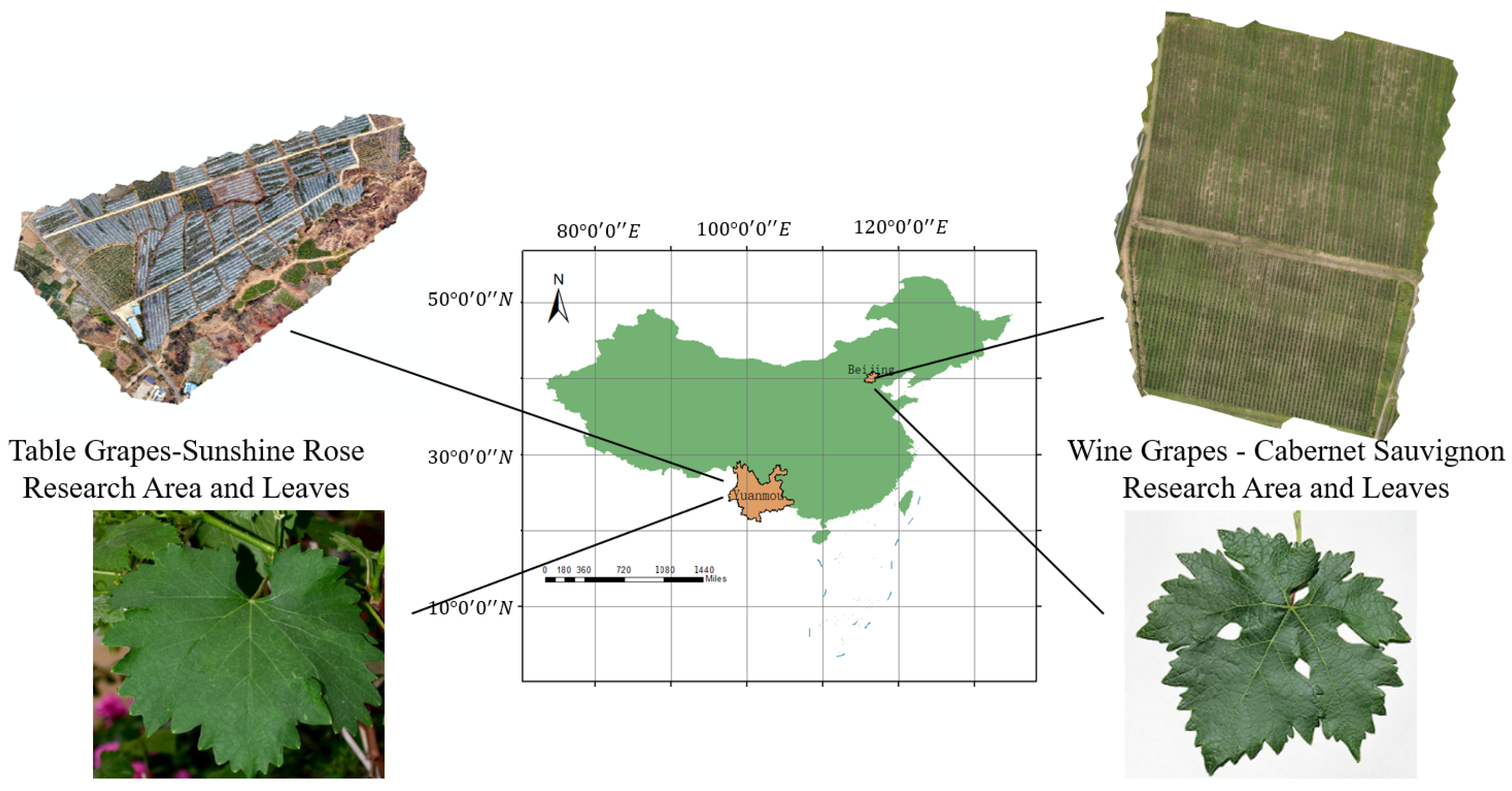
Figure 1. Geographical location of the study area.
Remotesensing 16 02174 g001
Figure 2. Random forest model principle.
Remotesensing 16 02174 g002
Figure 3. Raw spectral curves of grapevine leaves at different fertility stages.
Remotesensing 16 02174 g003
Figure 4. FOD spectral curve variation.
Remotesensing 16 02174 g004
Figure 5. (a) 0.1–1.0-order differential spectral curves. (b) 1.1–2.0-order differential spectral curves.
Remotesensing 16 02174 g005aRemotesensing 16 02174 g005b
Figure 6. (a) Correlation analysis of chlorophyll with spectral curves of all orders at different times. (b) Maximum and average values of correlation coefficients.
Remotesensing 16 02174 g006aRemotesensing 16 02174 g006b
Figure 7. Correlation analysis between vegetation index and chlorophyll content.
Remotesensing 16 02174 g007
Figure 8. (a) Scatterplot of LCC prediction model for ripening grapes. (b) Scatterplot of grape LCC prediction model during berry growing season. (c) Scatterplot of LCC prediction model for grapes at harvest time.
Remotesensing 16 02174 g008aRemotesensing 16 02174 g008b
Figure 9. Scatterplot of the LCC prediction model for grapes over the full life cycle.
Remotesensing 16 02174 g009
Table 1. Study area data information.
SiteTimeVarietyGrowing PeriodNumber of Neighborhoods
Fangshan District, Beijing19 August 2022Wine Grapes—Cabernet SauvignonRipening period32
Yuanmou County, Chuxiong Yi Autonomous Prefecture, Yunnan Province26 August 2023Edible Grapes—Sunshine RoseGrowing period30
4 November 2023Harvesting period29
Table 2. Area data information for the optimal number of orders for different periods.
All Reproductive PeriodsGrowing PeriodRipening PeriodHarvesting Period
Mean value/order(0.815) 0.7(0.848) 0.8(0.864) 0.8(0.773) 0.9
Max value/order(0.887) 1.0(0.908) 1.2(0.895) 0.8(0.874) 1.0
Table 3. Vegetation index calculation formula.
VIFormulaReferences
Anthocyanin reflectance index (ARI) 1 R 550 ( 1 R 700 ) [45]
Green carotenoid index (CAR_green) ( 1 R 510 1 R 550 ) × R 770 [46]
Chlorophyll absorption reflectance index (CARI) R 700 R 670 0.2 × ( R 700
R 550 )
[47]
Green chlorophyll index (CI_green) R 750 R 550 R 550 [46]
Red edge chlorophyll index (CI) R 750 R 705 R 705 [46]
Green normalized difference vegetation index (GNDVI) R 801 R 550 R 801 + R 550 [45]
Modified chlorophyll absorption reflectance index (MACRI) [ R 700 R 670 0.2
× ( R 700 R 550 ) ] × ( R 700
/ R 670 )
[48]
Modified normalized difference (mND_705) ( R 750 R 705 ) × ( R 750
+ R 705 2 R 445 ) 1
[49]
Modified simple ratio (mSR_705) ( R 750 R 445 ) × ( R 750
+ R 445 ) 1
[49]
Meris terrestrial chlorophyll index (MTCI) R 754 R 709 R 709 R 681 [50]
Normalized difference vegetation index (NDVI) R 800 R 680 R 800 + R 680 [51]
Red edge normalized difference vegetation index ( N D V I 705 ) R 750 R 705 R 750 + R 705 [52]
Normalized total pigment to chlorophyll index (NPCI) R 680 R 430 R 680 + R 430 [53]
Ratio vegetation index 1 ( R V I 1 ) R 765 R 720 [54]
Ratio vegetation index 2 ( R V I 2 ) R 740 R 720 [55]
Simple ratio (SR) R 800 R 680 [56]
Transformed chlorophyll absorption ratio (TCARI) 3 × [ R 700 R 670 0.2
× ( R 700 R 550 ) × ( R 700
/ R 670 ) ]
[57]
Transformed vegetation index (TVI) 0.5 × [ 120 × R 750 R 550
200 × ( R 670 R 550 ) ]
[58]
Table 4. Number of typical vegetation indices and maximum correlation coefficients.
Differential Order00.10.20.30.40.50.60.70.80.91.0
Number1312121412131313131312
Correlation coefficient0.7970.8070.8150.8220.8260.8260.8230.8310.8390.8470.856
Differential order1.11.21.31.41.51.61.71.81.92.0
Number10565443332
Correlation coefficient0.8610.8620.8520.8260.7750.7320.7080.6750.6340.579
Table 5. (a) Evaluation metrics for the grape LCC model during the ripe grapes. (b) Evaluation metrics for the grape LCC model during the berry growing season. (c) Evaluation metrics for LCC prediction model for harvested grapes.
(a)
Order R 2 RMSENRMSEOrder R 2 RMSENRMSE
Original0.6951.9754.6%1.10.7521.7834.1%
0.10.7281.8664.3%1.20.6822.0174.7%
0.20.7611.7494.1%1.30.6682.064.8%
0.30.7771.7164%1.40.6122.2285.2%
0.40.8241.4983.5%1.50.6911.9874.6%
0.50.8541.3653.2%1.60.6382.2075.1%
0.60.8641.3193.1%1.70.6232.3535.5%
0.70.8691.2953%1.80.5892.3415.7%
0.80.8831.2242.8%1.90.5282.3475.7%
0.90.8031.5863.7%2.00.4882.2595.4%
1.00.7891.6413.8%
(b)
Order R 2 RMSENRMSEOrder R 2 RMSENRMSE
Original0.6992.5345.6%1.10.6372.7996.2%
0.10.7012.55.5%1.20.7252.4215.4%
0.20.7172.4555.4%1.30.752.3065.1%
0.30.6932.5555.7%1.40.7022.5215.6%
0.40.7312.3935.3%1.50.7422.3455.2%
0.50.7372.3675.3%1.60.7482.3195.1%
0.60.7352.3755.3%1.70.7132.4725.5%
0.70.7612.2545%1.80.7522.2965.1%
0.80.7332.3835.3%1.90.6282.7986.1%
0.90.7532.2925.1%2.00.5763.4747.5%
1.00.6442.7526.1%
(c)
Order R 2 RMSENRMSEOrder R 2 RMSENRMSE
Original0.6312.24.6%1.10.7791.7043.6%
0.10.6482.154.5%1.20.7081.9574.1%
0.20.6991.9884.2%1.30.6192.2384.7%
0.30.6991.9874.2%1.40.6012.2894.8%
0.40.7491.8173.8%1.50.6842.0364.3%
0.50.7851.6793.5%1.60.6482.154.5%
0.60.8071.5933.3%1.70.6043.6177.7%
0.70.8041.6053.4%1.80.5693.497.8%
0.80.7811.6973.6%1.90.5872.5445.8%
0.90.7671.7483.7%2.00.5264.128.9%
1.00.7691.7423.7%
Table 6. Evaluation indexes of LCC prediction model for whole-birth grapevine.
Order R 2 RMSENRMSEOrder R 2 RMSENRMSE
Original0.6052.7996.2%1.10.6912.7465.5%
0.10.6882.4885.5%1.20.7632.1674.8%
0.20.7062.4125.4%1.30.7782.14.7%
0.30.7242.3375.2%1.40.7662.1534.8%
0.40.742.2695%1.50.7252.3355.2%
0.50.7222.3485.2%1.60.5942.8386.3%
0.60.7022.4265.4%1.70.552.9876.6%
0.70.6812.5135.6%1.80.5612.9516.5%
0.80.6312.7046%1.90.5193.3927.5%
0.90.6312.8036%2.00.4613.2687.3%
1.00.632.7096%
Disclaimer/Publisher’s Note: The statements, opinions and data contained in all publications are solely those of the individual author(s) and contributor(s) and not of MDPI and/or the editor(s). MDPI and/or the editor(s) disclaim responsibility for any injury to people or property resulting from any ideas, methods, instructions or products referred to in the content.