Article

Driving Factors and Trade-Offs/Synergies Analysis of the Spatiotemporal Changes of Multiple Ecosystem Services in the Han River Basin, China

1
College of Grassland Agriculture, Northwest A&F University, Xianyang 712100, China
2
State Key Laboratory of Soil Erosion and Dryland Farming on Loess Plateau, Institute of Soil and Water Conservation, Northwest A&F University, Xianyang 712100, China
3
College of Water Resources and Architectural Engineering, Northwest A&F University, Xianyang 712100, China
4
College of Mechanical and Electronic Engineering, Northwest A&F University, Xianyang 712100, China
*
Author to whom correspondence should be addressed.
Remote Sens. 2024, 16(12), 2115; https://doi.org/10.3390/rs16122115
Submission received: 22 March 2024 / Revised: 24 May 2024 / Accepted: 6 June 2024 / Published: 11 June 2024
(This article belongs to the Special Issue Assessment of Ecosystem Services Based on Satellite Data)

Abstract

:
Uncovering the trade-offs and synergy relationship of multiple ecosystem services (ESs) is important for scientific ecosystem management and the improvement of ecological service functions. In this study, we investigated the spatiotemporal changes of four typical ES types (i.e., water yield (WY), carbon storage (CS), soil conservation (SC), and habitat quality (HQ)) from 2001 to 2020 in the Han River Basin (HRB). Meanwhile, the trade-offs and synergies between paired ESs and the socioecological drivers of these ESs were further explored. The results showed that grassland, cropland, and bare land decreased by 12,141.3 km2, 624.09 km2, and 22.1 km2 during the study period, respectively, which can be attributed to their conversion to forests in the HRB. Temporally, the WY, CS, and SC all showed a continuously increasing trend. Spatially, WY and HQ exhibited bipolar clustering characteristics, with WY exhibiting low-value clustering in the upstream and high-value clustering in the downstream, while CS showed the clustering characteristics of a scattered distribution of cold and hot spots from 2001 to 2020. The spatial patterns of aggregation locations in CS and HQ were relatively similar, with clusters of higher ES values mainly distributed in the western and central regions and clusters of lower ES values mainly located in the eastern and southeastern regions, while the aggregation of WY was spatially concentrated. Overall, the CS showed a significant positive correlation with HQ, but a significant negative correlation with WY. Spatially, WY and HQ, CS, and SC showed a substantial trade-off relationship in the northwest and southeast parts of the study area, while HQ, CS, and SC mainly exhibited a synergistic relationship in most parts of the study area. Slope and temperature had high influencing factor coefficients on multiple ESs; the mixed effect of terrain and natural factors was significantly greater than the impact of a single factor on ESs, and terrain factors played an essential role in the changes in ESs. The findings can provide technical and theoretical support for integrated scientific ecosystem management and sustainable development at the local scale.

1. Introduction

Ecosystem services (ESs) are crucial for human production and livelihoods, as they provide necessary conditions that contribute to human health, well-being, and the overall functioning of societies. These services encompass four major functions, namely provisioning, culture, support, and regulation [1]. Among the numerous ESs, water yield (WY), soil conservation (SC), carbon storage (CS), and habitat quality (HQ) are of great concern. In recent years, industrialization has accelerated changes in ecosystem structures. This, coupled with the overuse of ecological resources, has degraded vital ecological functions. Manifestations of this degradation include air pollution, soil erosion, reduced biodiversity, and significant eutrophication of water bodies, all of which profoundly impact human life [2,3]. Furthermore, due to the intertwined effects of complex climate change and human activities, various types of ESs will demonstrate both conflicting trade-offs and synergistic relationships [4,5]. Specifically, multiple ESs do not exist independently, but rather have a trade-off state of increasing and decreasing or a synergistic state of increasing and decreasing simultaneously [6]. These trade-offs and synergistic relationships are influenced by land-use type change, climate change, and human activity [3,7,8,9]. Consequently, quantifying how these typical ESs change and interact with each other under different environmental conditions is crucial for developing ecological plans and managing ecosystems by government departments.
In recent years, as a comprehensive interdisciplinary discipline hot spot, ESs are gradually being implemented from theoretical research to practical applications [10]. At present, research on ESs includes analysis of spatiotemporal changes and the trade-off/synergy of multiple ESs and ES bundles. For instance, Geng, Li, Zhang, Yang, Jing and Rong [4] quantitatively evaluated food production, WY, and SC in the Yellow River Basin of China and found that these ESs exhibited synergistic relationships in most regions, while only trade-off relationships were present on a local scale. Scholars have employed diverse methodologies to examine the trade-offs and synergies of ESs across various scales and regions. For example, most studies use ordinary correlation analysis to reveal the correlation between different ecosystem services [11,12,13]. However, due to the significant spatial heterogeneity in the trade-off synergy between different ESs, relying solely on correlation coefficients cannot reveal the trade-off synergy between different ESs at the spatial scale. Therefore, accurately identifying the trade-offs between different ESs at the spatial scale can provide decision-makers with more accurate spatial decision-making references for ecosystem management. Moreover, the spatial heterogeneity of natural and socio-economic factors leads to a distinct spatial variability in the trade-offs and synergies of ESs. Consequently, Geographically Weighted Regression (GWR) and bivariate spatial autocorrelation analysis are commonly employed to examine the spatial patterns in trade-offs and synergies among various ESs [14,15,16,17]. For the identification of ES bundles, k-means clustering analysis, self-organizing maps (SOMs), and the structural equation model are common methods [18,19,20].
ESs have proven to be significantly influenced by climate factors such as rainfall and temperature, and socio-economic factors are also considered important driving factors of ESs [11,13,21], especially for land-use change related to human activities [8,22]. Recent studies have primarily focused on the influence of natural factors, including temperature, precipitation, evapotranspiration, and topography, on ES changes [7,11,23], Additionally, previous studies also examined the impact of socio-economic factors on ESs [4,5]. The Han River Basin (HRB) serves as the water source for the Middle Route of the South-to-North Water Transfer Project, a large-scale cross-basin water transfer initiative, annually transporting approximately 10 billion cubic meters of water to northern cities [8,24]. The HRB is crucial for reconstructing China’s water network and allocating its water resources. However, the HRB’s socio-economic development, increasing water use, and water diversion impacts have significantly pressured the watershed’s ecosystem, affecting sustainable socio-economic development and the ecological environment [25]. Many scholars have studied the ecological environment changes and hydrological characteristics in the HRB, such as vegetation ecosystem patterns [26] and runoff change [24,27]. However, the spatiotemporal pattern evolution of various ecosystem functional characteristics such as WY, SC, CS, and HQ has not been studied. Additionally, the trade-offs and synergies among these typical ES functions, along with their key driving factors, remain unexplored [28]. Scientific exploration of the WY, SC, CS, and HQ functions of ecosystems can significantly contribute to regional climate change mitigation, ecological management, and species diversity enhancement.
We selected the HRB as our study area to analyze the spatiotemporal changes of multiple ESs and the trade-offs/synergies interactions and social-ecological driving factors among these multiple ESs and further identify the ES bundles (ESBs) from 2001 to 2020. This study aimed to (1) investigate the spatiotemporal dynamics of WY, CS, SC, and HQ, and identify these ES hot spots during the study period; (2) examine the trade-offs and synergistic relationships between multiple ESs at grid scales from 2001 to 2020; (3) identify the changes in ESBs of multiple ESs; and (4) clarify how various socio-ecological factors have driven changes in ESs and their interrelationships in the study area. Our findings offer insights into the management of the local ecosystem and inform the development of ecological restoration strategies to enhance ecological service functions.

2. Materials and Methods

2.1. Study Area

The Han River is the longest tributary of the Yangtze River, located at 106°51′E to 107°10′E and 33°02′N to 33°22′N. The Han River originates from the southern foot of the Qinling Mountains in Ningqiang County, Hanzhong City, Shaanxi Province, with a total length of 1577 km. The total area of the Han River Basin (HRB) is 159,000 km2, and the basin involves 20 districts (cities) and 78 counties (cities) in 5 provinces and cities (Hubei, Shaanxi, Sichuan, Chongqing, and Gansu) (Figure 1a). The topography of the HRB is high in the northwest and low in the southeast (Figure 1b). The geological structure is roughly bounded by Xichuan-Danjiangkou-Nanzhang, with folded uplifted low mountainous areas in the west and plains and hills in the east. The HRB is located in the subtropical monsoon region and experiences a mild, humid climate with an annual average precipitation ranging from 700 to 1100 mm. In the HRB, the temperature difference between the upper and lower reaches is minimal, characterized by warm winters, hot summers, and an average temperature exceeding 22 °C. The HRB’s land use shows significant topographic and geographical variation, primarily comprising forests, croplands, and grasslands, followed by urban areas, wetlands, water bodies, and bare land (Figure 1c). The Han River is the main water source of the Middle Route Project of the South-to-North Water Transfer. With the opening of the Middle Route Project of the South-to-North Water Transfer and the acceleration of urbanization, the ecosystem has been affected to varying degrees in the HRB, especially ecological functions such as WS, SC, and HQ, which are constantly changing. Meanwhile, to protect the HRB’s ecological environment, the government has implemented a series of ecological restoration and protection projects, including natural forest protection and farmland conversion into forests.

2.2. Data Sources and Processing

The datasets used in this study include satellite imagery datasets, land use/cover datasets, meteorological datasets, topography data (elevation and slope), and other related ancillary datasets (Table 1). The Land use/cover data in 2001, 2005, 2010, 2015, and 2020 were obtained from the MCD12Q1 dataset (https://search.earthdata.nasa.gov/search, accessed on 1 October 2023), with a resolution of 500 m, which were reclassified into 6 categories (forest, grassland, cropland, wetland, urban land, and unused land). The meteorological data from 2001 to 2020 including temperature, precipitation, evapotranspiration, and potential evapotranspiration were collected from the Loess Plateau Science Data Center, National Earth System Science Data Sharing Infrastructure, National Science & Technology Infrastructure of China (http://loess.geodata.cn, accessed on 21 March 2024), with a resolution of 500 m. The Enhanced vegetation index (EVI) data with a resolution of 500 m from 2001 to 2020 were available from https://earthengine.google.com/, accessed on 21 March 2024. The Digital Elevation Mode (DEM) data with a resolution of 90 m were derived from SRTMDEM of the China Geospatial Data Cloud. We extracted the elevation, slope aspects, and slope gradients of the study area based on DEM data. The Nighttime Light data at a spatial resolution of 1 km were obtained from the NOAA website’s NGDC data center (https://www.ngdc.noaa.gov/eog/download.html, accessed on 21 March 2024). The population grid datasets from 2001 to 2020 were collected from World Pop (https://www.worldpop.org/project/list, accessed on 21 March 2024). The spatial resolution was set at 1 km. To ensure consistency across all data, we resampled all raster data to a 1 km resolution using ArcGIS 10.8.

2.3. Quantification of ESs

In this study, four ESs—carbon storage (CS), soil conservation (SC), water yield (WY), and habitat quality (HQ)—were selected based on the Millennium Ecosystem Assessment and the Common International Classification of Ecosystem Services version 5.1 [1]. All four ESs were quantitatively evaluated by the InVEST model (Integrated Valuation of Ecosystem Services and Tradeoffs), which is an ecosystem service application tool developed in 2007 by Stanford University, the Worldwide Fund for Nature and The Nature Conservancy (InVEST 3.14.1 User’s Guide).

2.3.1. Quantification of Water Yield (WY)

The water yield (WY) service was estimated using the InVEST model, based on water balance principles and Budyko’s coupled hydrothermal balance assumption, calculating the difference between precipitation and actual evapotranspiration in various grid cells [29]. The description of the WY service is as follows:
Y ( x ) = ( 1 A E T x P x ) × P x
A E T x P x = 1 + P E T ( x ) P ( x ) 1 + P E T ( x ) P ( x ) W 1 W
P E T ( x ) = K c ( x ) × E T 0 ( x )
W ( x ) = A W C ( x ) × Z P ( x ) + 1.25
where Yx is the annual WY (mm); AETx and Px represent the annual actual evapotranspiration (mm) and annual precipitation (mm), respectively; PETx is the potential evapotranspiration (mm); Kcx is the vegetation crop evapotranspiration coefficient; ET0x denotes the reference evapotranspiration; Wx is defined by the ratio of annual plant water demand to annual precipitation (dimensionless); and AWCx is the effective soil water content (mm). The vegetation evapotranspiration coefficient was taken in the range of 0–1.5. The maximum rooting depth of vegetation was calculated based on the World Soil Database.

2.3.2. Quantification of Carbon Storage (CS)

We utilized the InVEST model to estimate the carbon storage (CS) in various ecosystems. The InVEST model calculations were based on four types of carbon pools: above-ground, below-ground, soil organic, and dead organic matter carbon pools [30]. The formulas used are as follows:
C s = C a b o v e + C b e l o w + C s o i l + C d e a d
where Cs represents the total carbon stock (t/hm2); Cabove is the biogenic carbon stock in the above-ground part; Cbelow is the biogenic carbon stock in the below-ground part; Csoil and Cdead represent the soil organic carbon stock and the dead organic matter carbon stock, respectively. The carbon density data of different land types considered in this study were mainly obtained from the National Ecological Science Data Center (http://www.cnem.org.cn/, accessed on 21 March 2024).

2.3.3. Quantification of Habitat Quality (HQ)

Habitat Quality actually refers to the potential of an ecosystem to provide the necessary conditions for species to survive and reproduce, which is reflected by the Habitat Quality Index. The core of this method is to establish a connection between habitat quality and threat sources, that is, by calculating the negative impact of threat sources on the habitat, the degree of habitat degradation is obtained, and then habitat quality is calculated based on the suitability and degree of degradation of the habitat [31]. The data required for specific calculations include threat types, the maximum distance that each threat affects habitat quality, the impact index of each threat on habitat quality, and the spatial attenuation type of each threat. This is calculated using the Habitat Quality module of the InVEST model, which was expressed by the following formula:
Q x j = H j 1 D x j Z / D x j Z + k Z
where Qxj is the HQ of grid x in the land-use/cover type j; Hj refers to the habitat suitability of the land-use/cover type j; Dxj is the level of habitat threat to grid x in the land-use/cover type j; k is a half-saturation constant (0.5); and z is a normalization constant (2.5).

2.3.4. Quantification of Soil Conservation (SC)

Soil conservation is defined as an ecosystem’s capacity to regulate erosion, thereby preventing soil loss through its structures and processes and retaining and storing sediment. SC was calculated using the Modified Universal Soil Loss Equation (RUSLE) and the SC module in the InVEST model, which determines the difference between potential and actual soil erosion [32]. The specific calculation formulas are as follows [33]:
R K L S x = R x × K x × L S x
U L S E x = R x × K x × L S x × C x × P x
S E D R E T x = R K L S x U S L E x
where S E D R E T x is the soil conservation amount of the grid x ; R K L S x is the potential soil erosion amount of grid x ; U S L E x is the actual soil erosion amount of grid x ; R x is the rainfall erosion force factor; K x is the soil erodibility factor; L S x is the slope and slope length factor; C x is the vegetation cover factor; and P x is the soil and water conservation measure factor. Equation (7) is the potential soil erosion without considering the vegetation factor and management measures, and Equation (8) is the actual soil erosion under the condition of considering the vegetation factor and management measures.

2.4. Spatial Autocorrelation and Hot Spot Analysis of ESs

We applied the Global Moran’s I index to analyze the spatial autocorrelation of ESs and assess their aggregation degree in the HRB. The index is expressed as follows:
M o r a n s   I = n i = 1 n j = 1 n w i j x i x ¯ x j x ¯ i = 1 n x i x ¯ 2 i j w i j
where I is the Moran index; n is the number of spatial grid cells; x i and x j represent the observed value of spatial cell i and spatial cell j, respectively; x i x ¯ refers to the deviation of the observed value on the ith spatial cell from the mean value; and w i j is the spatial weight matrix of grids i and j [34].
To examine the spatial aggregation of various ecosystem service (ES) functions in the HRB, we employed the Getis-Ord Gi* statistical index, a hot spot analysis tool in ArcGIS, to identify cold and hot spots in the study area. ES hot spots and cold spots were identified using p-values and z-scores, with statistical significance defined at the 95% confidence level (p < 0.05). Spatial clustering was considered significant when z-scores exceeded 1.64 in absolute value. Higher z-scores indicated clusters of higher ES values (hot spots), while lower z-scores pointed to clusters with lower ES values (cold spots).
G i = j = 1 n w i j x j j = 1 n x j
Z ( G i ) = j = 1 n w i j x j x ¯ j = 1 n w i j S n j = 1 n w i j 2 j = 1 n w i j 2 n 1
S = j = 1 n x j 2 n 1 x ¯ 2
where G i is the agglomeration index of patch i; Wij is the spatial weight matrix between patches i and j. For ease of interpretation, Wij may be in row standardized form, though this is not necessary, and by convention, Wii = 0 [35]; xi and xj present the attribute values of patches i and j; n is the total number of patches; x ¯ is the mean value of all patches; S is the standard deviation of the attribute values of all patches. The Z-value is the score of G i and the p value is a probability. Specifically, a higher Z value and a smaller p value indicate a more obvious clustering of hot spots, while a smaller Z value and a smaller p value imply a more obvious clustering of cold spots [7].

2.5. Analyses of Trade-Offs/Synergies among ESs

In this study, we conducted correlation analysis to explore the trade-offs and synergies among various ESs. Specifically, we utilized the ‘corrplot’ package in R4.3.2 software for Spearman’s correlation analysis, covering five years: 2001, 2005, 2010, 2015, and 2020. Specifically, a positive correlation coefficient between ES pairs, significant at the 0.05 (or 0.01) level, indicated a synergistic (or significantly synergistic) relationship, and vice versa. The spatial distribution maps depicting trade-offs and synergies among various ESs were created using ArcMap 10.8 software.

2.6. Identification of ES Bundles (ESBs)

The ES bundle is a series of ecosystem services that repeatedly appear in space and time [36]. The concept of an ecosystem service bundle can identify the dominant services in a region. In the ecosystem service bundle, some services have dependency relationships and occur simultaneously, while others grow and disappear. This can analyze the trade-offs and synergies between multiple ecosystem services [37] and improve the management level of multifunctional landscapes. Bundle analysis of multiple ecosystem services yields the “class” of the ecosystem service cluster in the study area. The analysis of ecosystem service bundles helps to understand the spatial distribution of different services and clarify the location of the trade-offs and synergies between ecosystem services.
We used SOM to identify grid-scale ES bundles [20]. Specifically, by measuring the similarity between different ESs, the spatial cells with higher similarity were divided into the same ES clusters, and spatial cells with higher dissimilarity were divided into different ES clusters for functional partitioning of ESs. Each grid was categorized into an ES bundle based on the spatial co-occurrence similarity of ES. In this study, we employed the ‘raster’, ‘rgdal’, ‘ggradar’, ‘tibble’, and ‘stars’ packages in R4.3.2 software for spatial clustering of ES and functional partitioning.

2.7. Model of Geographical Detector

In this study, we selected 8 variables as potential drivers of ESs, including socioeconomic factors (population density and nighttime light index), climate and vegetation factors (EVI, mean annual temperature, mean annual precipitation, and evapotranspiration), and topographic factors (slope orientation and slope) as independent variables. We utilized the factor detector panel in the geographical detector to ascertain the relationships between independent variables and dependent ESs. Meanwhile, we employed the interaction detector panel to assess the magnitude of interaction effect coefficients for each driving factor on the ESs.

3. Results

3.1. Land Use Change in the HRB

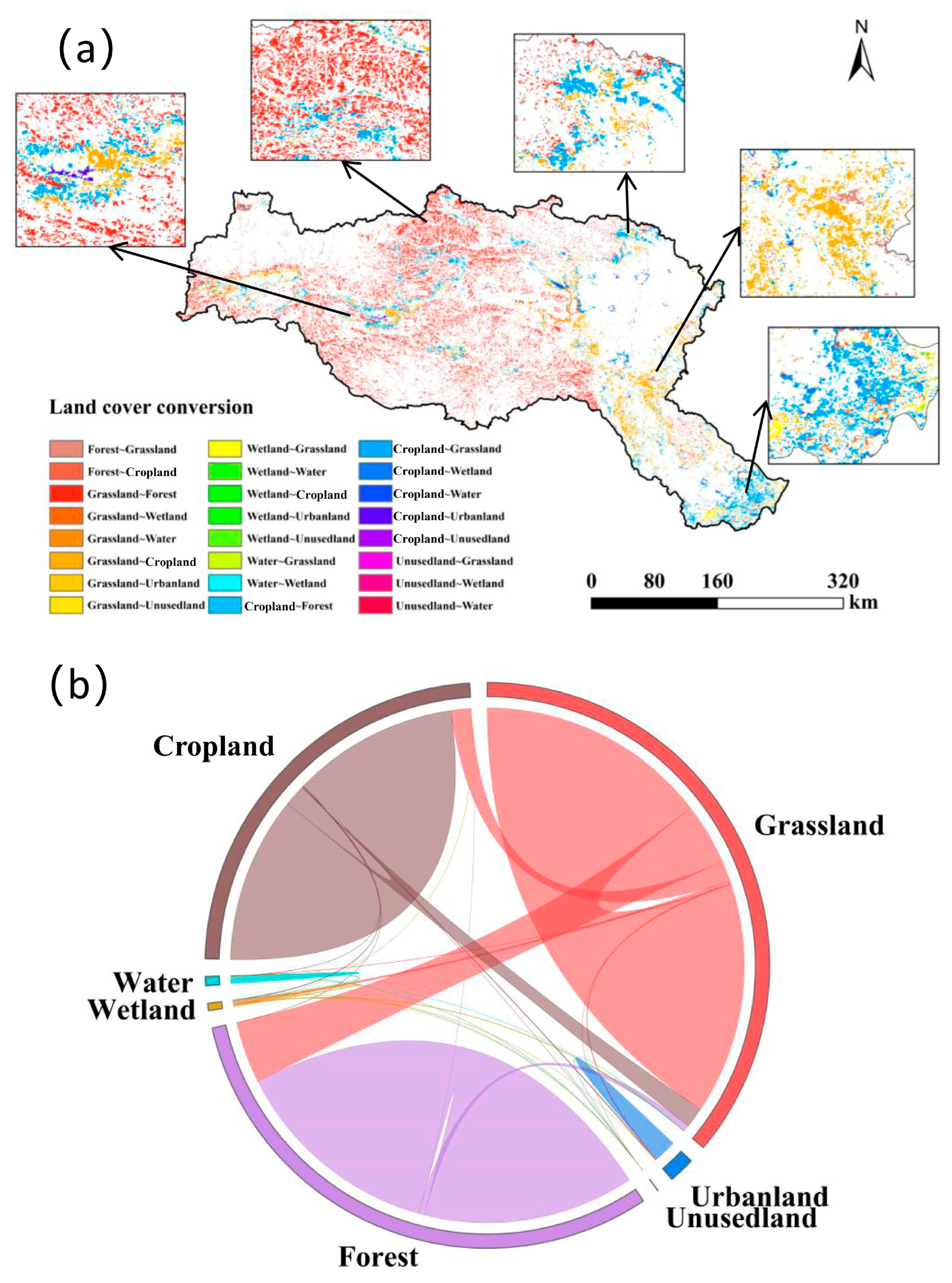
The land-use change characteristics in the HRB between 2001 and 2020 are shown in Table 2 and Figure 2. Forest, grassland, and cropland were the dominant land-use types in the HRB, which accounted for more than 97% of the total study area. During the past 20 years, the areas of different land-use types have changed, with the areas of grassland, bare land, and cropland decreasing, and the urban land, forests, water bodies, and wetlands increasing. Specifically, the grassland area decreased by 12,141.3 km2 (18.27%). Meanwhile, the area of arable land and bare land decreased by 624.09 km2 (1.57%) and 22.1 km2 (66.07%), respectively, while the forest area increased by 11,732.1 km2 (25.76%). These changes are attributable to the implementation of the policy that converts cropland into forests and grasslands. In addition, the area of urban land, water bodies, and wetlands increased by 407.2 km2 (17.5%), 162.36 km2 (20.77%), and 485.85 km2 (106.77%), respectively, which were consistent with the economic and social development trend and urbanization process in the HRB. Figure 2b also showed that all land use types had transformed. Specifically, nearly 19.44% (12,918.44 km2) of grassland was converted to forest during the 20 years, and a relatively small proportion of forest was converted to grassland and cropland (2.68%), while a larger area of cropland (4445.4 km2) was converted to forest and grassland. Moreover, the area of urban land increased obviously. Overall, the changes in arable land, forest, grassland, and urban land were obvious and showed a large spatial heterogeneity during 2001–2020, which might have a serious impact on the distribution and dynamics of ESs in the HRB.

3.2. ES Patterns in the HRB

3.2.1. Spatial and Temporal Changes in ESs

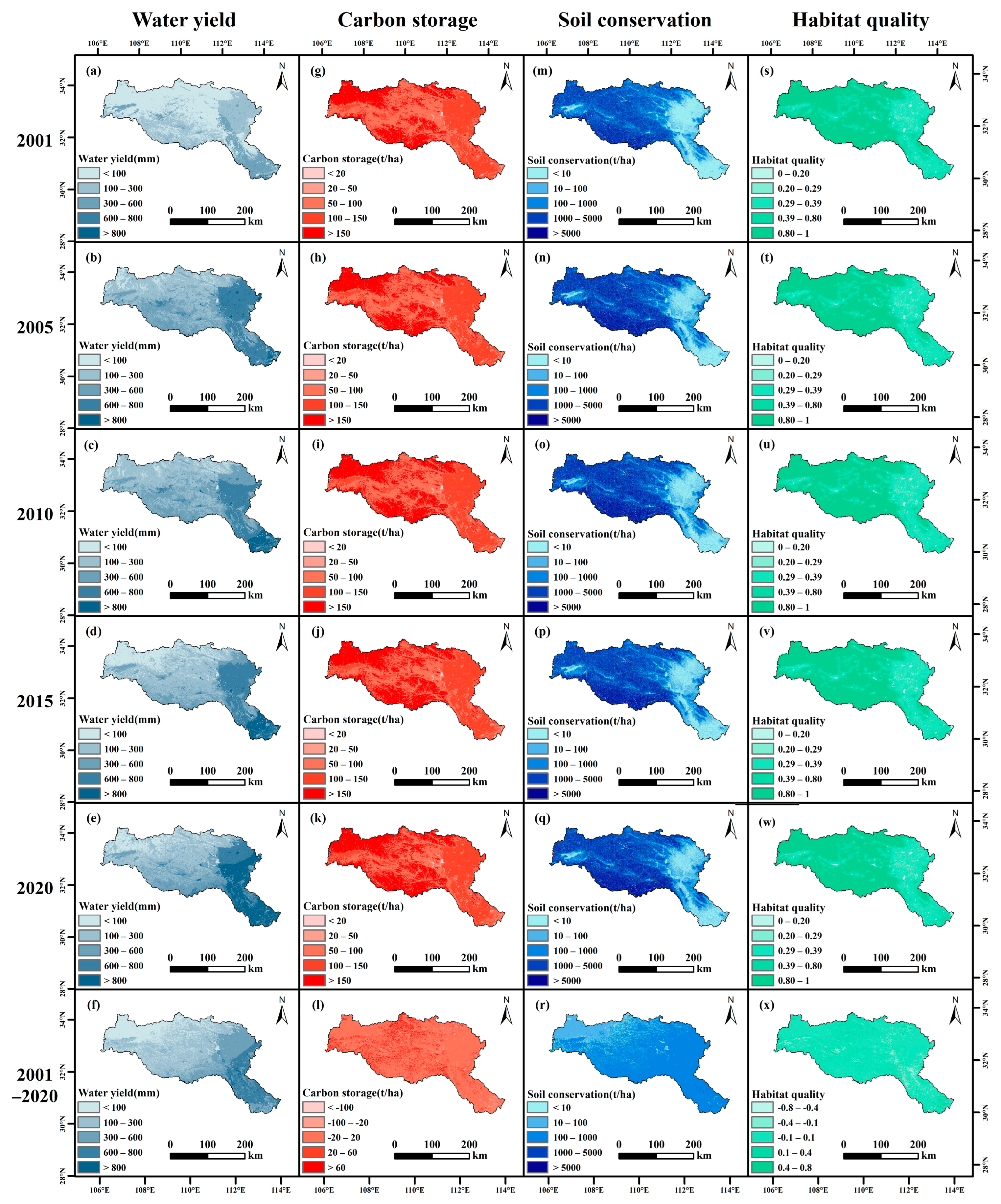
The spatial patterns and changes in ESs in the HRB from 2001 to 2020 are shown in Figure 3. As shown in Figure 3a–f, WY exhibited fluctuating changes between 2001 and 2020. In the period from 2001 to 2005, increased WY was observed in an area encompassing 99.13% of the HRB, primarily located in the southern area of the HRB and Nanyang City. During 2005–2010 and 2010–2015, the area with decreased WY expanded, accounting for 40.64% and 66.09% of the total area, respectively, which was mainly concentrated in Nanyang and Yicheng City. From 2015 to 2020, the region with increased WY covered 96.96% of the total area, primarily situated downstream of Danjiangkou. Over the course of 20 years, the northern part of the HRB maintained a relatively stable WY, consistently below 200 mm. Based on the spatial distribution and variation characteristics of CS (Figure 3g–l), the changes in CS were relatively apparent in the HRB between 2001 and 2020, primarily concentrated in the upstream area of Danjiangkou, with the most significant increase occurring in urban land. Spatially, it typically followed a pattern of higher CS in the western mountainous regions and lower storage in the eastern hills. Specifically, the regions with higher CS were mainly located in the northern and southern regions of the upstream mountainous areas, which was closely associated with the distribution of vegetation patterns. Specifically, forests predominantly occupied areas with high CS values, whereas grasslands and bare land dominated low CS values. In terms of SC, the total SC capacity of the HRB showed a steadily increasing trend over time. The Cropland area had relatively poor SC capacity in the eastern part of the HRB. Nevertheless, the SC capacity gradually increased due to the conversion of cropland to other land use types between 2001 and 2020. Regions with higher SC levels were predominantly located in the central and southern areas of the HRB. In addition, there was no significant change in SC in forest and urban areas (Figure 3m–r). For HQ (Figure 3s–x), it was found that the area with increased HQ was relatively small from 2001 to 2005 in the HRB, occupying only 13.89% of the total area. However, there was an obvious increase in HQ during the periods of 2005–2010 and 2010–2015, accounting for 24.48% and 26.59% of the total area, respectively. Subsequently, there was a decline in the proportion exhibiting increased habitat quality from 2015 to 2020, which was reduced to 24.32%. Overall, most of the areas with an increased HQ index were also found around the cities of the study area.
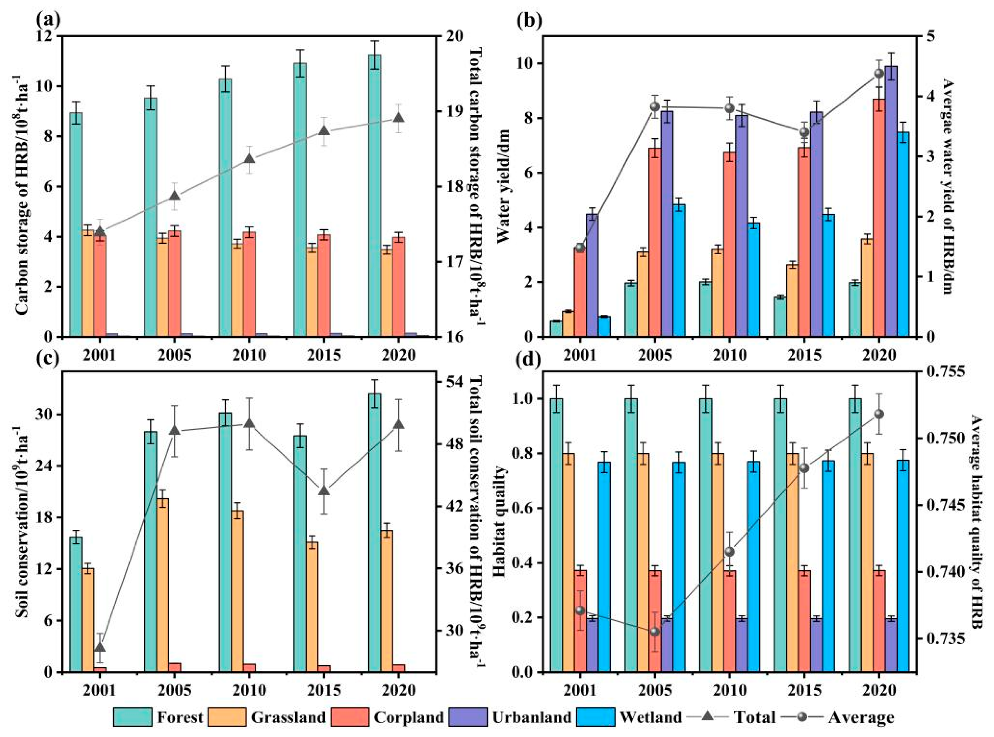
The inter-annual variation characteristics of ES values of different land types in the HRB from 2001 to 2020 are presented in Figure 4. From 2001–2020, the average WY exhibited a fluctuating increasing trend in the HRB, with an average growth rate of 17.46 mm/a. The multi-year average WY was 337.69 mm. Among the representative years (2001, 2005, 2010, 2015, and 2020), the average WY was 147.56 mm, 382.61 mm, 380.1 mm, 340.28 mm, and 437.911 mm, respectively. Notably, WY experienced a significantly increasing trend with a change of 235.051 mm from 2001 to 2005. Although there was a slight decline in the growth rate of WY from 2005 to 2015, the WY exhibited another increasing trend from 2015 to 2020. Among various land-use types, wetlands showed the most significant increase in water yield, increasing from 74.44 mm in 2001 to 748.26 mm in 2020. Conversely, the WY proportions for forestland and grassland experienced a slight increase, increasing from 5.77% and 9.39% in 2001 to 6.25% and 11.33% in 2020, respectively. In addition, the WY proportions for croplands and urban areas displayed an obviously decreasing trend, decreasing from 32.54% and 44.86% in 2001 to 27.48% and 31.28% in 2020, respectively. The total CS in the HRB during the five representative years was 283.13 × 10⁹ t, 492.28 × 10⁹ t, 499.17 × 10⁹ t, 434.02 × 10⁹ t, and 498.10 × 10⁹ t, indicating a significant overall upward trend. The proportion of forestland CS increased from 51.4% to 59.48%, whereas the proportion and variation of CS in urban land and wetlands were relatively small. Conversely, the proportion of total CS in grassland decreased from 24.46% to 18.4%, whereas the proportion of CS in cropland only had a gradual decrease from 23.21% to 21.02%. In the five representative years, the total SC amounts were 83.13 × 10⁹ t, 492.28 × 10⁹ t, 499.17 × 10⁹ t, 434.02 × 10⁹ t, and 498.10 × 10⁹ t, showing an overall fluctuating growth trend. Specifically, the SC amounts remained stable from 2005 to 2010 and slightly declined from 2010 to 2015, and then experienced an increase again from 2015 to 2020. The proportions of SC changes across different land-use types were similar. The SC proportions of forestland, urban land, and wetland had been continuously increasing, while the SC proportions of grassland and cropland had been decreasing. The average HQ of the HRB in the five representative years was 0.737, 0.736, 0.742, 0.748, and 0.752, respectively. Specifically, the average growth rate of HQ was 0.0009/a, indicating an overall increasing trend with fluctuations. From 2001 to 2015, the HQ was below the average value of 0.74.

3.2.2. Global Spatial Autocorrelation of ESs

The Global Moran’s I, Getis-Ord General G, and Z-scores were calculated to assess the spatial autocorrelation of ESs (Table 3). Additionally, the observed values for General G exceeded the expected values (p < 0.001), signifying a tendency of the ESs to cluster around high values. Specifically, the global Moran’s I value for WY increased from 0.58 to 0.76, indicating a significant increase in the clustering of WY values. The values for estimated and expected General G remained unchanged, suggesting that the correlation of high values remained constant. The Moran’s I value for CS decreased from 0.57 to 0.45, indicating a significant decrease in the clustering of CS. The difference between estimated and expected General G decreased, indicating a reduction in the correlation of high-value data. The global Moran’s I value for SC increased slightly from 0.14 to 0.15, indicating a slight increase in the clustering of SC. The values for estimated and expected General G remained unchanged, suggesting that the correlation of high-value data remained constant. The global Moran’s I value for HQ varied from 0.47 to 0.28, indicating a significant change in the clustering of HQ. The values for estimated and expected General G slightly decreased, indicating a reduction in the correlation of high-value data. Moreover, the Moran’s I values of all ES during the study period were statistically significant at a 99% confidence level (Z (I) > 2.58), indicating significant spatial correlation. Based on this, further research on a more complex spatial correlation of ES results can be conducted.

3.2.3. The Cold Hot Spots of ESs

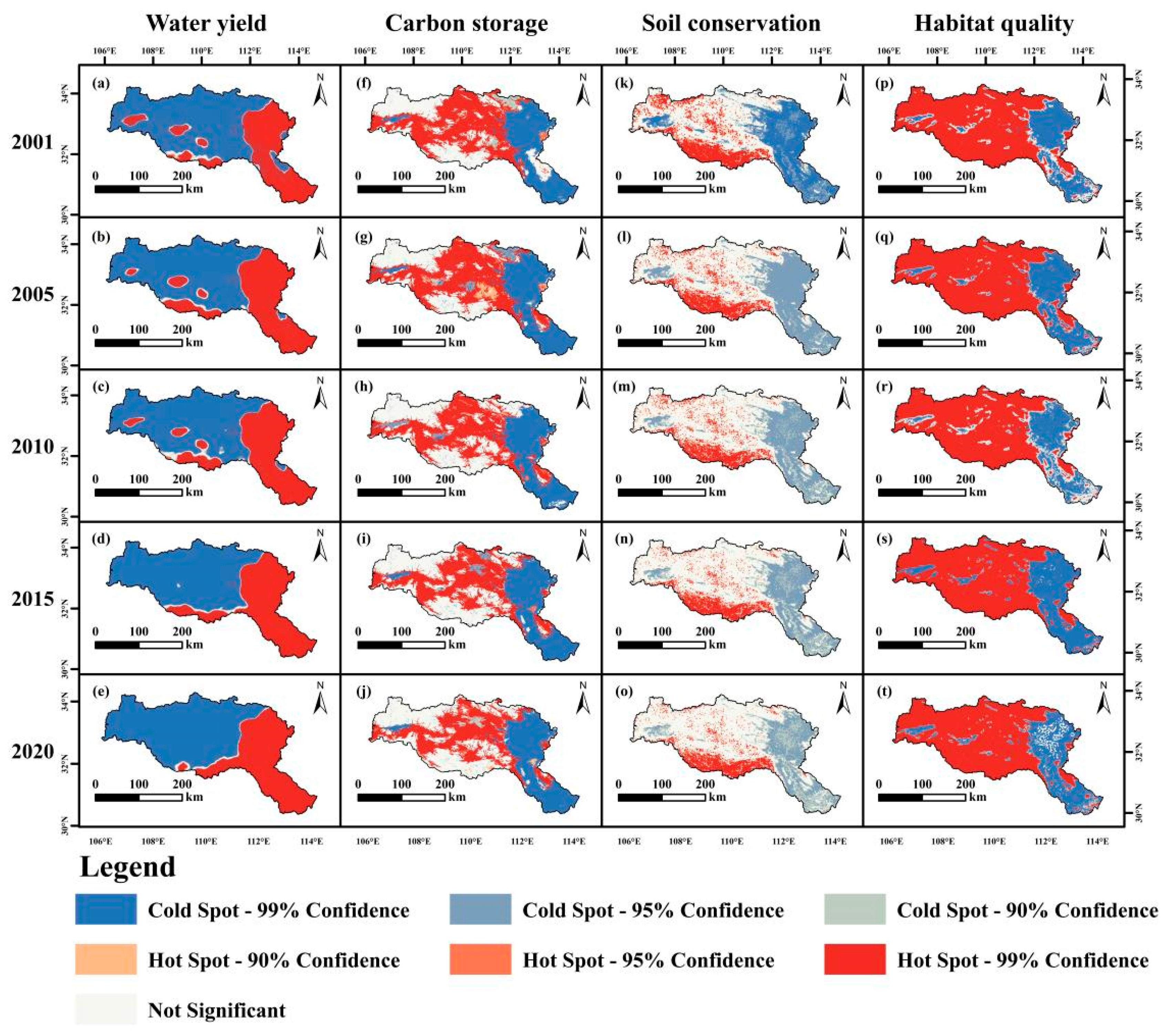
The spatial patterns of the cold hot spots of WY, CS, SC, and HQ in the HRB from 2001 to 2020 were mapped using the Gi* hot spot analysis (Figure 5). In relation to WY, a distinct spatial distribution pattern was observed, with cold spots clustered in the west and hot spots in the east. Sporadic hot spot clusters were identified in the western cities and their surrounding areas between 2001 and 2015. However, these clusters disappeared after 2015. Similarly, CS and HQ exhibited similar spatial distributions of hot and cold spots. Most of the region was characterized by hot spot clusters for CS in the west and cold spot clusters in the east. A decreasing trend in hot spot clusters for CS was observed in the western regions. Conversely, insignificant hot and cold spot clusters were observed in the southwest region of Da Hongshan in 2001, and these cold spot clusters gradually transformed into hot spot clusters from 2005 to 2020. The distribution of cold and hot spots for HQ displayed a clustering of cold spots surrounding the western cities. Additionally, the degree of cold spot clustering of HQ decreased annually in the eastern regions from 2001 to 2010. After a slight increase in 2015, the degree of cold spot clustering of HQ declined again in the eastern regions in 2020. The overall SC pattern revealed hot spot clusters in the south and cold spot clusters in the east, alongside significant hot and cold spot clusters in the central and northern regions. The distribution of SC’s cold and hot spots remained relatively stable. From 2001 to 2005, the degree of SC clustering decreased in some hot spot areas of the central and northern regions. Moreover, the extreme cold spot cluster of SC transformed into a cold spot cluster in the east area, and the cold spot cluster of SC gradually transitioned into an insignificant cold spot in the eastern area after 2005.

3.3. Trade-Off and Synergy between ESs

3.3.1. Correlation Analysis

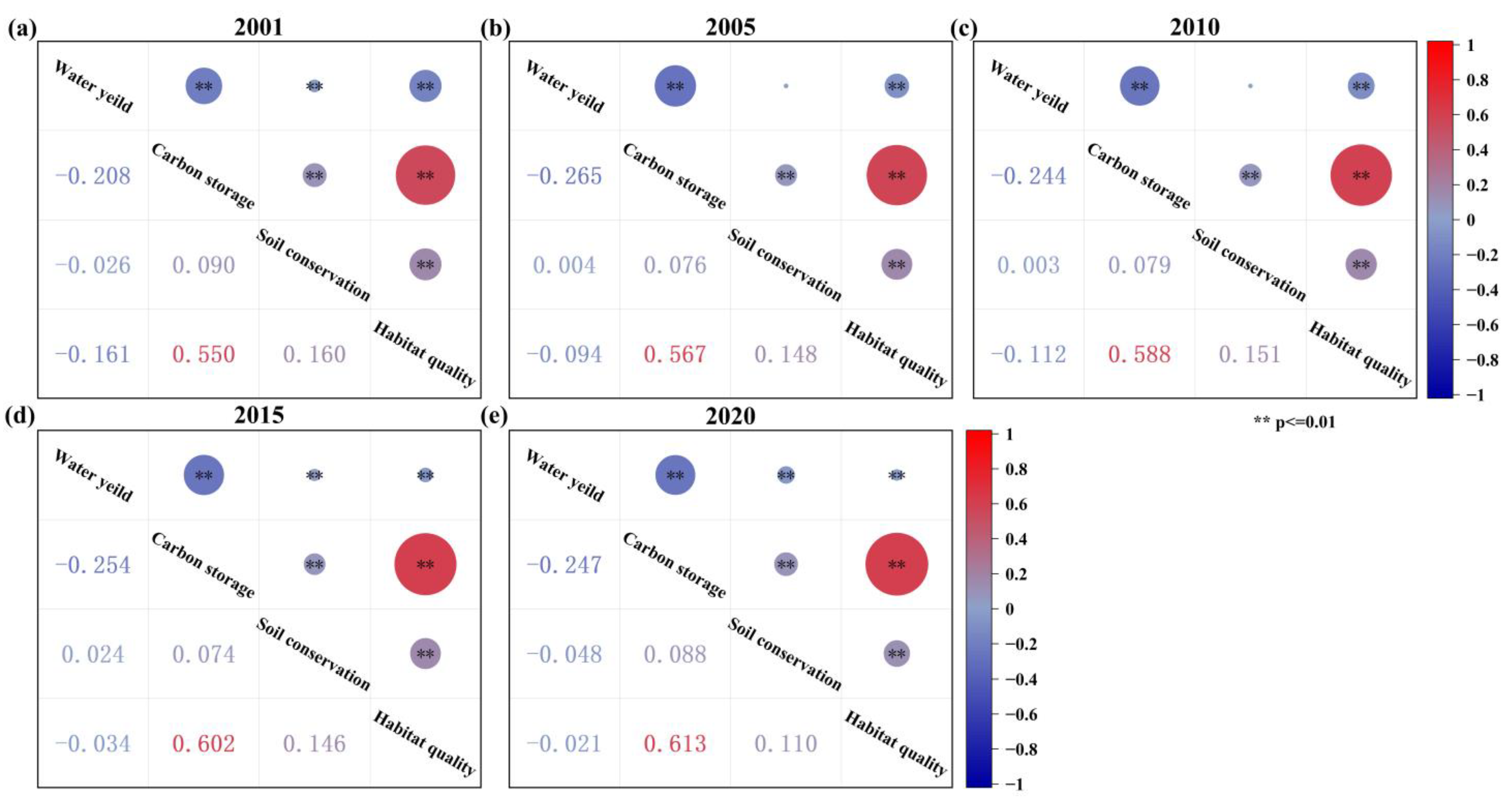
The relationships among four ESs were analyzed using Spearman correlation results, identifying six significant correlations among them (Figure 6). All correlations between the ES pairs were statistically significant (p < 0.05) (Figure 6). The correlations across these five representative years were relatively similar. Specifically, a clear positive correlation between HQ and CS and a clear negative correlation between WY and CS were observed in these five representative years, while the other correlations were relatively weak.
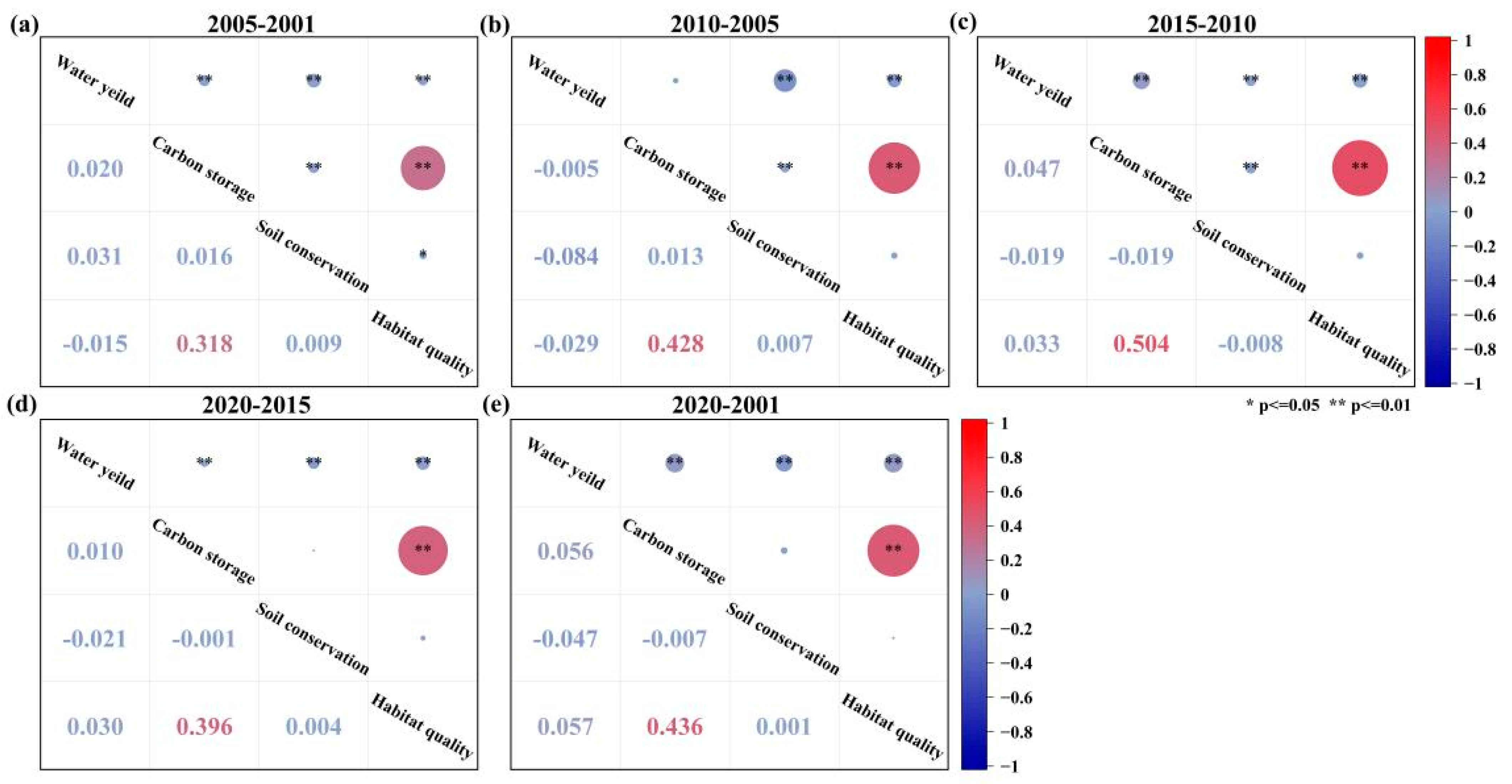
In addition, to further explore the correlations among the four ESs, another Spearman correlation result analysis was performed on the ES results of the interannual variation of the five years, and four significant correlations (p < 0.05) were identified (Figure 7). As shown in Figure 7, there was no correlation between HQ and SC or SC and CS except for a weak correlation during the periods of 2001–2005 and 2005–2010. Moreover, the interannual variation correlation between HQ and CS showed a slow increasing trend, while the other three correlations continued to show weak correlations.

3.3.2. Trade-Off and Synergy between Ecosystem Services

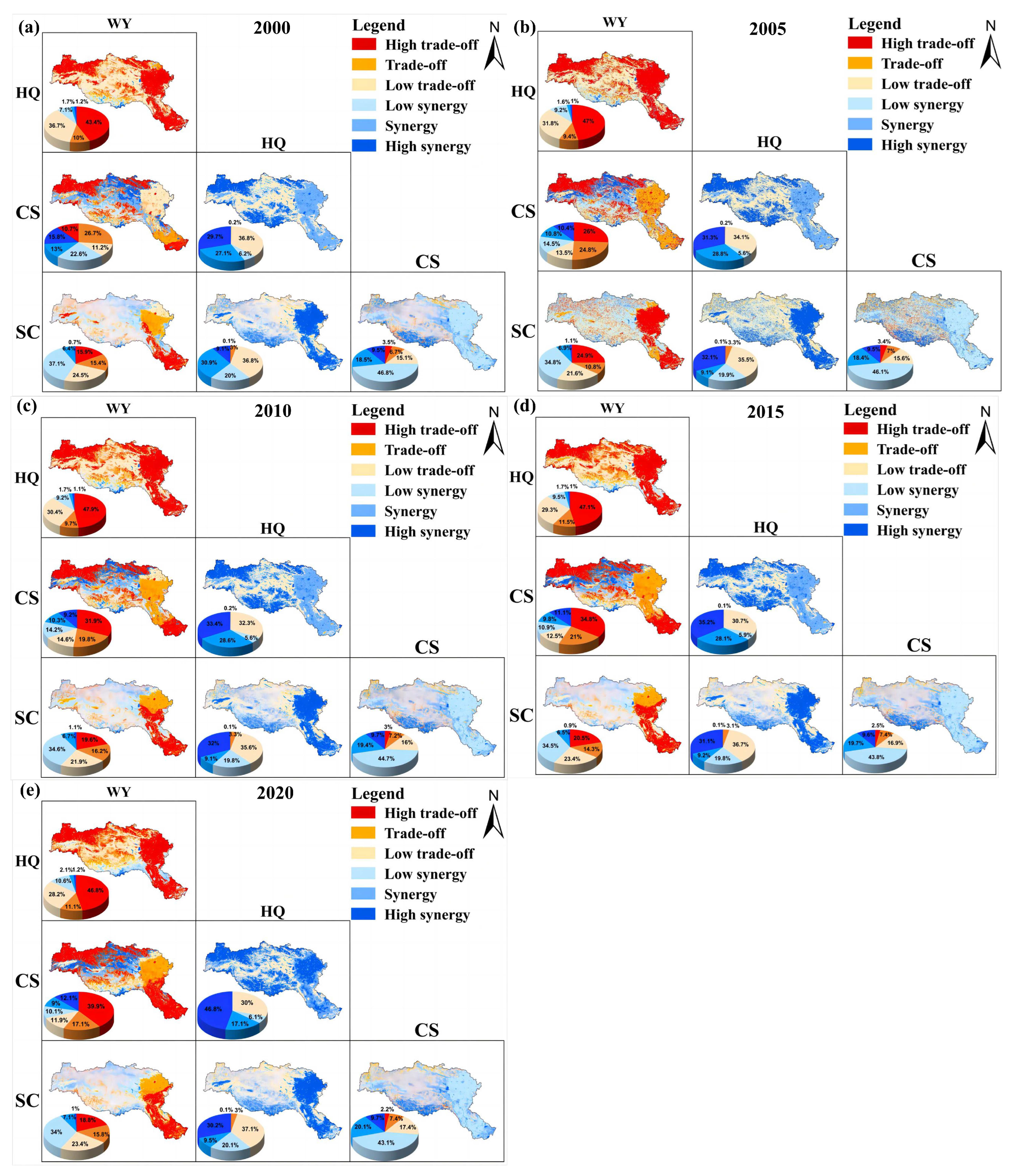
Figure 8 illustrates the spatial trade-off and synergy relationships among four distinct ESs. Generally, a trade-off between WY and CS was observed in the northern and southeastern regions of the HRB. Specifically, the proportion of high-synergy areas increased from 10.7% to 39.9%, while the proportion of synergy areas decreased from 26.7% to 17.1%; the proportion of low-synergy areas decreased from 22.6% to 10.1%. The observed changes were primarily in the middle and lower reaches of the HRB. A predominance of regions with low trade-offs and low synergy was exhibited by WY and SC, accounting for 57.4% of the study area. Moreover, a shift from low-trade-off to high-trade-off areas was observed in the cities of Hanzhong, Zaoyang, and the Tongbai Mountain area. The proportion of regions with high trade-offs between WY and SC increased from 15.9% to 18.8%, while the proportion of regions with low synergy between WY and SC decreased from 37.1% to 34%. For HQ and CS, there was a trend of low trade-off in most main stream and tributary areas. Meanwhile, an increase in the proportion of synergy areas was observed from 2001 to 2020, rising from 63.2% to 70%. In particular, the transition from low synergy to high synergy was observed in the eastern agricultural areas, while the transition from low trade-off to low synergy occurred in the northern Qinling Mountains. The relationship between HQ and SC was characterized by a synergy trend in more than 60% of the study area. A trade-off trend was mainly observed in the northern areas of Danjiangkou and around Hanzhong-Ankang City. Few changes were observed in the trade-off and synergy between HQ and SC during the research period, while a shift from low synergy, synergy, and low trade-off to high synergy occurred in the Dabie Mountain region and Wuhan city. The proportion of high-synergy areas increased from 9.1% to 30.2%, while the proportion of low-synergy areas decreased from 30.9% to 9.5%. The main manifestation between SC and CS was a synergy trend (73% of the study area), with a small portion being characterized by a trade-off trend, primarily distributed in the area surrounding the northern Qinling Mountains, Daba Mountains, and Dahong Mountains. Similarly, relatively small changes in the trade-off/synergy relationship between SC and CS were observed from 2001 to 2020, with the most obvious change located in the northern Qinling Mountains.

3.4. Spatial-Temporal Patterns of ESBs

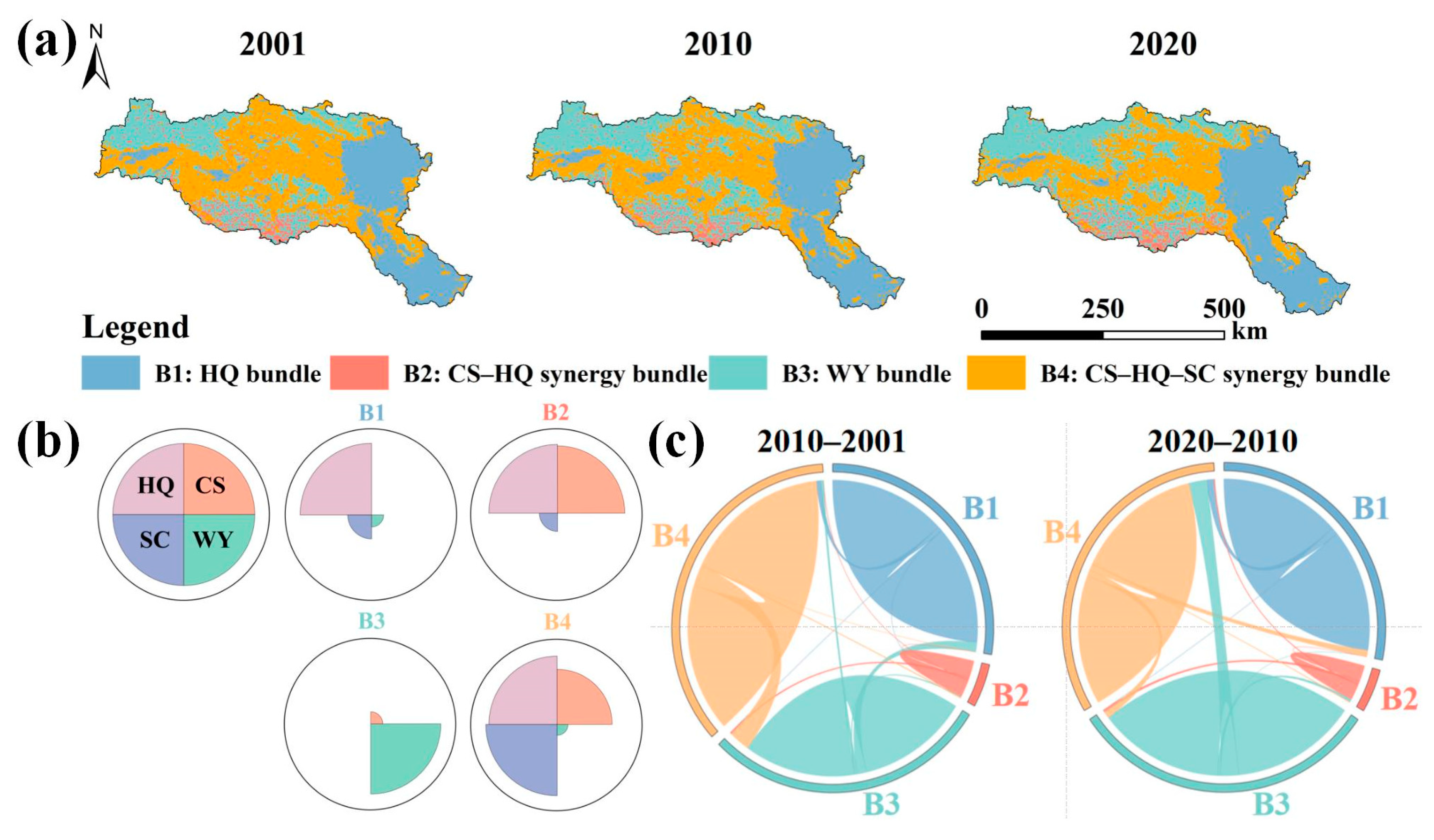
Initially, the Self-Organizing Map (SOM) identified four ES bundles at the grid scale. Subsequently, the study area was divided into these four bundles, considering the synergistic and trade-off effects of the ESs in the HRB (Figure 9a). The transition characteristics of the four ES bundles, identified by the SOM at the grid scale, were also analyzed (Figure 9b). Bundle 1 was primarily distributed around Nanyang City and the Jingmen-Wuhan urban area, accounting for 28.21%, 29.18%, and 29.46% of the study area in 2001, 2010, and 2020, with cropland being the predominant land use type, which exhibited a higher level of HQ but lower levels of SC and WY. During the study period, the area of bundle 1 demonstrated an increasing trend, which was mainly observed in the surrounding areas of Xiangyang City and Jingmen City, with only a decreasing trend occurring in the Hanyin-Ankang area. Bundle 2 was mainly distributed around the Daba Mountains and the northwest region of Hanzhong City, accounting for 4.82%, 4.79%, and 4.74% of the study area in 2001, 2010, and 2020, with grassland being the dominant land use type, which had higher levels of HQ and CS but low levels of SC and WY. The area of bundle 2 was relatively stable throughout the study period, with the increase primarily attributed to the transformation of bundle 4 in the western Daba Mountains area. Bundle 3 was mainly distributed in the Qinling Mountains, Waifang Mountains, and Funiu Mountains, accounting for 40.44%, 30.92%, and 33.77% of the study area in 2001, 2010, and 2020, characterized by forestland use with a high WY. Overall, bundle 3 displayed a growth trend during the study period. The growth of bundle 3 primarily originated from the transformation of bundle 4 from 2001 to 2010, while bundle 3 exhibited a weak decreasing trend from 2010 to 2020. Bundle 4 was mainly distributed in the upstream region of the HRB, accounting for 26.52%, 35.10%, and 32.03% of the study area in 2001, 2010, and 2020, with grassland and wetland being the predominant land use types, and had higher levels of SC and HQ but weaker levels of CS compared to bundle 2. The area of bundle 4 significantly decreased during the study period, mainly due to the transformation of bundle 4 into bundle 3 around the Danjiangkou Reservoir. With the accelerated agricultural specialization and urbanization processes in Xiangyang, Jingmen, and Wuhan City, bundle 4 was gradually replaced by bundles 1 and 3 in the surrounding regions of the city.

3.5. Analysis of Driving Factors of ESs

3.5.1. Factor Impact Detection Analysis

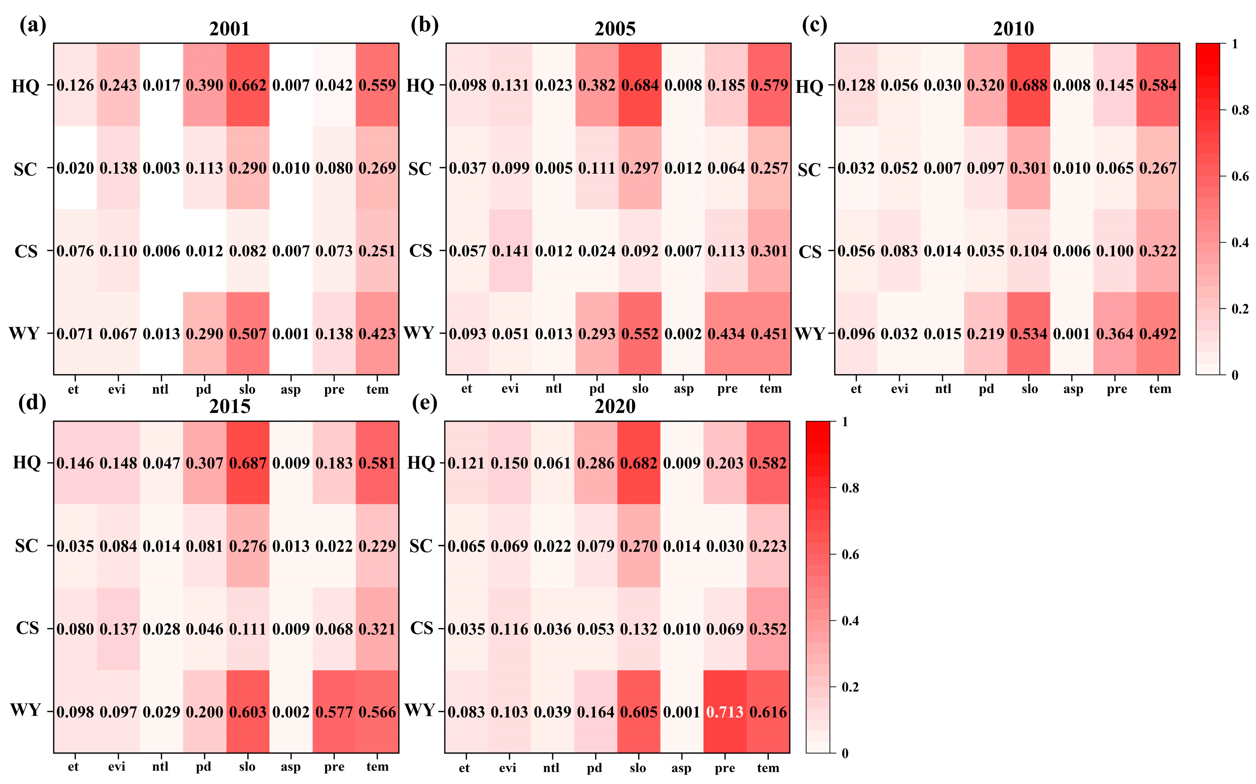
The factor detector was employed to analyze the impact of various factors on the spatial distribution of ESs in 2001, 2005, 2010, 2015, and 2020 (Figure 10). The findings indicated that key factors in each year include population density, slope, precipitation, and temperature. In 2001, slope (q > 0.5) emerged as the primary driving factor for changes in the spatial distribution of ESs, particularly influencing WY. Population density and temperature also showed obvious effects with q > 0.2. Temperature (q > 0.25) had the most significant impact on CS. For SC, slope assumed the role of the dominant factor (q > 0.29), while temperature (q > 0.26) remained an important influencing factor. Regarding HQ, slope (q > 0.66) had the greatest impact, with population density and slope also demonstrating crucial influences (q > 0.35). Although the most influential factors for each ES remained relatively constant from 2005 to 2015, their respective q values increased slightly. In 2020, precipitation emerged as the paramount influencing factor for WY, with a q value of 0.71. The influence of the night light index and slope direction on the spatial distribution of ESs was negligible (q < 0.02) during the selected years. Overall, the ranking of factors was established according to the q values as follows: slope > temperature > precipitation > population density > enhanced vegetation index > evapotranspiration > night light index > slope direction. The impact of temperature, precipitation, and population density remained relatively stable over time. The spatial distribution of vegetation from 2001 to 2020 was influenced by various environmental factors, with natural factors having a more pronounced influence than human factors.

3.5.2. Factor Interaction Detection Analysis

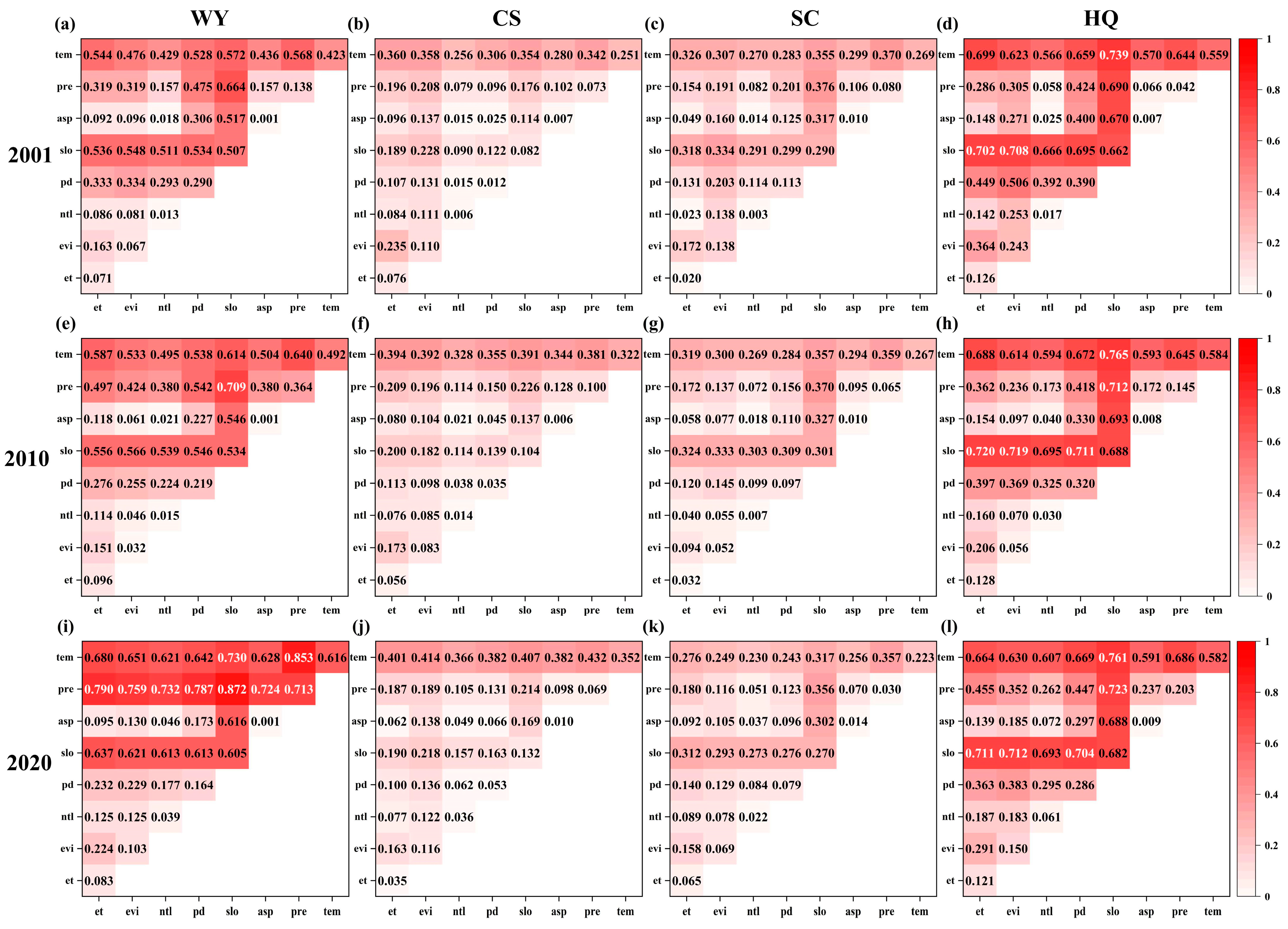
Figure 11 illustrates the impact of the interaction between two factors on the spatial distribution of ESs. The results showed that the combined impact of two factors on the spatial distribution of ESs was greater than that of any single factor. Among the three selected representative years (2001, 2010, and 2020), within the combination of these two factors affecting WY, the q-values of those two factors were higher than those of individual factors. The combined influence of terrain factors and natural factors held more substantial sway over the spatial distribution of ESs in comparison to individual factors. The highest q-value for the interaction indicated the significance of the interaction between slope, temperature, precipitation, and population density in shaping the spatial variation of ESs. Furthermore, the most considerable q-value for the interaction in 2019 pertained to slope and temperature. This indicated that the interaction between terrain factors significantly contributed to explaining ESs, further validating the dominant role of terrain factors.

4. Discussion

4.1. Spatiotemporal Dynamics and Driving Factors of ESs

This study revealed that the value of WY exhibited a continuous decreasing trend before 2015 and an increase thereafter in the HRB, aligning with the findings of Qi, Li, Zhang and Zhang [8]. These changes were attributable to the transformation of grasslands and croplands into forests (Figure 2) because forests had higher evapotranspiration compared to other vegetation types [8]. Prior research indicated that extensive afforestation in shrubland areas can markedly decrease regional runoff, potentially leading to reduced regional WY. [38]. In addition, previous studies have confirmed a close correlation between WY and precipitation within the watershed [5]. The study area was characterized by low precipitation in the north and high precipitation in the south, and as a result of the influence of the Qinling mountains in the north, the annual precipitation remained stable at around 700 mm, which led to an insignificant change in WY [39]. In the watershed’s southern and eastern regions, high precipitation led to lower evapotranspiration, resulting in a higher WY in these areas [5]. For CS, the higher CS was mostly observed in the western mountainous areas with significantly increased forest coverage (Figure 2 and Figure 3). Meanwhile, we found that the high CS values mostly occurred in the forest areas, whereas grasslands and bare land dominated low CS values. A consistent conclusion can be seen in the research of Wang and Dai [5], who concluded that forests had a higher CS compared to other vegetation types. Meanwhile, Li, Jiang, Gao and Du [7] also found that in the Northeast Qinghai-Tibet Plateau, the CS decreased from east to northwest, a change attributed to the transition of land types from forests to grasslands. The reason was that the forest had huge canopies and root systems, and forest species diversity can also enhance ecosystem diversity, leading to enhanced carbon storage [5]. Overall, this study concluded that the proportion of forestland CS increased from 51.4% to 59.48%, and the total CS in grassland decreased from 24.46% to 18.4%, which can be attributed to the extensive conversion of grasslands and cropland to forests in the central and western regions of the HRB (Figure 2). For HQ, areas of higher quality were predominantly located upstream in the watershed, specifically in regions with dense forest coverage like the southern Qinling and northern Daba mountains. In contrast, lower values were observed primarily in the grassland-covered hilly regions downstream. (Figure 2 and Figure 3). The reason was that compared to forest ecosystems, grassland ecosystems were more fragile, with poorer resistance and stability and lower biodiversity [40], therefore resulting in a low HQ. From 2001 to 2020, due to the increase in urban construction land in most areas of Shaanxi Province upstream of the watershed and Hubei Province downstream of the watershed [9], the HQ in the vicinity of these towns decreased [21]. However, the HQ had obviously improved due to good ecological protection and an increase in grassland and forest area around most cities downstream of the watershed [22]. Overall, the distribution and changes in HQ were closely related to land-use types and vegetation coverage [41]. This study revealed that regions with high total SC predominantly occur in the mountainous upper regions of the study area, particularly in the southern Qinling and northern Daba mountains. (Figure 3). Although the upper reaches of the HRB had relatively abundant precipitation, more complex terrain, and strong potential soil erosion, due to the high forest coverage in these areas [42], plant roots can play an obvious consolidation role in the soil [43]. In addition, the vertical structure of vegetation patterns was relatively complete, which can not only reduce soil erosion by precipitation but also regulate runoff, thereby reducing the actual amount of soil erosion, resulting in a large amount of SC in these areas [24,26]. However, the vegetation types in the downstream areas of the watershed were relatively single and there were many cultivated lands, resulting in severe soil erosion [44]. In addition, we found that the SC downstream of the watershed gradually increased from 2001 to 2020, especially in the southern part of Funiu mountains, the western part of Tongbai County, and the surrounding area of Tianmen River (Figure 3). These changes were primarily attributed to the implementation of the policy that reverts farmland to forests and grasslands, along with changes in land-use methods [42,45]. In this study, we found that slope and temperature are the two dominant factors. According to the research results, the areas with high slopes and fewer human activities have higher carbon storage. In the role of topography and geomorphology in regional soil conservation, slope was also a key factor. The larger the slope was, the more easily it caused soil and water movement, forming accumulation and loss, while a smaller slope can inhibit water production in the basin to a certain extent and play the role of soil and water conservation [46]. Temperature was negatively correlated with ESs, which was consistent with the research results of [47]. Temperature affects water yield and its coverage to a certain extent, and then affects ESs. Meanwhile, a previous study had concluded that the temperature will decrease with the increase in slope, indicating that the heat on the slope will decrease with the increase in slope; that is, the slower the slope, the more heat received per unit area because different slopes affect the angle of the sun’s light incident on the surface, which in turn affects the surface to receive solar radiation energy [48].

4.2. The Trade-Offs/Synergies among Multiple ESs

Environmental factor changes will continually alter the trade-offs and synergies among various ecological services, leading to clear spatial heterogeneity in the interactions between these services [4,7,49]. For example, an increase in precipitation will supplement regional water sources and increase soil erosion to a certain extent, thereby increasing regional WY and SC, resulting in a synergistic relationship between the two ESs [7]. However, if precipitation intensity and surface runoff surpass vegetation’s erosion resistance, this could lead to increased soil erosion. Consequently, the soil conservation ability of vegetation may diminish, ultimately influencing the balance between WY and SC [50]. In addition, an increase in temperature will promote the improvement of photosynthesis, leading to an increase in carbon storage [51]. However, when the temperature exceeds the optimal temperature for photosynthesis, it will inhibit the CS function of vegetation [52]. Consequently, temperature fluctuations will modify the balance and synergy between CS and other ESs. Additionally, the transformation of land-use types significantly impacted the balance and cooperative interactions among different ESs. For instance, forests exhibited more robust SC and CS than grasslands [53].
In this study, we conducted a spatial evaluation of the trade-off/synergistic relationship between multiple ESs in the HRB from 2001 to 2020 and found that the trade-off relationship between WY and the other three ESs played a dominant role, while the synergistic relationship accounted for relatively little (Figure 8), especially in the northwest and southeast regions of the study area. Previous research has shown that an increase in soil conservation may cause an increase in soil thickness, which in turn hinders rainfall infiltration into the soil [54]. Vegetation can obtain less soil moisture, ultimately leading to a decrease in WY. The decrease in WY weakened the erosion effect of runoff on surface soil, thus increasing soil conservation [55]. Additionally, transforming other land types into forests in these regions had resulted in increased regional water consumption, as the increase in forest area enhanced the overall transpiration of vegetation, coupled with fluctuations in rainfall, ultimately leading to a decrease in WY [8,53]. Meanwhile, we found that the synergistic relationship between HQ, CS, and SC dominated, mainly occurring in the northern and eastern regions of the study area. From 2001 to 2020, these regions underwent significant land-use changes as a substantial portion of arable land and grassland was transformed into forests (Figure 2). The increase in forest area indicated an increase in vegetation coverage, which can significantly reduce the erosion of rainwater on the ground and reduce soil erosion [56,57]. Forests had deeper root systems in the soil layer, and root biomass density can significantly affect soil conservation services, thereby increasing SC [55]. This aligns with Wang, et al. [58]’s findings that in the Loess Plateau region, soil erosion resistance increased with higher root zone density and more soil organic matter. Meanwhile, compared to grasslands and arable land, the increase in forest area can further enhance carbon storage and carbon sink potential [3,53]. Wang, Zhao, Xu, Ding, Yan and Sofia Santos Ferreira [53] revealed differences in ecosystem services between artificial forests and natural grasslands by examining functional traits. It found that in the loess hilly area, artificial forests provided stronger soil conservation and carbon storage services than natural grasslands. Therefore, land-use change, especially the increase in forests, can not only improve SC but also significantly increase carbon sink [3], thereby presenting a highly synergistic relationship between CS and SC. In addition, this study found a high degree of synergy between HQ, CS, and SC. As shown in Figure 4, from 2001 to 2020, the SC and CS in the study area continued to increase, and the score of HQ continued to improve. The three services showed a synergistic effect of mutual promotion. This was mainly due to the continuous improvement of forestland quality in recent years, which promoted the strengthening of vegetation fix carbon ability [59,60]. Good forest vegetation had a strong interception effect on rainfall, while the lush vegetation canopy reduced the erosion of rainwater on the soil surface to some extent, leading to a gradual shift in the direction of mutual synergy among ecosystem services, and the degree of synergy also increased [53,56].

4.3. Implications for Landscape Management

As the water source of the Middle Route of the South-to-North Water Diversion Project, maintaining the stability and improvement of ESs in the HRB was of great strategic significance for the whole country [61]. By analyzing the spatiotemporal variation and ESBs, the following scientific and reasonable reference measures can be provided for future ecosystem management in the HRB. Specifically, bundle 1 was mainly covered by cropland land, and these areas had higher HQ but lower WY and SC (Figure 9a). Therefore, these regions should consider the protection of arable land, limit the area of construction land, and prevent the blind expansion and disorderly spread of cities and towns [62]. Meanwhile, in steep-slope cultivated areas, planting trees and grass should be strengthened, which can not only aid in food security but also further improve WY and SC [8,63]. Although the main cover type of bundle 2 was grassland and it had high CS and HQ, WY and SC were still relatively low (Figure 9a). Therefore, these regions should continue ecological protection to maintain the stability of CS and HQ, and should be banned or replanted with soil and water conservation forests to enhance soil and water conservation capacity and improve WY [18]. Bundle 3 was mainly distributed in mountain areas such as the Qinling Mountains, Waifang Mountains, and Funiu Mountains, where the vegetation type was mainly forest and had a high WY (Figure 9a,b). However, these areas were also important areas for mineral resource enrichment, with a high level of mining and development. Therefore, for the mountainous areas in the northern part of the watershed, it was necessary to strengthen the ecological restoration of mining and comprehensive management of mining subsidence areas and improve the self-restoration ability of the ecological system [64], which can not only maintain high WY but also strengthen soil and water conservation and CS in these areas. The main cover types of bundle 4 were grassland and wetland, which had high ecological service capabilities and belonged to a highly synergistic relationship of CS, HQ, and SC. Future land management should ensure the coexistence of land-use development and carbon emission reduction [34]. It was necessary to protect carbon sink land, improve the quality of wetlands around the Danjiangkou reservoir, and promote the construction of green mines [65]. Meanwhile, efforts should also be made to increase ecological restoration, further providing CS and SC for the region, and thereby improving the regional HQ [3,45]. Overall, to achieve the carbon neutrality goal and optimize the land-use structure of the HRB in the future, it was essential to comprehensively consider cropland protection, controlling the expansion of construction land in low-altitude areas in the east and southeast [66,67]. For areas with low soil and water conservation, vegetation restoration should be strengthened [11,45], especially through afforestation to increase regional WY and provide more sufficient water sources for the South-to-North Water Diversion Project.

4.4. Limitations and Next Steps

This study’s evaluation results revealed the spatiotemporal variation characteristics of ESs in the HRB, although uncertainties persisted in the findings. Firstly, although the InVEST model was relatively mature, it still had certain limitations, such as the WY module being unable to effectively consider the impact of terrain [5]. Secondly, the input data of the model will also affect the research results; the root depth, pawc, sensitivity of threat, and other parameters were also determined based on empirical data in the model user manual and relevant literature; human data such as population density were obtained through spatial assignment, and the accuracy was highly affected by resolution. In addition, land-use data were crucial for evaluating ESs, and the accuracy of land-use products based on remote sensing interpretation (MCD12Q1) also needed further verification [45]. Although this study can identify the spatial locations where the trade-off relationships between multiple ESs occur through the trade-off and collaborative analysis of ESs in the HRB, which helped to balance management decisions with specific spatial locations, it only analyzed the ESs of a specific year, reflecting the changing trends between different time nodes, which does not allow us to determine the variability of ESs over time in a long time series [7]. Moreover, due to the limitations of large-scale field observations, this study did not use field-measured data to verify the simulation results of different ESs. Therefore, future research will attempt to validate the simulation results of different ecological service functions through large-scale field investigations and observations. Therefore, future research should fully consider the following aspects: (1) selecting land-use data with higher precision and finer division as much as possible; (2) obtaining climate, soil, and human data of the study area through field research; (3) further integrating and comprehensively considering the impact of various factors such as the environment, human activities, differences in vegetation types, and vegetation age structure on the ESs; (4) considering using other land-use simulation models to simulate the land cover in the study area, such as the FLUS model; (5) using long-term time-series data for long-term spatiotemporal-scale monitoring and evaluation of ESs to reveal the evolution trend and local characteristics of ES relationships; and (6) attempting to validate the simulation results of different ESs through large-scale field investigations and observations.

5. Conclusions

In this study, we analyzed the spatiotemporal changes in ESs, hot spots, and ESBs during 2001–2020 in the HRB. Meanwhile, the trade-offs and synergistic relationships between ESs and the socioecological driving factors of these ESs were examined. During 2001–2020, the forests, wetlands, urban construction land, and water bodies increased by 11732.1 km2, 485.85 km2, 407.2 km2, and 162.36 km2 in the HRB, respectively. Temporally, except for SC showing a trend of first increasing and then stabilizing, WY, CS, and SC all showed a continuously increasing trend. Spatially, WY and HQ exhibited bipolar clustering characteristics, with WY exhibiting low-value clustering in the upstream and high-value clustering in the downstream, while the pattern of HQ was the opposite; CS exhibited differentiated clustering characteristics, with high- and low-value areas distributed throughout the entire watershed. In CS and HQ, the spatial patterns of cold and hot spots were quite similar: hot spots were primarily in the basin’s western and central areas, while cold spots were mostly in the eastern and southeastern regions. Correlation analysis revealed a significant positive correlation between HQ and CS, a significant negative correlation between WY and CS, and only a weak correlation among other service functions. Spatially, WY, HQ, CS, and SC showed a high trade-off relationship in most areas, especially in the northwest and southeast parts of the study area. However, HQ, CS, and SC mainly exhibited a synergistic relationship, and most regions showed mild synergy between CS and SC. The slope and temperature have high influencing factor coefficients on various ESs. The combined influence of terrain and natural factors had a more significant impact on the spatial distribution of ESs than any single factor, with terrain factors playing a dominant role in explaining the changes in these ESs.

Author Contributions

P.H.: conceptualization, methodology, software, formal analysis, writing—original draft. G.Y.: conceptualization, modifying figures. Z.W. (Zijun Wang): data curation, software, formal analysis. Y.L.: conceptualization, methodology, project administration, funding acquisition, supervision. X.C.: data curation, formal analysis. W.Z.: methodology, conceptualization. Z.Z.: Data curation. Z.W. (Zhongming Wen): methodology, project administration, conceptualization. H.S.: data curation. Z.L.: methodology, software. H.R.: data curation. All authors have read and agreed to the published version of the manuscript.

Funding

This research was funded by the Special project of science and technology innovation plan of Shaanxi Academy of Forestry Sciences (No. SXLK2022–02-7 and No. SXLK2023–02-14), the National Natural Science Foundation of China (No. 42107512), the Key R&D Plan of Shaanxi Province (No. 2024SF-YBXM-621), the Open Research Fund of State Key Laboratory of Simulation and Regulation of Water Cycle in River Basin, China Institute of Water Resources and Hydropower Research, Grant NO. IWHR-SKL-KF202315, and the Open Research Fund of Key Laboratory of Digital Earth Science, Chinese Academy of Sciences (No. 2022LDE003).

Data Availability Statement

Data is contained within the article.

Acknowledgments

We also acknowledge the data support from “Loess plateau science data center, National Earth System Science Data Sharing Infrastructure, National Science & Technology Infrastructure of China (http://loess.geodata.cn, accessed on 1 October 2023)”. There is no new data were created in this research.

Conflicts of Interest

The authors declare that they have no known competing financial interests or personal relationships that could have appeared to influence the work reported in this paper.

References

  1. MEA. Ecosystems and Human Well-Being: Synthesis; Millennium Ecosystem Assessment; Island Press: Washington, DC, USA, 2005. [Google Scholar]
  2. Li, Y.; Luo, H. Trade-off/synergistic changes in ecosystem services and geographical detection of its driving factors in typical karst areas in southern China. Ecol. Indic. 2023, 154, 110811. [Google Scholar] [CrossRef]
  3. Liu, X.; Ding, J.; Zhao, W. Divergent responses of ecosystem services to afforestation and grassland restoration in the Tibetan Plateau. J. Environ. Manag. 2023, 344, 118471. [Google Scholar] [CrossRef] [PubMed]
  4. Geng, W.; Li, Y.; Zhang, P.; Yang, D.; Jing, W.; Rong, T. Analyzing spatio-temporal changes and trade-offs/synergies among ecosystem services in the Yellow River Basin, China. Ecol. Indic. 2022, 138, 108825. [Google Scholar] [CrossRef]
  5. Wang, Y.; Dai, E. Spatial-temporal changes in ecosystem services and the trade-off relationship in mountain regions: A case study of Hengduan Mountain region in Southwest China. J. Clean. Prod. 2020, 264, 121573. [Google Scholar] [CrossRef]
  6. Su, B.; Liu, M. An ecosystem service trade-off management framework based on key ecosystem services. Ecol. Indic. 2023, 154, 110894. [Google Scholar] [CrossRef]
  7. Li, G.; Jiang, C.; Gao, Y.; Du, J. Natural driving mechanism and trade-off and synergy analysis of the spatiotemporal dynamics of multiple typical ecosystem services in Northeast Qinghai-Tibet Plateau. J. Clean. Prod. 2022, 374, 134075. [Google Scholar] [CrossRef]
  8. Qi, W.; Li, H.; Zhang, Q.; Zhang, K. Forest restoration efforts drive changes in land-use/land-cover and water-related ecosystem services in China’s Han River Basin. Ecol. Eng. 2019, 126, 64–73. [Google Scholar] [CrossRef]
  9. Zheng, L.; Wang, Y.; Li, J. Quantifying the spatial impact of landscape fragmentation on habitat quality: A multi-temporal dimensional comparison between the Yangtze River Economic Belt and Yellow River Basin of China. Land Use Policy 2023, 125, 106463. [Google Scholar] [CrossRef]
  10. Vačkářová, D.; Medková, H.; Krpec, P.; Weinzettel, J. Ecosystem services footprint of international trade: Economic value of ecosystem services lost due to crop production. Ecosyst. Serv. 2023, 64, 101560. [Google Scholar] [CrossRef]
  11. Li, J.; Dong, S.; Li, Y.; Wang, Y.; Li, Z. Terrestrial transect study on pattern and driving mechanism of ecosystem services in the China–Mongolia–Russia Economic Corridor. Sci. Total Environ. 2023, 884, 163880. [Google Scholar] [CrossRef]
  12. Yu, F.; Li, C.; Yuan, Z.; Luo, Y.; Yin, Q.; Wang, Q.; Hao, Z. How do mountain ecosystem services respond to changes in vegetation and climate? An evidence from the Qinling Mountains, China. Ecol. Indic. 2023, 154, 110922. [Google Scholar] [CrossRef]
  13. Zhang, J.; Guo, W.; Cheng, C.; Tang, Z.; Qi, L. Trade-offs and driving factors of multiple ecosystem services and bundles under spatiotemporal changes in the Danjiangkou Basin, China. Ecol. Indic. 2022, 144, 109550. [Google Scholar] [CrossRef]
  14. Ran, P.; Hu, S.; Frazier, A.E.; Yang, S.; Song, X.; Qu, S. The dynamic relationships between landscape structure and ecosystem services: An empirical analysis from the Wuhan metropolitan area, China. J. Environ. Manag. 2023, 325, 116575. [Google Scholar] [CrossRef]
  15. Wu, K.; Wang, D.; Lu, H.; Liu, G. Temporal and spatial heterogeneity of land use, urbanization, and ecosystem service value in China: A national-scale analysis. J. Clean. Prod. 2023, 418, 137911. [Google Scholar] [CrossRef]
  16. Xue, C.; Chen, X.; Xue, L.; Zhang, H.; Chen, J.; Li, D. Modeling the spatially heterogeneous relationships between tradeoffs and synergies among ecosystem services and potential drivers considering geographic scale in Bairin Left Banner, China. Sci. Total Environ. 2023, 855, 158834. [Google Scholar] [CrossRef]
  17. Zhu, C.; Zhang, X.; Zhou, M.; He, S.; Gan, M.; Yang, L.; Wang, K. Impacts of urbanization and landscape pattern on habitat quality using OLS and GWR models in Hangzhou, China. Ecol. Indic. 2020, 117, 106654. [Google Scholar] [CrossRef]
  18. Liu, Z.; Huang, Q.; Zhou, Y.; Sun, X. Spatial identification of restored priority areas based on ecosystem service bundles and urbanization effects in a megalopolis area. J. Environ. Manag. 2022, 308, 114627. [Google Scholar] [CrossRef]
  19. Wu, L.; Sun, C.; Fan, F. Multi-criteria framework for identifying the trade-offs and synergies relationship of ecosystem services based on ecosystem services bundles. Ecol. Indic. 2022, 144, 109453. [Google Scholar] [CrossRef]
  20. Xia, H.; Yuan, S.; Prishchepov, A.V. Spatial-temporal heterogeneity of ecosystem service interactions and their social-ecological drivers: Implications for spatial planning and management. Resour. Conserv. Recycl. 2023, 189, 106767. [Google Scholar] [CrossRef]
  21. Tu, D.; Cai, Y.; Liu, M. Coupling coordination analysis and spatiotemporal heterogeneity between ecosystem services and new-type urbanization: A case study of the Yangtze River Economic Belt in China. Ecol. Indic. 2023, 154, 110535. [Google Scholar] [CrossRef]
  22. Chen, S.; Wen, Z.; Zhang, S.; Huang, P.; Ma, M.; Zhou, X.; Liao, T.; Wu, S. Effects of long-term and large-scale ecology projects on forest dynamics in Yangtze River Basin, China. For. Ecol. Manag. 2021, 496, 119463. [Google Scholar] [CrossRef]
  23. Peng, Y.; Chen, W.; Pan, S.; Gu, T.; Zeng, J. Identifying the driving forces of global ecosystem services balance, 2000–2020. J. Clean. Prod. 2023, 426, 139019. [Google Scholar] [CrossRef]
  24. Xie, T.; Zhang, G.; Hou, J.; Xie, J.; Lv, M.; Liu, F. Hybrid forecasting model for non-stationary daily runoff series: A case study in the Han River Basin, China. J. Hydrol. 2019, 577, 123915. [Google Scholar] [CrossRef]
  25. Liu, Y.; Jing, Y.; Han, S. Multi-scenario simulation of land use/land cover change and water yield evaluation coupled with the GMOP-PLUS-InVEST model: A case study of the Nansi Lake Basin in China. Ecol. Indic. 2023, 155, 110926. [Google Scholar] [CrossRef]
  26. Fu, W.; Cao, Y.; Li, X.; Sun, J.; Liu, F.; Li, W. The responses of riparian plant communities to environmental and spatial factors in the upper Han River Basin, China. Glob. Ecol. Conserv. 2022, 36, e02118. [Google Scholar] [CrossRef]
  27. Bai, X.; Zhao, W. Impacts of climate change and anthropogenic stressors on runoff variations in major river basins in China since 1950. Sci. Total Environ. 2023, 898, 165349. [Google Scholar] [CrossRef]
  28. Hou, W.; Hu, T.; Yang, L.; Liu, X.; Zheng, X.; Pan, H.; Zhang, X.; Xiao, S.; Deng, S. Matching ecosystem services supply and demand in China’s urban agglomerations for multiple-scale management. J. Clean. Prod. 2023, 420, 138351. [Google Scholar] [CrossRef]
  29. Hamel, P.; Bryant, B.P. Uncertainty assessment in ecosystem services analyses: Seven challenges and practical responses. Ecosyst. Serv. 2017, 24, 1–15. [Google Scholar] [CrossRef]
  30. Lal, R. Soil Carbon Sequestration Impacts on Global Climate Change and Food Security. Science 2004, 304, 1623–1627. [Google Scholar] [CrossRef] [PubMed]
  31. Nelson, E.; Polasky, S.; Lewis, D.J.; Plantinga, A.J.; Lonsdorf, E.; White, D.; Bael, D.; Lawler, J.J. Efficiency of incentives to jointly increase carbon sequestration and species conservation on a landscape. Proc. Natl. Acad. Sci. USA 2008, 105, 9471–9476. [Google Scholar] [CrossRef] [PubMed]
  32. Renard, K.G.; Freimund, J.R. Using monthly precipitation data to estimate the R-factor in the revised USLE. J. Hydrol. 1994, 157, 287–306. [Google Scholar] [CrossRef]
  33. Wischmeier, W.H.; Smith, D.D. Predicting Rainfall Erosion Losses: A guide to Conservation Planning; Agriculture Handbook No. 537; U.S. Department of Agriculture: Washington, DC, USA, 1978. [Google Scholar]
  34. Wang, Y.; Liu, Y.; Wang, Z.; Zhang, Y.; Fang, B.; Jiang, S.; Yang, Y.; Wen, Z.; Zhang, W.; Zhang, Z.; et al. Assessing the Spatio-Temporal Dynamics of Land Use Carbon Emissions and Multiple Driving Factors in the Guanzhong Area of Shaanxi Province. Sustainability 2023, 15, 7730. [Google Scholar] [CrossRef]
  35. Anselin, L. Local indicator of Spatial Association-LISA. Geogr. Anal. 1998, 27, 93–115. [Google Scholar] [CrossRef]
  36. Raudsepp-Hearne, C.; Peterson, G.D.; Bennett, E.M. Ecosystem service bundles for analyzing tradeoffs in diverse landscapes. Proc. Natl. Acad. Sci. USA 2010, 107, 5242–5247. [Google Scholar] [CrossRef] [PubMed]
  37. Bennett, E.M.; Peterson, G.D.; Gordon, L.J. Understanding relationships among multiple ecosystem services. Ecol. Lett. 2009, 12, 1394–1404. [Google Scholar] [CrossRef] [PubMed]
  38. Farley, K.A.; Jobbágy, E.G.; Jackson, R.B. Effects of afforestation on water yield: A global synthesis with implications for policy. Glob. Chang. Biol. 2005, 11, 1565–1576. [Google Scholar] [CrossRef]
  39. Xie, G.; Chu, K. Determination of corporate water consumption: Evidence from precipitation risks in China. Sci. Total Environ. 2023, 894, 164979. [Google Scholar] [CrossRef]
  40. Shi, Z.; Zhou, S. A study on the dynamic evaluation of ecosystem health in the Yangtze river Basin of China. Ecol. Indic. 2023, 153, 110445. [Google Scholar] [CrossRef]
  41. Fang, L.; Wang, L.; Chen, W.; Sun, J.; Cao, Q.; Wang, S.; Wang, L. Identifying the impacts of natural and human factors on ecosystem service in the Yangtze and Yellow River Basins. J. Clean. Prod. 2021, 314, 127995. [Google Scholar] [CrossRef]
  42. Ren, H.; Wen, Z.; Liu, Y.; Lin, Z.; Han, P.; Shi, H.; Wang, Z.; Su, T. Vegetation response to changes in climate across different climate zones in China. Ecol. Indic. 2023, 155, 110932. [Google Scholar] [CrossRef]
  43. Osawa, T.; Kohyama, K.; Mitsuhashi, H. Trade-off relationship between modern agriculture and biodiversity: Heavy consolidation work has a long-term negative impact on plant species diversity. Land Use Policy 2016, 54, 78–84. [Google Scholar] [CrossRef]
  44. Su, Z.-A.; Zhou, T.; Zhang, X.-B.; Wang, X.-Y.; Wang, J.-J.; Zhou, M.-H.; Zhang, J.-H.; He, Z.-Y.; Zhang, R.-C. A Preliminary Study of the Impacts of Shelter Forest on Soil Erosion in Cultivated Land: Evidence from integrated 137Cs and 210Pbex Measurements. Soil Tillage Res. 2021, 206, 104843. [Google Scholar] [CrossRef]
  45. Liu, Y.; Lin, Z.; Wang, Z.; Chen, X.; Han, P.; Wang, B.; Wang, Z.; Wen, Z.; Shi, H.; Zhang, Z.; et al. Discriminating the impacts of vegetation greening and climate change on the changes in evapotranspiration and transpiration fraction over the Yellow River Basin. Sci. Total Environ. 2023, 904, 166926. [Google Scholar] [CrossRef]
  46. Dou, H.; Li, X.; Li, S.; Dang, D.; Li, X.; Lyu, X.; Li, M.; Liu, S. Mapping ecosystem services bundles for analyzing spatial trade-offs in inner Mongolia, China. J. Clean. Prod. 2020, 256, 120444. [Google Scholar] [CrossRef]
  47. Wang, T.; Gong, Z. Evaluation and analysis of water conservation function of ecosystem in Shaanxi Province in China based on “Grain for Green” Projects. Environ. Sci. Pollut. Res. 2022, 29, 83878–83896. [Google Scholar] [CrossRef]
  48. Šafanda, J. Ground surface temperature as a function of slope angle and slope orientation and its effect on the subsurface temperature field. Tectonophysics 1999, 306, 367–375. [Google Scholar] [CrossRef]
  49. Liu, J.; Pei, X.; Zhu, W.; Jiao, J. Understanding the intricate tradeoffs among ecosystem services in the Beijing-Tianjin-Hebei urban agglomeration across spatiotemporal features. Sci. Total Environ. 2023, 898, 165453. [Google Scholar] [CrossRef] [PubMed]
  50. Wang, N.; Bi, H.; Peng, R.; Zhao, D.; Liu, Z. Disparities in soil and water conservation functions among different forest types and implications for afforestation on the Loess Plateau. Ecol. Indic. 2023, 155, 110935. [Google Scholar] [CrossRef]
  51. Wang, D.; Noguchi, T.; Nozaki, T. Increasing efficiency of carbon dioxide sequestration through high temperature carbonation of cement-based materials. J. Clean. Prod. 2019, 238, 117980. [Google Scholar] [CrossRef]
  52. Yang, B.; Gong, J.; Zhang, Z.; Wang, B.; Zhu, C.; Shi, J.; Liu, M.; Liu, Y.; Li, X. Stabilization of carbon sequestration in a Chinese desert steppe benefits from increased temperatures and from precipitation outside the growing season. Sci. Total Environ. 2019, 691, 263–277. [Google Scholar] [CrossRef]
  53. Wang, J.; Zhao, W.; Xu, Z.; Ding, J.; Yan, Y.; Sofia Santos Ferreira, C. Plant functional traits explain long-term differences in ecosystem services between artificial forests and natural grasslands. J. Environ. Manag. 2023, 345, 118853. [Google Scholar] [CrossRef]
  54. Wei, B.; Li, Z.; Duan, L.; Gu, Z.; Liu, X. Vegetation types and rainfall regimes impact on surface runoff and soil erosion over 10 years in karst hillslopes. CATENA 2023, 232, 107443. [Google Scholar] [CrossRef]
  55. Zi, R.; Zhao, L.; Fang, Q.; Qian, X.; Fang, F.; Fan, C. Path analysis of the effects of hydraulic conditions, soil properties and plant roots on the soil detachment capacity of karst hillslopes. CATENA 2023, 228, 107177. [Google Scholar] [CrossRef]
  56. Qiu, S.; Fang, M.; Yu, Q.; Niu, T.; Liu, H.; Wang, F.; Xu, C.; Ai, M.; Zhang, J. Study of spatialtemporal changes in Chinese forest eco-space and optimization strategies for enhancing carbon sequestration capacity through ecological spatial network theory. Sci. Total Environ. 2023, 859, 160035. [Google Scholar] [CrossRef]
  57. Zhang, B.-J.; Zhang, G.-H.; Yang, H.-Y.; Zhu, P.-Z. Temporal variation in soil erosion resistance of steep slopes restored with different vegetation communities on the Chinese Loess Plateau. CATENA 2019, 182, 104170. [Google Scholar] [CrossRef]
  58. Wang, J.; Zhao, W.; Wang, G.; Yang, S.; Pereira, P. Effects of long-term afforestation and natural grassland recovery on soil properties and quality in Loess Plateau (China). Sci. Total Environ. 2021, 770, 144833. [Google Scholar] [CrossRef]
  59. Blanco, J.A.; Durán, M.; Luquin, J.; San Emeterio, L.; Yeste, A.; Canals, R.M. Soil C/N ratios cause opposing effects in forests compared to grasslands on decomposition rates and stabilization factors in southern European ecosystems. Sci. Total Environ. 2023, 888, 164118. [Google Scholar] [CrossRef] [PubMed]
  60. Li, B.; Gao, G.; Luo, Y.; Xu, M.; Liu, G.; Fu, B. Carbon stock and sequestration of planted and natural forests along climate gradient in water-limited area: A synthesis in the China’s Loess plateau. Agric. For. Meteorol. 2023, 333, 109419. [Google Scholar] [CrossRef]
  61. Su, Q.; Chen, X. Efficiency analysis of metacoupling of water transfer based on the parallel data envelopment analysis model: A case of the South–North Water Transfer Project-Middle Route in China. J. Clean. Prod. 2021, 313, 127952. [Google Scholar] [CrossRef]
  62. Zhang, Y.; Wang, L.; Tang, Z.; Zhang, K.; Wang, T. Spatial effects of urban expansion on air pollution and eco-efficiency: Evidence from multisource remote sensing and statistical data in China. J. Clean. Prod. 2022, 367, 132973. [Google Scholar] [CrossRef]
  63. Li, Z.; Sun, X.; Huang, Z.; Zhang, X.; Wang, Z.; Li, S.; Zheng, W.; Zhai, B. Changes in nutrient balance, environmental effects, and green development after returning farmland to forests: A case study in Ningxia, China. Sci. Total Environ. 2020, 735, 139370. [Google Scholar] [CrossRef] [PubMed]
  64. Nassani, A.A.; Aldakhil, A.M.; Zaman, K. Ecological footprints jeopardy for mineral resource extraction: Efficient use of energy, financial development and insurance services to conserve natural resources. Resour. Policy 2021, 74, 102271. [Google Scholar] [CrossRef]
  65. Bi, Y.; Li, M.; Christie, P.; Du, X.; Tian, L.; Gao, X. Evaluating carbon dynamics in soil aggregates using δ13C following long-term vegetation restoration near a surface mine in a semi-arid region. CATENA 2023, 231, 107281. [Google Scholar] [CrossRef]
  66. Liu, Y.; Zhao, L.; Liu, Y.; Huang, Z.; Shi, J.; Wang, Y.; Ma, Y.; Esteban Lucas-Borja, M.; López-Vicente, M.; Wu, G.-L. Restoration of a hillslope grassland with an ecological grass species (Elymus tangutorum) favors rainfall interception and water infiltration and reduces soil loss on the Qinghai-Tibetan Plateau. CATENA 2022, 219, 106632. [Google Scholar] [CrossRef]
  67. Ren, H.; Liu, Y.; Wen, Z.; Shi, H.; Zhou, R.; Wang, Z.; Kareem, H.A.; Zhang, W. Untangling the effects of climate variation and human interference on grassland dynamics in North China. Land Degrad. Dev. 2023, 35, 467–483. [Google Scholar] [CrossRef]
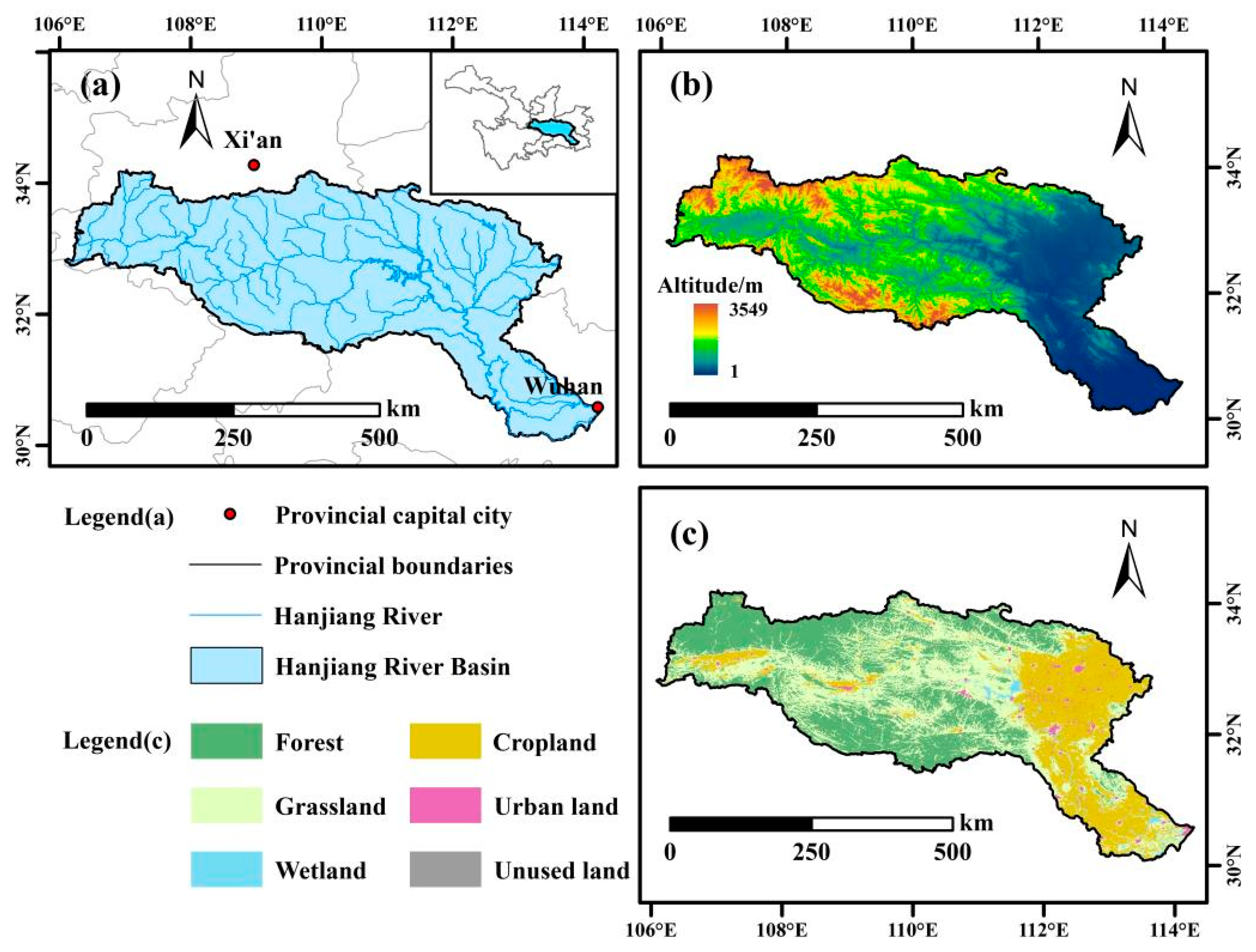
Figure 1. Study area. (a) Location, (b) elevation, and (c) land cover types in the HRB.
Remotesensing 16 02115 g001
Figure 2. The land-use change in HRB from 2001 to 2020. (a) The spatial transformation characteristics of different land uses; (b) the proportion of mutual conversion between different land-use types.
Remotesensing 16 02115 g002
Figure 3. Spatial patterns and changes in ESs in the HRB from 2001–2020. (af) Water yield. (gl) Carbon storage. (mr) Soil conservation. (sx) Habitat quality. (f,l,r,x) Changes in the past 20 years.
Remotesensing 16 02115 g003
Figure 4. Inter-annual variation characteristics of ES values of different land types in the HRB from 2001 to 2020. (a) Carbon storage (b) Water yield (c) Soil conservation (d) Habitat quality values of different land types in the HRB from 2001 to 2020.
Remotesensing 16 02115 g004
Figure 5. Spatial and temporal variation of cold and hot spots of ESs in the HRB from 2001 to 2020. (ae) Water yield. (fj) Carbon storage. (ko) Soil conservation. (pt) Habitat quality.
Remotesensing 16 02115 g005
Figure 6. Correlation relationships of different ESs on an annual basis. (a) Correlations among the four ESs in 2001. (b) Correlations among the four ESs in 2005. (c) Correlations among the four ESs in 2010. (d) Correlations among the four ESs in 2015. (e) Correlations among the four ESs in 2020.
Remotesensing 16 02115 g006
Figure 7. Correlations of different ESs in terms of 5-year-to-5-year changes. (a) Correlations among the four ESs from 2001 to 2005. (b) Correlations among the four ESs from 2005 to 2010. (c) Correlations among the four ESs from 2010 to 2015. (d) Correlations among the four ESs from 2015 to 2020 (e) Correlations among the four ESs from 2001 to 2020.
Remotesensing 16 02115 g007
Figure 8. Spatial synergy and trade-offs of ES pairs and area percentage in 2001, 2005, 2010, 2015, and 2020. (a) 2001. (b) 2005. (c) 2010. (d) 2015. (e) 2020.
Remotesensing 16 02115 g008
Figure 9. (a) Spatial-temporal pattern changes in ES bundles; (b) composition and relative magnitude of ESs in ES bundles; (c) the area of interconversion among different ES bundles during 2001–2020. Note: WY, water yield; CS, carbon storage; SC, soil conservation; HQ, habitat quality.
Remotesensing 16 02115 g009
Figure 10. Explanatory power of driving factors of ESs based on factor detection analysis in 2001, 2005, 2010, 2015, and 2020. (a) 2001. (b) 2005. (c) 2010. (d) 2015. (e) 2020. (Note: WY, water yield; CS, carbon storage; SC, soil conservation; HQ, habitat quality; et, Evapotranspiration; evi, Enhanced Vegetation Index; ntl, Nighttime lighting index; pd, Population Density; slo, Slope; asp, Aspect; pre, Precipitation; tem, Temperature).
Remotesensing 16 02115 g010
Figure 11. Explanatory power of driving factors of ESs based on factor interaction detection analysis in 2001, 2010, and 2020. (ad) Explanatory power of driving factors of 4 ESs based on factor interaction detection analysis in 2001. (eh) Explanatory power of driving factors of 4 ESs based on factor interaction detection analysis in 2010. (il) Explanatory power of driving factors of 4 ESs based on factor interaction detection analysis in 2020. (Note: WY, water yield; CS, carbon storage; SC, soil conservation; HQ, habitat quality; et, Evapotranspiration; evi, Enhanced Vegetation Index; ntl, Nighttime lighting index; pd, Population Density; slo, Slope; asp, Aspect; pre, Precipitation; tem, Temperature).
Remotesensing 16 02115 g011
Table 1. Data source and description.
Data TypeSpatial ResolutionSource
Precipitation500 mLoess Plateau Science Data Center, National Earth System Science Data Sharing Infrastructure, National Science & Technology Infrastructure of China.
(http://loess.geodata.cn, accessed on 21 March 2024)
Land use/land cover500 mEarth Data Search (https://search.earthdata.nasa.gov/search, accessed on 21 March 2024)
Temperature500 mLoess Plateau Science Data Center, National Earth System Science Data Sharing Infrastructure, National Science & Technology Infrastructure of China.
(http://loess.geodata.cn, accessed on 21 March 2024)
Evapotranspiration500 mLoess Plateau Science Data Center, National Earth System Science Data Sharing Infrastructure, National Science & Technology Infrastructure of China.
(http://loess.geodata.cn, accessed on 21 March 2024)
Digital elevation model (DEM)90 mGeospatial Data Cloud
(https://www.gscloud.cn/, accessed on 21 March 2024)
Carbon Pools Harmonized World Soil Database version
Watershed boundary Geographic remote sensing ecological network platform (www.gisrs.cn, accessed on 21 March 2024)
EVI500 mhttps://earthengine.google.com/, accessed on 21 March 2024
Chinese population density1 kmhttps://www.worldometers.info/world-population/, accessed on 21 March 2024
Nighttime lighting index500 mhttps://www.earthdata.nasa.gov/, accessed on 21 March 2024
Table 2. The area characteristics of land-use changes in the HRB. (Unit: km2).
2020Percent2001PercentChangeChange Percent
Grassland54,307.1134.9566,448.4342.77−12,141.30−18.27
Urbanland2734.081.762326.881.50407.2017.50
Unused land11.350.0133.450.02−22.10−66.07
Forest57,279.1636.8845,547.0629.3211,732.1025.76
Wetland940.890.61455.040.29485.85106.77
Water944.140.61781.780.50162.3620.77
Cropland39,149.9725.2039,774.0625.60−624.09−1.57
Table 3. Global spatial autocorrelation of ESs in the HRB from 2001 to 2020.
YearCarbon StorageSoil ConservationWater YieldHabitat Quality
Moran’s IZ ValueGeneral GMoran’s IZ ValueGeneral GMoran’s IZ ValueGeneral GMoran’s IZ ValueGeneral G
20010.569163.391−0.0000750.138581.803−0.0000010.5841885.455−0.0000030.452111.978−0.000223
20050.563185.712−0.0000750.140495.329−0.0000010.6611174.107−0.0000030.284165.436−0.000212
20100.552170.525−0.0000750.142459.956−0.0000010.6611324.447−0.0000030.47498.815−0.000209
20150.482170.991−0.000070.148479.615−0.0000010.6782735.286−0.0000030.382112.375−0.000198
20200.447159.576−0.0000650.148481.331−0.0000010.7631457.987−0.0000030.45893.964−0.000198
Disclaimer/Publisher’s Note: The statements, opinions and data contained in all publications are solely those of the individual author(s) and contributor(s) and not of MDPI and/or the editor(s). MDPI and/or the editor(s) disclaim responsibility for any injury to people or property resulting from any ideas, methods, instructions or products referred to in the content.