Classification of Grapevine Varieties Using UAV Hyperspectral Imaging

Abstract

Classifying grapevine varieties is crucial in precision viticulture, as it allows for accurate estimation of vineyard row growth for different varieties and ensures authenticity in the wine industry. This task can be performed with time-consuming destructive methods, including data collection and analysis in the laboratory. In contrast, unmanned aerial vehicles (UAVs) offer a markedly more efficient and less restrictive method for gathering hyperspectral data, even though they may yield data with higher levels of noise. Therefore, the first task is the processing of these data to correct and downsample large amounts of data. In addition, the hyperspectral signatures of grape varieties are very similar. In this study, we propose the use of a convolutional neural network (CNN) to classify seventeen different varieties of red and white grape cultivars. Instead of classifying individual samples, our approach involves processing samples alongside their surrounding neighborhood for enhanced accuracy. The extraction of spatial and spectral features is addressed with (1) a spatial attention layer and (2) inception blocks. The pipeline goes from data preparation to dataset elaboration, finishing with the training phase. The fitted model is evaluated in terms of response time, accuracy and data separability and is compared with other state-of-the-art CNNs for classifying hyperspectral data. Our network was proven to be much more lightweight by using a limited number of input bands (40) and a reduced number of trainable weights (560 k parameters). Hence, it reduced training time (1 h on average) over the collected hyperspectral dataset. In contrast, other state-of-the-art research requires large networks with several million parameters that require hours to be trained. Despite this, the evaluated metrics showed much better results for our network (approximately 99% overall accuracy), in comparison with previous works barely achieving 81% OA over UAV imagery. This notable OA was similarly observed over satellite data. These results demonstrate the efficiency and robustness of our proposed method across different hyperspectral data sources.

1. Introduction

Understanding vegetation development is a crucial aspect of crop management that impacts the effectiveness and productivity of agricultural efforts. Precision agriculture involves observing agricultural variables that affect crop production, which enables accounting for spatial and temporal variations, resulting in enhanced crop performance, reduced costs and improved sustainability. Additionally, it provides a forecasting tool to accurately supply crop needs, such as water and nutrients. When applied to vines, this concept is known as precision viticulture (PV), which has a wide range of applications. These include detecting biomass [1] and water content [2], identifying plant diseases, conducting pest surveillance [3], analyzing grape maturity [4], estimation yields [5] and identifying grapevine varieties [6]. This study focuses on the latter, as the authenticity and classification of cultivars significantly impact wine production and are subject to governmental regulations [7].

To achieve this goal, data are gathered through remote and proximal sensors for subsequent analysis. Remote sensing (RS) data primarily include aerial images captured by sensors attached to three main platforms: satellites, manned aircraft and unmanned aerial vehicles (UAVs). Among these, satellite and UAV platforms are more extensively utilized, with UAVs gaining popularity due to their ability to improve both spatial and temporal resolution. There are several limitations associated with satellite platforms, such as high costs, low spatial resolution and extended periods between revisits [8]. In contrast, UAVs offer lower acquisition costs, the ability to integrate multiple sensors and improved spatial resolution based on flight altitude [9,10]. Consequently, these advantages make UAVs a suitable choice for contemporary PV.

The characterization of vineyard plots using UAVs is particularly challenging due to their variability regarding the tree structure, inter-row spacing and surrounding elements (bare soil, shadowed areas, grassing, etc.). Therefore, high-detailed images are relevant for discriminating vegetation, soil and weeds, which have been previously shown to affect grape estimations [8]. As a result, previous studies have devoted significant effort to canopy segmentation [11]. In this regard, UAVs help to support decision-making systems by gathering precise information that enables the estimation of biophysical and performance-related features.

This study examines hyperspectral data for classifying a significant number of grapevine varieties. First, data are explored to shed some light on the initial clustering of hyperspectral signatures of these varieties, and then the feature reduction problem is studied over them. Once the shortcomings of working over these data are presented, a deep learning training pipeline is presented for providing a phenotyping tool applied to vineyards. This study’s findings aim to demonstrate the classification capabilities of UAV hyperspectral data. In comparison with previous work, the proposed network was proven to perform well over UAV- and satellite-based imagery.

Therefore, our main contributions are as follows:

• Introduction of a convolutional neural network (CNN) designed to effectively generalize and demonstrate strong performance over hyperspectral data obtained from both UAV and satellite sources.
• Classification of several grapevine varieties that show notably similar hyperspectral signatures, hence showing the robustness provided by grouping multiple samples by means of CNNs.
• Implementation of a band-narrowing procedure which reduces both storage requirements and the network footprint.
• Development of a CNN architecture that is rapidly trainable even with extensive datasets, showcasing robust performance in scenarios with limited available data.
• Investigation into the potential utilization of previously published hyperspectral datasets collected via UAVs to enhance network performance.

2. Related Work

The purpose of this section is to offer an overview of the research on hyperspectral data, encompassing both conventional and novel approaches. Given that our case study is focused on grape classification, the primary techniques for this task are outlined below.

2.1. Processing of Hyperspectral Signature

Remotely sensed data are subject to various factors, such as sensor-related random errors, atmospheric and surface effects and acquisition conditions. Therefore, radiometric correction is performed to obtain accurate data from the Earth’s surface. Although the literature in this field covers numerous topics, it primarily focuses on satellite imaging. While some of the techniques studied can be applied to UAV imaging, other topics are irrelevant to our case study. For instance, atmospheric effects like absorption are not significant in close-range work. However, due to low flight altitudes, UAV instability and varying viewing angles, preprocessing operations can be challenging [12].

Most studies that classify satellite images use standard datasets with radiometric corrections, provided by the Grupo de Inteligencia Computacional [13]. In the case of UAV hyperspectral imaging, various corrections are necessary to obtain precise data, including geometric and radiometric corrections and spectral calibrations [14]. Geometric distortions are primarily caused by UAV instability and the acquisition technique, with push-broom sensors showing higher geometric distortions that can be reduced using stabilizers. Geometric correction can be achieved through an inertial navigation system (INS), Global Positioning System (GPS) and digital elevation model (DEM). Although commercial software is available for this approach, it requires a high-precision system for accurate correction. Alternatively, ground control points have been extensively utilized to ensure correct positioning [15]. In addition, dual acquisition of visible and hyperspectral imagery enables matching both data sources [15,16,17], with visible data being more geometrically accurate. Another technique for geometric correction is feature matching among overlapping images [18].

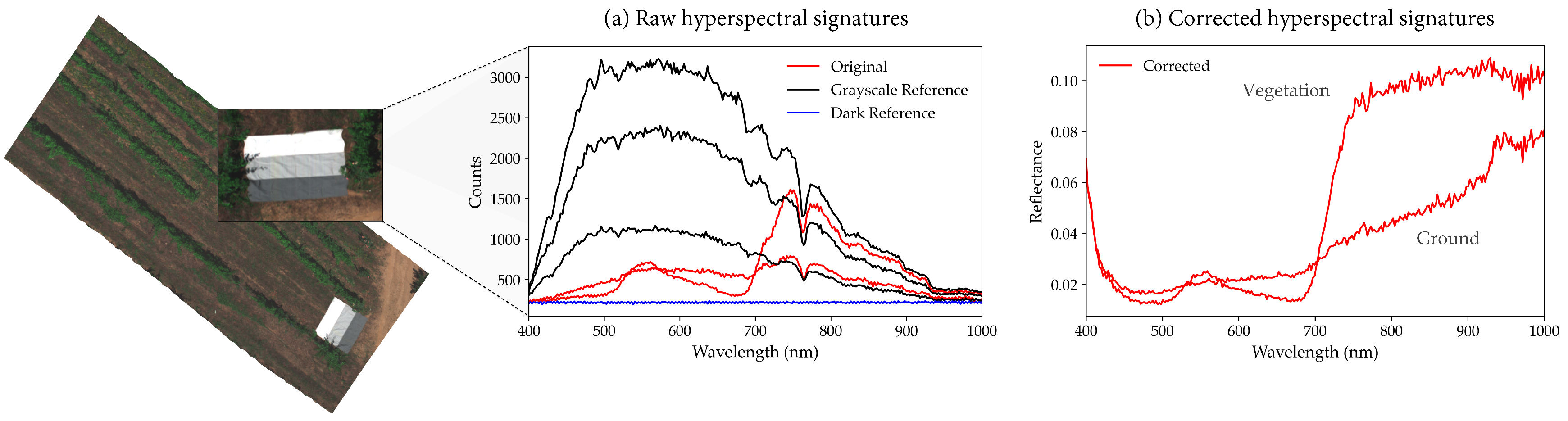
In a similar way to geometric distortions, radiometric anomalies can also be fixed with software tools provided by the hyperspectral manufacturer. The aim is to convert the digital numbers (DNs) of the sensor to radiance and reflectance of Earth’s surfaces, regardless of acquisition conditions. Therefore, the latter result must be applied to deep learning techniques for their implementation over any hyperspectral dataset. The coefficients required for this correction are generally calibrated in the laboratory, but they may vary over time [14], which may affect the radiometric correction. Grayscale tarps, whose reflectance is known, can be used to support this process and perform linear interpolations to calibrate the acquired DNs [19] using the empirical line method [9,20]. To perform the linear interpolation for the radiometric correction, it is necessary to have dark and gray/white references, which are usually obtained from isotropic materials that have a grayscale palette and exhibit near-Lambertian behaviour [12,21,22]. An alternative approach is to acquire radiance samples, which can be used with fitting methods such as the least-square method to transform DNs.

2.2. Hyperspectral Transformation and Feature Extraction

In this section, we discuss the transformations that facilitate classification using traditional methods. Due to the extensive coverage of land by satellite imagery, it is uncommon for hyperspectral pixels to depict the spectral signature of a single material. Consequently, analyzing the surfaces visible in collected hyperspectral signatures is a prevalent topic in hyperspectral research. The problem is illustrated with $\rho =\mathit{MF}+ϵ$, where M is the spectral signature of different materials, F is the weight, $ϵ$ is an additive noise vector and $\rho$ is an $L\times 1$ matrix where L is the number of bands. Hence, the difficulty of finding a solution to M and F is lowered if M is fixed, i.e., the end-member signatures are known. Multiple end-member spectral mixture analysis (MESMA) was the initial approach taken, followed by the mixture-tuned matching filtering technique, which eliminates the need to know end-members in advance. This approach was further refined with the constrained energy minimization method, which effectively suppresses undesired background signatures.

The current state-of-the-art techniques for linear mixture models can be categorized based on their dependency on spectral libraries. Additionally, the level of supervision and computational cost also determine the taxonomy of methods [23]. For instance, Bayesian methods and local unmixing do not necessitate end-member signatures, although Bayesian-inspired approaches are less supervised and more time-intensive. Besides MESMA, other proposed methods that require spectral signatures are based on artificial intelligence (AI) techniques such as machine learning (ML) and fuzzy unmixing. The latter is less supervised but more time-consuming. In recent years, interest in deep learning (DL) has grown, with techniques such as autoencoders, convolutional neural networks (CNNs) and generative adversarial networks being utilized for training with synthetic data [24]. Non-negative matrix factorization (NMF) has also attracted attention as it can extract sparse and interpretable features [25]. Recently, state-of-the-art methods such as NMF have been combined with spectral information [26].

Besides discerning materials, the results of hyperspectral imaging (HSI) present a large number of layers that can be either narrowed or transformed, as many of them present a high correlation. Otherwise, the large dimensionality of HSI data leads neural networks and other classification algorithms to be hugely complex. Accordingly, the most frequent projection method is PCA (principal component analysis) [27,28,29], which projects an HSI cube of size $X\times Y\times \lambda$ into $D\times B$, where D has a size of $X\times Y\times F$, and B is a matrix such as $F\times \lambda$. In this formulation, F is the number of target features. Independent component analysis is a variation of PCA that not only decorrelates data but also identifies normalized basis vectors that are statistically independent [30]. Least discriminant analysis is another commonly used technique, but it is primarily applied after PCA to increase interclass and intraclass distance [28]. In the literature, it is also referred to as partial least-square discriminant analysis, mainly as a classifier rather than a feature selection method.

Instead of projecting features into another space, these can be narrowed into the subset with maximum variance according to the classification labels of HSI samples. There are many techniques in this field, including the successive projection algorithm, which reduces colinearity in the feature vector. The competitive adaptive reweighted sampling method selects features with Monte Carlo sampling and iteratively removes those with small absolute regression coefficients. Two-dimensional correlation spectroscopy aims to characterize the similarity of variance in reflectance intensity. Liu et al. [31] used the Ruck sensitivity analysis to discard bands with a value below a certain threshold. Agilandeeswari et al. [32] calculated the band entropy, vegetation index and water index for wavelength subsets, generating a narrower cube only with bands above three different thresholds. Finally, the work of Santos et al. [33] presents an in-depth evaluation of methods based on PLS regression. To this end, HSI data from olive orchards were first narrowed and then classified with LDA (least discriminant analysis) and K-nearest neighbors. In conclusion, the Lasso method [34] as well as genetic algorithms [35] showed the best performance with LDA.

2.3. Traditional Hyperspectral Classification

Deep learning methods have recently become the preferred approach for classifying hyperspectral imagery. However, earlier techniques relied on comparing the acquired data to reference reflectance shapes that were ideally measured in a laboratory. The primary objective of these methods was to measure the similarity between labelled and unlabelled spectral shapes. Spectral libraries, containing data measured from a spectrometer, were used for these comparisons [36]. These methods varied from the widely used Euclidean distance to more sophisticated techniques such as spectral angle matching, cross-correlogram spectral matching and probabilistic approaches like spectral information divergence [30]. In addition, error and colorimetric methods [37] have been investigated in previous studies.

2.4. Classification of Hyperspectral Imaging with ML and DL

This section reviews studies related to the classification of vineyard varieties using HSI. However, only a few studies address HSI classification over vineyard varieties; therefore, other state-of-the-art DL networks achieving high accuracy in HSI classification will also be reviewed. Note that our research investigates pixel-wise classification, and models aimed at semantic segmentation (e.g., encoder–decoder architectures) are omitted.

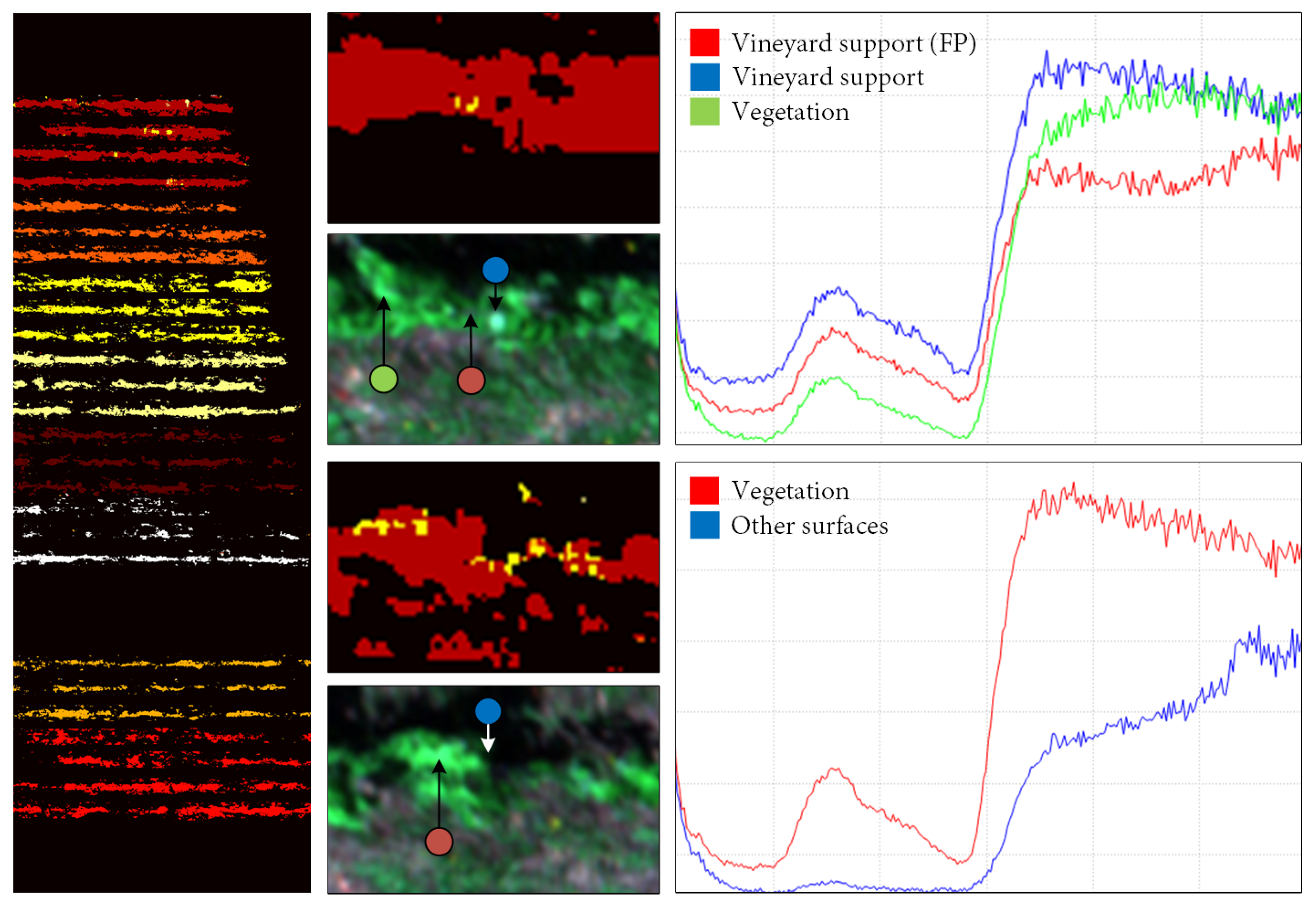
In previous grapevine classification studies, binary masks or grayscale maps were first extracted to distinguish soil, shadows and vineyards. Clustering, line detection and ML algorithms have been applied to segmenting vineyard rows [11,38,39,40,41,42], amongst which artificial neural networks (ANNs) stand out. Geometrical information from depth maps, DEMs, LiDAR data and photogrammetric reconstructions were also assessed [11,43,44,45], showing that this information improves the baseline performance. DL approaches for semantic segmentation and skeletonization algorithms have also been discussed [46,47]. Further insight into this field is provided by Li et al. [48].

Other vineyard classification studies operate with traditional methods and proximal hyperspectral sensing. In the work of Gutiérrez et al. [49], samples were selected by manually averaging the variety signature and filtering those with high correlation to such a signature. A support vector machine (SVM) and multilayer perceptron (MLP) were then trained with k-fold to distinguish thirty varieties (80 samples for each one), with the latter obtaining a recall close to one. Murru et al. [50] collected infrared spectroscopy data of five grape varieties and classified them using ANN with an overall accuracy (OA) of 85.3%. Similarly, Fuentes et al. [51] employed identical data types across sixteen grapevine cultivars, contrasting with colorimetric and geometric leaf features. Their classification methodology leveraged ANNs, yielding an OA of 94.2% by integrating morpho-colorimetric attributes. Kicherer et al. [52] presented a land phenotyping platform that segments grapes from the depth map and discerns between sprayed and nonsprayed leaves. To this end, several learning models were tested: LDA, partially least square (PLS), radial basis function (RBF), MLP and softmax output layer, with RBF and PLS showing the best results. Besides phenotyping, the following work is aimed at detecting diseases [53,54,55] and plagues [3]. Nguyen et al. [53] attempted to differentiate healthy and infected leaves with data obtained from land. They flattened the data processed by 2D and 3D convolutional networks and used them as input for random forest (RF) and SVM algorithms. They found that combining PCA reduction (50 features) and RF resulted in the best performance (97%), and RF improved SVM classification regardless of data reduction. However, it notably varies according to the case study; for instance, Wang et al. [56] reported that minimum noise fraction performed better in classifying crops over HSI. Another revised ML algorithm is gradient boosting for binary HSI classification over aircraft imagery [57], with an OA over 98% when discriminating algae.

Nevertheless, some of these applications formulate a binary problem where signatures of distinct classes significantly differ in scale and shape. Others operate with small datasets obtained on land via close sensing [58] or from imagery acquired at higher altitudes (hence showing more recognizable spatial features). For instance, a lightweight CNN composed of several inception blocks was also developed to classify up to 15 plant species [58] using multispectral images with a size of at least $200\times 200$ pixels. The authors found that the best results were achieved using a combination of six RGB and near-infrared features, with an accuracy of 94.7%. The use of PCA with only six features achieved an accuracy of 88%. Nezami et al. [59] also applied a 3D CNN to classify three tree species using both hyperspectral and visible imaging as well as canopy height models as input, with an OA below 95%. While it performs well over notably different materials, the network is not complex enough to discriminate similar hyperspectral signatures. On the other hand, transfer learning, attention-based and residual models are commonly observed in the literature [60]. Zhou et al. [61] delved into the realm of CNNs trained on distinct domains for satellite HSI classification, augmented with few-shot learning techniques. Although not yet attaining state-of-the-art performance, this approach showcased promise in expediting training procedures [62].

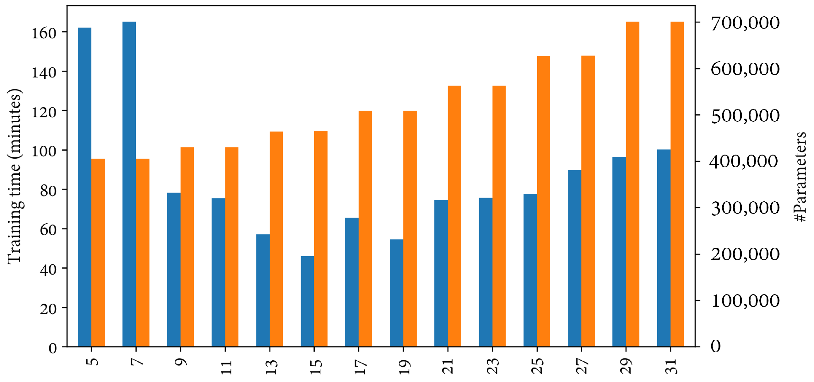
Regarding DL, the classification of satellite HSI is more frequent than using UAV imagery. Among previous works, the top-performing models based on their OA are discussed below. Zhong et al. [63] published an HSI dataset and proposed a simple CNN with conditional random field (CRF) to extract spatial relations among data, even with the presence of gaps. They obtained an OA of 98% and 94% over their own HSI dataset. Moraga and Duzgun [64] presented an inception-based model with parallel convolutional pipelines of increasing size, achieving near-perfect classification. Chakraborty and Trehan [65] proposed the SpectralNet model, which combines wavelet decompositions with a traditional convolutional path (OA: 98.59–100%). HybridSN [66] included both spectral–spatial and spatial feature learning using 3D and 2D convolutional layers (OA: 99.63–100%). Later, a network based on residual blocks and spectral–spatial attention modules with varying architecture (start, middle and ending ResBlock) (OA: 98.77–99.9%) was presented [67]. Lastly, the A-SOP network [68] proposed a module composed of matrix-wise operations that output a second-order pooling from the attention weights after extracting the first-order features (OA: 98.68–100%). Similar to Moraga and Duzgun’s work in 2022, the FSKNet model employs a combination of 2D and 3D convolutional layers with an intermediate separable convolution to reduce training latency while achieving comparable overall accuracy results. It achieves an OA above 99% with significantly fewer parameters and a shorter training time. Finally, other approaches have gained attention lately, such as contrastive learning, multi-instance segmentation and transformer networks [69] (e.g., using the BERT architecture [70] with an OA above 99%).

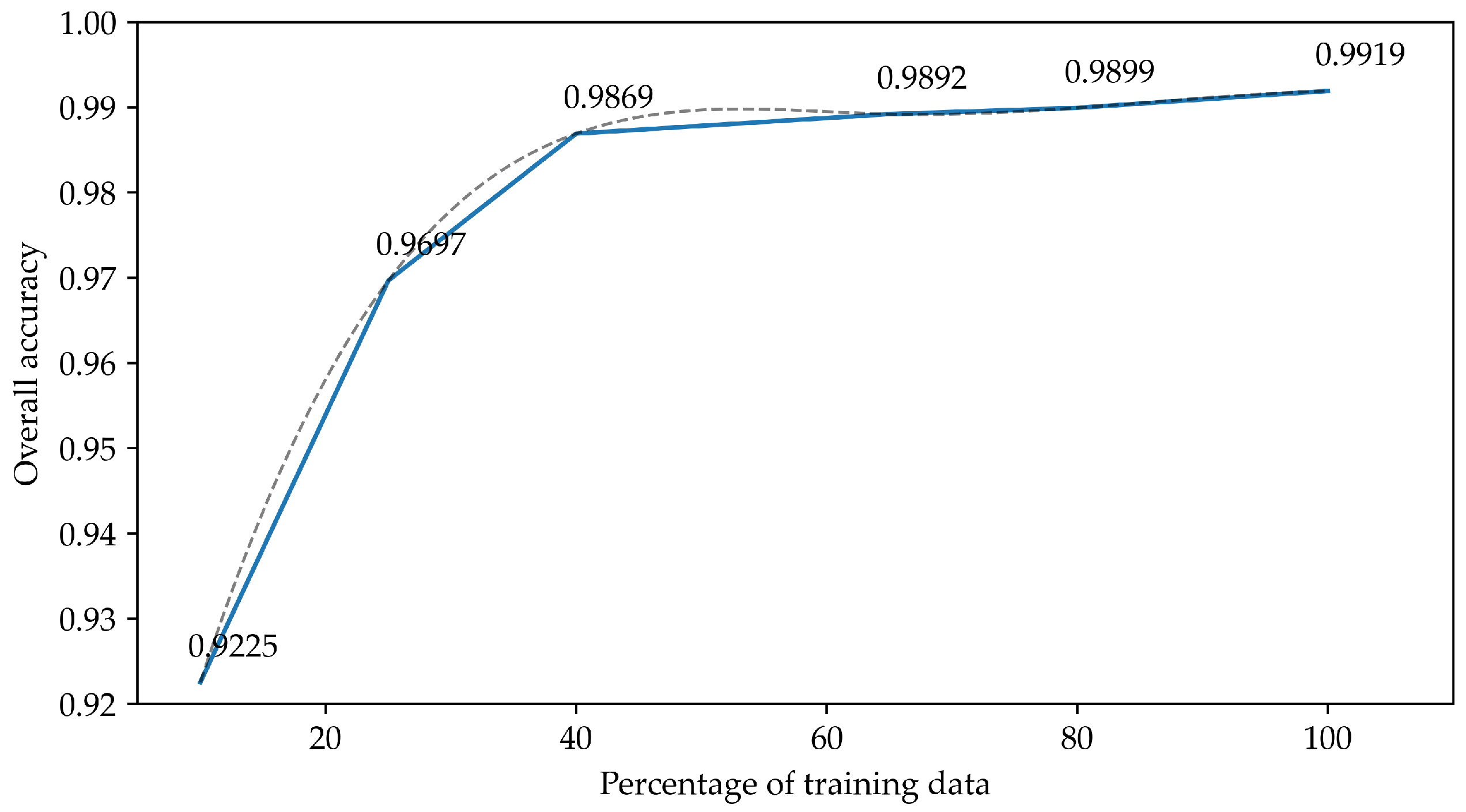
Although revised studies present outstanding results, most of them operate over satellite and aircraft imagery. These datasets are frequently less noisy and more curated than UAV images. Moreover, spatial features are not as relevant nor apparent in imagery obtained at a lower altitude, which is later subdivided into patches with low to no label heterogeneity. Indeed, we compare our method to numerous models to show that they underperform over UAV-based HSI.

3. Materials and Methods

The structure of this section is as follows: firstly, a brief explanation of the study area and sensors is provided. Next, the challenges of classifying vine varieties are introduced by the collected data. Subsequently, UAV imagery is utilized to differentiate between phenotypes of white and red root variants. To achieve this, a CNN architecture is proposed, which is evaluated against previously reviewed work with impressive OA results.

3.1. Study Area

The vineyards used as study areas in this work are situated in the northern region of Portugal, specifically in Vila Real (Figure 1). Each vineyard plot is dedicated to either red or white grapevine variants, and each grapevine variety is cultivated in one or more contiguous rows. The names of the row varieties were visible at the ground level via human-made marks, and these were annotated for the individual classification of rows visible in aerial imagery. The first crop (a) extends over 0.1551 $\mathrm{h}\mathrm{a}$ and the second one (b) covers an area of 0.2814 $\mathrm{h}\mathrm{a}$.

Figure 1. Overview of the areas surveyed using UAV hyperspectral imaging for the classification task. Two different vineyard crops are depicted according to their main variety: (a) red and (b) white.

3.2. Material

A Matrice 600 Pro (M600) hexacopter (DJI, Shenzhen, China) equipped with a Nano-Hyperspec from Headwall was used for the UAV flight. A Ronin-MX (DJI, Shenzhen, China) gimbal was employed to minimize geometric distortions in HSI acquisition. The lens had a focal length of 12 $\mathrm{m}\mathrm{m}$, covering 21.1°. The HSI swaths had 270 spectral bands and a width of 640, with the height depending on the flight plan. The spectral range went from 400 $\mathrm{n}\mathrm{m}$ to 1000 $\mathrm{n}\mathrm{m}$, with a uniform sampling of 2.2 $\mathrm{n}\mathrm{m}$ that increased to 6 $\mathrm{n}\mathrm{m}$ at half maximum. The UAV’s location was captured at different timestamps using two positioning antennas, and angular data were recorded using an inertial measurement system (IMU). The flight was planned using Universal Ground Control Station at an altitude of 50 $\mathrm{m}$ with a 40% side overlap. The red and white varieties were surveyed with 8 and 5 swaths, respectively. Table 1 provides a summary of the number of samples of each grape variety.

Table 1. Summary of acquired information regarding different grapevine varieties. For each variety, the number of field rows and image pixels obtained by labelling UAV imagery is shown.

Grapevine Berry	Vineyard Variety	No. Field Rows	No. Pixels
Red	Alicante	3	58,680
	Alvarhelao	4	144,315
	Barroca	3	35,656
	Sousao	3	75,078
	Touriga Femea	3	36,114
	Touriga Francesa	3	71,547
	Touriga National	3	53,620
	Tinta Roriz	4	67,157
White	Arito Do Douro	1	92,432
	Boal	3	44,654
	Cercial	1	105,384
	Codega Do Ladinho	3	261,228
	Donzelinho Branco	1	98,304
	Malvasia Fina	3	242,412
	Moscatel Galego	1	101,885
	Nascatel Galego Roxo	1	92,432
	Samarrinho	1	77,229
Total			1,658,127

3.3. Preprocessing of Hyperspectral Data

This section briefly describes the process of obtaining reflectance data from raw hyperspectral imagery, illustrated in Figure 2. The hyperspectral data were collected using a drone and processed using Headwall SpectralView™ software (v3.1.5.1, Headwall Photonics, Inc., Bolton, MA, USA). Several swaths were captured for each study area, and a white sample was marked from the white area in a grayscale tarp, while a dark reference was obtained by collecting a hyperspectral sample with the lens cap on before the flight. The sensor exposure and frame period were adjusted before the flight by pointing at a bright reference to avoid clamping samples from white surfaces. The white and dark references were then used to convert the raw data to reflectance. The ortho-rectified swath in Figure 2 was obtained using high-resolution DEMs (25 $\mathrm{m}$) from Copernicus’s observation program [71] and the drone’s GPS and IMU data. However, non-ortho-rectified swaths were used for the analyses presented in this paper to work with smaller image sizes and avoid distorting the hyperspectral signatures.

Figure 2. Conversion of (a) hyperspectral DNs into (b) reflectance using white and dark references. The three grey levels are sampled in (a).

3.4. Transformation of Hyperspectral Data

The analysis of the corrected reflectance data involved several steps to observe and differentiate the spectral signatures from different varieties. Initially, PCA was employed to explore the clustering patterns, extracting 50 features and narrowing them to three components using uMAP (uniform manifold approximation and projection for dimension reduction) [72]. As a result, Figure 3 shows that there are no clear distinctions between different varieties.

Figure 3. Three-dimensional distribution of hyperspectral samples from 17 classes, obtained by narrowing 50 components calculated with PCA into three components estimated by uMAP.

To determine the most suitable feature transformation algorithm for the collected HSI data, we evaluated four algorithms: NMF, PCA, FA and LSA. These were selected because they do not require the sample labels for their execution and therefore can work over not-yet-observed data. Additionally, LDA was included in these tests despite requiring the labels. Note that the evaluated samples simply consist of 140 bands after discarding the first and last layers, which are typically noisier. These were tested in isolation rather than using their neighborhood. For each algorithm and varying numbers of features, from 5 to 95, two tests were performed. First, the distance-based separability measure (DSI) was computed using the transformed manifold [73]. Subsequently, an SVM model was trained to predict the labels of the transformed samples. Through this evaluation, it was determined that FA outperformed the other algorithms in terms of both metrics, especially with more than thirty-five features. The results of these experiments are summarized in Figure 4, which supports the use of FA with forty features in the following sections.

Figure 4. Results of experiments conducted to compare different feature transformation algorithms with different numbers of components. PCA, FA, NMF and LSA (truncated SVD) are evaluated using the DSI metric and the OA obtained by training an SVM model. The default DSI and accuracy are obtained from the original data with 140 features.

Furthermore, feature transformation algorithms, such as FA, help to perform material unmixing to make the processing more robust against different background surfaces, including soil, low vegetation and other human-made structures. Pixels from UAV-based hyperspectral swaths depict more than one material. Therefore, the classification of these data ought to work under different kinds of surfaces. As proposed in recent work, material unmixing could be performed with NMF. To this end, hyperspectral swaths in reflectance units could be flattened to 1D ($n\leftarrow h · w$) with a dimensionality of $n\times m$, where m is the number of features. Then, this flattened vector could be transformed into weight ($W_{n\times c}$) and component ($C_{c\times m}$) matrices, where c is the number of target surfaces (end-members). However, the number of materials visible in a single image (or vineyard varieties plus ground) is not known in nature. Hence, material unmixing with an unknown number of target materials is suited for the classification of significantly different signatures rather than for performing fine-grained classification as in our case study. On the other hand, the feature space can be transformed and narrowed to a few more representative features instead of unmixing materials. In this regard, FA is also aimed at decomposing A into $W\times C+\mathsf{\Theta }$ without the non-negative restriction, with $\mathsf{\Theta }$ being the measurement error [74]. For this reason, FA was proven to be highly suitable to our case study, beyond outperforming the rest of the feature transformation methods in terms of separability and classification accuracy using an SVM model.

3.5. Automated Training

The classification of vineyard varieties with UAV data can be hardly approached with 1D algorithms due to the high similarity of spectral signatures. This shortcoming was already observed in Figure 4, where SVM did not perform well for any number of features (OA below 50% in every case). In this section, a method based on deep learning is described to classify 3D hyperspectral patches. In this section, the proposed method is tuned to achieve a high generalization performance.

3.5.1. Dataset

The hyperspectral imagery used in this study was collected on 28 July 2022, when all reported grapevine varieties were observed to be in a mature phenological stage. This ensured consistency and comparability across the surveyed plots, despite variations in the phenological cycles of different grapevine varieties.

Once radiometrically corrected, hyperspectral swaths were manually labelled as depicted in Figure 5 to distinguish different vineyard varieties. The Normalized Difference Vegetation Index (NDVI) was first extracted to differentiate vegetation from the ground, and images were then thresholded to create a binary mask from each swath. Following this, these binary masks were annotated with Sensarea [75] by marking each row with a different polygon and color, according to the variety annotated via human-made marks at the ground level. Some rows were marked with more than one polygon in order to avoid annotating small vegetation clusters that do not belong to vineyards but to small vegetation. For this reason, different polygons were labelled with the same colors, also because some varieties were repeated in several rows. According to this, Table 1 shows the number of collected samples for each variety and the number of cultivated rows.

Figure 5. Workflow for manually labelling HSI swaths. First, the false RGB image is displayed. Then, the NDVI is extracted, followed by thresholding and marking with polygons using the Sensarea software. Finally, a Boolean operation, AND, is performed between the polygon and binary masks to obtain the final labelled regions.

HSI cubes and masks were then split into 3D patches whose size is a matter of discussion in Section 4. Dividing the hyperspectral swaths into patches for classifying pixels using their neighborhood helps to partially suppress noise. Individual pixels are not substantial enough by themselves; instead, aggregations learned by kernels help to mitigate the noise. The window size used in this study is $23\times 23$ by default, whereas previous work used patches whose x and y dimensions range from 7 [67] to 64 [65]. Only [58] reported patches of much larger dimensionality ($200\times 200$) for multispectral images. The larger the patch, the deeper can be the network, though it also increases the number of trainable weights, the training time and the amount of data to be transferred into/from the GPU. Configurations using larger patch sizes are more suited to images with notable spatial features, such as close-range imagery [58], whereas ours ought to be primarily discerned through spectral features.

Instead of inputting the label of every patch’s pixel, they were reduced to a single label corresponding to the centre of an odd-sized patch. Thus, the classification was performed per pixel rather than through an overall semantic segmentation. Based on this, the hyperspectral samples were processed using the following steps: (1) separating the training and test samples at the outset, (2) fitting the FA and standardization only to the training samples to emulate a real-world application and (3) transforming both the training and test samples using the fitted models (see Figure 6). Standardization was utilized to eliminate the mean and scale reflectance to unit variance. By employing this approach, the CNN restricted the range of input HSI values, although the initial values were expected to differ due to various sensor exposures, frame periods and environmental conditions across different flights. Regarding feature reduction, spectral bands were transformed and narrowed to $n\leftarrow 40$ with FA. None of the fitted models requires the pixel’s labels and thus are very convenient for their application in new unlabelled areas. The resulting dataset is composed of 542,167 and 1,115,960 patches for red and white varieties, which were split into training (68%), validation (12%) and test (20%) subsets. With this partitioning, a total of 368 k samples were used for training on red varieties, and 758 k were applied to white variety classification.

Figure 6. Overview of dataset preparation. First, a binary mask was generated using the NDVI and rows were organized into different groups to distinguish vineyard classes. Once pixels were processed as described in Section 3.3, both reflectance and labels were split into patches. The signatures on the right side show the original and transformed reflectance, including the variance per feature. Blue lines show the averaged ground spectral signature, whereas orange represents the pixels labelled as vegetation.

3.5.2. Implementation

To make this paper self-contained, a brief introduction about DL is detailed in this section. Firstly, deep learning refers to layered representations that evolve in a learning process where they are exposed to input data. Typically, the depth of these models is large enough to automatically transform data and learn meaningful representations of data. Despite these models being able to work over any kind of structured data, even 1D, it is here proposed that one’s pixel neighborhood may help with the phenotyping problem. Convolutional neural networks (CNNs) have achieved remarkably good results in the computer vision field. Convolutions are designed to learn local features, rather than global, by applying element-wise transformations while sliding over input data. These are defined as rank-3 tensors defined by width, height and depth. The width and height determine how large the neighborhood of every element is, whereas the depth is the number of different learned filters. Hence, a single filter is applied element-wise to compose a response map from input data, whereas the whole filter stack is known as a feature map. If several convolution operations are concatenated, these evolve from learning low-level details (e.g., edges) to high-level concepts. Since individual filters are applied element-wise, the learned patterns are invariant to the position within the image [76]. However, kernels may not be applied for every element. Instead, information can be compressed using steps greater than one, also known as the stride value. Another key concept in CNN is that not every node is connected, thus partially tackling the overfitting problem. Training and test errors ought to remain similar during training, which implies that the network is not learning the training data (overfitting) or generalizing excessively (underfitting). To avoid both situations, the capacity of the model must be tuned in terms of complexity to generalize and reach low training errors.

Trainable CNN layers are typically defined by a matrix of weights and biases applied over input data, $f(x;w,b)$, with f being an activation function that allows the solving of nonlinear problems. In this work, ReLU and Leaky ReLU are applied to tackle the vanishing gradient problem, together with batch standardization. The latter operations work similarly to the standardizer applied as a preprocessing stage. On the other hand, w and b are updated during training to minimize a loss function comparing ground-truth and predicted values for supervised classification. This is performed by an optimizer that changes these trainable parameters using the error gradient scaled by the learning rate, $\eta$. The greater the $\eta$, the faster the convergence is achieved, though it can also lead to significant oscillations. This process is known as gradient descent (GD) [77]. As faster convergence may be necessary at the beginning, the decay and momentum concepts were introduced to downscale $\eta$ during training, thereby omitting abrupt changes.

Besides convolutions and normalization, there exist other layers to narrow data, avoid overfitting and output probabilistic values. The pooling operations, with max and average being the most popular, are aimed at downsampling input data. Dropout layers are used as a mechanism to introduce some noise into the training by zeroing out some output values, thus getting rid of happenstance patterns. Weight regularization also seeks to make the model simpler by forcing the weights to be small. Finally, the output units of the model are aimed at transforming features to complete the classification task. For a multilabel problem, the softmax represents the probability distribution of a variable with n possible values.

The kind of problem and label representation is coupled with the cross-entropy function measuring the error. Sample labels were not hot-encoded to reduce storage footprint, and therefore, a sparse categorical cross entropy as defined in Equation (1) is used for training in a multiclass problem. Otherwise, hot encoding requires transforming labels into binary vectors of size c that activate the indices of the sample label(s), with c being the number of unique labels.

$$L_{\mathit{CE}}=-ln\left(\widehat{y}\left[y\right]\right)$$

(1)

where $\widehat{y}$ is the model’s output as a vector of size c with $\widehat{y}\left[i\right],i\in \left[0,c-1\right]$ indicating the probability of the sample to belong to the i-th class, and y is the ground truth given by an integer value.

3.5.3. Architecture and Training

Several architectures were checked over both datasets, transitioning from networks with a few layers to the network proposed in Figure 7. Hyperparameter tuning was also used to define the best values for dropout, activation and convolutional layers, including the number of filters, the percentage of zeroed weights, the gradient of Leaky ReLU activation and the final activation.

Figure 7. Scheme of the proposed CNN, highlighting four different parts as well as the structure of inception blocks.

The input of the network is a single patch of size $23\times 23\times 40$. Moreover, the attention-based kernel of [68] is included as the first layer in order to discriminate representative spatial–spectral low-level features from the starting data. In this manner, it is able to extract spectral features without neglecting spatial ones within each patch. The first operation in the attention-based thread is to normalize the data, from which the kernel will learn the weights. Such a kernel is a correlation matrix that learns the cosine distance between the central pixel and the neighbors. Then, learned weights are normalized through a softmax function that is shown to provide better convergence. With this in mind, the attention-based thread can be formulated as follows:

$$\begin{array}{cc}\hfill {{\mathcal{P}}_{\mathit{norm}}}^{M^2\times B}& \leftarrow l_2\left({\mathcal{P}}^{M^2\times B}\right)\hfill \\ \hfill {\mathcal{S}}^{M^2\times M^2}& \leftarrow \left[{{\mathcal{P}}_{\mathit{norm}}}^{M^2\times B}{\left({{\mathcal{P}}_{\mathit{norm}}}^{M^2\times B}\right)}^{⊺}\right]\hfill \\ \hfill {{\mathcal{S}}_{central}}^{M^2\times 1}& \leftarrow {\left[{{\mathcal{S}}_{\frac{M}{2}}}^{M^2}\right]}^{⊺}{\mathcal{K}}^{M^2\times 1}\hfill \\ \hfill {\mathcal{SA}}^{M^2}& \leftarrow {\mathcal{S}}^{M^2\times M^2}{\mathcal{K}}^{M^2\times 1}+{\mathcal{B}}^{M^2\times 1}\hfill \\ \hfill {{\mathcal{P}}_{\mathcal{SA}}}^{M^2\times B}& \leftarrow \mathit{softmax}\left({\mathcal{SA}}^{M^2}\right) · {\mathcal{P}}^{M^2\times B}\hfill \end{array}$$

where $l_2$ refers to L2 normalization, ${\mathcal{P}}^{M^2\times B}$ is a 3D patch resized from ${\mathcal{P}}^{M\times M\times B}$, $\mathcal{S}$, ${\mathcal{S}}_{\mathit{central}}$ as well as $\mathcal{SA}$ are intermediate states, and ${\mathcal{P}}_{\mathcal{SA}}$ is the result that is later concatenated with the original form. From here, the result is concatenated in z with the original inputted data. Unlike in [68], this approach communicates two data blocks to the following layers: (1) discriminative spatial–spectral features, mainly for areas with high label heterogeneity, and (2) the original data for areas in which previous features are not that relevant.

Then, two similar blocks are included as Part II and Part III in Figure 7. Both share the same structure: inception block, normalization, activation and dropout. This is a frequent follow-up of convolutional layers [68,78], with dropout being greater (0.4) for middle layers than the last and initial layers (0.2). Instead of using max-pooling to downsample the network, strides of size 2 in convolutional layers were observed to perform better. These blocks are particularly well suited to our case study, as variations in flight altitude and image resolution are common among different observations. Consequently, employing inception blocks with kernels of varying sizes demonstrates robust performance against these uncertainties. The network specifications are shown in Table 2.

Table 2. Layer specifications of the proposed network. Inception blocks are simply named, but their layers are not expanded here to make this table more readable.

Part	Layer	Kernel Size	Strides	Output Size
I	Input			23 × 23 × 40
	Spatial attention			23 × 23 × 40
	Concatenate			23 × 23 × 80
II	Conv2D	1 × 1	1	23 × 23 × 16
	Conv2D	3 × 3	2	12 × 12 × 16
	Leaky ReLU ($\alpha \leftarrow 0.1$)			12 × 12 × 16
	Batch normalization			12 × 12 × 16
	Dropout (0.2)			12 × 12 × 16
III	Inception v2		1 (Conv2D $1\times 1$), 2	6 × 6 × 96
	Batch normalization			6 × 6 × 96
	Leaky ReLU ($\alpha \leftarrow 0.1$)			6 × 6 × 96
	Dropout (0.4)			6 × 6 × 96
IV	Inception v2		1 (Conv2D $1\times 1$), 2	3 × 3 × 288
	Batch normalization			3 × 3 × 288
	Leaky ReLU ($\alpha \leftarrow 0.1$)			3 × 3 × 288
	Flatten			2592
	Dropout (0.2)			2592
V	Softmax			17
No. trainable parameters: 562,227.
No. non-trainable parameters: 768.
No. parameters: 562,995.

The inception block was first proposed by [79], which consists of a module with four parallel layers that are later concatenated: convolutional layers with different kernel sizes (1 for spectral features and 3 and 5 to obtain aggregations from surrounding pixels) and a max-pooling layer that works directly over input data. Accordingly, a response map with a large number of filters is obtained. The importance of each of them is determined by the following layers that will again downsample data. However, at the time, this layout was considered to be prohibitive if the input layer had a large number of filters, especially for kernels of larger size. Therefore, $1\times 1$ convolutions aimed at reducing data were attached before each one of the inception threads (max-pool and convolutions with $\kappa >1$). In this work, both proposals are used: the naïve is checked in the experimentation to increase the network’s capacity, whereas the second is part of the proposed network. The latter compresses spatial data even more and is then connected to the network output.

Finally, the model is fitted with training data, and its performance is assessed with validation samples. For supervised problems like ours, data are composed of both samples and ground truth. In this work, the training samples were split into several sets according to the hardware limitations, and the model was iteratively trained during a significant number of iterations ($\epsilon \leftarrow 500$). Besides mitigating storage limitations, this leave-p-out cross-validation also helps to generalize by not training over the complete dataset. Furthermore, each one of these clusters is further split into small batches during a single iteration. The batch size must be large enough to include a balanced representation of samples. In this work, the batch size was set to $2^{10}$. This phase can be terminated early if no improvements are observed during $t\leftarrow 20$ epochs. A summary of the hyperparameters used in this study can be found in Table 3.

Table 3. Hyperparameters used during training.

Hyperparameter	Value
Patch size	23
Patch overlapping	22
Batch size	1024
Epochs	500
Learning rate	$1^{-5}$
Number of training splits	9
Transformations per split	2
Optimizer	RMS propagation
Loss function	Categorical cross entropy
Training split	0.68
Validation split	0.12
Test split	0.2

3.5.4. Data Sampling and Regularization

It can be observed from Figure 8 that the dataset is not balanced. The number of vineyard rows differs in length and so does the number of examples for each variety. Instead of generating new feasible batches by upsampling, a subset was obtained with different techniques. The objective is not to equalize the number of samples for every variety but rather to make it more balanced. Accordingly, the subsampling is performed by determining how many groups are downsampled; the larger it is, the more balanced the dataset becomes at the expense of reducing the number of hyperspectral samples. In this regard, Figure 8 compares the original distribution observed in a training batch and the utilized downsampling technique. Besides balancing the dataset, which is split into several batches to make it fit in the GPU, the CNN is watched with a callback that saves the current best model and prevents saving an overfitted model.

Figure 8. From top to bottom: initial distribution of samples per label and after using the proposed narrowing, with only three groups being downsampled.

Batches were probabilistically ($\mathcal{P}\leftarrow 0.1$) transformed by performing rotations and orientation flips so that learned features are invariant to the flight’s positioning conditions. With this approach, each batch of the training dataset was processed twice, each one with a different random seed, and therefore, differently transformed patches. Hence, the regularization was controlled by the proposed downsampling and transformation sequences. Several considerations were also taken into account during the CNN design: (1) the CNN must not have a large number of trainable parameters to avoid overfitting and a sufficient number to cope with underfitting, and (2) dropout layers were included to randomly reset some output weights and thus lead to proper generalization.

4. Experimentation and Analysis

The effectiveness of the proposed network is evaluated in this section. To this end, the classification experiments are jointly performed over various hyperspectral swaths of both surveyed areas. Results are presented in terms of overall accuracy (OA), average accuracy (AA), statistical kappa ($\kappa$) and f1-score. The first shows the percentage of correctly classified samples, the AA represents the average class-wise accuracy, the $\kappa$ coefficient is the degree of agreement between the classification results and the ground truth and, finally, the f1-score measures the model’s precision by leveraging both precision and recall metrics. Several representative neural networks are compared with our method: LtCNN [58], JigsawHSI [64], SpectralNET [65], HybridSN [66], Nezami et al.’s [59] and A-SPN [68]. From these, only a few address airborne sensing imagery [58], and the rest are focused on satellite data. Hence, several considerations must be addressed: (1) some of these approaches apply different transformations to the input data and (2) the number of spectral bands also differs from our HSI device. Therefore, the preprocessing pipeline was selected as the one providing better performance over our input data, either our pipeline or the one proposed in the reference work. However, FA showed a higher performance for every network if input data were transformed according to this fitting method rather than the following:

• Nezami et al. and LtCNN used the corrected reflectance with no preprocessing.
• JigsawHSI used PCA, FA, SVD and NMF with 9–12 final features.
• LtCNN and HybridSN used PCA to transform reflectance with $n\leftarrow 6,30$ components, respectively, whereas n is unknown for A-SPN.
• SpectralNet used FA with only three features.

Regarding implementation, all the tests were performed on a PC with AMD Ryzen Threadripper 3970X 3.6 GHz, 256 GB RAM, Nvidia RTX A6000 GPU and Windows 10 OS. The proposed CNN as well as the compared networks were implemented with Keras (version 2.10.0) and TensorFlow (version 2.10.1) in Python. CUDA 11.8 and CuNN 8.6 were installed to reduce the fitting time. Not every network from previous work could be applied as published; for example, LtCNN is designed for large image patches ($200\times 200$), and thus, convolutional striding and max-pooling cannot be applied when patches reach a size of $1\times 1$. For LtCNN [29], kernel size and max-pooling’s strides were reduced as reflected in our repository (please, see Data Availability Statement).

4.1. Classification Results

Table 4 shows the overall results of our method in comparison with state-of-the-art networks for classifying HSI datasets. Most of them are considerably unstable due to operating with noisy UAV data rather than working with satellite imagery. In addition, the second-best-performing network is Nezami et al.’s [59], which is the only one checked against UAV datasets for discerning different tree species. Similar to ours, it is also a shallow CNN with only a few layers; however, convolutions are applied sequentially rather than operating with stacked features extracted from various parallel convolutions. The confusion matrix in Figure 9 shows the OA of the proposed network against any grape variety. Hence, classification over the majority of varieties shows uniform results, with most of them being close to 99%. Note that these percentages were rounded, and therefore, some of these results are below 99%, while others are above. When averaged, all these results lead to an OA of ≈$98.8$%, as shown in Table 4.

Table 4. Overall results in terms of OA, AA, f-1 and $\kappa$ coefficient with different methods. The best results for every metric were highlighted in bold.

Metric	Ours	LtCNN [58]	Nezami [59]	JigsawHSI [64]	SpectralNET [65]	HybridSN [66]	A-SPN [58]
OA	98.78 ± 0.15	74.33 ± 9.77	80.42 ± 0.59	73.89 ± 1.72	79.09 ± 0.55	63.46 ± 0.45	63.40 ± 0.69
AA	98.94 ± 0.09	73.09 ± 9.69	77.72 ± 0.43	73.55 ± 0.67	78.92 ± 0.29	63.04 ± 0.68	69.82 ± 0.49
Kappa	99.67 ± 0.05	91.15 ± 3.87	95.43 ± 0.28	90.27 ± 1.69	93.43 ± 0.15	89.68 ± 0.24	88.77 ± 0.31
f1	98.78 ± 0.15	73.86 ± 10.29	80.38 ± 0.61	73.00 ± 2.41	79.05 ± 0.56	63.10 ± 0.70	61.69 ± 0.96

Figure 9. Confusion matrix for classifying red and white varieties altogether.

4.2. Training Time and Network Capacity

The benchmark on the classification problem is relevant to show that training time is not excessive and that the proposed network does not have much more capacity than the problem warrants. Figure 10 shows that training and validation signatures are similar and therefore do not show overfitting or underfitting behaviours. Furthermore, the training AO and loss worsen as a new dataset is introduced, whereas the validation metrics remain similar. Along with this, the network is only parameterized by nearly 560 k parameters, while other state-of-the-art models exceed 10 million parameters (see Figure 11). The number of parameters is derived from the proposed architectures, using an input of size $23\times 23\times 40$. Note that the network of Lu et al. [29] was decimated in our experimentation with pooling operations of a lower size than proposed to adapt it to smaller patches. Finally, the response time for training the proposed network is below an hour, whereas others require up to several hours. Note that every available sample was used during training, instead of using strides; otherwise, the training time can be reduced. In conclusion, very shallow networks [68] or excessively deep ones [64] seem to struggle over a case study where spectral features have a greater weight in the inferring.

Figure 10. Training and validation accuracy and loss during training.

Figure 11. Response time for training the network (left axis) as well as the number of parameters (right axis) for every compared network, including ours [59].

4.3. Separability

The output of the proposed network can be assessed in terms of separability by removing the final dropout and dense layers. Data were transformed and flattened according to the network’s learned weights. It was subsequently embedded with uMAP [72] to compress high-dimensionality data into a few features, thus allowing us to visualize the new data representation. The same procedure can be followed over the original data to compare how the data manifold was uncrumpled. As shown in Figure 12, different labels were not perfectly unmixed, although the improvement in comparison to the starting representation is notable. To provide this result, the last densely connected layer was connected to uMAP fitting with $n=2$; hence, 2592 features were narrowed to two features to represent the embedding in a two-dimensional chart.

Figure 12. Clustering of samples according to the feature transformation performed by uMAP over (a) the starting hyperspectral features and (b) features extracted by the CNN before transferring it to the final softmax layer.

4.4. Impact of Window Size

The patch size is one of the most, if not the most, relevant parameters concerning the network architecture. Larger patches are assumed to also work, as irrelevant spatial features can be zeroed out. However, it also comes at the expense of increasing the training time. On the contrary, lower patches come at the risk of not being sufficient for classifying samples as accurately as performed by the proposed network. Figure 13 shows the whole battery of metrics obtained with patch sizes ranging from 5 to 31. According to the obtained results, patches were split with dimensionality 23 to balance network capacity and accuracy, despite a higher patch size achieving slightly better results. Accordingly, the highest patch size reached an OA of 99.57%, whereas the lowest reached 82.5% (size of 5). On the other hand, the selected dimensionality achieves an OA of 99.20%, thus leveraging network size and capacity. Figure 14 depicts the training time and network size as the patch dimensions increase. The number of training splits was calculated according to the patch size, and therefore, the lowest size had also a lower number of subdivisions. This led to a considerable time bottleneck in patch-wise transformations since they were performed in the central processing unit (CPU).

Figure 13. Overall accuracy obtained for patches of different sizes, from 5 to 31.

Figure 14. Training time (in minutes) and the number of parameters as the window size increases. The blue bars correspond to the left axis, representing training time, while the orange bars represent the number of parameters.

In conclusion, selecting a patch size implies leveraging several factors, including training time, network capacity and accuracy. Therefore, it must be selected according to the available computational resources, the image resolution and the minimum acceptable error rate. Using larger patches is safer but also increases the network capacity and training time. Hence, the relevance of selecting an appropriate patch size rather than the largest possible was proved in this experiment.

4.5. Ablation Study

The proposed network is intended to be validated in this section by removing and transforming some of the network features while the rest remain unchanged. The proposed changes are the following:

• Two convolutional layers were included before Part II to extract spectral and spatial features.
• Both inception blocks were modelled using the original structure [79]. The main difference between this architecture and ours is that the former stacks feature maps extracted with different neighborhood sizes, without downsampling data with $1 \times 1$ convolutions. Therefore, it increases the network capacity and training time.
• Only the first inception block was exchanged by a naïve version, as the one used in the previous experiment.
• The spatial attention layer was removed.

The obtained results are shown in Table 5. Removing the SA layer led to a slight decrease in performance, similar to exchanging the first inception block. Unsurprisingly, using the naïve version of the inception layer twice led to a significant performance decrease for every metric, as it kept transforming the spectral dimensionality in a deep layer. The second inception version also transformed spectral features but instead provided them as an additional layer (concatenation) that can be weighted according to their contribution to the output. Following this reasoning, swapping the first inception block with the first version of it did not involve a huge performance drop. Improvements to the proposed architecture over the third variant were very small and therefore may suggest that using either one of them does not offer great changes in performance. Similar results to the last setup were achieved by removing the spatial attention layer; it did not lead to a significant performance drop, though better and, especially, more stable results were obtained using the proposed network.

Table 5. Overall results in terms of OA, AA and kappa coefficient with different CNN schemes. The best results for each metric were highlighted in bold.

Metric	Ours	(a) With Initial Conv.	(b) Naïve Inception	(c) Naïve & Adv. Inception	(d) Without SA
OA	98.78 ± 0.15	98.04 ± 0.11	97.87 ± 0.29	98.51 ± 0.20	98.67 ± 0.23
AA	98.94 ± 0.09	98.21 ± 0.06	98.09 ± 0.25	98.90 ± 0.10	98.93 ± 0.11
Kappa ($\kappa$)	99.67 ± 0.05	99.43 ± 0.07	99.45 ± 0.08	99.58 ± 0.12	99.59 ± 0.04
f1	98.78 ± 0.15	98.04 ± 0.11	97.89 ± 0.28	98.52 ± 0.20	97.66 ± 0.22

4.6. Analysis of Errors

As observed in previous sections, our architecture achieved a high OA and AA. However, a margin for improvement can be found in the weaknesses of the labelling, transformation and classification pipeline. Instead of predicting randomly selected samples, another experiment is to predict every hyperspectral swath sample, thus allowing us to determine where errors are located within the study area. As observed in Figure 15, these errors are spatially clustered instead of being sparsed over the study area. If these are compared against the RGB mosaic of the hypercubes, errors are observed to belong to (1) small vegetation clusters, mainly from weeds mistakenly labelled as grapevine leaves, and (2) samples surrounded by ground or metallic vineyard supports. Note that these are hard to notice during the labelling since they present signatures similar to the target leaves and are surrounded by vegetation, thus hardening the definition of a geometrical shape for rapidly tagging whether it is relevant or not. Still, some errors are present in grapevine samples surrounded by ground and other surfaces that have a notable impact on the sample’s neighborhood, thus distorting the final probability. Note that boundary samples, i.e., those close to ground, have a signature that at least fuses the signatures of a grapevine variety and ground. Nevertheless, the weight of that specific variety in the signature may not be enough to tell apart varieties, thereby leading to mislabelling samples heavily surrounded by ground.

Figure 15. Errors observed in the classification of red varieties and the hyperspectral signature of a few samples concerning different surfaces. FP indicates a false-positive sample mistakenly labelled as vegetation during dataset preparation, since it reflects a human-made structure in the false RGB image. It led to a few prediction errors in close grapevine samples. However, it is not trivial to mask them out during dataset preparation.

4.7. Training over Satellite Imagery

The main shortcoming of the compared CNNs that focus on satellite imagery is that they obtain a poor performance over the proposed UAV datasets and vineyard varieties. Hyperspectral imagery from UAVs is noisier than satellite observations, with the spectral signature of the latter being more smoothed out. Therefore, previous work did not overcome noise in the classification of vineyards and most of them showed a poor performance. Only another architecture tested over UAV samples managed to reach an OA near 80%, whereas others showing worse results proposed huge networks with millions of parameters, thus overkilling the classification with a large training time.

To further evaluate the generalization capabilities of our proposed CNN, we conducted experiments using publicly available hyperspectral satellite imagery datasets [13]. These datasets, which are commonly used as benchmarks, vary in the number of spectral bands and label classes, with some datasets containing as few as nine classes and others up to sixteen. Similarly, the number of spectral bands differs from our imaging device. However, FA was fitted to obtain only 40 features per pixel, as proposed for UAV imagery and as is in the architecture of the network. According to the number of samples of each dataset, the batch size was adapted, as shown in Table 6. Every dataset had unlabelled samples which were removed from the training and test datasets to establish a fair comparison with previous work. Unlike our UAV datasets, labels in satellite imagery were imbalanced, with some of them having only a few dozen examples. Hence, balancing was not applied in satellite datasets to avoid levelling the rest of the classes with others that present scarce examples. As we did not intend to tune the network for satellite imagery, the learning rate remained as before, and the batch size was scaled according to the number of samples.

Table 6. Classification of HSI from satellite platforms in terms of OA and kappa coefficient ($\kappa$).

	Ours			State of the Art
Dataset	OA	Kappa ($\mathbf{\kappa }$)	Batch Size	OA	Kappa ($\mathbf{\kappa }$)	Reference Work
Pavia University	99.97 ± 0.01	99.99 ± 0.00	256	100 ± 0.00	100 ± 0.00	[64]
Indian Pines	99.53 ± 0.13	99.49 ± 0.14	64	99.93 ± 0.07	99.89 ± 0.10	[80]
Salinas Valley	100 ± 0.00	100.0 ± 0.00	256	100 ± 0.00	100 ± 0.00	[64]

Despite the differences in data characteristics between UAV-captured and satellite imagery, our CNN model performed robustly across all datasets. The model achieved OA, AA and $\kappa$ consistently above 99%, demonstrating its adaptability to different sources of hyperspectral data. Training times for satellite datasets were significantly lower compared to UAV datasets, attributed to the smaller size of satellite images. For instance, training on the Pavia University dataset required approximately 7 min, while the Indian Pines dataset took around 9.42 min to converge. Our model also handled imbalanced datasets effectively. For example, the Indian Pines dataset, which exhibits a high degree of class imbalance, did not substantially affect the classification performance, highlighting the model’s robustness. These results suggest that while our CNN is tailored for UAV imagery, it remains highly effective for hyperspectral satellite data, confirming its broad applicability in precision agriculture and beyond.

4.8. Training over Fewer Examples

Another conducted experiment was to train the proposed CNN with a lower amount of information. In this regard, the training was repeated to learn from a percentage of training samples ranging from 10% to 100% (of 68%). In Figure 16, it can be observed that the OA drastically goes to 92% with 10% of training data, although it is still able to learn relevant features to provide a high OA. It is hypothesized that as the number of training data increases, the number of learned spatial features is notably higher, whereas lower amounts of information are enough for learning spectral features that enable classifying samples from their neighborhood.

Figure 16. OA observed by training the proposed CNN network with a subset (percentage) of the training dataset. The dashed line represents the expected results for intermediate values.

4.9. Transfer Learning

Transfer learning has been widely studied to take advantage of trained networks with a notable capability of separating a variable number of classes. The underlying concept is that a network which has been successfully applied to one case study and has learned relevant features may be applied to another case study with a similar outcome. Nonetheless, it does not necessarily involve training the whole network, which typically has an extreme amount of parameters. Instead, some layers that learn more abstract features, presumably the first, are not trained; their weights are preserved, and deeper layers are trained to specialize in another application.

The objective of this section is to carry out several experiments to conclude whether weights learned over the classification of other UAV datasets can be exploited to make the training faster and even more accurate. This experiment was approached by using the publicly available WHU-Hi HSI datasets for classifying rural materials, including different vegetation crops [63]. These datasets are primarily designed for semantic segmentation applications, although the outlined transformation procedure can also be applied to them. It is important to note that these datasets have a lower level of detail (LOD) compared to ours, resulting in ground-truth masks that bear a closer resemblance to satellite imagery. Despite this reduced LOD, they have proven valuable in expediting the training process due to their smaller size. Conversely, the materials depicted in the WHU-Hi datasets exhibit significant dissimilarities from those present in our imagery. The ground-truth masks in these datasets appear smoother due to the lower LOD, leading to a heightened emphasis on spectral features, while spatial features contribute less significant information. Consequently, the learned weights from these datasets serve as initial weights, initiating a retraining process focused on acquiring spectral and spatial features from imagery collected with a high LOD.

Table 7 shows the outcome of this experimentation. Using previously trained weights considerably contributed to improving the metric results in comparison with the default weight initialization. By default, weights in Keras are initialized so that the variance is guaranteed to be similar across the network layers (Xavier initialization). Note that not every dataset evenly contributed to improving the results; the weights from the Han Chuan and Long Kou datasets seem to contribute better to separate hyperspectral samples.

Table 7. Classification of our HSI dataset with weights learned from WHU-Hi datasets and default Keras weights. The best results for each metric were highlighted in bold.

	Previously Trained Weights			Default Weights
Dataset	OA	Kappa ($\mathbf{\kappa }$)	f1	OA	Kappa ($\mathbf{\kappa }$)	f1
Han Chuan	99.10 ± 0.07	99.75 ± 0.01	99.10 ± 0.07	98.78 ± 0.15	99.67 ± 0.05	98.78 ± 0.15
Hong Hu	98.79 ± 0.13	99.68 ± 0.03	98.79 ± 0.12
Long Kou	99.09 ± 0.13	99.73 ± 0.07	99.09 ± 0.13

5. Discussion

Our study focused on evaluating the performance of a CNN for classifying grapevine varieties using UAV-based hyperspectral imagery. This domain presents unique challenges such as noisy imagery and highly similar hyperspectral signatures among different grapevine varieties. Selecting an appropriate CNN architecture is crucial to address these challenges. Shallow networks might fail to capture the intricate patterns within hyperspectral data, whereas deeper networks, while potentially more effective, are time-consuming and computationally intensive. They must also balance between spatial and spectral feature extraction, the latter being particularly crucial in vegetative materials. Previous studies largely concentrated on satellite imagery applications for CNNs, with a limited number of studies exploring data from UAVs [59]. UAV-based HSI tends to be noisier and more variable compared to satellite imagery, thus presenting additional difficulties in achieving high classification accuracy. Despite these challenges, our network achieved an accuracy of over 98.7% for classifying grapevine varieties from a UAV-based HSI dataset. Other comparable models showed a significant drop in performance when applied to this kind of imagery, often achieving only around 81% accuracy [59]. Our network’s efficiency is further underscored by its lower training time and fewer parameters (560 k), in contrast to other models that involve several million parameters [64].

A critical component of our approach was the preprocessing of reflectance data. Hyperspectral images typically include numerous bands, many of which may be redundant or irrelevant. Through feature reduction techniques, specifically factor analysis (FA), we effectively reduced the number of bands from 270 to 40 features. This reduction significantly decreased the model’s parameter count and response time while maintaining high classification accuracy. However, some mislabelled samples were identified, particularly in low-vegetation areas that were incorrectly labelled as grapevine varieties. Additionally, misclassifications due to the proximity of samples to other surfaces presented challenges when examined against false-color RGB imagery. Studies have highlighted the importance of preprocessing and feature reduction in hyperspectral data classification. For instance, as suggested by Alvarez-Vanhard et al. [10], preprocessing techniques significantly enhance classification accuracy in agricultural applications. Similarly, Khezrabad et al. [18] emphasize the benefits of feature extraction methods for hyperspectral imaging, which align with our use of factor analysis for band reduction. Hruška et al. [25] discuss the practical applications of UAV-based HSI for vineyard phenotyping, underscoring its potential in real-world scenarios. Our experiments demonstrated that pretraining the network on a different UAV hyperspectral dataset before fine-tuning it on the target dataset improved classification metrics. This pre-training enabled the network to better distinguish hyperspectral signatures, even when initially trained on different materials.

Our findings suggest that integrating spatial attention mechanisms and inception blocks within the CNN architecture significantly improves the model’s ability to extract relevant features, thereby enhancing its predictive power. This approach, combined with meticulous preprocessing, addresses the complexities inherent in hyperspectral data. The use of spatial attention mechanisms allows the network to focus on the most informative parts of the image, while inception blocks enable the extraction of multiscale features, both of which are crucial for handling the high-dimensional nature of hyperspectral data.

Moreover, incorporating a band-narrowing procedure reduced both storage requirements and the network’s computational footprint. This is particularly important in practical applications where computational resources and storage capacities may be limited. By demonstrating that a network with fewer parameters can still achieve high accuracy, our study provides a valuable contribution to precision viticulture.

6. Conclusions

The proposed CNN model utilizes cutting-edge techniques to effectively classify grapevine varieties. Our experiments highlighted the efficacy of spatial attention layers in improving classification results, and we conducted a thorough examination of inception blocks to determine their suitability for hyperspectral imagery. Importantly, our network demonstrated fast training times and a small footprint, achieving high overall accuracy across both UAV and satellite hyperspectral imagery datasets, even with limited training data. Additionally, pretraining the network with other UAV HSI datasets proved beneficial, albeit at the expense of increased training time. This model shows promise for accurately classifying a diverse range of grapevine varieties, potentially serving as a valuable tool for the wine industry to develop region-specific authenticity verification systems.

Future research endeavours will focus on exploring the classification performance of our proposed network at various phenological stages of grapevine growth. By collecting hyperspectral imagery at different stages of the phenological cycle, such as bud break, flowering, veraison and harvest, we aim to investigate how spectral signatures evolve and influence the network’s ability to accurately classify grapevine varieties. This comprehensive analysis will not only enhance our understanding of phenological impacts on classification outcomes but also contribute to the development of a more robust and adaptable classification framework for viticulture applications. Other already identified drawbacks, such as the time-consuming labelling stage, may greatly benefit from other data such as the DEM collected by the UAV to avoid some labelling errors and speed up this manual task.