Vulnerability of Wetlands Due to Projected Sea-Level Rise in the Coastal Plains of the South and Southeast United States

Abstract

Coastal wetlands are vulnerable to accelerated sea-level rise, yet knowledge about their extent and distribution is often limited. We developed a land cover classification of wetlands in the coastal plains of the southern United States along the Gulf of Mexico (Texas, Louisiana, Mississippi, Alabama, and Florida) using 6161 very-high (2 m per pixel) resolution WorldView-2 and WorldView-3 satellite images from 2012 to 2015. Area extent estimations were obtained for the following vegetated classes: marsh, scrub, grass, forested upland, and forested wetland, located in elevation brackets between 0 and 10 m above sea level at 0.1 m intervals. Sea-level trends were estimated for each coastal state using tide gauge data collected over the period 1983–2021 and projected for 2100 using the trend estimated over that period. These trends were considered conservative, as sea level rise in the region accelerated between 2010 and 2021. Estimated losses in vegetation area due to sea level rise by 2100 are projected to be at least 12,587 km², of which 3224 km² would be coastal wetlands. Louisiana is expected to suffer the largest losses in vegetation (80%) and coastal wetlands (75%) by 2100. Such high-resolution coastal mapping products help to guide adaptation plans in the region, including planning for wetland conservation and coastal development.

1. Introduction

Coastal wetlands are areas permanently or temporarily inundated by marine water. These areas provide habitat for terrestrial, aerial, and aquatic organisms [1]. They can mitigate the impacts of coastal storms and erosion [2,3] and store large quantities organic carbon [4,5]. The ecosystem services of coastal wetlands are considered essential [6].

Wetlands of the Atlantic and Gulf of Mexico coastal plain of the United States are a mixture of marshes, wet meadows, swamps including mangroves, and wet flatwoods [7]. Surface area estimates of these coastal wetland areas are difficult to find in part because of differences in how wetlands are defined and delimited, seasonal cover changes, and mapping quality [8,9].

Today, wetland mapping and monitoring is typically carried out using aerial and satellite remote sensing [10,11,12]. Land cover mapping in the United States is routinely done by the U.S. Fish and Wildlife Service (FWS), U.S. Geological Survey (USGS), and partners like the National Oceanic and Atmospheric Administration (NOAA), the U.S. Environmental Protection Agency (EPA), and various state agencies and research institutions. The federal efforts produce the National Wetland Inventory (NWI) and the National Land Cover Database (NLCD), which are updated every three to five years, respectively [13,14]. The Coastal-Change Analysis Program (C-CAP) from NOAA is the coastal expression of the NLCD. The NWI is produced from high-altitude airborne imagery, while the NLCD is derived using Landsat imagery at a nominal 30 m spatial resolution per pixel. Wetland mapping at higher spatial resolution is more accurate than coarser resolution products. For example, McCarthy et al. [11] classified wetlands in West Florida with WorldView-2 imagery at 2 m per pixel resolution and found higher accuracy in identifying forested wetland and upland vegetation compared to the NWI and C-CAP products. As more commercial satellite data become available, all agencies have started to develop land cover maps at spatial resolution finer than 10–30 m per pixel.

Major factors that are affecting wetland degradation and loss include human development (e.g., pollution, urban and other infrastructure, agriculture) and climate change [15,16,17]. In the United States, wetland areas decreased approximately 50% between 1780 and 2009. Nearly 50–60% of that loss was due to urban development and agriculture [8]. An important factor in planning for wetland conservation is sea-level rise (SLR). It has been estimated that 68% of coastal wetlands in 86 developing countries will be at risk if sea level were to rise 1 m [18]. Schuerch et al. [19] estimated global wetland losses between 0% and 30% by 2100 due to SLR alone. Osland et al. [20] estimated that in the United States, the highest potential for wetland loss by 2100 is in the states of Louisiana (29%), Florida (25%), North Carolina (10%), Texas (8%), and South Carolina (7%), considering a 1.5 m SLR scenario by 2100. Reed et al. [21] modeled three different scenarios of SLR for Louisiana in a 50-year period between 2015 and 2064 using a digital elevation model (DEM) at 30 m resolution. They estimated land losses, including wetlands, of between 3000 km² and 10,000 km² by 2064.

In this study, we refine the estimates of potential coastal wetlands losses in the south and southeast US using land cover maps and digital elevation models at much higher spatial resolution than the 30 m grid size previously available. This work is divided into three subsections: (1) development of a land cover map at high resolution (2 m pixels) of the coastal south and southeast United States; (2) estimation of areas of vegetation and wetland cover, including the distribution of wetland types in specific topographic bins; and (3) projected vegetation and wetland area loss given mean local SLR trends.

2. Materials and Methods

2.1. Study Area

This study focused on the coastal areas of the south and southeast United States (Texas, Louisiana, Mississippi, Alabama, and Florida) (Figure 1). All data products described below are accessible via the 3D-Wetlands app in Google Earth Engine (GEE), https://lizcanosandoval.users.earthengine.app/view/hr-land-cover-gulf-of-mexico, or the GitHub repository, https://github.com/luislizcano/3D-wetlands-app (accessed on 3 June 2024).

2.2. Satellite Data Processing

A total of 10,245 multispectral images spanning 2009 to 2018 collected with the WorldView-2 (8689) and World-View-3 (1556) satellites were obtained from the DigitalGlobe (Maxar) repository and screened for cloud cover. The WorldView-2 satellite sensor, launched in October 2009, provided data in eight spectral bands at ~2 m per pixel (

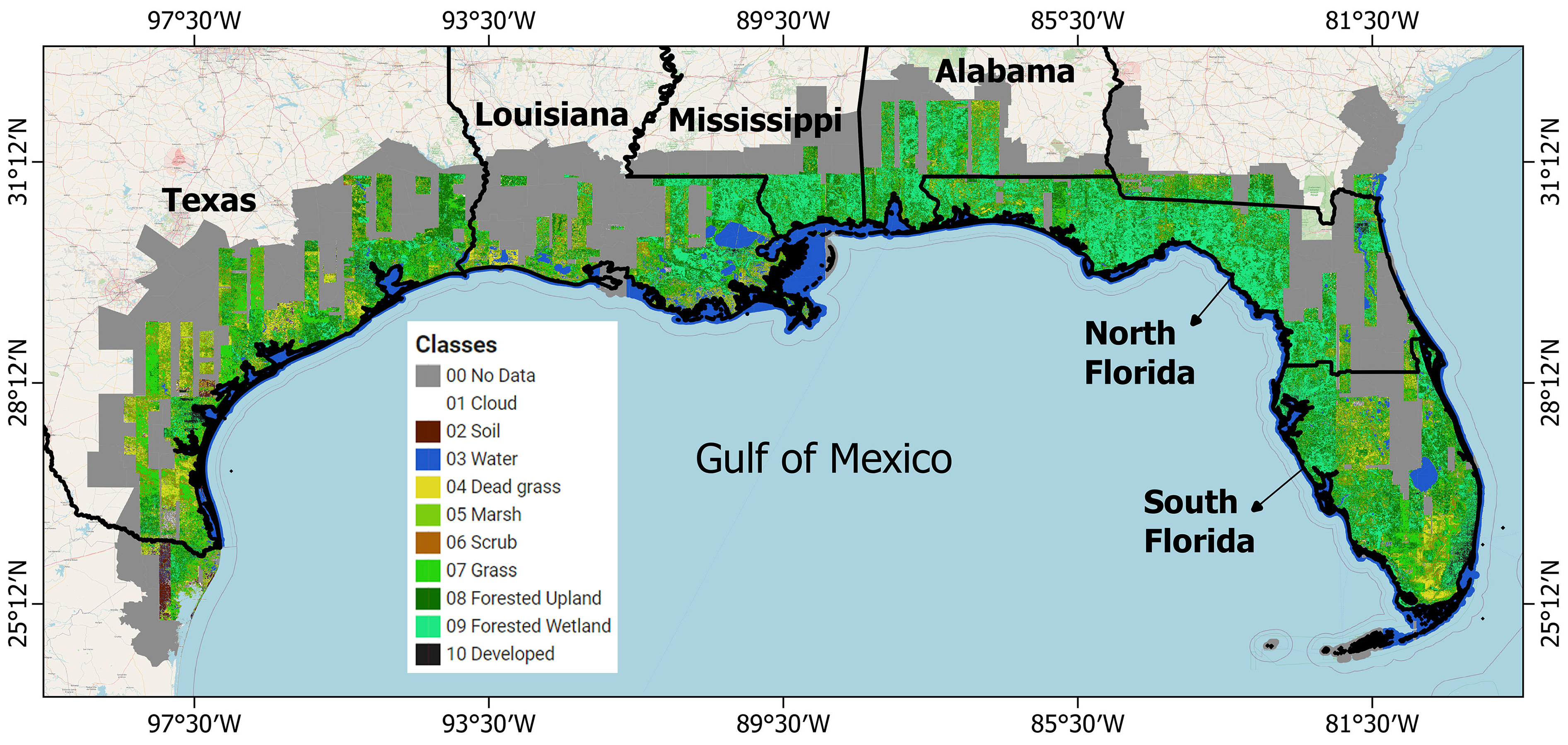
Table 1. WorldView-2 and WorldView-3 multispectral sensor specifications.

Band Name	Band Number	Center Wavelength (nm)	Band Coverage (nm)	Effective Bandwidth (nm)
WorldView-2
Coastal	1	427	396–458	47
Blue	2	479	442–515	54
Green	3	546	506–586	63
Yellow	4	608	584–632	37
Red	5	659	624–694	57
Red edge	6	724	699–749	39
NIR I	7	833	765–901	99
NIR II	8	950	856–1043	100
WorldView-3
Coastal	1	426	397–454	41
Blue	2	481	445–517	54
Green	3	547	507–586	62
Yellow	4	605	580–629	38
Red	5	661	626–696	59
Red edge	6	724	698–749	39
NIR I	7	832	765–899	100
NIR II	8	948	857–1039	89

). WorldView-3 was launched in August 2014, provided imagery in similar bands as WorldView-2, but from a lower orbit and at ~1.5 m per pixel. We only used WorldView-3 data in bands that matched those of WorldView-2 and did not use the eight short-wave infrared bands. We focused on the period 2012 to 2015 to derive land cover and used those maps to estimate coastal wetland losses due to future SLR. This period was when the largest number of images was available to cover the whole region (Figure 1A,B). Specifically, we used 6161 images with cloud coverage less than 20%, distributed as follows: 2012 (1622 images), 2013 (1185 images), 2014 (2364 images), and 2015 (990 images). Most of the satellite imagery corresponds to WorldView-2 with 5185 images. WorldView-3 provided 976 images. Data were mapped and reprojected to a spatial resolution of 2 m per pixel as described in McCarthy et al. [11].

2.3. Land Cover Classification

Images were prepared for the land cover classification following McCarthy et al. [11]. This included file ingestion, orthorectification, re-gridding and mapping, radiometric calibration, atmospheric correction, and generation of remote sensing reflectance (Rrs). Radiometric calibration was performed by applying factors provided by Maxar. The atmospheric correction accounted for Rayleigh scattering. Then, Rayleigh-scattered radiances were converted to Rrs. The pre-processing steps were performed using the Central Instructional and Research Computing Environment (CIRCE) cluster computer at the University of South Florida.

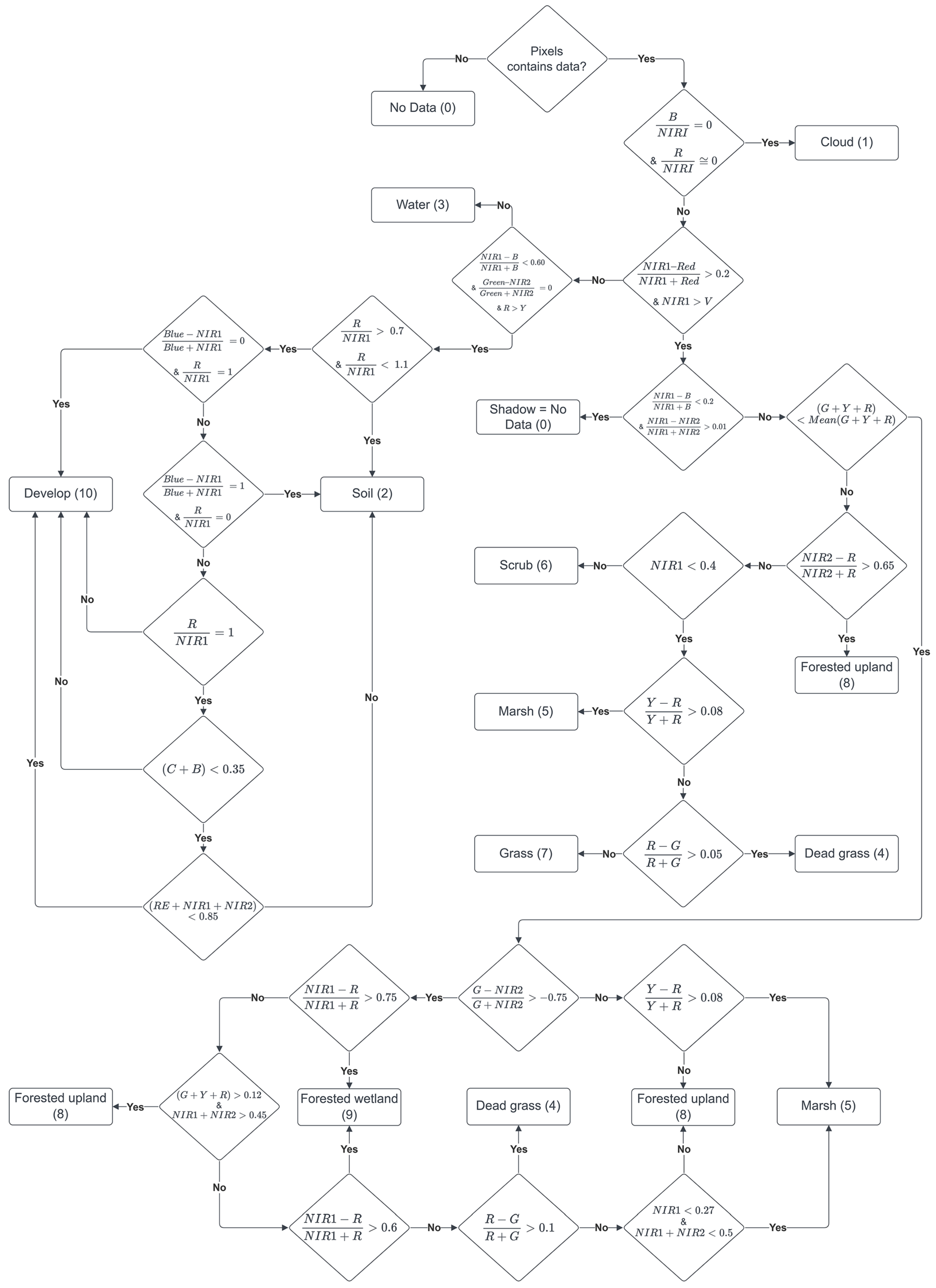
A decision tree developed and tested by McCarthy et al. [11] in West Florida was used for land cover classification, using the spectral bands shown in Table 1. Ten output classes included: clouds, soil, water, dead grass, marsh, scrub, grass, forested upland, forested wetland, and developed land. Pixel values for the classes were from 1 to 10, respectively for each class. Pixels with no data were assigned a value of 0. This included pixels identified as clouds and shadows. The decision nodes used multiple spectral indices and thresholds to make pixel classifications (Figure A1).

We generated a composite land cover map for the whole study area representing January 2012 through December 2015 (inclusive) by stacking classified land cover images and retaining only the maximum classification values pixel-by-pixel (i.e., where pixels from two or more mapped images overlapped, the higher of the classification values was retained). As an example, all classes by definition have a value greater than “clouds” (class value equal to 0), so a “cloud” pixel would always be ignored in favor of a higher-valued class in the final mosaic. This method introduces a potential bias towards higher-valued classes in areas covered by many images compared to areas covered by few images.

The composite map was developed using all useful data between 2012 and 2015. Differences in vegetation at each pixel within this three-year period were considered negligible. We found that differences in vegetation were less than 0.8% per state relative to land cover data between 2013 and 2016 from the NLCD product (

Table A1. Changes (%) in vegetation areas (km²) between the NLCD 2013 and NLCD 2016 products along an elevation band of 0–10 m of different coasts of the southeastern U.S.

Coast	2013 (km2)	2016 (km2)	Change (%)
Texas	18,094	18,235	0.78
Mississippi	1623	1620	−0.16
Louisiana	30,520	30,408	−0.37
Alabama	1027	1026	−0.05
North Florida	14,760	14,730	−0.20
South Florida	16,106	16,063	−0.27

). These changes in vegetation were estimated for a coastal elevation band between 0 and 10 m above mean sea level (see Section 2.6). In specific images, bare land, water, and developed classes were often confused and misclassified in the 2012–2015 mosaic. We recomputed the mosaic for specific areas where misclassifications were observed. In those cases, we prioritized the most probable classes that may occupy that area (e.g., water pixels were priority near inland water bodies and coastal areas; developed pixels were priority in urban areas). We used the 2018 Topologically Integrated Geographic Encoding and Referencing (TIGER) data set from the U.S. Census Bureau to clip the landcover mosaic. We used images covering areas out to the three-mile territorial sea limit along the shoreline. As a consequence, the “water area” estimated from our classification approach is a total measurement including inland, coastal, and three miles of territorial sea. This has no consequence for the study results, which focused on terrestrial land cover classes. The intermediate and final products were included in what we refer to here as the 3D-Wetlands land cover map.

While the classifications used no ground data for training or validation in other areas outside Florida, the composite map from 2012 to 2015 was validated using the USGS NLCD 2016 product, available in GEE. The NLCD is a 30 m resolution Landsat-based product spanning 8 years: 2001, 2004, 2008, 2011, 2013, 2016, 2019, and 2021. It provided rigorously validated land cover data for 20 classes [14]. The NLCD is the best reference available for land cover types along the US Gulf of Mexico coast. We focused validation on total vegetated areas and wetlands only (our “forested wetlands” would be equivalent to “woody wetlands” in the NLCD). We merged some vegetation classes as described in

Table A2. Classes representing the total vegetation from our project 3D-Wetlands and the NLCD product. The classes “forested wetland” (3D-Wetlands) and “woody wetlands” (NLCD) were the only ones similar enough conceptually for a direct comparison.

3D-Wetlands	NLCD
Marsh	Deciduous forest
Scrub	Evergreen forest
Grass	Mixed forest
Forested upland	Shrub/Scrub
Forested wetland	Grassland
	Pasture
	Cultivated crops
	Woody wetlands
	Emergent wetlands

to minimize uncertainties around individual classes. To conduct the validation using NLCD, we generated 1000 random points per state in our vegetated classes located in the 0–10 m topographic elevation band (see Section 2.6). The number of usable points varied due masking of pixels with no data or other causes that led to invalid classes. As result, we identified 835 points in Alabama, 894 in Louisiana, 789 in Mississippi, 848 in Texas, 863 in North Florida, and 641 in South Florida for validation against the NLCD. The locations of those points were sampled over the NLCD 2016 product. 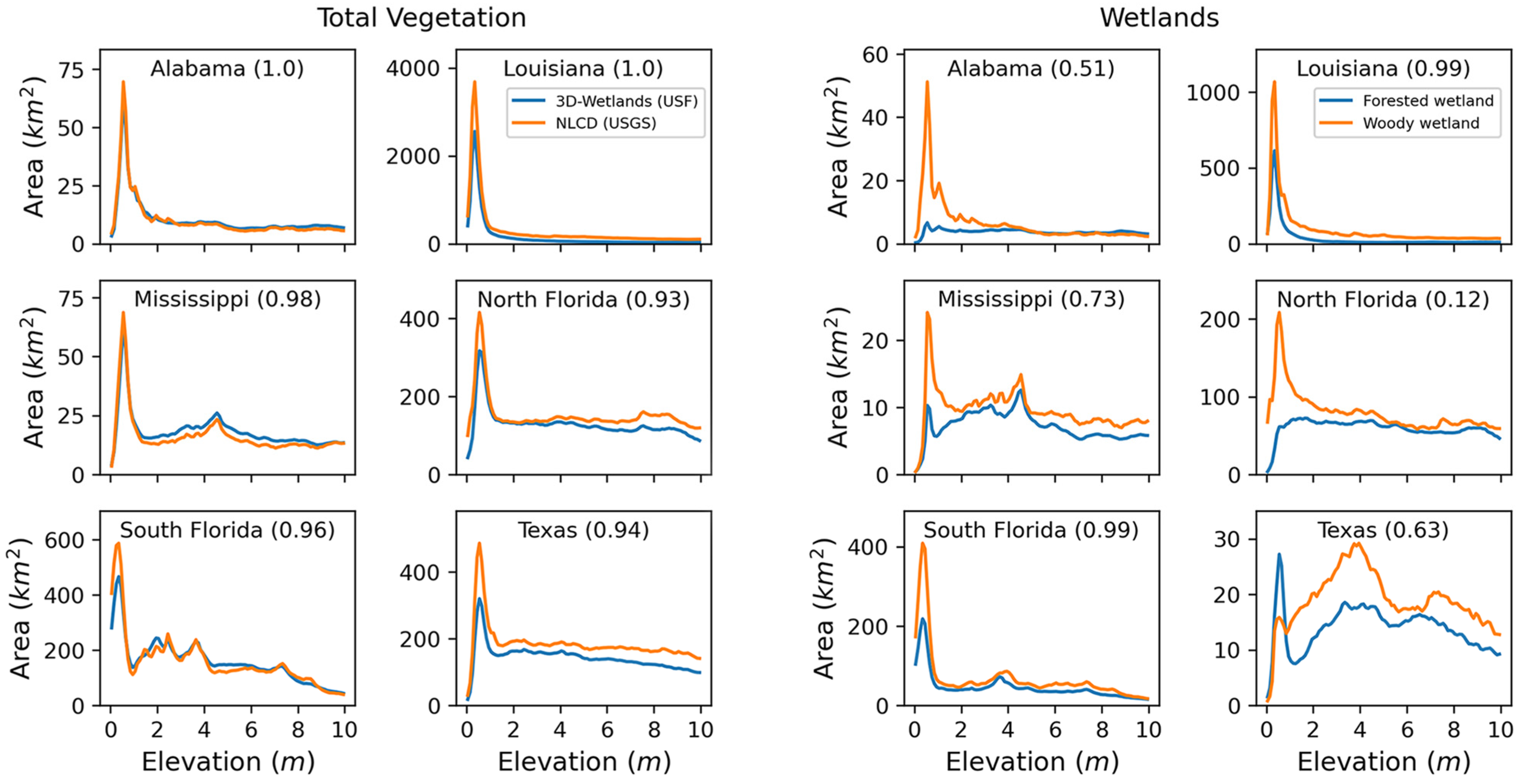We generated error matrices, and the overall accuracy, user’s and producer’s accuracies were estimated [22]. Validation results against the NLCD 2016 product showed that the total vegetation classes were 100% accurate (in overall accuracy, and user’s and producer’s accuracies) in all regions within the 10 m elevation band. The validation for wetlands areas showed variable accuracies (

Table A3. Overall accuracy (OA) and producer’s (PA) and user’s (UA) accuracies of the wetland class validation per state. Accuracies presented in percentages.

State	PA	UA	OA
Alabama	37.1	68.5	47.3
Louisiana	42.9	56.2	73.0
Mississippi	56.5	72.8	60.7
Texas	36.9	37.3	84.8
North Florida	72.4	59.3	61.1
South Florida	49.6	82.7	66.1

). Overall accuracies ranged from 47% to 85%, while the producer’s accuracy from 37% to 72%, and user’s accuracy from 37% to 83%.

2.4. Digital Elevation Model Data

The topographic model to match the landcover classification used 197 Lidar data sets totaling 6.1 TB of point clouds arranged in 193,573 tiles with acquisition dates from 1998 to 2018 (

Table 2. The Lidar data used for the 3D-Wetlands product.

State	UTM Zones	Data Sets	Volume (TB)	Tiles	Years
Texas	14, 15	37	1.69	37,594	2005 to 2018
Louisiana	15, 16	20	0.52	23,657	2002 to 2017
Mississippi and Alabama	16	30	0.72	24,303	1998 to 2018
Florida	16, 17	110	3.17	108,020	2001 to 2018
Total		197	6.10	193,573

). From the original tiles, we generated 281 bare-earth tiles of 40 km by 40 km covering the coastal regions of the 5 U.S. Gulf of Mexico states (

Table A4. The 2 m DEM generated by 40 × 40 km tile for the 3D wetlands product.

State	UTM Zones	Bare-Earth Surface		All-Point Surface
		Tiles	Volume (GB)	Tiles	Volume (GB)
Texas	14	38	56.6	39	58.1
	15	26	38.7	26	38.7
Louisiana	15	51	76.0	58	86.4
	16	14	20.8	14	20.8
Mississippi and Alabama	16	19	28.3	19	28.3
Florida	16	26	38.7	27	40.2
	17	107	159.5	107	159.5
Total		281	418.6	290	432

). The final 2 m by 2 m bare-earth Digital Elevation Model (DEM) products totaled 432 GB. The DEM data set covers approximately 168,135 km² of the study area (Figure 1C).

Lidar data were originally acquired by various entities working to meet different product specifications and using different survey parameters, instruments, software, and procedures. This resulted in varying quality of the Lidar point data. We took a priority weighted averaging approach to join multiple Lidar data sets in areas where there was overlap between surveys to achieve the optimum topographic model to match with WorldView imagery. Thus, the 2 m surfaces were the integrated results of changes in Lidar survey technology, human construction, and natural changes including ground subsidence during the 20-year period sampled. The processing workflow occurred in six phases, as follows:

• Checked metadata of each Lidar survey data set for (1) horizontal and vertical datums, (2) horizontal coordinate system, (3) horizontal unit, (4) elevation unit, (5) geoid used, and (6) nominal point interval.
• Reviewed when and by whom the survey was conducted, and the accuracy provided in the metadata to help in setting the priority of each data set. Data sets with higher accuracy, denser point clouds, and newer acquisition dates had higher priority.
• Converted all Lidar tiles into point clouds having the NAD83 horizontal datum, UTM horizontal coordinate system in meters, NAVD88 vertical datum with vertical coordinate in meters, and the use of Geoid2012b for transformation to NAVD88.
• Generated 2 m pixel elevation surfaces (bare-earth and all-point) on each Lidar tile using an inverse distance weighting algorithm that searches for the 3 nearest points within a 3 m radius of the pixel. Bare-earth and all-points point density per 2 m pixel also were generated for each Lidar tile.
• Mosaicked all elevation surface tiles for each Lidar data set into raster files of 20,000 by 20,000 pixels (40 km by 40 km). Identified data gaps in the raster files using morphological filters and fill gaps by interpolating from neighboring pixels.
• Generated final elevation surfaces by overlapping the mosaicked raster files of these Lidar data sets with priority weighted averaging. In addition, a 10-pixel buffer was used to smooth the surface along edges of Lidar data sets. The final data products were raster files of 20,000 by 20,000 (40 km by 40 km) 2 m pixels covering each UTM zone in each state.

2.5. Sea-Level Trends

Time series of sea level data from 31 tide gauge stations spanning our study area were downloaded from NOAA (https://tidesandcurrents.noaa.gov/sltrends/; accessed on 3 June 2024) (Figure 1D). The seasonal cycle in these data had already been removed by the provider. The coordinates and sea-level trends of each tide gauge station are shown in

Table A5. Tide gauge stations along the US Gulf Coast and Florida. Sea-level rise (SLR) rates and 95% confidence intervals (CI) are also shown.

State	Station Name	Longitude	Latitude	Begin	End	SLR Rate (mm/yr)	95% CI (mm/yr)
Alabama	Dauphin Island	−88.075	30.250	1966	2021	4.25	0.57
Alabama	Mobile State Docks	−88.043	30.708	1980	2021	4.79	1.39
Louisiana	Grand Isle	−89.957	29.263	1947	2021	9.18	0.38
Louisiana	New Canal	−90.113	30.027	1982	2021	6.25	1.11
Mississippi	Bay Waveland	−89.326	30.326	1978	2021	4.68	0.73
Florida (North)	Fernandina Beach	−81.466	30.671	1897	2021	2.20	0.17
Florida (North)	Mayport	−81.428	30.398	1928	2021	2.78	0.25
Florida (North)	Cedar Key	−83.032	29.135	1914	2021	2.27	0.18
Florida (North)	Apalachicola	−84.982	29.727	1967	2021	2.82	0.60
Florida (North)	Panama City	−85.667	30.152	1973	2021	2.91	0.58
Florida (North)	Panama City Beach	−85.879	30.214	1989	2021	4.90	0.95
Florida (North)	Pensacola	−87.211	30.404	1923	2021	2.59	0.23
Florida (South)	Lake Worth Pier	−80.034	26.613	1970	2021	3.82	0.51
Florida (South)	Virginia Key	−80.162	25.731	1931	2021	3.00	0.21
Florida (South)	Vaca Key	−81.106	24.711	1971	2021	3.95	0.42
Florida (South)	Key West	−81.808	24.556	1913	2021	2.52	0.14
Florida (South)	Naples	−81.807	26.132	1965	2021	3.21	0.43
Florida (South)	Fort Myers	−81.871	26.648	1965	2021	3.37	0.44
Florida (South)	St. Petersburg	−82.627	27.761	1947	2021	2.97	0.24
Florida (South)	Clearwater Beach	−82.832	27.978	1973	2021	4.10	0.54
Florida (South)	East Bay	−82.421	27.923	1976	2021	5.68	0.95
Florida (South)	Port Manatee	−82.562	27.638	1976	2021	5.16	0.71
Texas	Sabine Pass	−93.870	29.728	1958	2020	6.16	0.74
Texas	Galveston Pier 21	−94.793	29.310	1904	2021	6.62	0.22
Texas	Galveston Pleasure Pier	−94.789	29.285	1957	2011	6.62	0.69
Texas	Freeport	−95.302	28.943	1972	2020	4.21	0.72
Texas	Rockport	−97.047	28.022	1937	2021	5.94	0.47
Texas	Corpus Christi	−97.217	27.580	1983	2021	5.54	1.00
Texas	Port Mansfield	−97.426	26.558	1963	2021	3.67	0.68
Texas	South Padre Island	−97.168	26.073	1958	2021	4.27	0.54
Texas	Port Isabel	−97.216	26.061	1944	2021	4.25	0.33

.

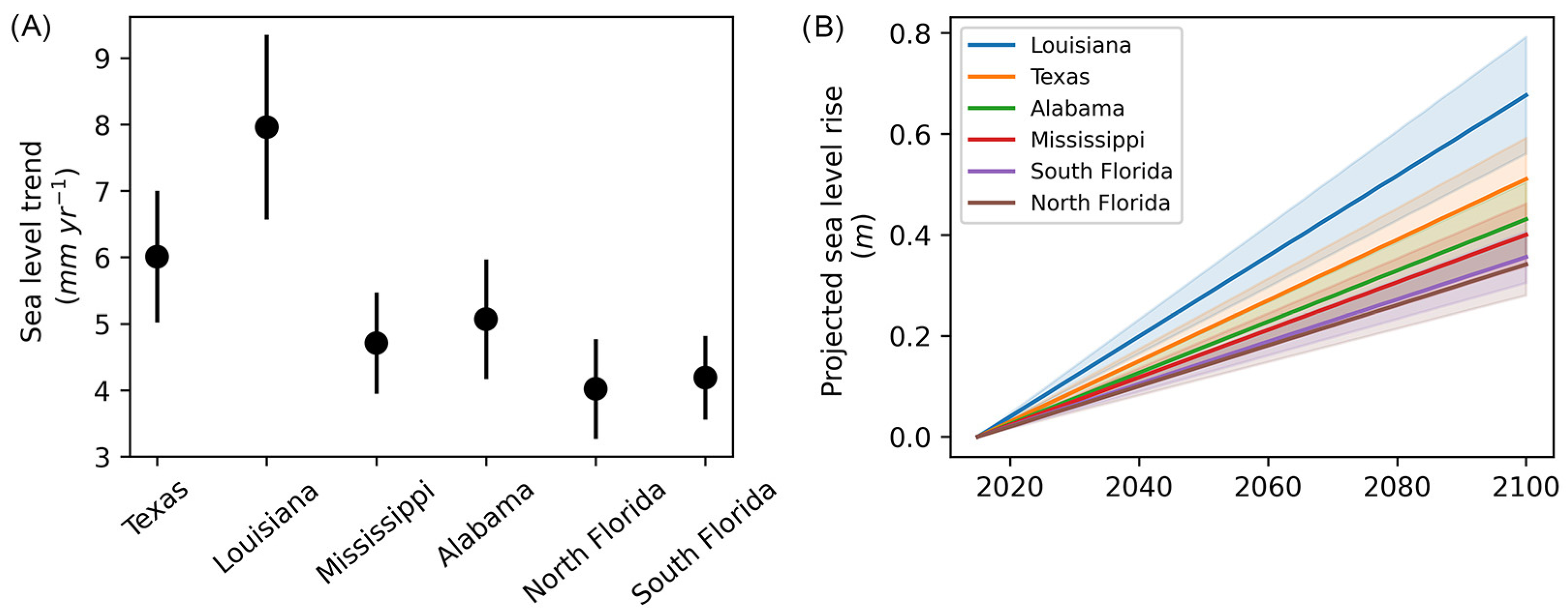
We used data from the period 1983–2021 across the stations to avoid large data gaps that are pervasive in earlier data. To derive trends in sea level, all tide gauge data in each state or in subregions of a state were averaged over a year, and linear sea-level trends (mm yr⁻¹) obtained. The trends were used to project sea level scenarios for the years 2030, 2050, 2070, and 2100, using 2015 as a baseline. SLR was assumed to be linear over the period of the extrapolation; this ignored any possible change in factors that might influence sea level, such as seawater warming rate, hydrological imbalances, land subsidence, and land development rates. Confidence intervals of 90% were calculated as one standard error multiplied by 1.65. The state of Florida was divided into North Florida and South Florida at a latitude of 28.2°N (Figure 1D), to facilitate the analysis and reduce bias due to different sea-level trends (Table A5). Linear trends and confidence intervals were estimated using Scilab v6.1.1.

2.6. Analytical Approach

We used GEE to store 10,245 classified images (2009–2018), create mosaics, and quantify areas. All the classified images and DEMs are publicly available through a GEE App that allows creation of user-defined mosaics, overlay and comparison with topography, aggregation of products at the level of individual counties, and comparing change in land cover over time (https://lizcanosandoval.users.earthengine.app/view/hr-land-cover-gulf-of-mexico; accessed on 3 June 2024).

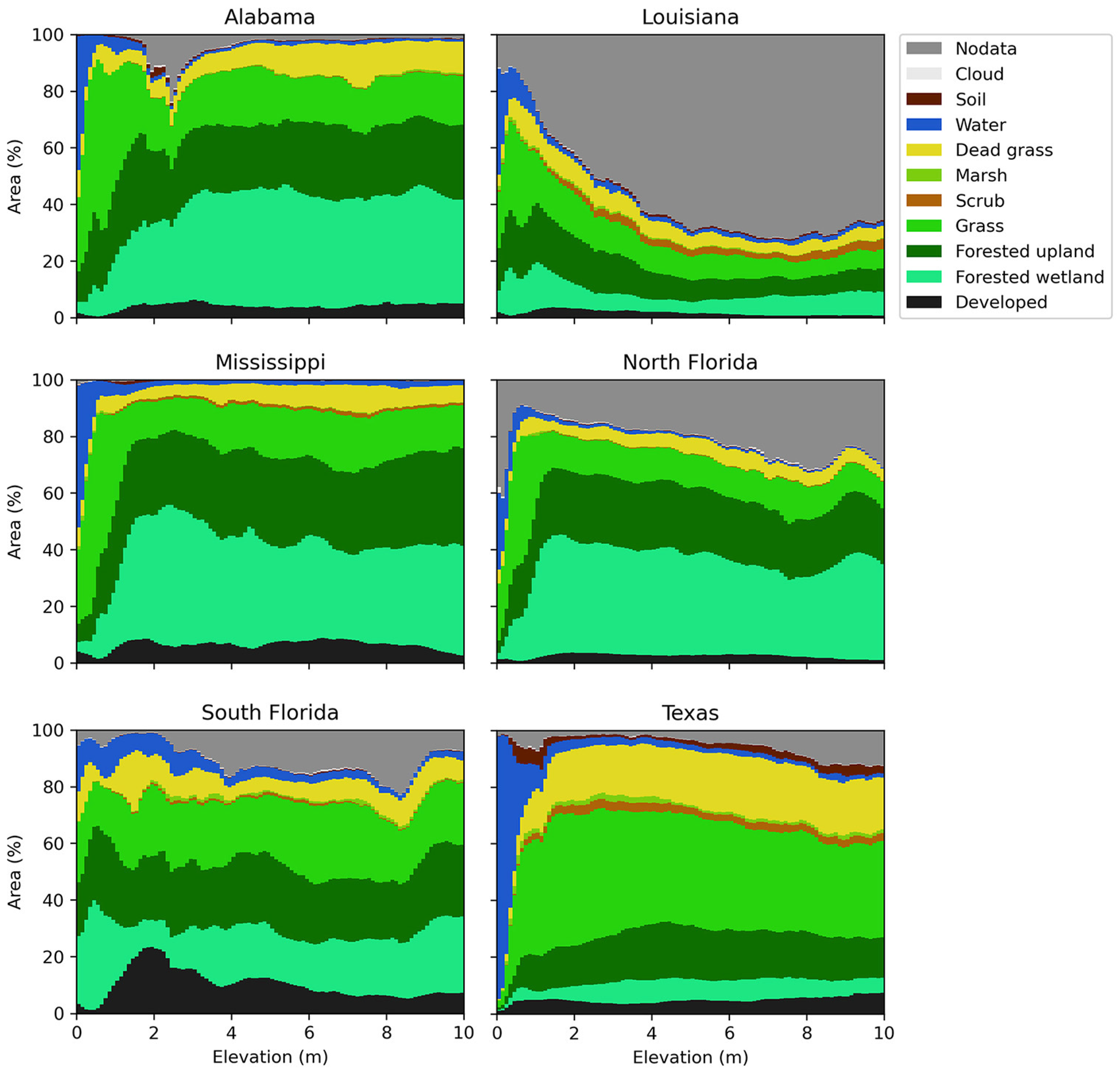
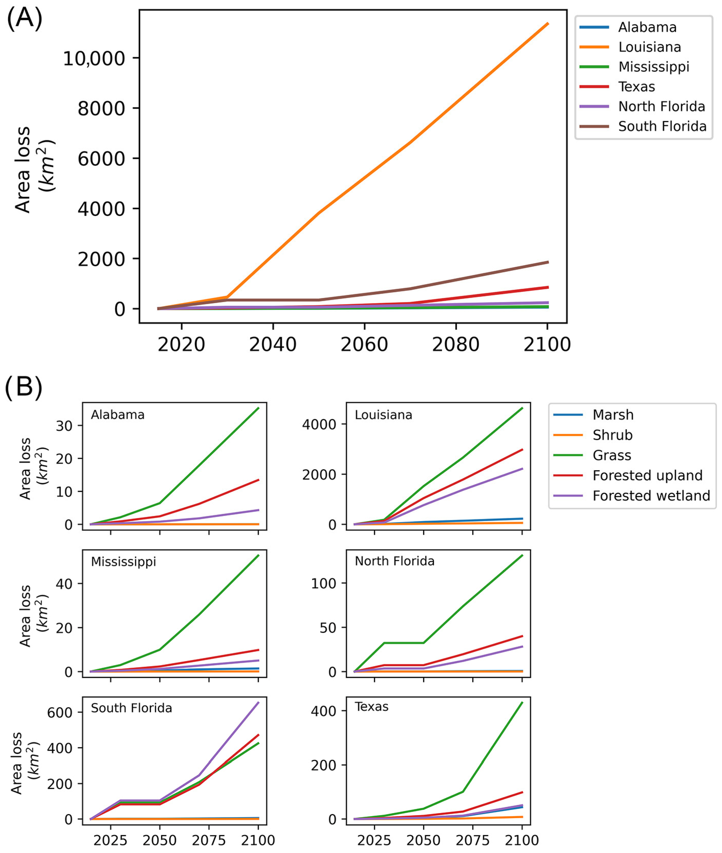
To analyze change in land cover extent in future sea-level rise scenarios, we estimated the surface area covered by each land cover class in each state by multiplying the area of a single pixel (2 m × 2 m) by the number of pixels in a class, as clipped given different future sea level states. The region between the sea and the 10 m coastal elevation is of interest because of potential flood and erosion risk and therefore is a focus for coastal area management. Sea level scenarios projected for 2030, 2050, 2070, and 2100 were used to estimate potential reductions in total surface area for each coastal vegetation class in cumulative elevation bins across the different states, relative to the land cover product for the period 2012–2015.

Sea level projections were made at 0.1 m scale to match the vertical DEM resolution. We focused on relative changes in the total mapped area and the area occupied by five specific vegetation classes: marsh, scrub, grass, forested upland, and forested wetland. We considered marshes and forested wetlands as the principal coastal wetland classes. Total land area estimations excluded pixels classified as no data, cloud, and water. Therefore, any estimates in area extent for any class may be considered conservative.

Comparisons between land cover profiles from our 3D-Wetlands product and the USGS NLCD from 2016 focused on total vegetation and wetlands and they were considered as validation of land cover profiles. Only the NLCD product congruent with the 3D-Wetlands mosaic was used in the comparison. Area estimations were made using the native pixel resolution of each product along the 0–10 m elevation profile at 0.1 m intervals. Pearson’s correlations were made for each comparison between total vegetation and wetlands per state. The area comparisons per elevation ranges can be seen in Figure A2. The correlations of total vegetation between the two products were r > 0.93 in each state, but the wetland areas were more variable being low in North Florida (r = 0.12) and Alabama (r = 0.51), and mid to high in the other states (r > 0.73). Correlation coefficients are shown in Figure A2.

All data were visualized using the Seaborn package in Python and mapped using QGIS v3.18 and the GEE plugin.

3. Results

3.1. Mapped Area

The total area mapped for the period 2012–2015 between the coast and 10 m elevation above sea level in the US Gulf of Mexico was 293,718 km². Of this, we mapped 23,432 km² in Alabama, 52,959 km² in Louisiana, 13,206 km² in Mississippi, 63,602 km² in North Florida, 67,887 km² in South Florida, and 72,632 km² in Texas (this excludes no data and cloudy pixels in the final composite) (Figure 2). Louisiana had the least area covered by satellite imagery (Figure 2 and Figure 3). The total “no data” area in the 10 m elevation coastal band, including cloudy pixels, represented 39.9 km² (3.1%) in Alabama, 12,213 km² (35.2%) in Louisiana, 6.5 km² (0.3%) in Mississippi, 3,873 km² (20.8%) in North Florida, 2224 km² (9.2%) in South Florida, and 1222 km² (5.1%) in Texas. In total, 18.6% of the 10 m elevation band across the entire study region was missing data. We therefore chose to examine abundance of wetland land cover classes relative to overall vegetated land cover classes for each state.

3.2. Vegetation and Wetland Extent within 0–10 m Elevation from the Coast

Within the 10 m coastal vertical profiles of land cover per state composited between 2012 and 2015 (Figure 3), vegetated areas represented between 72.1% and 90.4% of the land area across the different regions (

Table 3. Vegetation and total land area (km²) of the 0–10 m elevation band along the coast of the southeastern United States. Total land area does not include water pixels. Missing data included non-valid pixels and cloud pixels.

Classes	Alabama	Louisiana	Mississippi	North Florida	South Florida	Texas
Marsh	2.9	337.1	5.5	31.1	192.1	355.6
Scrub	2.3	470.9	19.2	45.8	151.2	570.3
Grass	364.8	6889.6	493.5	2879.6	5282.2	8603.5
Forested upland	316.6	5302.0	598.2	4002.6	5589.2	3471.3
Forested wetland	375.6	3758.5	720.0	5950.6	4626.9	1390.6
Total Vegetation	1062.2	16,758.1	1836.3	12,909.8	15,841.6	14,391.3
Total Land	1217.9	19,724.5	2104.5	14,280.2	20,572.8	19,952.1
Missing Data	39.9	12,213.0	6.5	3872.6	2223.7	1221.6

). Coastal wetlands area in relation to the total vegetation area for each state represented 35.6% in Alabama, 24.4% in Louisiana, 39.5% in Mississippi, 46.3% in North Florida, 30.4% in South Florida, and 12.1% in Texas. Total coastal wetland area was 17,746.7 km², of which 60.9% was observed in Florida.

Together, Florida and Louisiana represented 72.5% of the total vegetated areas examined. Forested wetlands were the dominant vegetation type in Alabama, Mississippi, and North Florida. The dominant vegetated classes in Louisiana, Texas, and South Florida were grass and forested upland.

3.3. Mean Sea-Level Trends

The mean sea-level trends computed for the period 1983–2021 show that Louisiana had the fastest SLR rate, with 7.96 mm ± 1.36 mm yr⁻¹. South Florida and North Florida showed the slowest SLR rates at 4.19 mm ± 0.60 mm yr⁻¹ and 4.02 mm ± 0.71 mm yr⁻¹, respectively (Figure 4A). Sea-level projections showed Louisiana will experience an increase of 0.68 m ± 0.12 m by 2100 relative to 2015 (Figure 4B). The overall sea-level increases by 2100 are 0.51 m ± 0.08 m for Texas, 0.43 m ± 0.07 m for Alabama, 0.40 m ± 0.06 m for Mississippi, 0.36 m ± 0.05 m for South Florida, and 0.34 m ± 0.06 m for North Florida. These rates may now be considered conservative as sea-level rise in the region accelerated in the last decade (i.e., 2010–2021), exceeding 10 mm yr⁻¹ in some areas [23].

3.4. Projected Area Loss with SLR

All states show progressive losses in total area with time, and some states will see higher losses due to their topography (Figure 5). The projected losses in total land and vegetation areas due to sea-level rise are largest in Louisiana, due to the highest sea-level rise trend and the large area of low-lying lands. Louisiana is projected to experience a loss of approximately 11,351 km² to be covered by water in 2100. Of this, 88.8% is vegetated area and 11.2% is occupied by other land cover classes (

Table 4. Estimated losses in area (km²) due to sea-level rise by 2100 in the southeastern U.S. Marsh and forested wetland are considered as coastal wetlands in this study. The total land area includes total vegetation and other classes such as soil, dead grass, and developed.

Classes	Alabama	Louisiana	Mississippi	North Florida	South Florida	Texas	Total
Marsh	<0.1	222.9	1.4	0.6	5.4	43.7	273.9
Scrub	<0.1	56.2	<0.1	0.1	0.5	7.7	64.6
Grass	35.2	4623.4	52.7	130.8	424.4	429.1	5695.6
Forested upland	13.4	2971.0	9.8	39.8	470.7	98.5	3603.3
Forested wetland	4.3	2209.1	5.0	28.1	652.7	50.7	2949.8
Vegetation	52.9	10,082.6	68.9	199.4	1553.8	629.7	12,587.2
Land	57.9	11,350.9	78.2	233.7	1846.2	844.7	14,411.7
Water	15.2	2283.7	33.0	115.2	243.5	2051.3	4742.0
No Data	0.1	2019.1	1.2	208.8	82.0	69.8	2381.0

). This is followed by Florida and Texas as these two states have much larger low-lying coastal vegetated areas than Mississippi or Alabama (Figure 5). Alabama and Mississippi are expected to have relatively small coastal land area losses (<80 km²) because they have shorter coastlines and more elevated topography.

In 2100, the area of coastal wetlands (forested wetlands and marshes) at risk of flooding due to SLR is estimated to be at least 2432 km² in Louisiana, 6.4 km² in Mississippi, 94.4 km² in Texas, 28.6 km² in North Florida, and 658 km² in South Florida. The largest gaps in imagery coverage for areas projected to be affected by SLR in 2100 were observed in North Florida (37.4%) and Louisiana (12.9%) (Table 4). Other regions exhibited minor data gaps of <4% (Figure 3). However, even considering these gaps, at least 14,412 km² of land are at risk by 2100 in the southeast U.S. coast, of which 12,587 km² are vegetated areas. Of these areas, 3224 km² comprise wetlands, defined by forested wetlands and marshes.

4. Discussion

The advent of high-speed computing and high-resolution satellite images allows for fast processing of large amounts of data with unprecedented resolution at scale [11]. Still, satellite data often lacks uniform coverage of desired areas over time. Cloud-free coverage of the south and southeast US in the WorldView satellite data catalog is spotty in space and in time. We focused on the 2012 to 2015 period to create a land cover mosaic with only 18.6% data gaps in the 0–10 m elevation band along the coast for this region. The seasonal distribution of images also introduced other artifacts in the land cover mosaic that we did not quantify, including seasonal vegetation changes (phenology), changing water bodies including tides affecting cover in individual images, and changes in remote sensing reflectance simply due to differences in sensor–ground–sun view angles across time. Nevertheless, building composite mosaics of multiple images and retaining the vegetated classes led us to high accuracy assessments from which to project land cover losses due to SLR.

The mosaicking method prioritized vegetation and developed classes. We had misclassifications of the “developed” land class (built environment) because it was challenging to distinguish between developed land and some bare soil areas. These areas are often similar in brightness and confounded the classifier. These misclassifications were corrected manually in post-processing of the land cover products. The final 3D-Wetlands product was consistent with the Landsat-derived NLCD 2016 product. The NLCD 2016 product also has problems with land cover classification accuracies, such as confusion of water with wetlands, forest regrowth with permanent shrub/grasslands, and others, which were addressed in post-processing of the NLCD 2016 [14]. There were some differences between wetland classes of the 3D-Wetlands and NLCD 2016 that were likely due to pixel size differences, diversity in vegetation classes available in the NLCD 2016 product, and undetected misclassification errors, especially in Texas and Louisiana as indicated by the user’s and producer’s accuracies (Table A2). Spatial differences are large considering that one pixel of the NLCD at 30 m can contain 225 pixels of the 3D-Wetlands land cover at 2 m. The validation of the total vegetation showed a confidence of 100% that the 3D-Wetland was indicating vegetation correctly.

Florida and Louisiana are the states with most coastal area between the range of 0 and 10 m elevation, but the higher SLR trends along Louisiana’s coast lead to the largest projected vegetation loss in the region. At least 10,083 km² of Louisiana vegetation will likely be permanently inundated by 2100 relative to 2015. The gaps in our land cover data add some uncertainty by not knowing what land cover classes are represented at specific elevation ranges. Reed et al. [21] modeled three scenarios for Louisiana that corresponded to 0.43 m, 0.63 m, and 0.83 m of SLR between 2015 and 2064. They estimated land losses of 3005 km², 5515 km², and 9986 km², respectively. Our estimates by 2070 (relative to 2015) with 0.44 m of SLR were at least 6620 km² of land loss.

In total, we estimated that more than 12,500 km² of vegetated land will be fully or near permanently covered by water in 2100 along the south and southeast U.S. coast. Different land cover, DEM data, and sea-level rise scenarios used by other studies on the U.S. and global coastal wetlands make it challenging to compare estimated wetland area losses (Table 5). Our study provided wetland extent and measured potential changes due to SLR at the finest available resolutions for the south and southeast coasts of the United States, and the SLR values we found for 2100 (0.3–0.7 m) fall among the mid-range projections (0.5–1.2 m, 90% probability) of a well-established probabilistic SLR model [24].

In this study, we assumed a linear SLR. Yet, global SLR accelerated at a rate of 3.1 mm yr⁻¹ during 1993–2015, while areas along the northeast U.S. coast have shown accelerated rates as large as 6.1 mm yr⁻¹ in the same period [25,26]. Dagendorf et al. [23] estimate even higher rates for the 2010–2021 period (>10 mm yr⁻¹). Some factors influencing SLR (other than deglaciation) at regional scales in the Gulf of Mexico and the U.S. east coasts are thermal expansion associated with the North Atlantic Oscillation and the El Niño-Southern Oscillation [26], river discharges [27], and land subsidence [28,29]. Along with water level changes, other perturbations may occur in coastal areas such as changes in salinity, water quality, and the overall landscape [20,30,31]. Potential vegetation and wetland losses due to SLR have been estimated and modeled under different future scenarios by other authors [18,19,21].

Table 5. Studies of coastal wetland changes due to sea-level rise (SLR) by 2100 in global and U.S. coasts.

Measure	Study Area	Wetland Product	DEM Product	SLR Scenarios by 2100	Reference
Coastal wetland cover and change	Southeast U.S.	3D-Wetlands (2 m)	Lidar (2 m)	0.3–0.7 m	This study
Landward wetland migration	39 estuaries in the Northern Gulf of Mexico coast	NWI (30 m)	Lidar (5, 10, 15 m)	0.5, 1.0, and 1.5 m	Borchert et al. [32]
Coastal wetland change and potential refugia	U.S. Pacific and Atlantic coasts	Wetlands defined by tidal range and elevation data	NOAA Lidar (5 m)	0.5–1.2 m and 0.9–2.4 m	Buchanan et al. [33]
Potential wetland loss and migration areas	U.S. Pacific and Atlantic coasts	C-CAP (30 m)	Not specified	1.5–2.6 m	Osland et al. [20]
Coastal wetland change	Global coast	UNEP WCMC Databases	NASA STRM (90 m)	2.9, 5.0, and 1.1 m	Schuerch et al. [19]
Coastal wetland change	Global coast	GLWD-3 (1 km)	NASA STRM (90 m)	1 m	Blankespoor et al. [18]

Table 5. Studies of coastal wetland changes due to sea-level rise (SLR) by 2100 in global and U.S. coasts.

Measure	Study Area	Wetland Product	DEM Product	SLR Scenarios by 2100	Reference
Coastal wetland cover and change	Southeast U.S.	3D-Wetlands (2 m)	Lidar (2 m)	0.3–0.7 m	This study
Landward wetland migration	39 estuaries in the Northern Gulf of Mexico coast	NWI (30 m)	Lidar (5, 10, 15 m)	0.5, 1.0, and 1.5 m	Borchert et al. [32]
Coastal wetland change and potential refugia	U.S. Pacific and Atlantic coasts	Wetlands defined by tidal range and elevation data	NOAA Lidar (5 m)	0.5–1.2 m and 0.9–2.4 m	Buchanan et al. [33]
Potential wetland loss and migration areas	U.S. Pacific and Atlantic coasts	C-CAP (30 m)	Not specified	1.5–2.6 m	Osland et al. [20]
Coastal wetland change	Global coast	UNEP WCMC Databases	NASA STRM (90 m)	2.9, 5.0, and 1.1 m	Schuerch et al. [19]
Coastal wetland change	Global coast	GLWD-3 (1 km)	NASA STRM (90 m)	1 m	Blankespoor et al. [18]

Resilience of wetlands to SLR and their capacity to migrate will depend on availability of accommodation space, which is influenced by sediment deposition rates, coastal human population, and infrastructures [19,20,32,33,34,35]. This might cause losses in aboveground carbon in the future due to potential transitions from forests to marshes [36]. However, recent findings on the organic production (vertical accretion) of coastal wetlands suggests that these ecosystems might keep the pace with SLR. Morris and Sundberg [37] found in monitoring sites at North Inlet estuary, South Carolina that marshes had higher rates of positive elevation (4.7 mm yr⁻¹) than the local rate of SLR (3.4 mm yr⁻¹) due to organic production, suggesting a possible stability of the ecosystem for more than a century. Similar findings by Weston et al. [38] along the US East coast suggest accelerated marsh accretion in response to SLR. Tidal regimes also play a role in wetland accretion rates. Belliard et al. [39] found that several global coastal wetland sites with semi-diurnal tides show positive elevation changes relative to local SLR, in contrast to other tidal regimes such as diurnal and mixed-diurnal, where elevation deficits were observed.

If wetland refugia are conserved (with no human development) under optimistic scenarios (high positive surface elevation change rate of 8 to >10 mm yr⁻¹ and low greenhouse gas emissions), wetlands may increase by 25% in the United States, except for Louisiana [33]. Conservation and restoration strategies will be costly. The state of Louisiana already invested nearly USD 300 million in wetland restoration between 2012 and 2017 [40], and planned diversions of the Mississippi River are caught in contentious political discussions that risk accelerated land losses if not resolved. Overall, potential wetland drowning may represent losses of upwards of USD 732 billion in annual ecosystem services by 2100 in the United States [33].

5. Conclusions

The 3D-Wetlands land cover product demonstrated high accuracy in indicating vegetation, highlighting its reliability for further analysis in wetland areas. High-resolution land cover and topography products will enable more accurate estimations and potential studies on coastal wetlands. Regional differences in vegetation losses due to SLR are more critical in lowland areas such as Louisiana, which is expected to suffer the largest losses in vegetation area by 2100, including a large portion of coastal wetlands across the Northern Gulf of Mexico coast. This vulnerability underscores the importance of understanding coastal wetland extent and distribution for effective management, conservation, and planning.