A Land-Corrected ASCAT Coastal Wind Product

Abstract

A new ASCAT coastal wind product based on a 12.5 km grid size is presented. The new product contains winds up to the coast line and is identical to the current operational coastal product over the open ocean. It is based on the assumption that within a wind vector cell land and sea have constant radar cross section. With an accurate land fraction calculated from ASCAT’s spatial response function and a detailed land mask, the land correction can be obtained with a simple linear regression. The coastal winds stretch all the way to the coast, filling the coastal gap in the operational coastal ASCAT product, resulting in three times more winds within a distance of 20 km from the coast. The Quality Control (QC), based on the regression error and the regression bias error, reduces this abundance somewhat. A comparison of wind speed pdfs with those from NWP forecasts shows that the influence of land in the land-corrected scatterometer product appears more reasonable and starts not as far offshore as that in the NWP forecasts. The VRMS difference with moored buoys increases slightly from about 2.4 m/s at 20 km or more from the coast to 4.2 m/s at less than 5 km, where coastal wind effects clearly contribute to the latter difference. While the QC based on the regression bias error flags many WVCs that compare well with buoys, the land-corrected coastal product with more abundant coastal winds appears useful for nowcasting and other coastal wind applications.

1. Introduction

Accurate wind measurements in the coastal region are of utmost importance for all kinds of offshore activities, and in particular for nowcasting applications, related, e.g., to transport, energy, and tourism. Wind scatterometers, like QuikScat or ASCAT, have been well proven to give accurate wind measurements over the ocean [1], which are, for example, used for assimilation in NWP models, nowcasting, climate data records, and the forcing of ocean models for ocean circulation, waves, or tides. Scatterometers are rather sensitive to land contamination, and therefore their use is limited to distances more than about 20 km from the coast [2].

Long et al. [3] solved this by deconvoluting the measured normalized radar cross sections, NRCS or ${\sigma }^0$, with the spatial response function (SRF) of the scatterometer to a fine grid of the order of a few kilometers. This not only yields wind fields at a very high spatial resolution but also winds that are close to the coast line. The method has been applied to QuikScat and ASCAT [4]. A disadvantage of this method is that it is computationally too intensive for near-real-time applications.

Another approach was followed for a global QuikScat processing, where global coastal land ${\sigma }^0$ values were estimated, which were subsequently used to correct for land contamination near the coast [5], using a computed Land Contribution Ratio (LCR) for each coastal ${\sigma }^0$ measurement. The land ${\sigma }^0$ value is typically an order of magnitude higher than ocean values and the land ${\sigma }^0$ variability is used for soil moisture detection.

In this paper, yet another approach is followed, starting from an improved ASCAT full-resolution L1B radar cross section product. Recently, EUMETSAT developed a new land fraction for this product, based on a parameterization of the ASCAT spatial response function [6] and the high-resolution Global Self-consistent Hierarchical High-resolution Geography (GSHHG) coast line map [7]. This new land fraction became operational over the course of 2022, while to prepare for the wind application elaborated here, EUMETSAT processed all ASCAT-B data from 2017 with the new land fraction.

The land correction algorithm presented here is based on the assumption that within a coastal wind vector cell (WVC), the radar cross sections of land and sea are constant for each view (i.e., from the fore, mid, or aft beam). The radar cross section of the sea is estimated from a regression analysis of the measured ${\sigma }^0$ values against the land fraction. The analysis is carried out for each beam at each coastal WVC using all L1B footprints contributing to that WVC view. A critical parameter is the maximum land fraction allowed in the regression analysis. Low values add only a few coastal WVCs, while high values may yield erroneous winds. The optimal value, determined from visual inspection, lies around 0.5. For WVCs over the open ocean, where all the L1B footprints have a land fraction below 0.02, standard processing is applied. More detailed information can be found in the validation report [8]. The land correction algorithm adds only a few seconds to the processing time and is operationally applied at KNMI from 22 November 2022 onwards on behalf of the Ocean and Sea Ice Satellite Application Facility (OSI SAF).

This paper is organized as follows. In Section 2, the land correction algorithm is presented in detail. The land-corrected product is compared to NWP forecasts in Section 3 and to moored buoy measurements in Section 4. This paper ends with the conclusions and some recommendations for future work in Section 5.

2. Land Correction Algorithm

Scatterometer wind data are given on a regular grid of wind vector cells. ASCAT wind processing exploits a triplet of radar cross section values from the fore, mid, and aft beams, respectively. Each cross section in the triplet is an unweighted average of all full-resolution measurements that fall within a specified distance from the center of the WVC. For a grid size of 12.5 km, the distance is 15 km at most, and the number of full-resolution measurements contributing to a WVC varies from about 25 for the mid beam at low incidence angles to about 45 for the fore and aft beams at high incidence. Without land correction, a full-resolution measurement is rejected if its land fraction is more than 0.02 based on a coarse land mask [2]. The land correction algorithm attempts to correct and use these coastal measurements.

Suppose now that in the coastal region for each individual WVC and for each beam separately the radar cross section of the contributing full-resolution measurements (in linear units) depends linearly on the land fraction $f$ as

$${\sigma }^0=af+b$$

(1)

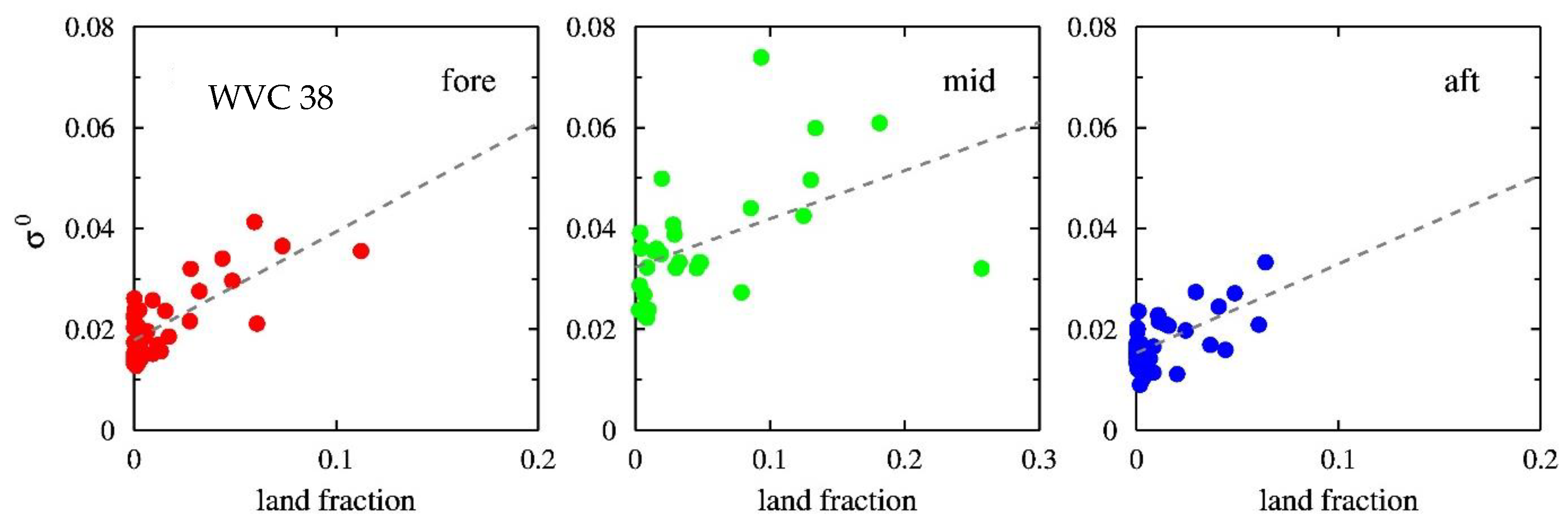
For zero land fraction, this yields the radar cross section of the sea, ${\sigma }_{sea}^0=b$; for a unit land fraction, ${\sigma }_{land}^0=a+b$. Figure 1 shows a real example (row 106 and WVC 38 of the first ASCAT-B file of 2017). The dots represent the radar cross section values for the fore, mid, and aft beams, respectively, and the dashed line is the regression line.

The coefficients $a$ and $b$ can be obtained by linear regression as

$$a=\frac{C_{f\sigma }}{C_{ff}}$$

(2)

$$b=M_{\sigma }-a{M}_f$$

(3)

where $M_x$ is the first moment of quantity $x$ and $M_{xy}$ are second moments, with $x,y=\sigma ,f$. Further, $C_{xy}=M_{xy}-M_x{M}_y$. Once the regression coefficients are known, each full-resolution radar cross section ${\sigma }^0$ can be corrected as

$${\sigma }_{sea}^0={\sigma }^0-af$$

(4)

The ${\sigma }_{sea}^0$ values for each WVC are averaged per beam to obtain the triplet of mean radar cross sections used for wind retrieval.

The regression analysis also yields further information that may be useful for quality control. The mean square error (MSE) of the regression, ${\sigma }_e,$ is given by

$${\sigma }_e^2=\frac{n}{n-2}\left(C_{\sigma \sigma }-2a{C}_{f\sigma }+a^2{C}_{ff}\right)$$

(5)

with $n$ the number of $\left(f,\sigma \right)$ pairs in the regression. Assuming Gaussian errors (a rather optimistic assumption in practice), the standard deviations in the regression coefficients $a$ and $b$, denoted as ${\sigma }_a$ and ${\sigma }_b$, respectively, read

$${\sigma }_a^2=\frac{{\sigma }_e^2}{n{C}_{ff}}$$

(6)

$${\sigma }_b^2={\sigma }_a^2{M}_{ff}$$

(7)

Only ${\sigma }_b^2$ showed any skill as a quality indicator, as shown in Section 4.2. The use of ${\sigma }_e^2$ is described below.

A crucial parameter is the maximum land fraction, $f_{max}$, which is allowed in the regression analysis. Increasing $f_{max}$ leads to more WVCs processed, but also to more uncertainty in the retrieved winds. Visual inspection of results yielded a value of 0.5 as the best compromise between data quantity and data quality.

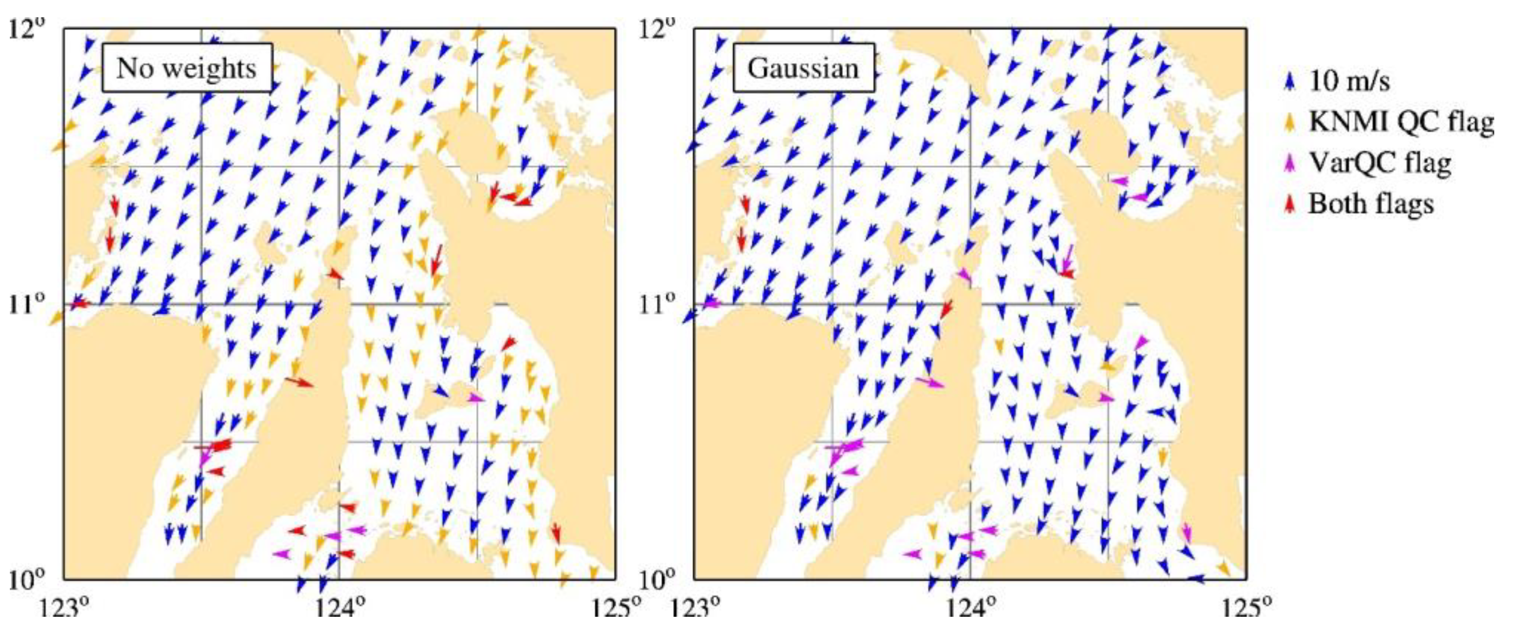
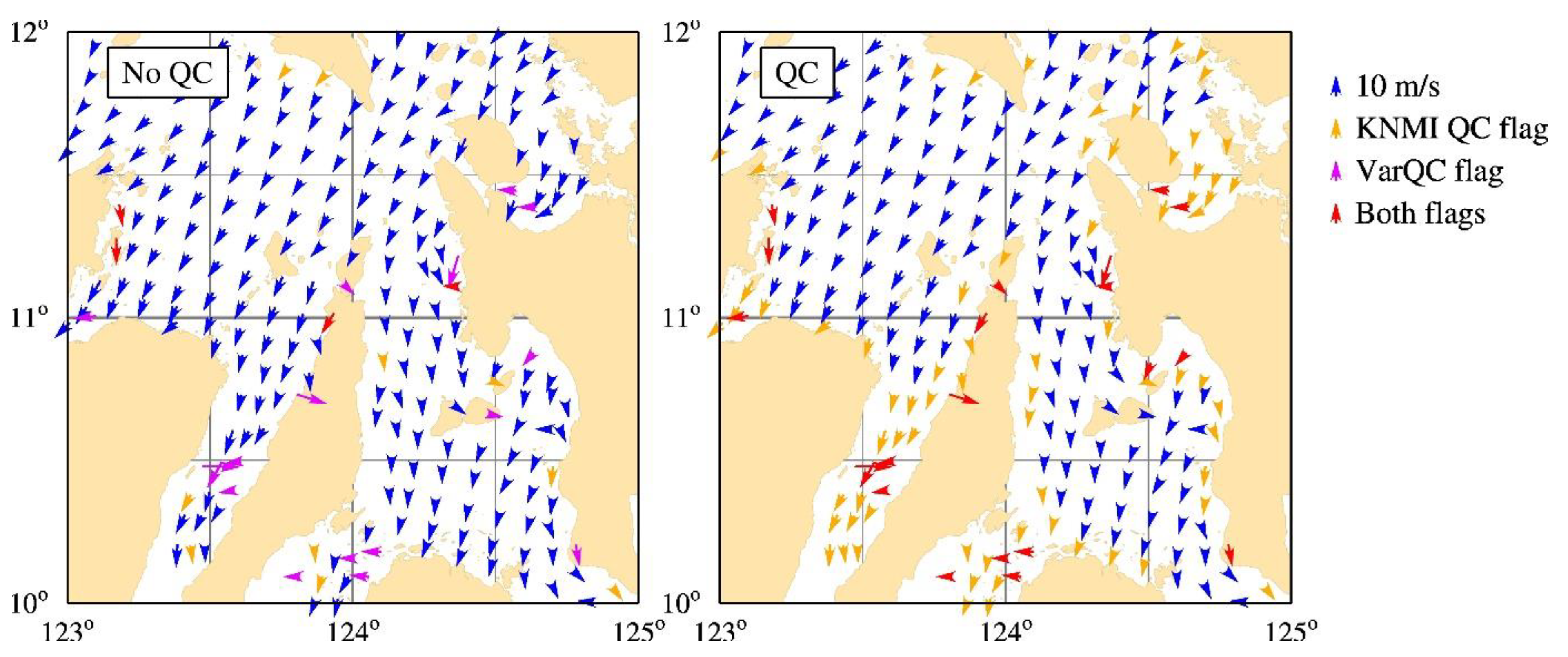
Figure 2 shows two coastal wind fields over the Philippines recorded on 1 January 2017. The left one is processed without any quality control, and many reasonable-looking wind vectors very close to the coast have the KNMI QC flag raised (orange arrows). Further analysis showed that this is mainly caused by the noise estimate $K_p$ exceeding its threshold of 10.0%. This may be due to increased wind variability near the coast and/or variations in ${\sigma }^0$ over land. Whatever the cause, $K_p$ can be reduced by eliminating the effect of full-resolution ${\sigma }^0$ values too far from the regression line using the regression error ${\sigma }_e^2$ (5). The distance to the regression line, $∆$, reads as

$$∆={\sigma }^0-af-b$$

(8)

After some experimentation, good results were obtained by adding Gaussian weights to the full-resolution ${\sigma }^0$ values used to calculate $K_p$ in WVCs where the land correction is applied. The weights read as

$$w=\exp \left(-{\left[\frac{∆}{{\sigma }_e}\right]}^2\right)$$

(9)

The result is shown in the right-hand panel of Figure 2. Now, the KNMI QC flag setting frequency is strongly reduced along the coast.

3. Validation and NWP Comparison

First, we present the gain in the number of coastal WVCs for the land-corrected coastal product with respect to the operational product in

Table 1. Global number of valid coastal WVCs as a function of coastal distance bins in millions (M) for January 2017.

Bin [km]	0–10	10–20	20–30	30–40	40–50	0–30
N Ops. [M]	0.2	0.7	1.2	0.9	0.8	2.1
N Coastal [M]	1.5	1.2	0.9	0.9	0.8	3.6

. The data in Table 1 are for one month (January 2017). In the area within 30 km of land, about 70% more WVCs are processed into valid winds. Further away from land, the same number of WVCs is processed for the land-corrected and operational products. Note that all WVCs are evaluated on a regular swath grid, but the eventual WVC location is the geographical mean of the contributing (corrected) ${\sigma }^0$ measurements, where the geographical mean location remains generally very close to the WVC center location. As a result, close to the coast, the number of processed WVCs increases somewhat with respect to the about 800,000 winds per 10 km bin further away from the coast.

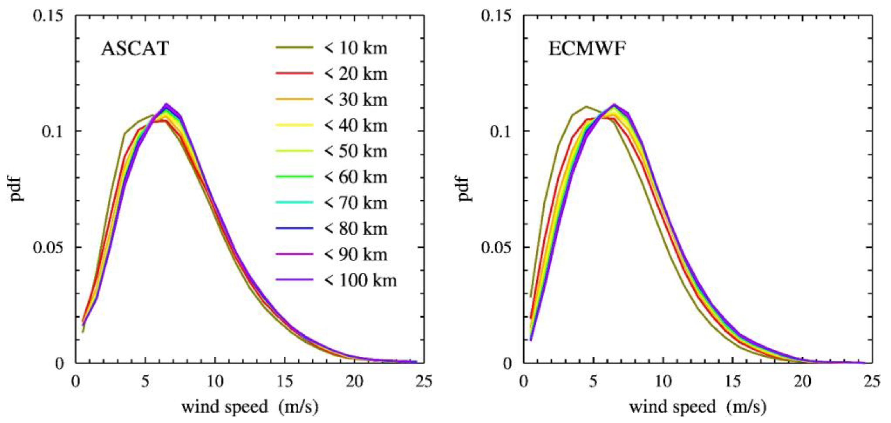
As for the operational ASCAT wind products, a forecast of the ECMWF model with a lead time of at least 3 h is collocated with each WVC. Figure 3 shows the wind speed pdfs for the land-corrected product (left-hand panel) and for the collocated ECMWF forecasts (right-hand panel) as a function of the distance to the coast in bins of 10 km, indicated by the colors of the curves. The pdfs were made for January 2017.

Figure 3 shows that the peaks of the pdfs shift towards lower wind speeds as the distance to the coast decreases. For the land-corrected product, the shift starts at distances below 20 km, but for high wind speeds, the pdf remains the same. Note that land backscatter is much stronger than sea backscatter and therefore land contamination particularly enlarges the lowest winds. No signs of remaining land contamination appear in the corrected product. Further note that the ECMWF pdfs, however, start to shift at distances of about 40 km, and the whole pdf is shifted towards lower wind speed. It is known that the ECMWF model spreads the influence of the land at too large distances from the coast, making it less suitable for further quantitative comparison. Nevertheless, the behavior of the pdfs of the land-corrected wind speed looks realistic.

Further checks and balances for on-shore, off-shore and parallel winds to the coast, including ${\sigma }^0$ pdfs, inversion residuals, and quality control indicators as a function of distance (and direction) to the coast are provided in [8], confirming the above summary conclusions.

4. Buoy Comparison

4.1. Buoy Data

The buoy dataset was collected from three sources:

• The Copernicus Marine Service In Situ Thematic Assembly Centre (IS TAC), www.marineinsitu.eu (accessed on 1 May 2024), in NetCDF format;
• The Meteorological Archival and Retrieval System (MARS) from ECMWF in BUFR format;
• The National Data Buoy Centre (NDBC) from NOAA, www.ndbc.noaa.gov (accessed on 1 May 2024), in ASCII.

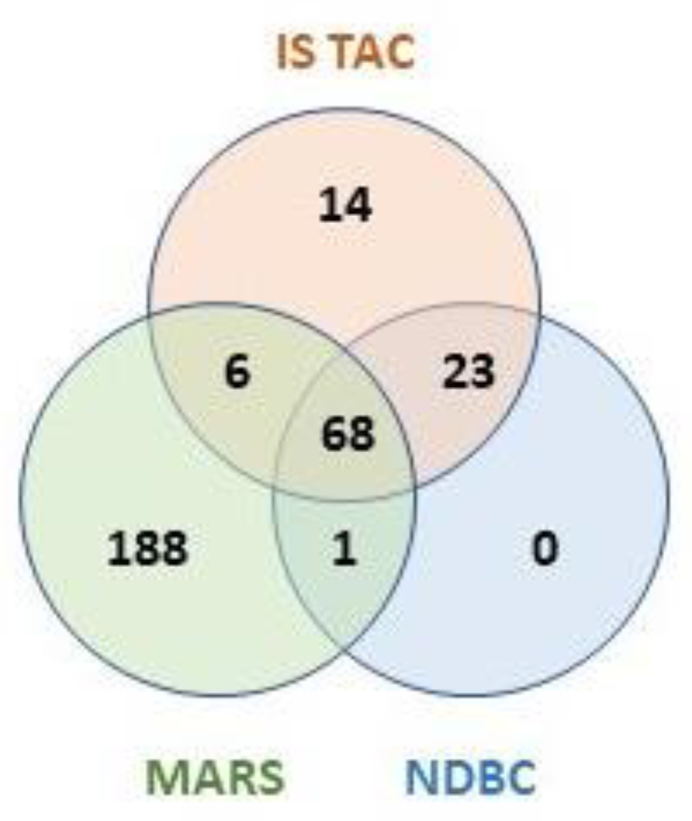
The IS TAC and NDBC datasets are freely available online. The MARS data are available for ECMWF members, but researchers from other institutes can apply for a license for non-commercial use. Due to the large number of buoys in the MARS dataset (see Figure 4), we include this dataset in the analysis.

The buoy winds were converted to 10 m stress-equivalent winds using the COARE-3.6 algorithm [9,10]. The availability of metadata such as anemometer height and temperature sensor heights strongly limits the number of usable buoys. For 300 buoys, metadata were available in the data themselves or in metadata files made available by the data supplier, and the transformation to stress-equivalent winds could be carried out. In case the surface pressure was missing, it has been interpolated from ECMWF analyses and forecasts. This is legitimate, as the COARE algorithm depends only very weakly on surface pressure. The three buoy datasets are partly overlapping, as shown in Figure 4, though the number of measurements per buoy may differ. In case of overlapping data for the same buoy, the set with the most data values was chosen.

Note that the NDBC buoys are all present in the IS TAC or the MARS dataset, but in a number of cases, the NDBC buoys have the largest number of data points and are to be preferred.

4.2. Quality Control and Comparison

Table 2. VRMS difference between buoy winds and land-corrected ASCAT winds and the number of points from which the VRMS is calculated as a function of the buoy distance to the coast in 5 km bins for the land-corrected product without and with quality control.

Distance to Coast (km)	No QC		QC
	VRMS (ms−1)	Nr of Points	VRMS (ms−1)	Nr of Points
0–5	7.2	1787	4.2	226
5–10	4.8	3110	3.1	1477
10–15	3.3	4553	3.0	3122
15–20	3.2	2676	3.0	2187
20–25	2.4	1953	2.4	1862
25–30	2.2	1563	2.2	1461
30–35	2.7	4233	2.7	4136
35–40	2.1	1427	2.1	1386

gives the vector root-mean-square (VRMS) difference between the buoy winds and the land-corrected winds (second column) and the number of points from which the VRMS is calculated (third column) as a function of the buoy distance to the coast in 5 km bins (first column) for all 2017. WVCs that have the KNMI QC and/or the VarQC flag set are excluded from the comparison.

Without any further quality control, the VRMS differences increase from an open ocean value of about 2.4 m/s to 7.2 m/s for buoys 5 km or less from the coast (second column in Table 2). This large number is caused by some buoys at unfavorable positions: one in a fjord in Alaska and some buoys in the Great Lakes. One could exclude these buoys, but that would give only a cosmetic improvement in the comparison results, as it says nothing about the quality of the land-corrected wind at other coastal locations.

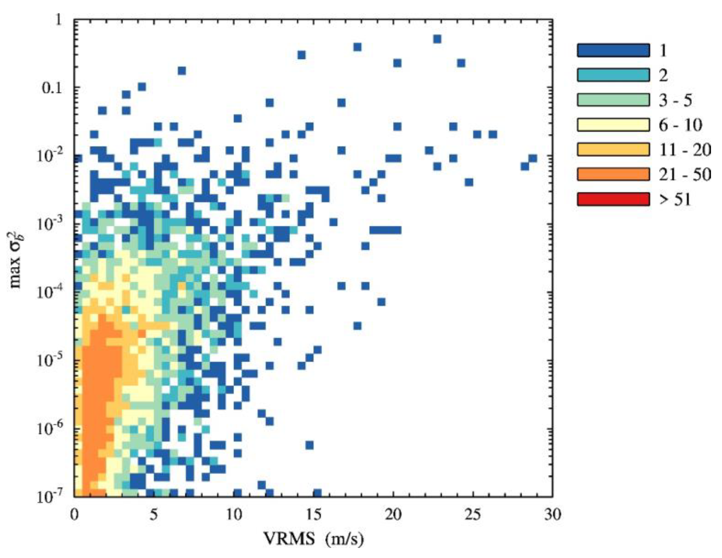
After some experimentation, the regression bias error variance ${\sigma }_b^2$ in Equation (7) showed some skill in detecting outliers, as can be inferred from Figure 5. This figure shows the maximum value of ${\sigma }_b^2$ over the fore, mid, and aft beams against the VRMS difference of buoy winds and land-corrected winds. The y-axis in Figure 5 is logarithmic, as the regression bias error has a considerable range.

Imposing a threshold value of 0.000015 (1.5 × 10⁻⁵) on ${\sigma }_b^2$ and setting the KNMI QC flag for WVCs in which this threshold is exceeded reduces the VRMS near the coast considerably, as can be seen from the fourth column in Table 2. However, the last column shows that the number of points is also reduced considerably. Figure 5 shows that at this value also a large number of WVCs that compare well with buoys is flagged. The effect of this can be seen in Figure 6, which shows the same scene as Figure 2. The left-hand panel of Figure 6 is without threshold on ${\sigma }_b^2$ and is identical to the right-hand panel of Figure 2. The right-hand panel of Figure 6 is with the threshold of 0.000015 on ${\sigma }_b^2$, where WVCs for which the threshold is exceeded have the KNMI QC flag raised (orange arrows).

Figure 6 shows that the quality control based on the regression bias error is not restrictive enough, though the land-corrected product can very well be used for nowcasting applications.

5. Conclusions and Outlook

A new ASCAT coastal land-corrected product with a 12.5 km grid size is presented. The land correction is obtained from linear regression of the full-resolution radar cross section against the land fraction, assuming that the radar cross sections of land and sea within a wind vector cell are constant. The land fraction is calculated from parametrized spatial response functions and a high-resolution coast line map. The full-resolution radar cross section values within a wind vector cell are averaged with Gaussian weights, the width of these dependent on the regression error. A threshold on the regression bias error is imposed to reject WVCs, whose wind differs too much from collocated buoy winds. The land-corrected product exhibits a more realistic behavior near the coast than the ECMWF forecasts: the influence of land becomes visible in the wind speed pdfs at smaller distances to the coast and affects mainly small to moderate winds. Comparison with buoys shows that the VRMS of the difference between buoy winds and land-corrected winds increases from about 2.4 m/s for buoys 20 km or more from the coast to 4.2 m/s for buoys less than 5 km from the coast. Though the quality control based on the regression bias error flags too many wind vector cells that compare well with buoys, the land-corrected product is very well usable for nowcasting and other coastal wind applications. The land correction is applied operationally for the OSI SAF ASCAT coastal wind products from 22 November 2022 onwards.

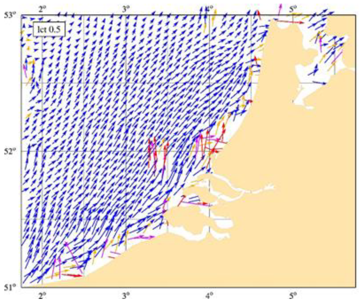
The authors suggest further work using high-spatial-resolution SAR winds for large structures (harbors, etc.), breaking waves on shore, Radio Frequency Interference, lakes, (tidal) currents, etc. Investigating collocated ASCAT and SAR images will be useful to better understand these effects in future work. Figure 7 shows an ASCAT high-resolution wind product, processed with the land correction presented in this paper, showing the prospects at this resolution. Finally, the land correction method by regression is also being applied for pencil-beam scatterometers, following the successful application for ASCAT [11].

References

1. Vogelzang, J.; Stoffelen, A. On the Accuracy and Consistency of Quintuple Collocation Analysis of In Situ, Scatterometer, and NWP Winds. Remote Sens. 2022, 14, 4552. [Google Scholar] [CrossRef]
2. Verhoef, A.; Portabella, M.; Stoffelen, A. High-resolution ASCAT scatterometer winds near the coast. IEEE Trans. Geosci. Rem. Sens. 2012, 50, 2481–2487. [Google Scholar] [CrossRef]
3. Long, D.G.; Luke, B.J.; Plant, W. Ultra high resolution wind retrieval for SeaWinds. In Proceedings of the IGARSS 2003—IEEE International Geoscience and Remote Sensing Symposium, Toulouse, France, 21–25 July 2003; pp. 1264–1266. [Google Scholar] [CrossRef]
4. Hutchings, N.; Kilpatrick, T.; Long, D.G. Ultrahigh Resolution Scatterometer Winds near Hawaii. Remote Sens. 2020, 12, 564. [Google Scholar] [CrossRef]
5. Fore, A.G.; Stiles, B.W.; Strub, P.T.; West, R.D. QuikSCAT Climatological Data Record: Land Contamination Flagging and Correction. Remote Sens. 2022, 14, 2487. [Google Scholar] [CrossRef]
6. Lindsley, R.D.; Anderson, C.; Figa-Saldaña, J.; Long, D.G. A parameterized ASCAT measurement spatial response function. IEEE Trans. Geosci. Remote Sens. 2016, 54, 4570–4579. [Google Scholar] [CrossRef]
7. Wessel, P.; Smith, W.H.F. A Global Self-consistent, Hierarchical, High-resolution Shoreline Database. J. Geophys. Res. 1996, 101, 8741–8743. [Google Scholar] [CrossRef]
8. Vogelzang, J.; Stoffelen, A. ASCAT Land Correction. Report SAF/OSI/CDOP3/KNMI/TEC/TN/384. Available online: https://scatterometer.knmi.nl/publications/pdf/ASCAT_land_correction_v1.0.pdf (accessed on 14 April 2024).
9. Fairall, C.W.; Bradley, E.F.; Hare, J.E.; Grachev, A.A.; Edson, J.B. Bulk Parameterization of Air-Sea Fluxes: Updates and Verification for the COARE Algorithm. J. Clim. 2003, 16, 571–591. [Google Scholar] [CrossRef]
10. Cronin, M.F.; Fairall, C.W.; McPhaden, M.J. An assessment of buoy derived and numerical weather prediction surface heat fluxes in the tropical Pacific. J. Geophys. Res. 2006, 111, C06038. [Google Scholar] [CrossRef]
11. Grieco, G.; Portabella, M.; Stoffelen, A.; Verhoef, A.; Vogelzang, J.; Zanchetta, A.; Zecchetto, S. Coastal wind retrievals from corrected Quikscat normalized radar cross sections. Remote Sens. Environ. 2024, 308, 114179. [Google Scholar] [CrossRef]
Figure 1. Example of land correction by regression for row 106 and WVC 38 of the first ASCAT-B file of 2017. The dots represent the radar cross section values for the fore, mid, and aft beams from left to right and the dashed line is the regression line used to correct the colored dots for each associated land fraction.
Remotesensing 16 02053 g001
Figure 2. Land-corrected wind fields over the Philippines on 1 January 2017 without weighted full-resolution radar cross sections (left-hand panel) and with Gaussian weights (right-hand panel).
Remotesensing 16 02053 g002
Figure 3. Wind speed pdfs as a function of the distance to the coast in 10 km bins for the land-corrected ASCAT product (left-hand panel) and collocated ECMWF forecasts (right-hand panel).
Remotesensing 16 02053 g003
Figure 4. Number of buoys contained in each dataset.
Remotesensing 16 02053 g004
Figure 5. Two-dimensional histogram of the maximum regression bias error against the VRMS of the difference between buoy winds and land-corrected winds.
Remotesensing 16 02053 g005
Figure 6. Land-corrected wind field over the Philippines recorded on 1 January 2017 with and without quality control.
Remotesensing 16 02053 g006
Figure 7. Example 6.25 km sampled AWDP product using land correction (see legend in Figure 6). Around the Maasvlakte in the Netherlands (52.0°N, 4.0°W) and near Oostende in Belgium (51.1°N, 2.3°W), coastal artifacts appear due to coastal infrastructure and many massive container ships, as also visible on SAR images [8].
Remotesensing 16 02053 g007