Article

Augmentation Method for Weighted Mean Temperature and Precipitable Water Vapor Based on the Refined Air Temperature at 2 m above the Surface of Land from ERA5

1
School of Geography and Environment, Liaocheng University, Liaocheng 252059, China
2
Key Laboratory of Surveying and Mapping Science and Geospatial Information Technology of MNR, Beijing 100830, China
3
Chinese Academy of Surveying and Mapping, Beijing 100830, China
*
Author to whom correspondence should be addressed.
Remote Sens. 2024, 16(12), 2055; https://doi.org/10.3390/rs16122055
Submission received: 22 May 2024 / Revised: 4 June 2024 / Accepted: 4 June 2024 / Published: 7 June 2024

Abstract

:
Due to the difference in the quality of the global assimilation data and the ability to reproduce the real conditions of the atmosphere, the hourly atmospheric temperature at 2 m above the land surface from ERA5 cannot be used with complete confidence for the atmospheric weighted mean temperature ( T m ) calculations and global navigation satellite system (GNSS) precipitable water vapor (PWV) inversion. A systematic and complete refinement method is proposed, including the compensation of elevation matching bias of gridded temperature, correction of fixed-time cusp data fitting and refinement based on the remove-and-restore model. The usability and accuracy improvement of the refined ERA5 2 m atmospheric temperature in the T m and PWV calculation were validated based on three GNSS stations. The result shows that the average accuracy of the T m and PWV for the entire region could be increased by 74.4% and 75.1%, respectively. The RMS of the highest station was reduced from 4.28 K to 0.62 K for the T m and 0.662 mm to 0.203 mm for the PWV, and the RMS of other stations was reduced from 1.25 to 0.44 K for the T m and 0.211 mm to 0.101 mm for the PWV. This overall refinement method has important implications for atmospheric remote sensing.

1. Introduction

Natural disasters, such as landslides, debris flow and urban flooding caused by short-term precipitation worldwide, have caused serious damage to human society and economic development. Effective early warning modeling of short-term precipitation is the key to natural disaster prevention and emergency responses [1,2,3]. Acquiring high-precision atmospheric precipitable water vapor (PWV) values provides an important basis for the forecasting and early warning of extreme weather, including short-term rainfall, extreme drought and climate warming [4,5,6]. However, it is still very challenging to accurately quantify the atmospheric water vapor content nowadays due to its complex temporal and spatial variations.
Traditional water vapor detection methods mainly include radiosondes, solar photometers and microwave radiometers, which generally have the shortcomings of low spatiotemporal resolution, high cost and susceptibility to the weather [7,8]. Compared with the traditional water vapor detection methods, the Global Navigation Satellite System (GNSS) has the advantages of all-weather, high accuracy and high spatiotemporal resolution [9,10,11]. GNSS is capable of not only the real-time monitoring of water vapor on a large scale and at high density, but also can significantly improve small- and medium-scale numerical weather prediction and forecasting capabilities, effectively overcoming the limitations of the conventional atmospheric water vapor detection techniques [12]. Bevis et al. first proposed using ground-based global navigation satellite system (GNSS) technology to detect water vapor [13]. Since then, the study of using global or regional ground-based GNSS networks to invert atmospheric water vapor at high spatiotemporal densities has gradually become a popular meteorological research direction [14,15,16,17,18].
The principle of ground-based GNSS PWV inversion is that when the electromagnetic wave signals emitted by satellites pass through the troposphere, they will be affected by atmospheric effects, resulting in satellite signal refraction and bending, which is known as tropospheric delay. The projection of the tropospheric delay in the zenith direction of a station is called zenith tropospheric delay (ZTD) [19]. As one of the important error sources in applying GNSS positioning technology, ZTD consists of zenith hydrostatic delay (ZHD) and zenith wet delay (ZWD). The precise correction of ZHD can be achieved using classical models, such as UNB3, Hopfield and Saastamoinen, and a fairly accurate atmospheric pressure and temperature are very important for these models [20,21]. Although ZWD represents only a small part of ZTD, it is also affected by the spatial and temporal variation in water vapor. Thus, ZWD is difficult to model accurately and can only achieve epoch-by-epoch parameter estimation using observation equations. ZWD can also be converted to raw input data of the zenith-direction PWV of a station. The conversion accuracy depends on two important meteorological factors: the atmospheric pressure and vapor-weighted mean temperature ( T m ) [6]. Ning et al. investigated the factors including the pressure and T m which influence the PWV accuracy and the quantified relationships between the PWV uncertainty and these factors [22]. Particularly, the T m is affected by seasonal, topographic and climatic conditions and has an uneven spatial distribution, inducing difficulties in its accurate monitoring and inversion.
The ideal method of obtaining an accurate T m is to make precise in-situ measurements from meteorological sensors at GNSS stations and to obtain atmospheric profiles from high-altitude radiosondes at GNSS stations [23]. However, launching radiosondes at most GNSS stations is impractical due to the cost, and the frequency of the radiosondes (usually twice a day) is insufficient for high-resolution T m estimation. Therefore, the T m can be alternatively estimated from surface temperature measurements ( T s ) using the empirical T m T s equation [13]. Although most international GNSS service (IGS) stations were equipped with weather sensors, the poor maintenance of these weather sensors leads to calibration, discontinuity and reliability problems. Therefore, how to obtain reliable and consistent surface temperature in the PWV retrieval at GNSS stations is of great concern. Conventionally, the optimal method for obtaining atmospheric surface temperatures is based on the actual meteorological data from ground-based meteorological stations. These data come from governmental departments or international organizations and can guarantee the high accuracy of atmospheric temperature. However, these data are often available only via authorization, and it is difficult to obtain continuous meteorological measurements on a large spatiotemporal scale.
In order to meet the needs of modern climate change research, relevant research institutions, such as the United States, the European Union and Japan, have organized and implemented a series of atmospheric reanalysis programs to recover the historical record of climate change [24,25,26,27]. These atmospheric reanalysis products assimilate a large amount of satellite data and conventional observations, such as ground-based and high-altitude data, and have the advantages of long time series and high resolution. They can be used for diagnostic analyses of weather and climate, and as driving fields for weather and climate modes [28,29]. Particularly, the European Centre for Medium-Range Weather Forecasts (ECMWF) ReAnalysis 5 (ERA5) has been significantly upgraded in recent years. Regarding the surface atmospheric temperature of ERA5, the upgrades lie mainly in using richer assimilation data sources, more accurate assimilation models and significantly increased spatiotemporal resolutions (a horizontal resolution of 31 km and a temporal resolution of 1 h for the first time) [30]. Another important innovation is that timely preliminary products are available within five days, and after two months, a final product with thorough quality testing can replace the preliminary product. In practice, these two products are expected to rarely be different. Given these advantages, surface atmospheric temperatures of ERA5 have been effectively used in ground-based GNSS hourly PWV acquisitions, hydrological utility evaluation, rainfall erosivity estimation, flood modeling and coastal urban agglomeration temperature studies.
In fact, due to the difference in the quality of the global assimilation data of the ERA5 reanalysis data and the ability to reproduce the real condition of the atmosphere, objectively assessing model accuracy is necessary prior to the correct use of surface atmospheric temperature. Based on ground meteorological observations, many efforts have demonstrated that the surface atmospheric temperature has a regional bias ranging between 1.6 and 3.4 K in China (about 2.1 K on average) [6,28,31]. However, most of the current work on surface temperature assessment is based on large-scale regions, where it is easy to ignore the time-varying characteristics of regional details. More importantly, for such biases, a systematic correction model is still lacking in order to improve the accuracy and reliability of surface atmospheric temperatures. In this study, Shandong Province, China was taken as the study area. Based on the ERA5 2 m temperature data and dense ground meteorological measurement data in this region, the applicability of ERA5 surface temperature in the region was objectively evaluated. In addition, a complete set of refinement models for ERA5 2 m gridded temperature was proposed based on ground-based meteorological station data. This refinement method can maintain the topology and high spatiotemporal resolution characteristics of the product while improving the regional applicability of ERA5.

2. Study Area and Data

The latitude and longitude range of Shandong province are 114°19′E~122°43′E and 34°22′N~38°23′N (Figure 1). This region is characterized by uplifted mountains in the center, gently undulating hilly areas in the east and south and flat alluvial plains in the north and northwest. In the whole region, Taishan Mountain is the highest terrain, with an altitude of about 1545 m above mean sea level. High-precision meteorological stations were installed at Taishan Mountain. The plain area is the lowest, with an average altitude of about 34.9 m above mean sea level. In this study, the dense meteorological station data and various types of terrain topography in the study area can provide effective support for objectively evaluating and analyzing the different characteristics of the applicability of the surface atmospheric temperature of ERA5 in plain and hilly areas, as well as for validating the proposed complete refinement method.

3. Methods

In this section, a complete set of refinement models for ERA5 2 m gridded temperature is proposed based on the ground-based meteorological station data. It is worth mentioned that prior to the overall refinement of ERA5 grid data, a unified elevation system was implemented for the ERA5, GNSS stations and ASTER GDEM.

3.1. Construction of an Elevation Matching Bias Model

When the atmospheric temperature at grid points in ERA5 reanalysis products was horizontally interpolated and directly compared with in situ measurements, the height difference between the grids and stations was an important systematic bias, especially in regions with a high altitude and complex terrain [32,33]. Zhao et al. proposed a fixed temperature lapse rate (TLR) to account for the height differences and significantly reduced elevation-induced biases [34]. This approach is more suitable for the reanalysis products on long time scales (e.g., monthly and annual). However, for hourly reanalysis products, this approach ignores the diurnal variations of the TLR. Thus, an hourly estimation method based on the TLR has been applied [6]:
T g r i d _ s , i = T g r i d _ f , i + r t · ( h s i t e _ g , i h g r i d , i )
where T g r i d _ f , i and T g r i d _ s , i denote the temperatures of the grid points before and after the TLR correction, respectively; h s i t e _ g , i denotes the elevation of point i at the grid point equal to the nearby meteorological station; h g r i d , i denotes the elevation interpolated to the grid point i by ASTER GDEM; r t is the TLR, which can be determined in various ways [32,34]. The hourly TLR can be obtained based on the least squares method using the temperatures of the neighboring four grid points and their heights:
r t = j = 1 4 ( T j , t T ¯ t ) ( H j H ¯ ) j = 1 4 ( H j H ¯ ) 2
where j = 1 4 denotes the number of the grid point; T j , t and H j denote the temperature and elevation of grid point j , respectively; T ¯ and H ¯ denote the average temperature and elevation of the four grid points, respectively. h g r i d , i and H j can be obtained by the interpolation of ASTER GDEM, and the interpolation accuracy is a key factor affecting the temperature in terrain correction. In order to evaluate the applicability of ASTER GDEM in different terrain elevations in Shandong Province and to further construct the temperature elevation correction model, this study adopted the bilinear interpolation method to interpolate the ASTER GDEM elevation data to the meteorological stations to obtain the elevation h s i t e _ G D E M . It is worth noting that the spatial resolution of the ASTER GDEM data used in this study is 30 m. The latitude and longitude information of the station was used for interpolation, and the elevation systems of the two types of data were unified before interpolation. The elevation matching bias (EMB) correction rate s h can be calculated from the elevation of the meteorological station h s i t e _ M E T and h s i t e _ G D E M (Equation (3)).
s h = h s i t e _ M E T h s i t e _ G D E M h s i t e _ G D E M
With the bias correction rate s h , the inverse distance weighting method was used to interpolate s h at the meteorological stations within a certain range of the grid point. Thus, Equation (1) can be rewritten as Equation (4) considering the EMB correction, where s h _ i n t e r represents the EMB correction rate after interpolation from the neighboring meteorological stations. It is worth noting that the elevation system of the two data was unified before establishing the EMB correction model.
T g r i d _ s , i = T g r i d _ f , i + r t · ( h s i t e _ g h g r i d , i · ( 1 + s h _ i n t e r ) )

3.2. Correction of the Cusp Temperature

When we compared the temperature interpolated by the ERA5 and the measured data of the weather station, after EMB correction, we found that the cusp of the temperature difference sequences of neighboring epochs occurred at UTC 1–2 h and UTC 9–10 h, and the amplitude fluctuations were roughly distributed in the range of −9 to 9 K. This is because the temperature within this period in this study area increased due to solar irradiation and decreased due to the imminent onset of nighttime. In order to correct the fixed-time cusp (FTC) temperature, a temperature correction model of the ERA5 2 m atmospheric grid points in the partitions was constructed using Equation (5) because the temperature changing trend of all meteorological stations in the partitions in a short period can be determined using the adaptive polynomial fitting method.
T g r i d _ s = f ( a i · x i ) n + Δ T e + Δ T r
where f ( a i · x i ) n is the best polynomial fitted from the 6 h temperature; i and n denote the number and order, respectively, and i < n ; a i denotes the polynomial coefficient; x i is determined by the time; Δ T e is the temperature bias caused by using ASTER GDEM to calculate the elevation, which can be calculated based on Equations (3) and (4); Δ T r is the overall bias of the two temperature data sources, which is obtained based on the four epochs of temperature data (excluding the cusp epochs). The specific calculation method of Δ T r : (1) Calculate the average ERA5 temperature interpolated to the meteorological station, and these temperatures correspond to the same time as the temperature used to fit the polynomial; (2) Calculate the average measured temperature at meteorological stations during the same time period; (3) Δ T r can be obtained by subtracting the two average temperatures.

3.3. Refinement of the ERA5 Gridded Temperature Based on the Remove-and-Restore Model

Although the TLR, EMB and FTC methods were employed, the temperature interpolated to the meteorological station from ERA5 2 m grid data still exhibited some biases from the actual measurement data. To some extent, this limited the high-precision acquisition of the GNSS PWV and deep application of the surface atmospheric temperature. In order to further improve the reliability and usability of the ERA5 2 m atmospheric temperature, an atmospheric temperature correction model based on the remove-and-restore model (RRM) was further proposed [35,36].
{ Δ T ( φ , λ ) = n = 1 N m = 0 M [ Δ C n m q cos m λ + Δ S n m q sin m λ ] · P ¯ n m ( cos φ ) P ¯ n m ( cos φ ) = 2 ( n + 1 ) ( n m ) ! ( n + m ) ! P n m ( cos φ )
where Δ C n m q and Δ S n m q are the spherical harmonic expansion coefficients; n and m are the order and power of the spherical harmonic coefficients during expansion; N and M are the max order and degree, respectively ( N > M ), and the values are defined as 6 and 4, respectively; ( φ , λ ) is the geocentric latitude and longitude of the ground point; Δ T ( φ , λ ) is the temperature residuals at a location; P ¯ n m is the associated normalized Legendre polynomials; P n m is the Legendre polynomials.

3.4. Calculation of the T m and the PWV

In GNSS meteorology, the PWV can be calculated by multiplying the ZWD by the conversion factor Π , and the specific formula can be expressed as:
P W V G = Π · Z W D
where
Π = 10 6 ρ w R w ( k 3 T m + k 2 )
where P W V G is the PWV based on the GNSS technique inversion. k 2 = 16.52   K / hPa and k 3 = 3.776 × 10 5   K 2 / hPa are the constant of atmospheric refractive index. R w = 461.51   J / ( K · kg ) is the water vapor gas constant. ρ w = 1000   kg · m 3 is the liquid water density. By analyzing Equations (7) and (8), one can see that the T m is an important factor that determines the PWV accuracy and reliability. Based on the refined temperature ERA5 2 m atmospheric temperature, the latitude-related linear model of 44~30°N recommended by Yao et al. [37] is used to calculate the T m :
T m = 2.8034 + 0.9533 · T s

4. Results

4.1. Elevation Matching Bias Correction of Gridded Temperature

The ERA5 2 m atmospheric temperature and the measured temperature at the ground meteorological stations were utilized to verify the feasibility of the EMB method. A total of 2208 sample data were obtained for the period from 1 October to 31 December 2022. Three schemes were arranged for the validation:
  • Solution A: without any model correction, is to directly interpolate the ERA5 grid data to the meteorological station through the bilinear interpolation method and then directly compare the interpolated values with the ground measurement;
  • Solution B: with TLR correction and without EMB correction, is to firstly use Equations (1) and (2) to correct the temperature values of the four grids around the meteorological station to the station elevation and then interpolate the ERA5 2 m atmospheric temperature to the meteorological station using the bilinear interpolation method;
  • Solution C is to further refine the EMB caused by ASTER GDEM matching ERA5 grid point elevation using Equations (3) and (4) based on Solution B.
The temperature residual sequence under the three schemes at the four different stations is shown in Figure 2, with the measured data of the meteorological stations as the true values. The average root mean square (RMS) under the three schemes at different elevation ranges is summarized Table 1. It is worth noting that the temperature data after interpolation of the three schemes were compared with the measured data from the meteorological stations. For the higher-elevation meteorological station, when the TLR and EMB correction were not considered, the temperature interpolated from the ERA5 grid data showed a larger bias from the measured temperature. The bias decreased with the decrease in the elevation of the meteorological station. Table 1 shows that the RMS of temperature bias in Solution A was 5.28 K and 1.09 K at the altitude of 1533 m (the highest) and 0–50 m (the lowest), respectively. Solution B shows that after the TLR correction, the temperature interpolated from the ERA5 grid data showed a significant decreasing bias from the measured temperature, and the improvement was larger at higher-elevation meteorological stations. Relative to Solution A, the temperature bias within the five elevation intervals under Solution B was improved by 39.6%, 23.4%, 19.1%, 11.4% and 10.9%, respectively. When further considering the EMB correction, the bias of the two temperatures could be further reduced. Particularly, for the stations at the altitude of 1533 m, the RMS of the bias could be reduced from 3.56 K to 1.68 K, with the accuracy increasing by about 48.5%. For the meteorological stations in the elevation interval of 150–310 m, the interpolation accuracy increased by 6.7%. Therefore, it is significant to consider both TLR and EMB bias in order to further improve the applicability of the ERA5 2 m surface atmospheric temperature.

4.2. Correction of FTC Temperature

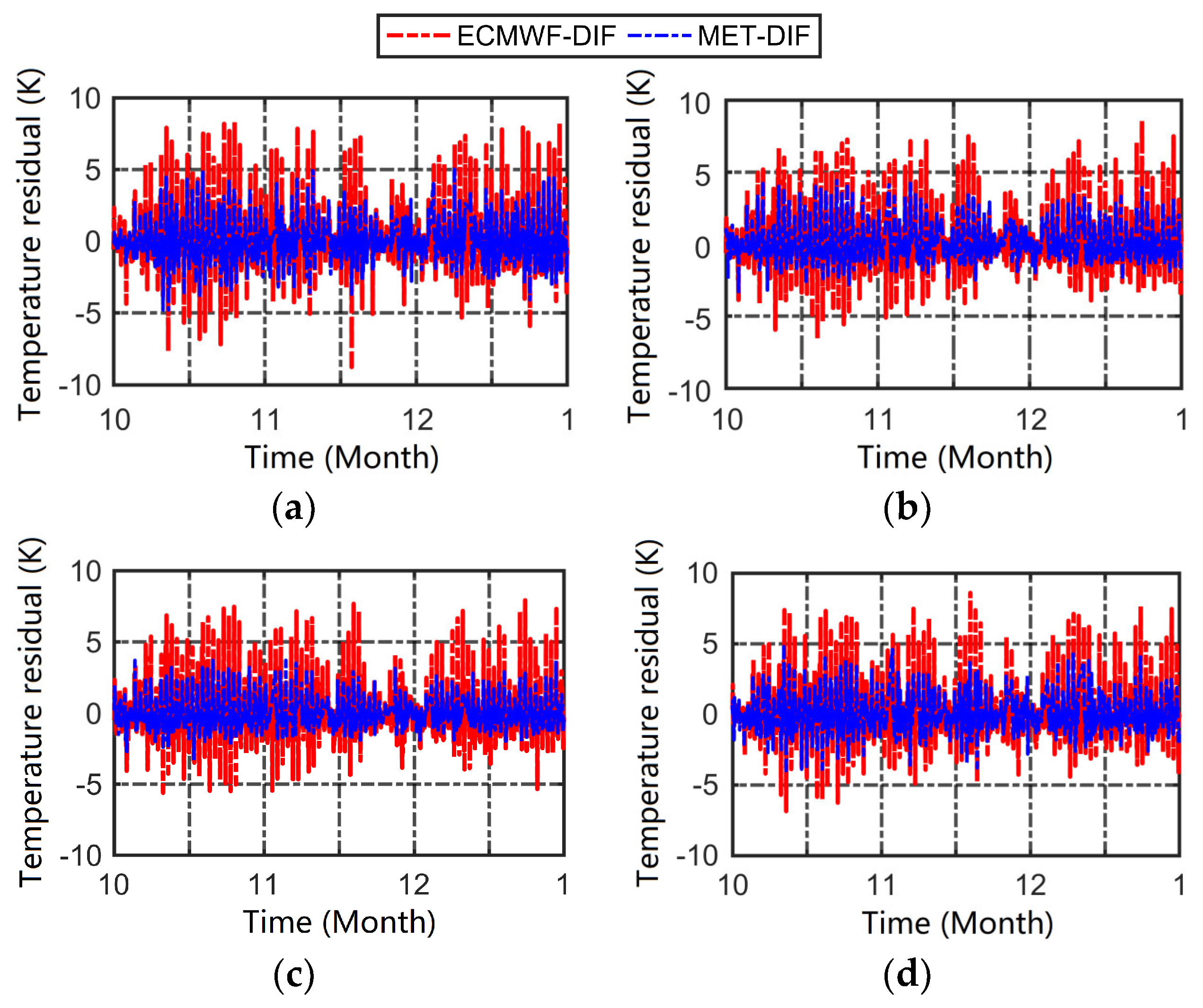
Figure 3 shows the temperature difference sequences (the red line) between the adjacent two hours before and after from 1 October to 31 December 2022 for four grid points with different elevations. The amplitude fluctuations were roughly distributed in the range of −9 to 9 K. Considering the TLR and the matching elevation bias of ASTER GDEM, the temperature differences of the neighboring epochs (the blue line in Figure 3) were calculated by interpolating the measured temperature values of the neighboring meteorological stations at the grid points using inverse distance-weighting. Figure 3 shows that both types of temperature difference time sequences had cusps. The measured temperature had significantly smaller cusps than the grid point, and the cusps occurred at the same time.
In order to quantitatively evaluate the differences in the FTC temperature in detail, the median values of the ERA5 and measured meteorological data at UTC 1–2 h, UTC 9–10 h and other epochs were collected: 5.47 K, 3.55 K and 0.99 K for the ERA5 data and 2.80 K, 2.33 K and 0.75 K for the meteorological observations, respectively. The differences in the median value of the two types of data in the three periods were 2.67 K, 1.21 K and 0.24 K, respectively. Therefore, in high-precision atmospheric temperature applications and modeling forecasts, the bias outliers of cusp data for the two periods need to be modeled and corrected. For the ERA5 2 m atmospheric temperature, the large cusp outliers were mainly related to the data assimilation model and forecasting algorithm used in the product generation [27]. The results show that the cusp outliers of the ERA5 2 m atmospheric temperature were due to the anomalously large raw data of the grid points at UTC 1 h and UTC 9 h. Therefore, a method based on partitioning polynomial fitting was proposed to correct the raw temperature data at UTC 1 h and UTC 9 h.
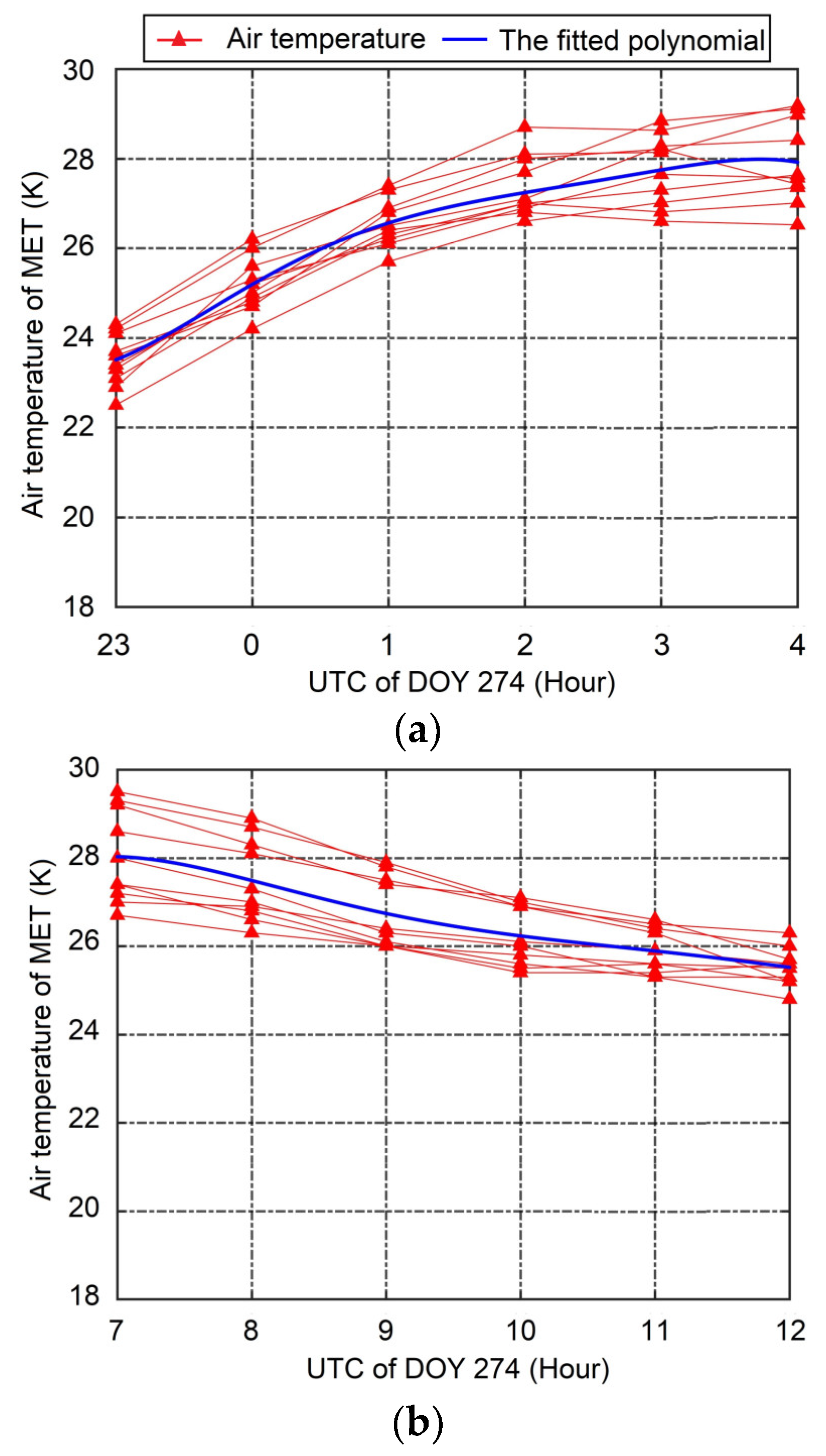
In a certain range, when the temperature values at different stations were corrected to the same elevation, the results tended to be very close. Thus, this study divided the study area at a resolution of 0.5° × 0.5°. There was an overlap of 0.25° between neighboring regions, and then a certain grid point was located in four regions at the same time. All the meteorological station data within the same area were converted to a specific elevation, which was calculated using the median elevation of all stations. Since the temperature changed smoothly in a certain period, without a sudden increase or decrease, this study took six hours as the polynomial fitting window to obtain the best-fit polynomials across the UTC 1 h and UTC 9 h cusp data, respectively. The principle of selecting the 6 h temperature data is to place the cusp epoch in the middle of the fitting period, and the order of the polynomial is determined by using the adaptive identification method. The polynomial fitting of the first partition is shown in Figure 4 as an example at the day of year (DOY) 274.
Based on the partitioning polynomial fitting correction method, we corrected the ERA5 2 m atmospheric grid temperature from 1 October to 31 December 2022 in Shandong Province. In order to evaluate the correction performance, the corrected grid data were interpolated to the meteorological stations using a bilinear interpolation method, considering the TLR and the EMB. Since only the temperature at the epochs of cusps were corrected during the model correction, the temperature data at UTC 1 h and UTC 9 h were counted in this analysis. The measured data at the meteorological stations were taken as the true values. The uncorrected and corrected temperature bias sequences at these two moments at four typical meteorological stations are shown in Figure 5 and Figure 6, respectively. The analysis shows that the ERA5 2 m atmospheric grid temperatures at UTC 1 h and UTC 9 h were significantly improved after correction using the partitioning polynomial fitting correction method. The temperature bias was relatively larger for the stations with relatively higher altitudes, with more significant improvement. The biases at UTC 1 h were larger than those at UTC 9 h, which were significantly reduced after model correction.
Table 2 summarizes the average RMS of temperature biases of all the meteorological stations at two epochs before and after the model correction at different elevations in order to analyze the improvement in UTC 1 h and UTC 9 h temperature values. The result shows that for the highest Taishan Mountain station, the average RMS at UTC 1 h and UTC 9 h decreased by 2.78 K and 2.11 K after model correction, with the accuracy improved by 61.0% and 47.3%, respectively. With the reduction in the elevation interval, the average RMS at UTC 1 h and UTC 9 h decreased by about 1.32 K and 1.19 K after model correction, respectively, with an accuracy improvement of about 48.4% and 50.6%, respectively. In addition, the analysis also shows that with the increase of elevation intervals, the temperature bias at these two moments before model correction gradually increased. When the model was corrected, the temperature biases at the two moments were basically at the same level in all the elevation intervals. Therefore, it is necessary to correct the UTC 1 h and UTC 9 h temperature values during the precise use of the ERA5 2 m atmospheric temperature. To ensure unbiased statistics, we used the three-sigma threshold for statistical RMS to remove the abnormal results.

4.3. Refinement of the ERA5 Gridded Temperature Model Based on the RRM

As shown in Table 1 and Table 2, although the TLR, MBS and FTC outliers were corrected, the ERA5 2 m temperature interpolated to the meteorological station still exhibited some biases from the actual measurement data, with an average of about 1.68 K and a maximum value of about 2.05 K. Therefore, we further proposed an atmospheric temperature correction model by using the RRM based on the above two methods.
The main modeling steps are as follows. (1) The remove step: the bilinear interpolation method was used to interpolate the ERA5 2 m atmospheric temperature to the meteorological stations and then the interpolated data and the situ measured data were used to calculate the corrected residuals at each meteorological station. (2) The restore step I: The spherical harmonic function model was used to expand the residuals calculated at each meteorological station and to calculate the spherical harmonic coefficient. Since the study area in this study is only included Shandong Province, the normalized spherical harmonic model was used (Equation (6)) [38,39]. (3) The restore step II: The spherical harmonic coefficient and the location information of the grid points were used to calculate the corrected temperature value. Then, the corrected temperature and the ERA5 2 m atmospheric temperature raw data were used to refine the temperature data at the grid points. It is worth noting that only 84 meteorological stations were used in the model. The highest point, Taishan Mountain and 24 stations in all elevation intervals below 350 m in Table 2 were excluded in the model correction, and were used to objectively assess the feasibility of the method. These 24 stations are evenly distributed across 4 elevation intervals.
The corrected 2 m gridded atmospheric temperature and 25 meteorological stations data excluded in the RRM were utilized to validate the method. Firstly, the temperature data of four grid points near the meteorological station were normalized to the elevation level of the meteorological station using the TLR and EMB correction method. The refined grid point temperature was interpolated to the meteorological station using the bilinear interpolation method and then compared with the measured data. Two schemes were used for the validation: with and without RRM correction.
Figure 7 shows the residual sequences under the two schemes at four typical meteorological stations at different elevations, with the measured data of the meteorological stations as the true values. The average STD of the temperature residuals before and after the model correction for the elevation intervals at the 25 meteorological stations are summarized in Table 3. The analysis shows that the availability of ERA5 2 m atmospheric temperature was significantly enhanced after the RRM-based model correction, and the enhancement of the grid temperature availability was more significant at higher elevations. Table 3 shows that, for the whole study area, the accuracy of the grid temperature was improved by about 18.4% on average after the refinement of the RRM. The highest meteorological station (The Taishan Mountain station) had the largest grid temperature improvement rate (about 35.3%). With the reduction of the elevation interval, the improvement in the availability of the grid temperature gradually decreased. For the elevation intervals between 0–50 m and 50–100 m, the temperature improvement rate still reached about 11.3%. Therefore, by constructing the RRM, the accuracy and availability of the ERA5 2 m atmospheric grid temperature data can be further improved.

5. Discussion

In order to verify the systematic and complete refinement method proposed by this study for the ERA5 2 m atmospheric grid temperature model, the usability and overall accuracy improvement performance were evaluated. Four solutions were set up to interpolate the atmospheric grid temperature to all the meteorological stations: (1) directly using the original ERA5 2 m atmospheric temperature (Solution A); (2) corrected by both the TLR and EMB (Solution B), corrected by the FTC method (Solution C) and corrected based on the RRM (Solution D). Solution D was implemented based on Solution C, and Solution C was based on Solution B.
Table 4 shows the average RMS of the temperature residual for the four schemes at different elevation intervals. In order to better demonstrate the reliability of the proposed method, the 2 m grid temperature above the surface of land from the National Centers for Environmental Prediction (NCEP)/National Center for Atmospheric Research (NCAR) reanalysis product was used for validation and comparison. Similar to solution A, the original grid temperature of the NCEP/NCAR was interpolated into the meteorological station, and the RMS calculated by comparing it with the true value was also included in Table 4 (Solution E). This type of assimilation data come from ground meteorological stations, radio sounding, sounding balloons, satellites, etc. Its atmospheric temperature at 2 m above the land surface also has a high accuracy. The spatial resolution and temporal resolution are 1.875° × 1.875° and 6 h, respectively. The analysis shows that the systematic grid temperature refinement method proposed in this study presented significant improvement in each step over the previous step. In particular, the complete 2 m atmospheric grid temperature refinement method showed the most significant improvement over the original ERA5 2 m atmospheric grid temperature data, and the average RMS of the temperature residual can be reduced to 0.57 K. For the highest point (the Taishan Mountain station), the RMS was reduced from 5.28 K to 0.76 K. In addition, by comparing Solution A and Solution E, it can be seen that the availability of temperature data for the ECMWF ERA5 in the current research area is slightly higher than those of the NCEP products. After the correction of the atmospheric grid temperature refinement method proposed in this study, the availability of ERA5 temperature data is significantly higher than that of the NCEP, and the improvement effect is more significant at higher altitudes. This result further proves the high reliability and availability of a systematic and complete refinement method for the ERA5 2 m atmospheric grid temperature model.
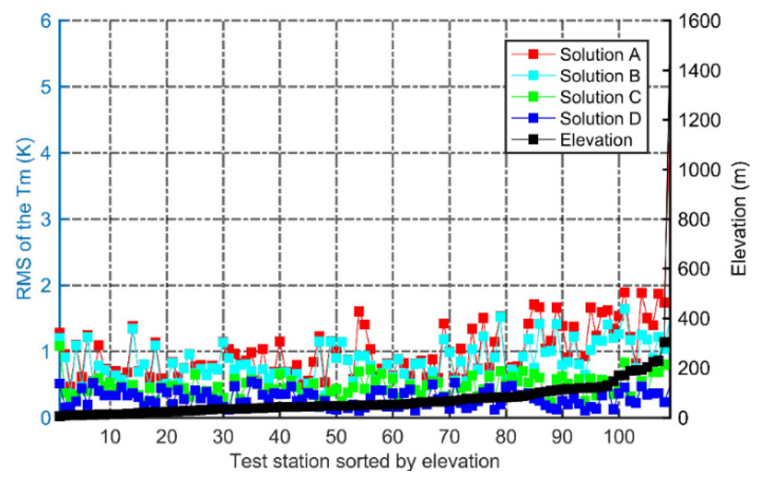
According to Yao et al., a linear transformation formula suitable for the eastern region of China was used to calculate the T m of interpolated temperature values for all meteorological stations in the region [37]. Taking the T m calculated from the measured temperature at the weather station as the reference value, the RMS values of the T m deviation for various schemes were calculated. The RMS statistics are presented in Figure 8 with Solution A, Solution B, Solution C and Solution D. The average RMS of the temperature values for the four schemes at different elevation intervals are given in Table 5. The analysis results indicate that for Solution A, the RMS of the T m gradually increases with the increase in altitude, and the applicability of ERA5 2 m grid temperature gradually decreases. When corrected using Solution B, Solution C and Solution D in sequence, the average RMS gradually decreases, and the availability of ERA5 2 m grid temperature increases sequentially. The complete refinement method (solution D) showed the most significant improvement, especially in high-altitude areas. The average RMS of the T m for all the stations could be reduced to 0.47 K. The RMS of the highest point (the Taishan Mountain station) could be reduced from 4.28 K to 0.62 K, and the RMS values of the meteorological stations at the remaining elevations were reduced to about 0.43 K. Therefore, the proposed overall refinement method that can be corrected by the EMB, FTC and RRM models in sequence can significantly improve the accuracy and usability of the ERA5 2 m atmospheric grid temperature in the T m inversion.
In order to further verify the usability of the overall refined ERA5 2 m atmospheric grid temperature in GNSS PWV calculation, three GNSS continuous tracking stations (SDGT, SD09 and SDZT) in the region were selected. Based on GAMIT/GLOBK software (http://geoweb.mit.edu/gg/, accessed on 14 September 2023), a 2 h resolution tropospheric wet delay in the zenith direction was calculated and obtained. In the processing process, the data of Global Positioning System and BeiDou Navigation Satellite System were used. The pressure at the GNSS stations was interpolated via nearby meteorological stations, and the modified Vienna mapping function (VMF3) and Saastamoinen were used [19].
SDGT, SD09 and SDZT are located 54.2 km, 48.6 km and 8.4 km away from the nearest meteorological stations 54826 (altitude 1533.7 m), 54836 (altitude 305.1 m) and 54945 (altitude 108.4 m), respectively, and the detailed spatial distribution is shown in Figure 1. Traditionally, there has been no significant change in the ZWD values within a distance of 50 km. Therefore, this study directly assumes that the ZWD in the zenith direction of the GNSS and meteorological stations is the same on the same elevation plane. The detailed calculation steps for the PWV at the meteorological station are as follows: (1) Convert and unify the ERA5 2 m atmospheric temperature, meteorological station and GNSS station elevation system; (2) According to Dousa and Elias [40] and Vaclavovic et al. [41], the ZWD at the GNSS station is converted to the elevation plane of the meteorological station, and the specific conversion is shown in Equation (7); (3) The Kriging interpolation method was used to interpolate the original and refined ERA5 2 m atmospheric temperature into the meteorological station, and the linear model recommended by Yao et al. was used to calculate the Tm [37]. The PWV in the zenith direction of the stations was then calculated, denoted as GNSS-PWV1 and GNSS-PWV2, respectively; (4) Calculate the GNSS PWV (GNSS-PWVr) using the same method based on the measured temperature at the meteorological station. Due to the lack of air sounding data in the study area, the PWV calculated based on actual temperature (GNSS-PWVr) was used as a reference value to evaluate and analyze the differences in and reliability of GNSS-PWV1 and GNSS-PWV2.
Z W D m = Z W D s · exp ( H m H s q z w d )
where Z W D s and Z W D m are the ZWD in the zenith direction of the GNSS and meteorological stations, respectively. H s and H m are the elevations of the GNSS stations and meteorological stations, respectively. q z w d is the height of the empirical scale, and the value was defined as 2 km.
Figure 9 shows the residual sequences of GNSS-PWVr minus GNSS-PWV1, as well as GNSS-PWVr minus GNSS-PWV2 for three stations, respectively. The RMS, mean absolute error (MAE) and maximum absolute error (MXAE) are summarized in Table 6. As shown in Figure 9 and Table 6, the accuracy of directly using the original ERA5 2 m atmospheric temperature to calculate the PWV is relatively poor, especially for meteorological station 54826 with a high altitude, where the RMS of the PWV residual is 0.662 mm and the maximum deviation is 3.947 mm, which has a significant impact on rainfall forecasting and GNSS meteorology research. However, after being corrected through the overall refinement method proposed in this study, the RMS and MXAE of PWV residuals were reduced to 0.203 mm and 1.390 mm, respectively, and the accuracy of PWV calculation was significantly improved. In addition, for the meteorological stations located at an altitude of 100–350 m, there is also a certain degree of improvement in accuracy when calculating the PWV using the ERA5 2 m atmospheric grid temperature model refined using the EMB, FTC and RRM methods. For meteorological stations 54836 and 54945, the RMS decreased by 0.124 mm and 0.097 mm, respectively, and the MXAE decreased by 1.178 mm and 1.031 mm, respectively. The results of this study are basically consistent with those of Huang et al. [18].

6. Conclusions

The ERA5 2 m surface atmospheric temperature reanalysis product has become an important data source in the fields of GNSS meteorology research, regional climate change simulation and validation and extreme weather forecasting due to its advantages of good release regularity, high spatiotemporal resolution and strong spatial topology. We evaluated the availability of the ERA5 2 m air temperature data in Shandong Province, China based on the regional measured data at meteorological stations and proposed a complete set of ERA5 2 m atmospheric temperature refinement methods. The proposed method included the EMB correction of temperature, correction of FTC temperature and overall refinement based on the RRM. This method can maintain the topology and high spatiotemporal resolution characteristics of the product while improving the regional applicability of ERA5. The main conclusions are as follows:
(1)
The applicability of the ERA5 2 m atmospheric temperature gradually decreased with the increase in the terrain altitude. Without any model correction, the comparison of the measured data from the meteorological stations at the altitudes of 1533 m (the highest) and 0–50 m (the lowest) revealed that the average RMS of temperature biases were 5.28 K and 1.09 K, respectively. After the correction of the TLR and EMB, the accuracy was improved by about 68.8% and 11.3% at the elevation of 1533 m and 0–50 m, respectively. Particularly, the accuracy improvement was more significant after the correction at higher elevations.
(2)
It was found that the grid temperature values at UTC 1 h and UTC 9 h had abnormally large biases from the measured values by deriving the differences between neighboring epochs. Thus, we proposed an adaptive partitioning polynomial fitting correction model based on the situ data to correct the grid temperature values at these two moments. The results show that the accuracy of the temperature values at UTC 1 h and UTC 9 h was improved by about 50.2% and 49.4% after the model correction, respectively.
(3)
The availability of ERA5 2 m atmospheric temperature data was significantly enhanced after the RRM-based model correction, and the enhancement of the grid temperature availability was more significant at higher elevations. For the whole study area, the accuracy of the grid temperature was improved by about 18.4% on average after the refinement of the RRM. The highest meteorological station (the Taishan Mountain station) had the largest grid temperature improvement rate of 35.3%.
(4)
When calculating the T m and PWV using the overall refinement ERA5 2 m atmospheric temperature, the average RMS of the T m could be reduced to 0.47 K in the whole region, and for the meteorological station 54826 with high altitude, the RMS was reduced from 4.28 K to 0.62 K. For the PWV at meteorological station 54826 with a high altitude, the RMS is decreased by 69.3% from 0.662 mm to 0.203 mm, and the MXAE reduced by 2.563 mm. For the meteorological stations located at an altitude of 100–350 m, the RMS of the PWV residual decreased by 52.2% from 0.211 mm to 0.101 mm, and the MXAE reduced by 1.264 mm.

Author Contributions

Conceptualization, C.Y. and H.W.; methodology, C.Y.; software, C.Y.; validation, C.X.; formal analysis, C.Y.; investigation, H.W.; resources, C.Y.; data curation, C.Y.; writing—original draft preparation, C.Y.; writing—review and editing, C.X.; visualization, C.Y.; supervision, H.W.; project administration, C.X.; funding acquisition, C.Y. All authors have read and agreed to the published version of the manuscript.

Funding

This research was funded by the National Natural Science Foundation of China, grant number 42274044, 41874042,41974010 and the State Key Laboratory of Geo-Information Engineering and Key Laboratory of Surveying and Mapping Science and Geospatial Information Technology of MNR, the Chinese Academy of Surveying and Mapping, grant number 2023-01-06.

Data Availability Statement

The ERA5 and NCEP/NCAR 2 m atmospheric temperature reanalysis data are available at https://cds.climate.copernicus.eu/ (accessed on 12 May 2023) and https://rda.ucar.edu/ (accessed on 14 May 2023). The in situ meteorological data for evaluating the 2 m atmospheric temperature and establishing a refinement model are available at https://cds.climate.copernicus.eu/ (accessed on 8 May 2023). The ASTER GDEM is available at https://gdemdl.aster.jspacesystems.or.jp/index_en.html (accessed on 1 June 2023). All the data and products are publicly available through the websites of the respective organizations except for in situ meteorological data.

Acknowledgments

The contribution of data from the ECMWF, NCEP/NCAR, China Meteorological Data Center, Crustal Movement Observation Network of China and NASA are appreciated.

Conflicts of Interest

The authors declare no conflicts of interest.

References

  1. Kiehl, J.; Trenberth, K. Earth’s annual global mean energy budget. Bull. Am. Meteorol. Soc. 1997, 78, 197–208. [Google Scholar] [CrossRef]
  2. Wang, J.; Zhang, L. Climate applications of a global, 2-hourly atmospheric precipitable water dataset derived from IGS tropospheric products. J. Geod. 2009, 83, 209–217. [Google Scholar] [CrossRef]
  3. Franco, L.; Almeida, C.; Freire, M.; Franco, G.; Silva, S. Rainfall zoning for cocoa growing in Bahia State (Brazil) using fuzzy logic. Eng. Agrícola 2019, 39, 48–55. [Google Scholar] [CrossRef]
  4. Jin, S.; Luo, O. Variability and climatology of PWV from global 13-year GPS observations. IEEE T Geosci. Remote Sens. 2009, 47, 1918–1924. [Google Scholar] [CrossRef]
  5. Wu, J.; Su, M.; Shen, X.; Qiao, L.; Zheng, J. Assessment of the performance of GPS-PWV and rainfall event prediction by using precise products from different analysis centers. Earth Sci. Inform. 2023, 16, 2199–2210. [Google Scholar] [CrossRef]
  6. Zhang, W.; Zhang, H.; Liang, H.; Lou, Y.; Cai, Y.; Cao, Y.; Zhou, Y.; Liu, W. On the suitability of ERA5 in hourly GPS precipitable water vapor retrieval over China. J. Geod. 2019, 93, 1897–1909. [Google Scholar] [CrossRef]
  7. Yao, Y.; Liu, C.; Xu, C.; Tan, Y.; Khan, S. A refined tomographic window for GNSS-derived water vapor tomography. Remote Sens. 2020, 12, 2999. [Google Scholar] [CrossRef]
  8. Zhao, Q.; Yao, Y.; Yao, W.; Li, Z. Near-global GPS-derived PWV and its analysis in the El Niño event of 2014–2016. J. Atmos. Sol. Terr. Phys. 2018, 179, 69–80. [Google Scholar] [CrossRef]
  9. Bevis, M.; Businger, S.; Chiswell, S.; Herring, T.; Anthes, R.; Rocken, C.; Ware, R. GPS Meteorology: Mapping Zenith Wet Delays onto Precipitable Water. J. Appl. Meteorol. 1994, 33, 379–386. [Google Scholar] [CrossRef]
  10. Huang, L.; Mo, Z.; Xie, S.; Liu, L.; Chen, J.; Kang, C.; Wang, S. Spatiotemporal characteristics of GNSS-derived precipitable water vapor during heavy rainfall events in Guilin, China. Satell. Navig. 2021, 2, 13. [Google Scholar] [CrossRef]
  11. Zhu, H.; Chen, K.; Chai, H.; Ye, Y.; Liu, W. Characterizing extreme drought and wetness in Guangdong, China using global navigation satellite system and precipitation data. Satell. Navig. 2024, 5, 1. [Google Scholar] [CrossRef]
  12. Zhang, B.; Yao, Y.; Xu, C. Global empirical model for estimating water vapor scale height. Acta Geod. Cartogr. 2015, 44, 1085–1091. (In Chinese) [Google Scholar]
  13. Bevis, M.; Businger, S.; Herring, T.; Rocken, C.; Anthes, R.; Ware, R. GPS meteorology: Remote sensing of the atmospheric water vapor using the global positioning system. J. Geophys. Res. 1992, 97, 15787–15801. [Google Scholar] [CrossRef]
  14. Niell, A.; Coster, A.; Solheim, F.; Mendes, V.; Toor, P.; Langley, R.; Upham, C. Comparison of measurements of atmospheric wet delay by radiosonde, water vapor radiometer, GPS, and VLBI. J. Atmos. Ocean. Technol. 2001, 18, 830–850. [Google Scholar] [CrossRef]
  15. Wang, J.; Zhang, L.; Dai, A.; Van, H.; Van, B. A near-global, 2-hourly data set of atmospheric precipitable water from ground-based GPS measurements. J. Geophys. Res. Atmos. 2007, 112, 7529. [Google Scholar] [CrossRef]
  16. Vázquez, B.; Grejner-Brzezinska, D. GPS-PWV estimation and validation with radiosonde data and numerical weather prediction model in Antarctica. GPS Solut. 2013, 17, 29–39. [Google Scholar] [CrossRef]
  17. Huang, L.; Liu, Z.; Peng, H.; Xiong, S.; Zhu, G.; Chen, F.; Liu, L.; He, H. A Novel Global Grid Model for Atmospheric Weighted Mean Temperature in Real-Time GNSS Precipitable Water Vapor Sounding. IEEE J. Sel. Top. Appl. Earth Obs. Remote Sens. 2023, 16, 3322–3335. [Google Scholar] [CrossRef]
  18. Huang, L.; Liu, W.; Mo, Z.; Zhang, H.; Li, J.; Chen, F.; Liu, L.; Jiang, W. A new model for vertical adjustment of precipitable water vapor with consideration of the time-varying lapse rate. GPS Solut. 2023, 27, 170. [Google Scholar] [CrossRef]
  19. Saastamoinen, J. Atmospheric correction for the troposphere and stratosphere in radio ranging satellites. Use Artif. Satell. Geod. 1972, 15, 247–251. [Google Scholar]
  20. Boehm, J.; Werl, B.; Schuh, H. Troposphere mapping functions for GPS and very long baseline interferometry from European Centre for Medium-Range Weather Forecasts operational analysis data. J. Geophys. Res. Solid. Earth 2006, 111, 3629. [Google Scholar] [CrossRef]
  21. Hagemann, S.; Bengtsson, L.; Gendt, G. On the determination of atmospheric water vapor from GPS measurements. J. Geophys. Res. 2003, 108, 3235. [Google Scholar] [CrossRef]
  22. Ning, T.; Wang, J.; Elgered, G.; Dick, G.; Wickert, J.; Bradke, M.; Sommer, M.; Querel, R.; Smale, D. The uncertainty of the atmospheric integrated water vapour estimated from GNSS observations. Atmos. Meas. Tech. 2016, 9, 79–92. [Google Scholar] [CrossRef]
  23. Epeloa, J.; Meza, A. Total column water vapor estimation over land using radiometer data from SAC-D/Aquarius. Adv. Space Res. 2017, 61, 1025–1034. [Google Scholar] [CrossRef]
  24. Kanamitsu, M.; Ebisuzaki, W.; Woollen, J.; Yang, S.; Hnilo, J.; Fiorino, M.; Potter, G. NCEP-DOE AMIP-II Reanalysis (R-2). Bull. Amer. Meteor. Soc. 2002, 83, 1631–1643. [Google Scholar] [CrossRef]
  25. Molod, A.; Takacs, L.; Suarez, M.; Bacmeister, J. Development of the GEOS-5 atmospheric general circulation model: Evolution from MERRA to MERRA2. Geosci. Model. Dev. 2015, 8, 1339–1356. [Google Scholar] [CrossRef]
  26. Hiroyuki, T.; Shogo, U.; Hideyuki, N.; Justin, S.; Kim, W.; Yeager, S.; Danabasoglu, G.; Suzuki, T.; Bamber, J.; Bentsen, M.; et al. JRA-55 based surface dataset for driving ocean–sea-ice models (JRA55-do). Ocean Model. 2018, 130, 79–139. [Google Scholar]
  27. Hersbach, H.; Bell, B.; Berrisford, P.; Hirahara, S.; Horányi, A.; Muñoz-Sabater, J.; Nicolas, J.; Peubey, C.; Radu, R.; Schepers, D.; et al. The ERA5 global reanalysis. Q. J. R. Meteorol. Soc. 2020, 146, 1999–2049. [Google Scholar] [CrossRef]
  28. Samuel, J.; Claudia, V.; Claudia, D.; Mirko, D.; Henny, A. Heatwaves, droughts, and fires: Exploring compound and cascading dry hazards at the pan-European scale. Environ. Int. 2020, 134, 105276. [Google Scholar] [CrossRef]
  29. Chen, Y.; Sharma, S.; Zhou, X.; Yang, K.; Li, X.; Niu, X.; Hu, X.; Khadka, N. Spatial performance of multiple reanalysis precipitation datasets on the southern slope of central Himalaya. Atmos. Res. 2021, 250, 105365. [Google Scholar] [CrossRef]
  30. Dee, D.P.; Uppala, S.; Simmons, A.; Vitart, F. The ERA-Interim reanalysis: Configuration and performance of the data assimilation system. Q. J. R. Meteorol. Soc. 2011, 137, 553–597. [Google Scholar] [CrossRef]
  31. Zhang, W.; Lou, Y.; Haase, J.; Zhang, R.; Zheng, G.; Huang, J.; Shi, C.; Liu, J. The use of ground-based GPS precipitable water measurements over China to assess radiosonde and ERA-Interim moisture trends and errors from 1999 to 2015. J. Clim. 2017, 30, 7643–7667. [Google Scholar] [CrossRef]
  32. Reuten, C.; Moore, R.; Clarke, G. Quantifying differences between 2 m temperature observations and reanalysis pressure level temperatures in northwestern North America. J. Appl. Meteorol. Climatol. 2011, 50, 916–929. [Google Scholar] [CrossRef]
  33. Zhou, C.; He, Y.; Wang, K. On the suitability of current atmospheric reanalyses for regional warming studies over China. Atmos. Chem. Phys. 2018, 18, 8113–8136. [Google Scholar] [CrossRef]
  34. Zhao, T.; Guo, W.; Fu, C. Calibrating and evaluating reanalysis surface temperature error by topographic correction. J. Clim. 2008, 21, 1440–1446. [Google Scholar] [CrossRef]
  35. Ferreira, V.; Freitas, S. Geopotential numbers from GPS satellite surveying and disturbing potential model: A case study of parana, brazil. J. Appl. Geod. 2011, 5, 155–162. [Google Scholar] [CrossRef]
  36. Wang, W.; Zhang, C.; Liang, S.; Yang, Q.; Hu, M.; Feng, W. Monitoring of the temporal and spatial variation of groundwater storage in the three gorges area based on the CORS network. J. Appl. Geophys. 2017, 146, 160–166. [Google Scholar] [CrossRef]
  37. Yao, Y.; Zhang, B.; Xu, C.; Chen, J. Analysis of the global Tm−Ts correlation and establishment of the latitude-related linear model. Chin. Sci. Bull. 2014, 59, 2340–2347. [Google Scholar] [CrossRef]
  38. Jin, R.; Jin, S.; Feng, G. M_DCB: Matlab code for estimating GNSS satellite and receiver differential code biases. GPS Solut. 2012, 16, 541–548. [Google Scholar] [CrossRef]
  39. Zhou, C.; Yang, L.; Li, B.; Balz, T. M_GIM: A MATLAB-based software for multi-system global and regional ionospheric modeling. GPS Solut. 2023, 27, 3709. [Google Scholar] [CrossRef]
  40. Dousa, J.; Elias, M. An improved model for calculating tropospheric wet delay. Geophys. Res. Lett. 2014, 41, 4389–4397. [Google Scholar] [CrossRef]
  41. Vaclavovic, P.; Dousa, J.; Elias, M.; Kostelecky, J. Using external tropospheric corrections to improve gnss positioning of hot-air balloon. GPS Solut. 2017, 21, 1479–1489. [Google Scholar] [CrossRef]
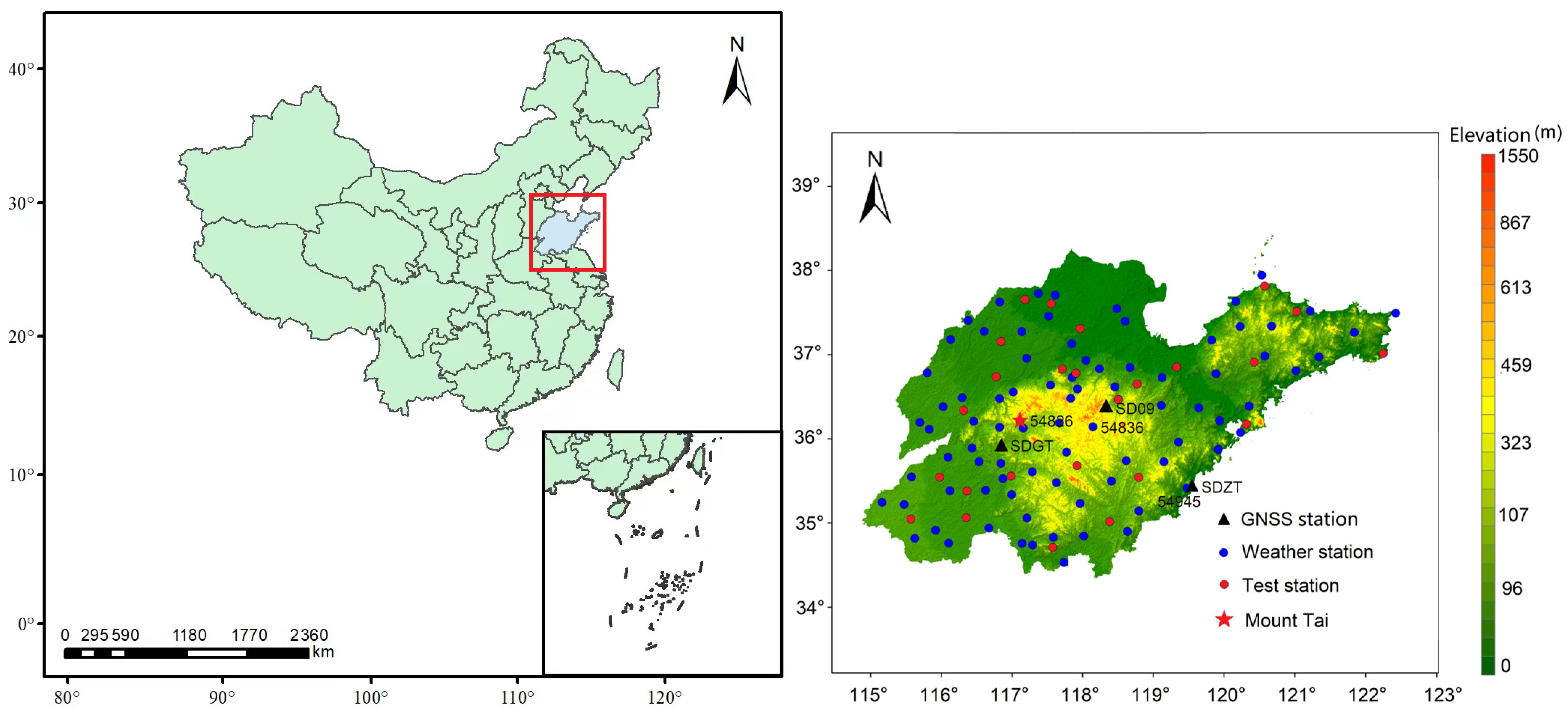
Figure 1. Topography and distribution of meteorological stations in Shandong Province, China. A total of 109 meteorological stations in the region from the China Meteorological Data Center were collected with a temporal resolution of 1 h. The hourly ERA5 atmospheric temperature data at 2 m above the land surface in Shandong Province were downloaded and cropped, with a total of 328 grid points. The Advanced Spaceborne Thermal Emission and Reflection Radiometer Global Digital Elevation Model (ASTER GDEM) was used to minimize the height difference between the reanalysis data and the actual meteorological observations.
Remotesensing 16 02055 g001
Figure 2. Temperature residual sequences for the four different meteorological stations under the three schemes. The latitude (°), longitude (°) and elevation (m) of (a) (36.25, 117.10, 1533.70), (b) (37.32, 120.85, 205.50), (c) (35.43, 119.53, 37.10) and (d) (36.42, 115.97, 34.30).
Remotesensing 16 02055 g002
Figure 3. Difference sequences of adjacent epochs for the atmospheric temperature between ERA5 and meteorological stations from 1 October 1 to 31 December 2022. The latitude (°), longitude (°) and elevation (m) of (a) (36.25, 117.10, 1533.70), (b) (37.32, 120.85, 205.50), (c) (35.43, 119.53, 37.10) and (d) (36.42, 115.97, 34.30).
Remotesensing 16 02055 g003
Figure 4. Best-fit polynomials. (a) UTC 1 h (top); (b) UTC 9 h.
Remotesensing 16 02055 g004
Figure 5. Bias sequences of temperature at UTC 1 h before and after model correction at four different elevation meteorological stations. The latitude (°), longitude (°) and elevation (m) of (a) (36.25, 117.10, 1533.70), (b) (37.32, 120.85, 205.50), (c) (35.43, 119.53, 37.10) and (d) (36.42, 115.97, 34.30).
Remotesensing 16 02055 g005
Figure 6. Bias sequences of temperature at UTC 9 h before and after model correction at four different elevation meteorological stations. The latitude (°), longitude (°) and elevation (m) of (a) (36.25, 117.10, 1533.70), (b) (37.32, 120.85, 205.50), (c) (35.43, 119.53, 37.10) and (d) (36.42, 115.97, 34.30).
Remotesensing 16 02055 g006
Figure 7. Residual sequence of the meteorological stations at different elevations before and after the RRM refinement. The latitude (°), longitude (°) and elevation (m) of (a) (36.25, 117.10, 1533.70), (b) (37.32, 120.85, 205.50), (c) (35.43, 119.53, 37.10) and (d) (36.42, 115.97, 34.30).
Remotesensing 16 02055 g007
Figure 8. Bias sequences at the interpolated meteorological stations for ERA5 2 m atmospheric temperature under the four schemes with increasing meteorological station elevations.
Remotesensing 16 02055 g008
Figure 9. Residual sequence of the PWV at the meteorological stations. (a) 54826; (b) 54836; (c) 54945.
Remotesensing 16 02055 g009
Table 1. The average RMS of the temperature residual for all meteorological stations with different elevations under the three schemes.
Elevation Interval (m)Refinement Strategy
Solution A (K)Solution B (K)Solution C (K)
15335.283.561.98
150~3102.071.661.57
100~1501.721.451.43
50~1001.331.211.18
0~501.091.011.01
Table 2. Average RMS of temperature bias at UTC 1 h and UTC 9 h before (Uncorr.) and after (Corr.) model correction for different elevation intervals (K).
Elevation Interval (m)UTC 1 hUTC 9 h
Uncorr.Corr.Uncorr.Corr.
15335.402.353.682.06
150~3104.072.183.371.87
100~1503.321.993.101.65
50~1002.881.662.661.53
0~502.811.592.451.36
Table 3. Average STD of the residual series of grid temperature at different elevation intervals before and after the RRM refinement.
Elevation Interval (m)Corrections without Using the RRM (K)Corrections Using the RRM (K)Enhancement Rate (%)
15331.060.7628.3
150~3100.840.6917.9
100~1500.760.6514.5
50~1000.680.5913.2
0~500.650.5810.8
Table 4. Average RMS at the interpolated meteorological stations for atmospheric temperature under different elevation intervals.
Elevation (m)Solution A (K)Solution B (K)Solution C (K)Solution D (K)Solution E (K)
15335.281.981.060.765.79
150~3102.041.550.830.582.37
100~1501.691.440.760.541.87
50~1001.311.160.730.531.39
0~501.081.020.690.481.16
Table 5. Average RMS at interpolated meteorological stations for the T m under the four schemes for different elevation intervals.
Elevation Interval (m)Solution A (K)Solution B (K)Solution C (K)Solution D (K)
15334.281.600.820.62
150~3101.681.270.680.48
100~1501.391.160.630.45
50~1001.080.960.600.42
0~500.880.820.580.41
Table 6. Accuracy of the PWV at the three meteorological stations.
Meteorological StationsWithout Correction (mm)With EMB, FTC and RRM Correction (mm)
RMSMAEMXAERMSMAEMXAE
548260.6620.4313.9470.2030.1281.390
548360.2210.0942.5320.0970.0481.153
549450.2020.1001.7900.1050.0510.758
Disclaimer/Publisher’s Note: The statements, opinions and data contained in all publications are solely those of the individual author(s) and contributor(s) and not of MDPI and/or the editor(s). MDPI and/or the editor(s) disclaim responsibility for any injury to people or property resulting from any ideas, methods, instructions or products referred to in the content.