Abstract
Small object detection poses significant challenges in the realm of general object detection, primarily due to complex backgrounds and other instances interfering with the expression of features. This research introduces an uncomplicated and efficient algorithm that addresses the limitations of small object detection. Firstly, we propose an efficient cross-scale feature fusion attention module called ECFA, which effectively utilizes attention mechanisms to emphasize relevant features across adjacent scales and suppress irrelevant noise, tackling issues of feature redundancy and insufficient representation of small objects. Secondly, we design a highly efficient convolutional module named SEConv, which reduces computational redundancy while providing a multi-scale receptive field to improve feature learning. Additionally, we develop a novel dynamic focus sample weighting function called DFSLoss, which allows the model to focus on learning from both normal and challenging samples, effectively addressing the problem of imbalanced difficulty levels among samples. Moreover, we introduce Wise-IoU to address the impact of poor-quality examples on model convergence. We extensively conduct experiments on four publicly available datasets to showcase the exceptional performance of our method in comparison to state-of-the-art object detectors.
1. Introduction
The objective of object detection is to classify and precisely locate objects, with small object detection (SOD) representing a distinct subdomain that emphasizes the identification of small-sized objects [1]. SOD finds extensive applications in various domains, including natural resource surveys, environmental monitoring, disaster management, agriculture, autonomous driving, and military applications. In recent years, there has been significant advancement in the domain of small object detection, thanks to the utilization of convolutional neural networks (CNN) in deep learning approaches. However, despite these exciting advancements, SOD continues to present challenges in object detection research. For example, the state-of-the-art detector YOLOv7 [2] achieved an average precision (mAP) of 56.0 and 66.7 on medium and large instances in the COCO test set. Still, its performance dropped significantly to 35.2 when dealing with small objects. This performance gap can be attributed not only to the typical obstacles encountered in general object detection, including occlusions and lighting variations, but also to specific issues inherent to SOD. Specifically, existing feature extractors [3,4,5,6,7,8] have limitations in representing features for small objects, as conventional downsampling operations result in the deprivation of details associated with small objects, and small object features are susceptible to contamination from backgrounds and other instances, making it challenging for networks to capture the discriminative information required for subsequent tasks. Furthermore, the problem of sample imbalance between easy and difficult examples causes models to overlook the learning of regular samples and challenging ones during the optimization process, further affecting SOD performance. Small objects also exhibit lower tolerance to bounding box perturbations compared to larger objects, which can impact the model’s convergence. Overcoming the challenges of small object detection requires overcoming these limitations, enhancing feature representation quality, and reducing interference from other factors.
Currently, in two-stage detection algorithms (e.g., ref. [9,10,11]), the process of object detection is executed through iterative refinement steps. Initially, these algorithms utilize a specially designed region proposals network (RPN) to generate high-quality candidate boxes. Subsequently, these candidate regions undergo classification and position regression. In contrast, one-stage detection algorithms conduct detection in a solitary step, showcasing enhanced computational efficiency by eliminating the requirement for an RPN. One-stage object detection algorithms are mainly divided into SSD ([12,13]) and YOLO ([5,14,15,16,17,18]) as the mainstream. The YOLO series is widely recognized in industrial applications for its impressive balance of detection accuracy and speed. For instance, ref. [14] introduced DarkNet-19 as a backbone network and integrated batch normalization preprocessing, higher-resolution classifiers, multi-scale training mechanisms, and binary cross-entropy loss functions, resulting in significant improvements in recall and accuracy. Nonetheless, there are still possibilities for further improving the detection capability of small objects. The deeper DarkNet-53 residual network was adopted in their work [5], along with an FPN (feature pyramid network), more scales of feature maps, and additional anchor points to enhance small object detection performance. Nevertheless, this led to an increase in model complexity. Ref. [19] introduced a cascade query strategy aimed at eliminating redundant computations on low-level features. Ref. [16] incorporated CSPDarkNet53, SPP+PAN fused features, data augmentation, and DropBlock regularization, resulting in significantly improved detection accuracy while maintaining speed. Ref. [20] proposed an efficient rep-style Gaussian–Wasserstein network (ERGW-net), which effectively addressed the challenges of small object sizes and low contrast in infrared aerial imagery. Ref. [17] introduced mosaic data augmentation, focus, CSP structure, and GIoU loss functions, offering fast inference speed and powerful detection performance. Incorporating attention mechanisms at the pixel and channel levels [21], this design aimed to enhance the feature information of small objects, simultaneously suppressing background noise. Furthermore, ref. [22] proposed a novel metric, dot distance, to mitigate the sensitivity of IoU (intersection over union) boundary box losses. Additionally, ref. [23] proposed NWD (normalized Wasserstein distance) and ref. [24] proposed a novel loss function that does not require additional computation or time cost during inference, thereby enhancing the localization accuracy of small objects, which improves the detection capability for small objects.
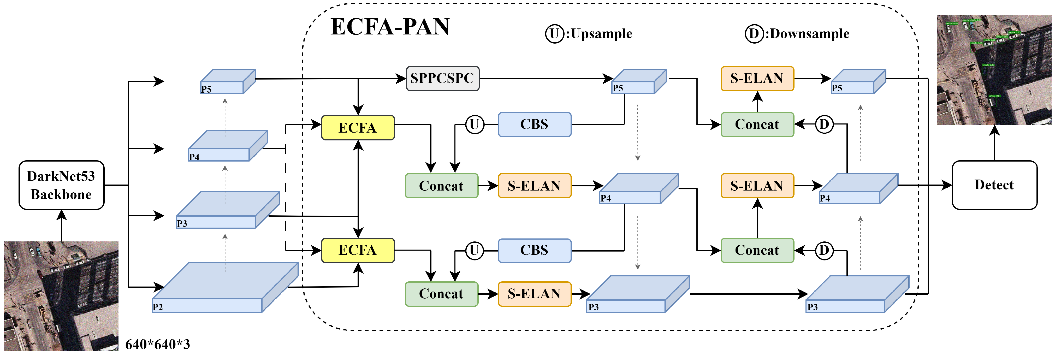
To tackle the challenges posed by complex background interference, diverse object scales, and performance bottlenecks of existing detectors in handling small objects, we introduce fine-grained feature enhancement for small object detection (FFEDet) within a comprehensive architectural framework depicted in Figure 1. Small objects often become obscured within intricate backgrounds, making it challenging for single-scale feature extraction to fully capture these targets. To efficiently fuse features across different scales, we propose the effective cross-scale feature fusion attention (ECFA) module. Leveraging attention mechanisms, this module adeptly integrates features from various scales, better capturing the details and contextual information of small objects while emphasizing relevant features and suppressing irrelevant noise. This cross-scale fusion enriches feature representation and enhances the model’s robustness to complex backgrounds. Another critical challenge in small object detection is maintaining efficient computation while boosting feature extraction capability. Thus, we introduce the simple yet efficient convolution (SEConv) module, which reduces computational redundancy and provides multiscale receptive fields, thereby enhancing feature learning capacity. During training, due to uneven sample distribution, the contributions of different samples to the model should dynamically vary. To address this, we propose the dynamic focal sample weighting function (DFSLoss), which dynamically adjusts the focus on optimizing normal and challenging samples during model training. By reducing the impact of simple samples on loss, this function enhances algorithm effectiveness. Furthermore, in the detection process, low-quality samples can adversely affect model performance. Hence, we incorporate Wise-IoU as the localization loss function to alleviate the sensitivity of detection boxes to IoU. Implementing this strategy helps mitigate the negative impact of low-quality samples, facilitating better model convergence.
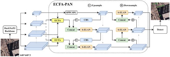
Figure 1.
The whole pipeline of the proposed FFEDet. Utilization of DarkNet53 as the primary network architecture for feature extraction at four distinct levels. The extracted features are further enhanced using ECFA-PAN to improve their quality. Finally, we conduct object detection on three feature maps that contain rich semantic information at varying levels.
This paper offers the following key contributions:
- We present the efficient cross-scale information fusion attention (ECFA) module, which efficiently fuses information across different scales through attention mechanisms. This module effectively reduces feature redundancy while improving the representation of small objects;
- We develop SEConv, a simple and highly efficient convolutional module that effectively reduces computational redundancy and provides multi-scale receptive fields, resulting in enhanced feature learning capabilities;
- We design DFSLoss, a dynamic focal sample weighting function, to overcome the issue of imbalanced hard and easy samples and improve network model optimization. Moreover, we introduce Wise-IoU to alleviate the negative effects of poor-quality examples on model convergence.
2. Related Work
2.1. Scale-Aware Methods
In image processing applications, objects typically exist at various scales, especially in fields such as traffic monitoring and remote sensing, posing significant challenges for single detectors. Traditional handcrafted feature-based methods often perform poorly in detecting small objects due to their limited feature representation capability. Early deep learning detection methods, primarily relying on high-level features, similarly struggle to effectively capture the details of small objects. To address this issue, multiscale detection strategies have been developed to enhance the recognition of small objects. For example, ref. [25] assumed that information within regions of interest (RoI) can be distributed across different layers of the backbone network, necessitating an effective organization strategy. By combining and integrating features from larger to smaller scales, this method obtains hyper-features that retain the capability to identify small objects. However, this approach may perform poorly in complex backgrounds, as the fusion of features from different layers can introduce extraneous background information. Ref. [26] employed scale-dependent pooling (SDP) to determine the optimal feature layers for aggregation. Although this method can adaptively select the feature layers best suited for small objects, it may lead to information loss during the multiscale feature aggregation process. This issue is particularly pronounced in scenes with objects of varying scales, potentially resulting in reduced detection performance. Ref. [27] generates detection proposals at various intermediate layers, with each layer specializing in objects within a specific scale range. While this method optimizes sensitivity to small objects, the primary issue is the lack of feature sharing between layers, resulting in insufficient overall feature representation. When objects in a scene exhibit significant scale variation, insufficient coordination between layers may affect detection performance. Ref. [12] proposed identifying small targets on high-resolution feature maps, leveraging the rich detail contained within these maps. The main problem with this approach is that high-resolution feature maps are susceptible to noise and background information during processing, leading to increased false detection rates. Additionally, the generation and processing of high-resolution feature maps demand high data quality, and low-quality images can severely impact detection performance. Ref. [15] adopted parallel branches for multiscale prediction, utilizing high-resolution feature maps to handle small objects. The main issue with this method is inadequate feature fusion and information sharing between branches, potentially resulting in poor coordination of the overall detection system. Moreover, the design of parallel branches requires careful consideration of each branch’s feature extraction capability and detection accuracy to avoid performance imbalances between branches. Inspired by [28,29], a connection was established between RoIs and a fusion of pooled features at various scales along with global features. This approach effectively combines local and global information, enhancing the robustness of small object detection. However, the fusion of features at different scales requires highly precise design and tuning, with extensive experimentation needed to determine appropriate weight distribution and fusion strategies. Additionally, the selection of RoIs and the precise matching of pooled features are critical issues; any misalignment may lead to suboptimal detection performance. In summary, although various multiscale detection strategies have significantly improved small object detection performance, challenges remain in feature fusion, information sharing, noise filtering, and scene adaptability.
2.2. Feature Fusion Methods
Deep convolutional neural networks (deep CNNs) generate hierarchical feature maps with varying spatial resolutions. These networks leverage low-level features to capture fine details, thereby providing accurate localization cues, while high-level features extract semantic information, enhancing representation. However, downsampling layers in deep feature maps can diminish their responsiveness to small objects. To address this issue, recent research has adopted feature fusion strategies that integrate multi-level features to obtain higher-quality representations for small objects. For instance, ref. [30] employed a hierarchical approach with lateral connections to combine features at different scales, capturing fine-grained details and semantic information to enhance small object detection. While this method effectively integrates features from different levels, it may struggle in complex scenes where lateral connections fail to adequately fuse low and high-level features, resulting in decreased detection accuracy. Additionally, this approach requires the precise alignment of feature maps, and misalignment can lead to significant performance issues. Building on FPN, ref. [28] introduced a bottom-up pathway to address gradient inconsistency issues found in FPN-based methods, thereby enhancing the representational capacity of lower-level features. Although this improvement enhances gradient propagation and strengthens low-level feature representation, it may introduce noise and irrelevant information in highly dense scenes, negatively impacting overall detection performance. Moreover, ref. [9] aggregated features at multiple spatial scales to accommodate objects of different sizes. While this method improves detection performance across various scales, it can encounter feature confusion when dealing with objects that have significant scale variation, especially when objects fall near the boundary of the fused features’ scales. In summary, feature fusion methods have made significant strides in mitigating the spatial and semantic discrepancies between low and high-level pyramid layers. However, challenges remain in capturing the fine-grained details crucial for the accurate localization and classification of small objects. Issues such as background noise, feature misalignment, and feature confusion in complex scenes continue to pose problems. Future research needs to optimize feature fusion strategies further to ensure stable and efficient small object detection across diverse and complex scenarios.
2.3. Context Modeling Methods
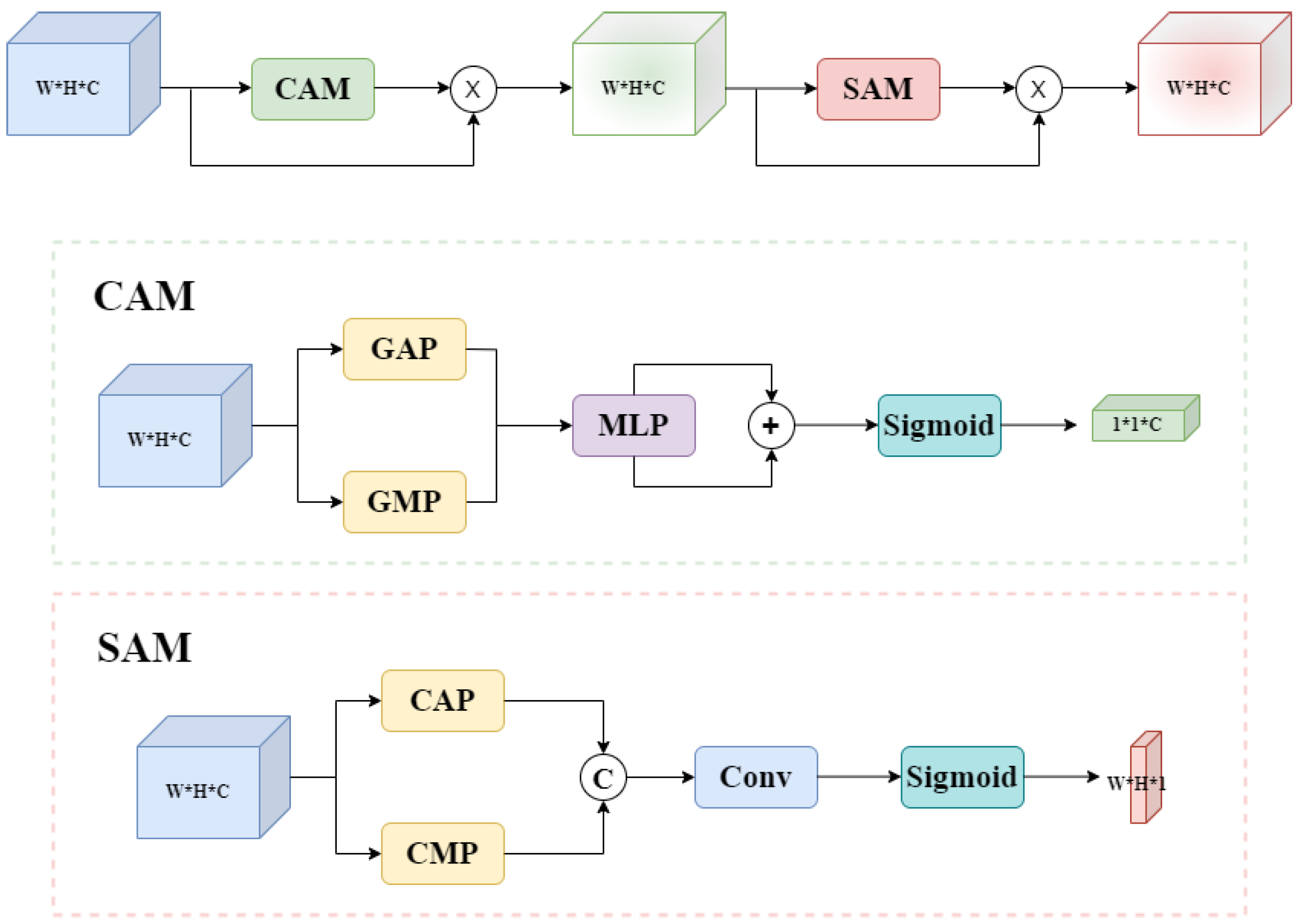
Context modeling methods aim to enhance the performance of salient object detection (SOD) by integrating contextual information and leveraging the correlation between objects and their surrounding environment to boost neural networks’ discriminative ability. For example, ref. [31] employed dilated convolution operations to expand the receptive field, acquiring richer contextual information, albeit susceptible to background interference in dense scenes. Additionally, ref. [32] proposed a method utilizing spatial context to compute inter-class and intra-class distances among different object instances. While successful in SOD, it may struggle to adapt to complex scene dynamics. Attention mechanisms capture contextual details but may have limitations in handling positional information, as discussed in [33]. On the other hand, ref. [34] combined channel and spatial attention mechanisms, making them easily incorporable into various convolutional neural networks. Its structural depiction is presented in Figure 2. Traditional convolutional operations may not capture local relationships effectively, especially in tasks requiring long-range dependencies. Ref. [35] addressed this by embedding spatial coordinate information into channel attention mechanisms, enhancing focus on informative regions while suppressing background interference. However, this method risks information loss when modeling long-range dependencies for small objects. In summary, context modeling methods hold promise for improving small object detection performance by leveraging global or local context cues. However, careful consideration of their strengths, limitations, and applicability to specific scenarios is essential during selection and optimization.
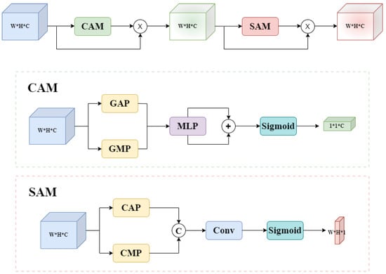
Figure 2.
Composition of the CBAM structure. Channel attention module (CAM) and spatial attention module (SAM), which incorporate operations such as global average pooling (GAP) and global max pooling (GMP) along the spatial dimensions. Channel average pooling (CAP) and channel max pooling (CMP) are performed along the channel dimensions.
2.4. Loss Functions
In object detection networks, object localization accuracy is typically assessed using IoU. However, in cases where there is no overlap between the two bounding boxes, IoU loss can lead to gradient vanishing, affecting the model’s effective updates. To address this issue, a series of improved loss functions have been introduced. Ref. [36] proposed ratio-balanced angle loss, enabling better balance between low and high-aspect ratio objects, avoiding redundant designs, and enhancing small object detection quality. Despite its effectiveness in handling small objects with varying aspect ratios, this method may be susceptible to background noise in complex environments, potentially increasing false detections. Ref. [37] introduced the concept of the minimum bounding box to alleviate the issue of gradient vanishing associated with IoU loss, enhancing training stability by providing a more accurate representation of object bounding boxes. Additionally, ref. [38] proposed incorporating a distance factor to accelerate model convergence, though it may have limitations in handling objects of varying scales. Furthermore, ref. [39] considered the aspect ratio associated with anchor boxes, leading to enhanced detection performance, particularly for objects with diverse aspect ratios. However, the presence of low-quality instances in the dataset unavoidably introduces significant discrepancies in both the distance and aspect ratios. These factors may excessively penalize poor-quality examples, diminishing the algorithm’s generalization capability. To overcome this challenge, we integrate the bounding box loss function proposed by [40] into our model. This approach effectively balances the treatment of instances with varying qualities, thereby improving the model’s robustness and generalization ability.
3. Methods
This section presents a detailed overview of our proposed method, FFEDet. We use YOLOv7, a well-known anchor-based one-stage detector, as the foundation for presenting our approach. It is important to emphasize that our method is not only applicable to YOLOv7 but also effectively utilized in both single-stage and two-stage detectors. In Section 3.1, we will revisit YOLOv7 to establish a foundation. Subsequently, Section 3.2 and Section 3.3 will delve into the structures of ECFA and SEConv. Section 3.4 will introduce the dynamic focus sample weighting function (DFSLoss), while the similarity measurement methods will be described in Section 3.5.
3.1. Revisiting YOLOv7
YOLOv7, which represents a progression in the YOLO series, has exhibited remarkable efficiency and precision in comparison to various object detection methods. The model mainly comprises three parts: a backbone to extract features, a neck structure to fuse these features, and a head structure to output the detection results. YOLOv7 incorporates several innovative technologies to enhance its performance, including an SPPCSPC module, reparameterized convolutions, efficient layer aggregation networks, and dynamic label assignment. Figure 3 illustrates the structure of the SPPCSPC module. First, the input feature map undergoes a 1 × 1 convolution operation (Conv1 × 1), followed by a 3 × 3 convolution operation (Conv3 × 3), and then another 1 × 1 convolution operation. These convolution operations generate intermediate feature maps. Next, these feature maps are processed through three max-pooling layers of different sizes (MP5 × 5, MP9 × 9, and MP13 × 13) for multi-scale pooling. The pooled feature maps are concatenated with the original feature map, creating a higher-dimensional feature map. This high-dimensional feature map then undergoes further processing with another series of 1 × 1, 3 × 3, and 1 × 1 convolution operations. Finally, the processed feature maps are concatenated again, producing the enhanced output feature map. In the realm of YOLOv7, including variants like YOLOv7-tiny and YOLOv7-X, our primary focus is on standard YOLOv7 as the reference model. We place special emphasis on the effectiveness and capability to operate in real time.

Figure 3.
Composition of the SPPCSPC structure. The SPPCSPC module processes the input feature map through multi-scale pooling and convolution operations to generate higher-dimensional features, followed by multiple convolutions and concatenations, ultimately outputting the enhanced feature map.
3.2. Efficient Cross-Scale Information Fusion Attention
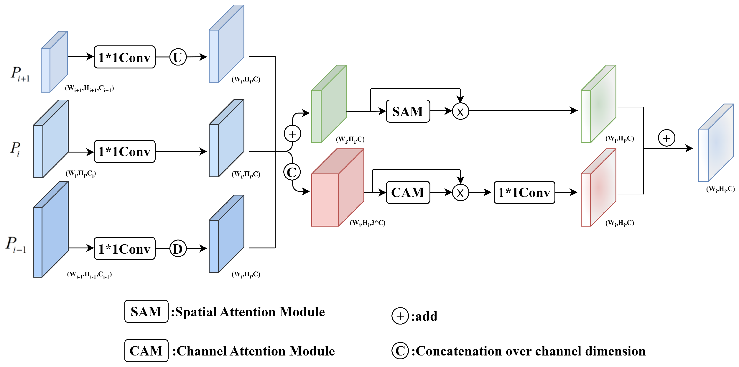
In object detection tasks, objects exhibit variations in size and shape across different scales. Consequently, cross-scale feature fusion plays a pivotal role in enhancing the understanding of objects within images and refining detection accuracy. By amalgamating features across different scales, the representational capacity of features is fortified, thereby fostering improved model generalization and robustness. Particularly noteworthy is the escalating depth of the model, exacerbating the challenge of fine-grained detail loss, especially pronounced in detecting small objects, thereby complicating the detection process. The efficient cross-scale information fusion attention (ECFA) module employs an efficient strategy for cross-scale feature fusion, effectively integrating multi-scale information through upsampling, downsampling, and concatenation of feature maps from different scales. This enables the model to dynamically adapt to the diverse scales inherent in object detection tasks. Attention mechanisms, initially successful in natural language processing, have now found broad application across various domains, including computer vision. These mechanisms aim to enhance model performance by guiding the model’s attention towards salient information, mitigating noise, and facilitating contextual modeling and information interaction across different scales of feature maps. Consequently, the ECFA module utilizes attention mechanisms for cross-scale feature fusion and interaction, in conjunction with SAM and CAM, to capture crucial spatial and channel information, thereby amplifying the model’s discriminative capability and accuracy. Figure 4 illustrates the structure of ECFA. Firstly, we independently apply convolutional layers to feature maps (, , ), (, , ), and (, , ) obtained from three adjacent scale levels. Subsequently, we perform downsampling and upsampling operations on and , resulting in three feature maps of equal shape: (, , C), (, , C), and (, , C). Next, we perform element-wise addition and channel-wise concatenation on these feature maps, obtaining feature maps of sizes (, , C) and (, , ). Then, we apply spatial attention and channel attention operations separately. Finally, we combine the results using weighted fusion to extract more comprehensive object information. This module enhances the representation capability for small objects by effectively focusing on different feature maps. The spatial and channel attention operations can be mathematically represented as follows:
where F represents the input feature. In the spatial attention operation, F undergoes channel-wise average and max pooling, then concatenation along the channel dimensions, and passes sequentially through the convolutional layer followed by the Sigmoid activation function, generating weight . Finally, the original feature F is multiplied by these weights to acquire the updated feature. Next, we apply the spatial average and max pooling to F during the channel attention operation. Then, the outcomes are individually passed through a two-layer neural network using ReLU activation. Parameters in this neural network are shared among its layers. Then, the two resulting features are summed, and the Sigmoid activation function is used to obtain the weights . Ultimately, the updated feature emerges from the multiplication of the weight with the initial feature F.
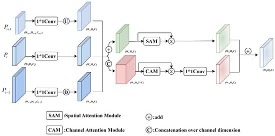
Figure 4.
Composition of the ECFA structure, which receives feature maps from three hierarchical scales, namely , , and . Downsampling and upsampling operations are applied to and . The resulting outcomes are then added to and concatenated, with spatial and channel attention mechanisms applied.
3.3. Simple and Efficient Convolution Module
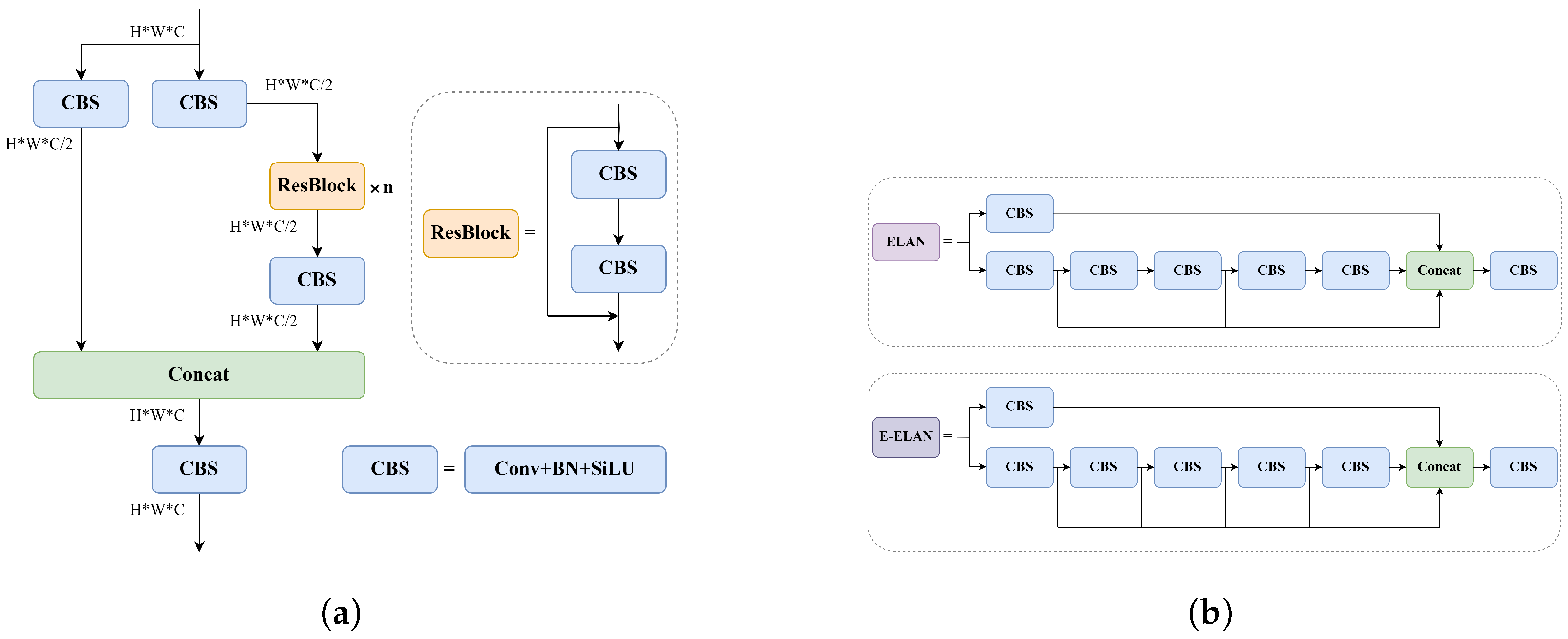
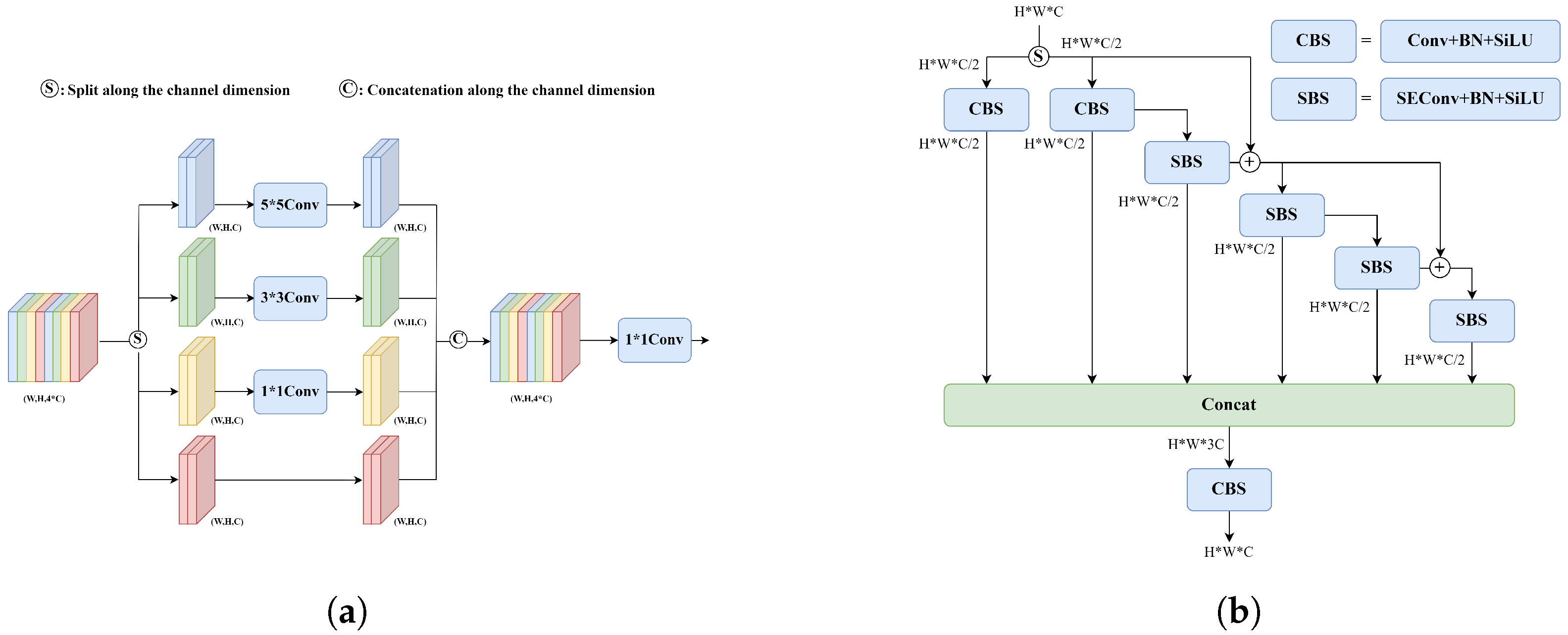
To enhance the feature learning capability of the model, ref. [41] introduced the CSP module, which can be integrated with the residual modules in ResNet to become a core structure in many mainstream detectors. Figure 5a provides a detailed illustration of the CSP module. The input undergoes two branches, with one employing a recurrent, residual structure for multiple iterations. Subsequently, the outputs from both branches are concatenated along the channel dimension. In ref. [2], ELAN and E-ELAN abandoned the dual-branch structure, as depicted in Figure 5b. In the ELAN module, feature fusion is achieved by integrating the output of each stacked module layer, while in the E-ELAN model, feature fusion is accomplished by incorporating the output of each convolutional layer within the stacked module. This allows the feature maps to gather information from multiple receptive fields, enhancing the model’s capability to extract features at various scales. However, standard 3 × 3 convolutional layers extract a significant portion of redundant features and introduce a considerable number of parameters and FLOPs. Therefore, we propose the simple and efficient convolution (SEConv) module, which reduces redundant computations, promotes the learning of representative features, and provides a multi-scale receptive field. The structure of SEConv is illustrated in Figure 6a. Experimental results in Table 1 demonstrate that SEConv exhibits notable advantages in terms of parameter count and computational complexity compared to standard 3 × 3 convolutional layers. We extend SEConv into the ELAN framework, proposing the S-ELAN module. As shown in Figure 6b, S-ELAN represents an enhanced version derived from the ELAN and E-ELAN structures. S-ELAN partitions the input feature map along the channel dimension into two equally shaped segments, each directed into separate branches. Subsequently, S-ELAN replaces the stacked standard convolution with the SEConv module proposed in this study. Finally, the resulting feature maps from each layer are concatenated along the channel dimension, and channel dependencies are extracted through a standard convolution with a 1 × 1 kernel size. The results in Table 5 illustrate that the S-ELAN module maintains excellent detection performance while simultaneously reducing the model’s computational complexity.
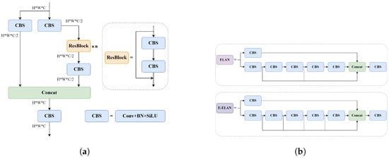
Figure 5.
The Structure of CSP, ELAN, and E-ELAN. (a) CSP: the input is passed through two branches. One of the branches employs a recurrent residual structure for multiple iterations. Then, the outputs are concentrated from both branches along the channel dimension. (b) ELAN and E-ELAN: in the ELAN module, feature fusion is accomplished by integrating the output of each stacked module layer, while in the E-ELAN model, feature fusion is achieved by incorporating the output of each convolutional layer within the stacked module.
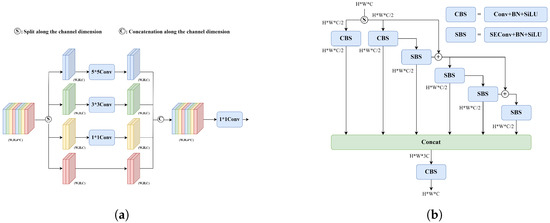
Figure 6.
The Structure of SEConv and S-ELAN. (a) SEConv: employing varied receptive field convolutions facilitates the extraction of multi-scale information, e.g., extracting inter-channel dependency information using pointwise convolutions. (b) S-ELAN: the input splits into two branches, employing stacked SEConv modules and residual fusion techniques.

Table 1.
Performance comparison between Conv and SEConv.
3.4. Dynamic Focal Sample Weighting Function
Regarding the IoU based on the prediction box to ground truth box, we categorize samples into two classes: easy and hard. Typically, easy samples have a more pronounced impact on the loss function, which can make it challenging for the model to effectively handle hard samples. To tackle this challenge, we devise an innovative, dynamic focal sample weighting function, referred to as DFSLoss.
which empowers the model to prioritize its attention on samples that are closer to the threshold boundaries, both normal and hard, by assigning higher weights to them during training. Consequently, the model has the capability to minimize the influence of simple samples in the model optimization process and more efficiently learn from normal and hard samples. To enhance the training stability of the model, we employ an exponential moving average (EMA) method to optimize IoU values between all bounding boxes, using their average as the threshold . Based on this threshold, samples are classified as negative (an IoU less than ) or positive (an IoU greater than ). However, due to the errors introduced by classification, samples near the threshold often suffer more substantial losses. Therefore, we aim for the model to more comprehensively learn from and optimize these samples near the threshold, leading to improved network training.
3.5. Similarity Measurement
In object detection, bounding box regression is the key to accurately locating objects. The IoU loss function ensures that prediction boxes closely align with the actual objects, ultimately leading to improved accuracy in object localization.
where A represents the prediction boxes, while B represents the ground truth boxes. YOLOv7 employs the CIoU loss function.
where is used to balance the different terms within the loss function, and quantifies the aspect ratio consistency with the anchor box.
where x, y, w, h, , , , and , respectively, denote the center coordinates and dimensions of the predicted box and the corresponding ground truth box. Moreover, and indicate the dimensions of the minimum anchor box that encompasses both the predicted box and the ground truth box. The CIoU loss function considers various factors, such as the center point distance or the width-to-height proportion of bounding boxes. However, training data may contain low-quality examples with issues like background noise, inconsistent aspect ratios, and other geometric factors. These issues can adversely affect the model’s training, especially when it comes to addressing geometric factors. To mitigate these problems, we introduce Wise-IoU [40], which helps to reduce the penalty for geometric factors when anchor boxes and object boxes have good overlap, thus reducing interference from training data.
where has the capability to magnify the IoU loss for common quality anchor boxes while reducing high-quality anchor boxes. When there is a lot of overlap between the bounding box and the object box, pays more attention to the distance between their centers. To prevent potential gradient issues introduced by , we separate and (indicated by ). This separation effectively eliminates factors that might hinder convergence without the need to introduce new metrics like aspect ratio. WIoUv2 constructs a monotonic focusing factor.
where represents an exponentially moving average with momentum utilized to address the problem of diminished convergence rate in the latter phases of model. We reflect anchor box quality by defining outliers, with high-quality anchor boxes having smaller outliers. By matching them with smaller gradient gains, it can effectively mitigate larger harmful gradients caused by low-quality samples. WIoUv3 introduces a non-linear focus factor, , to dynamically adjust the gradient amplification allocation strategy.
By allowing to be dynamic and accommodating different standards for evaluating the quality of anchor boxes, WIoUv3 is able to adapt to various anchor box quality assessment standards. This fine-tuning helps to reduce the detrimental impacts of varying anchor box quality during training.
4. Experiments
4.1. Implementation Details
In this study, we employed an NVIDIA RTX A6000 GPU for model training and implemented the algorithms using the PyTorch 1.8 framework. Training was conducted for 150 iterations on each dataset, with each iteration taking approximately 50 s, resulting in a total training time of roughly 2 h. For specific details regarding the experimental setup, please refer to Table 2.

Table 2.
Experimental environment.
We adopted YOLOv7 as our baseline model, configuring the input image size to 640 × 640, and employed SGD optimization with momentum. During the initial three iterations of training, the momentum value was set to 0.8 and subsequently adjusted to 0.937. The model was initialized with a learning rate of 0.01, which was decreased by a factor of 0.1 during the 50th and 100th iterations. To mitigate overfitting, we applied data augmentation techniques, including mosaic augmentation and random cropping, and incorporated a weight decay factor of 0.0005. Speed and accuracy tests were conducted with a batch size of 1. The IoU threshold for non-maximum suppression (NMS) was set to 0.5.
4.2. Datastes
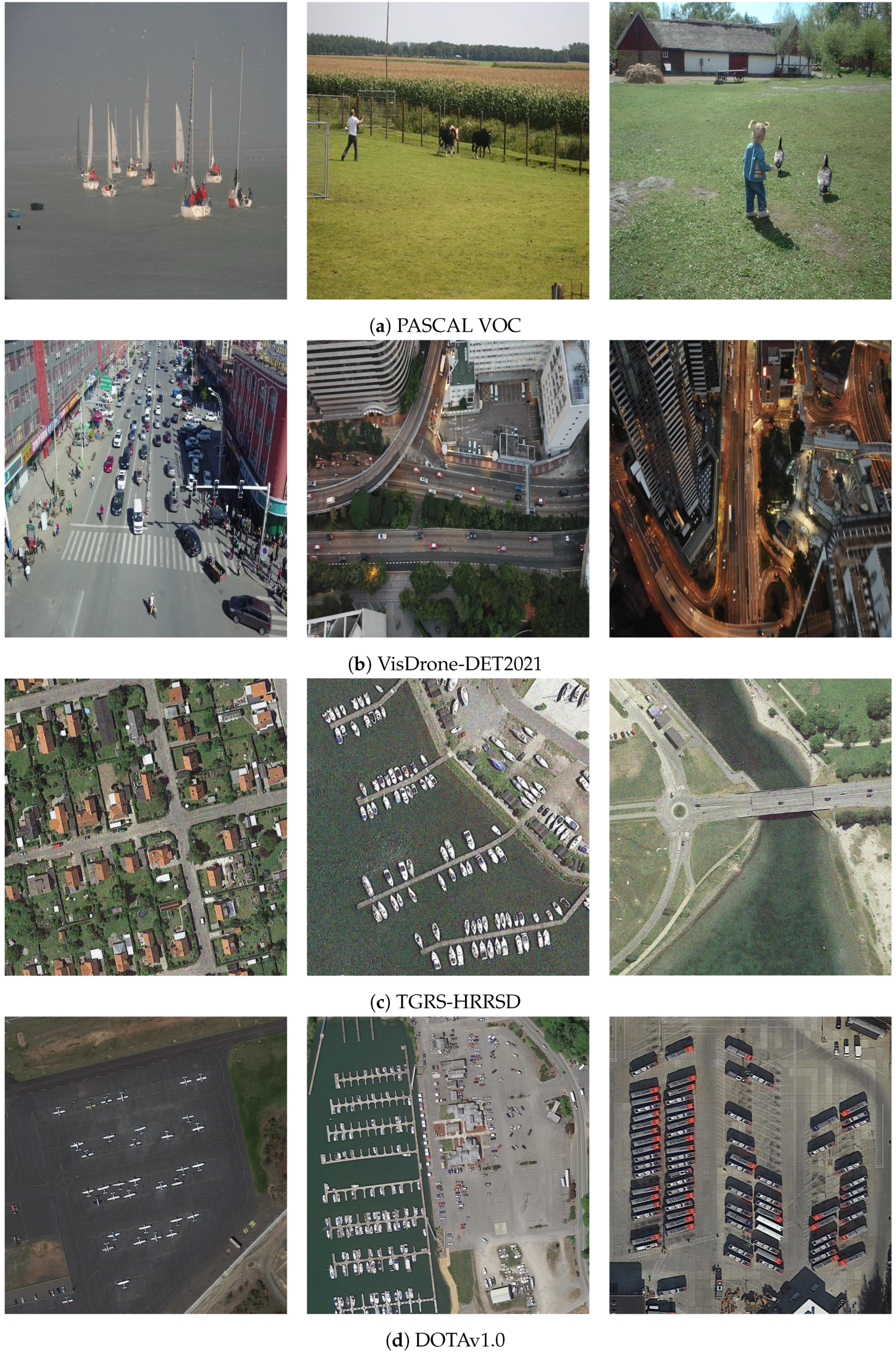
To evaluate the superiority of our suggested approach, four demanding public datasets were chosen for this paper: VisDrone-DET2021 [42], TGRS-HRRSD [43], DOTAv1.0 [44], and PASCAL VOC [45]. As shown in Figure 7, we showcase a selection of examples taken from these four public datasets. The choice of these datasets aimed to cover various application scenarios across different domains, providing a comprehensive evaluation of our method’s performance.
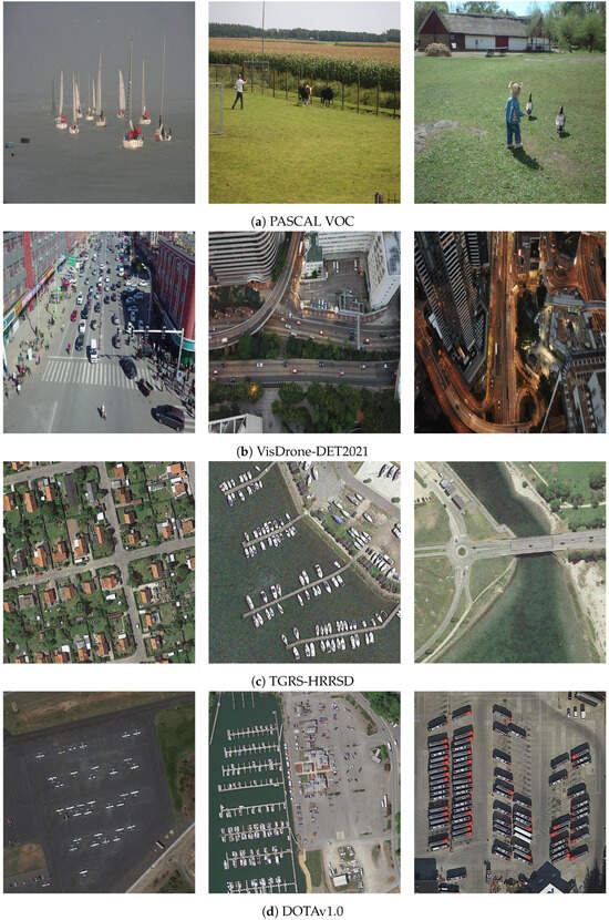
Figure 7.
The partial examples from the dataset, labeled from (a–d), correspond to PASCAL VOC, VisDrone-DET2021, TGRS-HRRSD, and DOTAv1.0, respectively.
VisDrone-DET2021 dataset: This dataset consists of 10,209 high-quality images with high resolution. It contains 10 different classes of objects with 6471 training, 548 validation, and 3190 testing images. The use of this dataset for evaluating the performance of small object detection models is challenging due to the noticeable imbalances in class distribution and object sizes.
TGRS-HRRSD dataset: This dataset comprises a comprehensive collection of21,761 images encompassing 13 classes of objects, totaling 55,740 object instances. Furthermore, the dataset is partitioned into 5401 training, 5417 validation, and 10,943 testing images. It was created by the Chinese Academy of Sciences in 2019. Image resolutions vary from 150 × 150 to 1200 × 1200, with average aspect ratios ranging from 41.96 to 276.50 pixels per category.
DOTAv1.0 dataset: The DOTAv1.0 dataset comprises aerial images that have been annotated using horizontal bounding boxes. It comprises 2806 images and encompasses 15 object categories. Due to the large original image resolutions, handling them directly can be challenging. A common practice is to crop each image into 640 × 640 patches with a 320-pixel stride, generating corresponding annotations for each cropped image. The processed dataset totals 21,046 images and 188,282 instances, and covers 15 object categories.
PASCAL VOC dataset: Recognized as a extensively utilized benchmark, the PASCAL VOC dataset holds significant importance for object detection tasks within the domain. For this study, we combined Pascal VOC 2007 and 2012 and obtained a consolidated dataset comprising 16,551 training images and 40,058 object objects, as well as 4952 validation images with 12,032 objects.
4.3. Evaluation Metrics
Average precision (AP) is a comprehensive performance measure frequently employed in the field of object detection, utilized to assess the detection capability for different classes. It relies on both precision and recall. Precision (P) can be formulated as follows:
Recall (R) can be defined as follows:
where TP, FP, and FN represent the true positive, false positive, and false negative, respectively. The formula for calculating the average precision (AP) can be written as follows:
where the mean average precision (mAP) at an IOU threshold of 0.5 is denoted as . The h within the IOU threshold range from 0.5 to 0.95, with an increment of 0.05, is referred to as . The mean average precision is defined as follows:
where and N denote the average precision and number of categories for category i. In addition, corresponds to the average precision for objects with an area smaller than . pertains to objects with an area ranging from to , while pertains to objects with an area larger than . FPS (frames per second) measures the detection speed of a model in terms of the number of recognizable frames per second and is widely used to evaluate the real-time capability of a model.
4.4. Result and Analysis
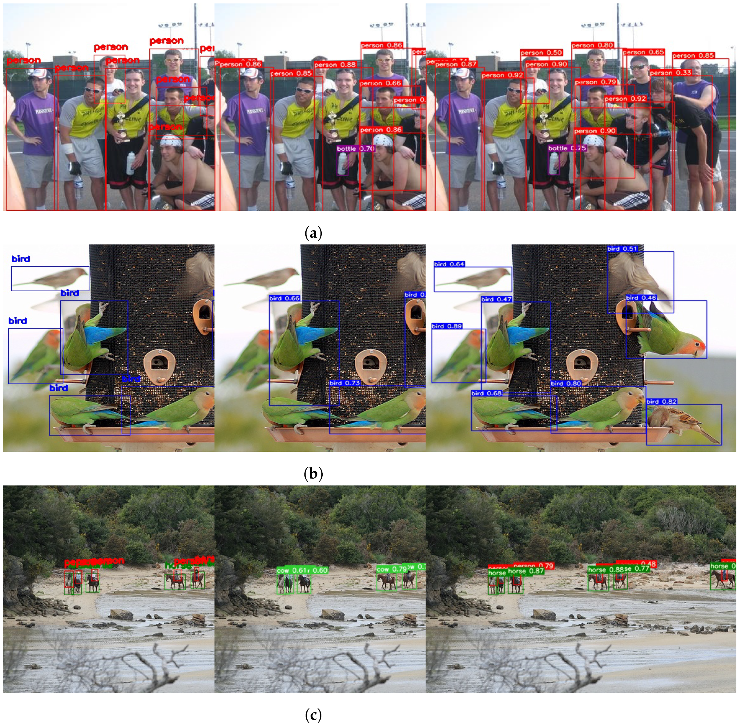
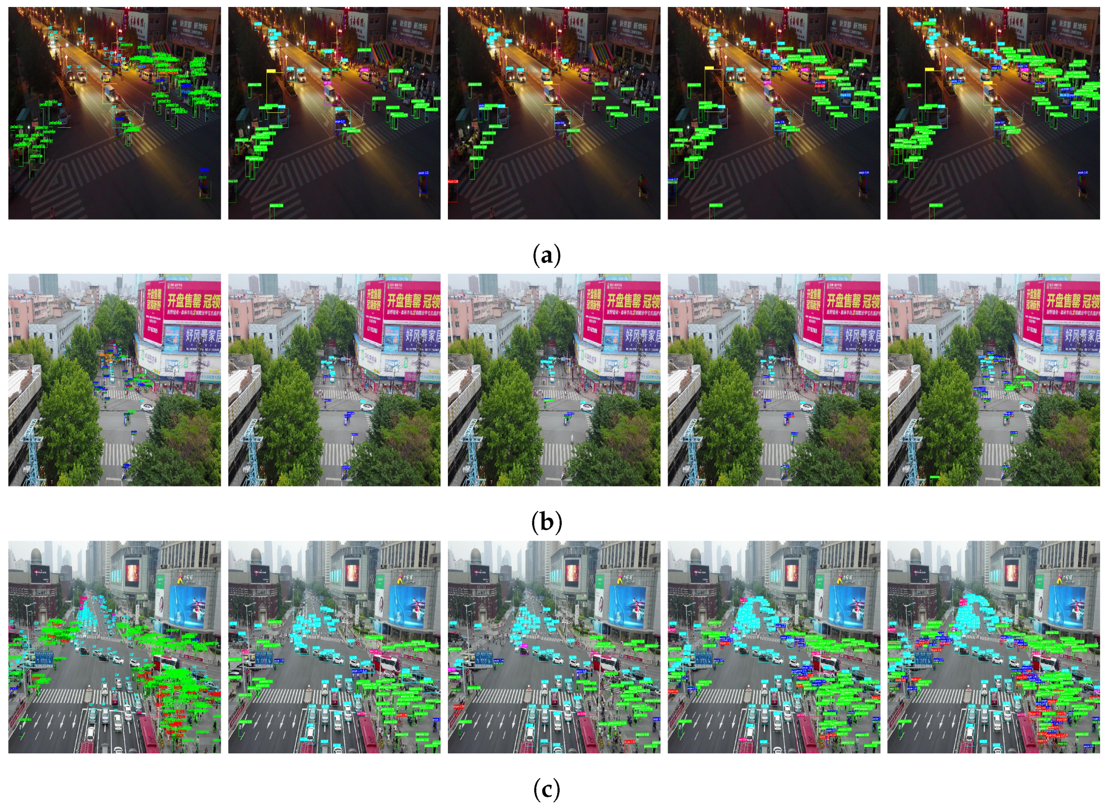
In this segment, a full analysis of our experimental findings will be presented. We selected mAP as our primary evaluation metric. The quantitative results are summarized in Table 3, and visual outcomes are showcased in Figure 8, Figure 9, Figure 10 and Figure 11.

Table 3.
Experimental results of different detection algorithms on the PASCAL VOC, VisDrone-DET2021, TGRS-HRRSD, and DOTAv1.0 datasets.
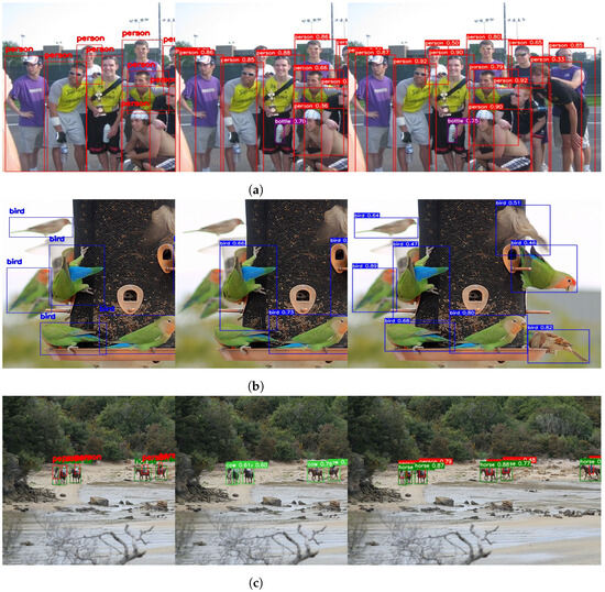
Figure 8.
Qualitative examples of small object scene detection on Pascal VOC. (a) Qualitative example of image 1. (b) Qualitative example of image 2. (c) Qualitative example of image 3. Each row displays, from left to right, the detection results consisting of the ground truth bounding boxes, the YOLOv7 algorithm, and our algorithm.
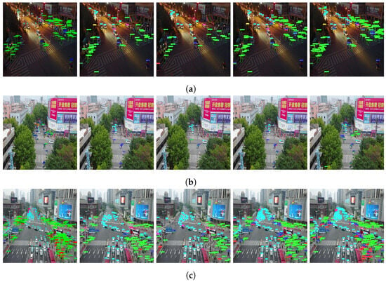
Figure 9.
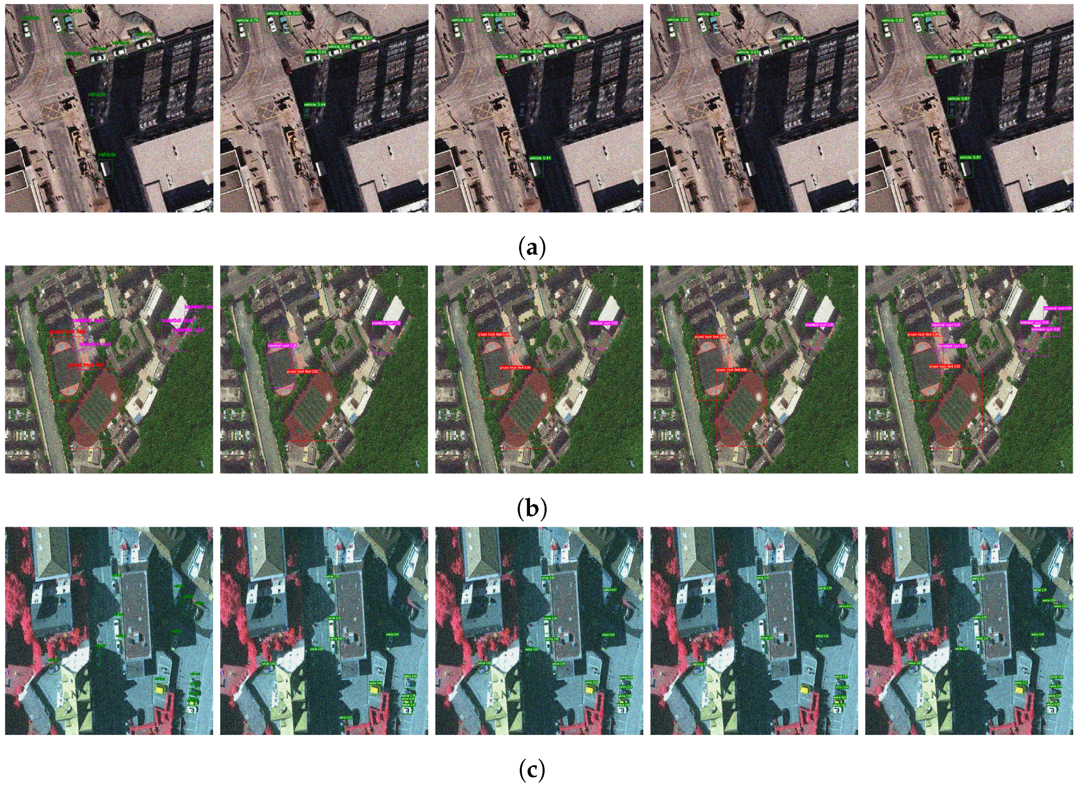
Qualitative examples of small object scene detection on VisDrone-DET2021. (a) Qualitative example of image 1. (b) Qualitative example of image 2. (c) Qualitative example of image 3. Each row displays, from left to right, the detection results consisting of the ground truth bounding boxes, the YOLOv5 algorithm, the YOLOv7 algorithm, the YOLOv8 algorithm, and our algorithm.
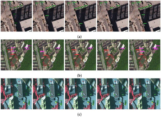
Figure 10.
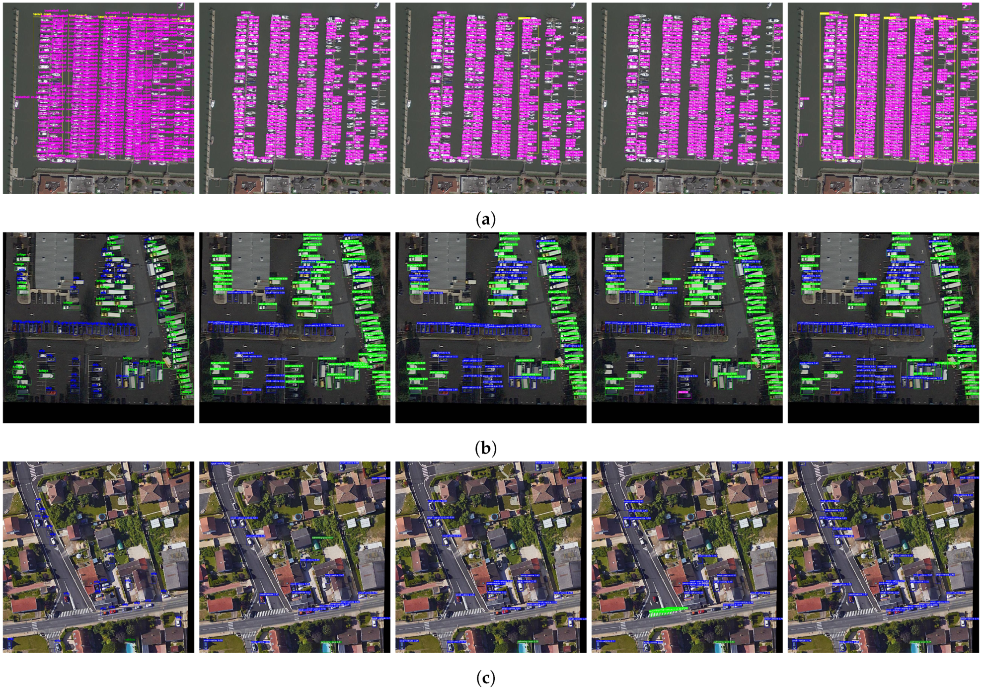
Qualitative examples of small object scene detection on TGRS-HRRSD. (a) Qualitative example of image 1. (b) Qualitative example of image 2. (c) Qualitative example of image 3. Each row displays, from left to right, the detection results consisting of the ground truth bounding boxes, the YOLOv5 algorithm, the YOLOv7 algorithm, the YOLOv8 algorithm, and our algorithm.
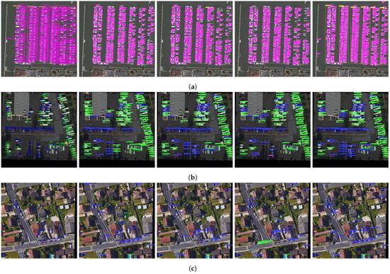
Figure 11.
Qualitative examples of small object scene detection on DOTAv1.0. (a) Qualitative example of image 1. (b) Qualitative example of image 2. (c) Qualitative example of image 3. Each row displays, from left to right, the detection results consisting of the ground truth bounding boxes, the YOLOv5 algorithm, the YOLOv7 algorithm, the YOLOv8 algorithm, and our algorithm.
The experimental results outlined in Table 3 delineate the performance metrics obtained by various detection algorithms across four distinct datasets (PASCAL VOC, VisDrone-DET2021, TGRS-HRRSD, and DOTAv1.0). For each dataset, performance parameters of the baseline method (Baseline), YOLOv5l, YOLOv8l, and our proposed method (Ours) are itemized, encompassing the model parameter count (Params(M)), average precision at varying IoU thresholds (, ), average precision across small, medium, and large objects (, , ), and frames per second processing speed (FPS).
Overall, our method (Ours) eclipsed other algorithms across all datasets. Notably, a substantial improvement was observed in the VisDrone-DET2021 dataset. Relative to the YOLOv7 baseline model, our method exhibited enhancements of 4.8% and 4.1% in and AP, respectively. Moreover, , , and experienced boosts of 4.5%, 3.8%, and 0.4%, correspondingly. The significant augmentation in APs underscores the efficacy of our method in detecting and classifying small objects. On the PASCAL VOC dataset, our method achieved improvements of 1.1%, 1.3%, and 1.1% in , AP, and , respectively; on the TGRS-HRRSD dataset, enhancements of 1.6%, 1.2%, and 2.3% were achieved; on the DOTAv1.0 dataset, enhancements of 1.5%, 1.5%, and 1.4% were observed. Our method consistently maintained optimal performance.
Despite not emerging as the top performer in FPS, our method still approached the optimal level. Although our model’s inference speed slightly lagged behind that of competing methods, it still satisfied the real-time detection requirement (i.e., processing over 60 frames per second). Hence, our method strikes a balance between performance and speed, furnishing a viable solution for practical applications. Furthermore, the standard deviation following each performance metric did not exceed 0.3, indicating the stability and reliability of the experimental results. These findings underscore the superiority of our method in object detection tasks and its promising prospects for application.
Furthermore, we present visualizations of the detection results from different algorithms applied to various datasets, as illustrated in Figure 8, Figure 9, Figure 10 and Figure 11. From top to bottom, examples of detections (a), (b), and (c) are presented. Each row displays the detection results from left to right, including the ground truth bounding boxes, the YOLO series algorithms, and our proposed algorithm. From these figures, it can be observed that YOLOv5, YOLOv7, and YOLOv8 are prone to missing and misclassifying small objects in scenes with complex backgrounds and dense occlusions. In contrast, our approach excels at accurately identifying small objects in complex situations, including occlusion, complex backgrounds, and densely populated object environments.
While the FFEDet model excels in object detection tasks, it may encounter limitations when dealing with highly cluttered scenes, necessitating improvements in its robustness. Additionally, enhancements in computational efficiency and generalization capabilities are required to accommodate diverse scenarios and datasets. Future research endeavors should focus on enhancing the model’s performance and applicability, thereby facilitating its widespread adoption in practical applications.
4.5. Ablation Study
To assess the contribution of each module to the model performance, we conducted ablation studies on the VisDrone-DET2021 dataset, with the baseline model being YOLOv7. The experimental results are shown in Table 4. The baseline (YOLOv7) achieved a of 49.1% and an AP of 28.0%. Each module (ECFA, SEConv, DFSLoss, and WIOUv3) exhibited improvements in performance compared to the baseline. Notably, the ECFA module significantly increased and AP by 2.9% and 2.6%, respectively. Subsequently, the SEConv module further enhanced and AP, with respective increments of 0.4% and 0.2%. Building upon this, the combination of the DFSLoss and WIOUv3 modules raised and AP to 53.9% and 32.1%, respectively, representing respective improvements of 4.8% and 4.1% over the baseline. These experimental results emphasize how each proposed module contributes to improving model performance, especially when considering the cumulative effects of ECFA, SEConv, DFSLoss, and WIOUv3. This further validates the efficacy of our approach in SOD tasks.

Table 4.
Ablation study on the VisDrone-DET2021 dataset.
To verify the superiority of SEConv, we conducted comparative experiments employing multiple widely used convolutional modules [46,47,48,49]. As shown in Table 5, PConv, DWConv, SCConv, and GSConv exhibited a decrease in parameters and computational complexity in comparison to the standard Conv layer, but their performance deteriorated. In contrast, our proposed SEConv achieved lower parameters and computational complexity than the standard Conv layer while demonstrating a noteworthy 0.6% improvement in .

Table 5.
A comparison of the performance of various convolution methods on the VisDrone-DET2021 dataset.
Table 5.
A comparison of the performance of various convolution methods on the VisDrone-DET2021 dataset.
| Method | Params(M) | FLOPs | AP | |
|---|---|---|---|---|
| Conv(Baseline) | 37.62 | 106.5 | 49.1 | 28.0 |
| DWConv | 34.12 | 98.3 | 48.9 | 27.4 |
| SCConv | 35.36 | 99.9 | 48.4 | 26.8 |
| PConv | 30.52 | 80.3 | 48.5 | 27.3 |
| GSConv | 29.54 | 77.1 | 48.1 | 26.9 |
| SEConv(Ours) | 35.84 | 102.8 | 49.7 | 28.2 |
To demonstrate the effectiveness of combining DFSLoss with Wise-IoU (WIoU), we selected the popular bounding box regression (BBR) loss for comparative experiments. As shown in Table 6, it can be observed that among various BBR loss functions, the performance achieved by DFSLoss and WIoUv3 consistently outperformed other models.

Table 6.
Performance comparison of DFSLoss combined with each bounding box loss on VisDrone-DET2021.
4.6. Comparative Experiments
We conducted a comparative analysis of our method with other state-of-the-art detectors on the VisDrone-DET2021 dataset. According to the information provided in Table 7, our approach demonstrated significant advantages in performance. Firstly, our model achieved the highest levels of , AP, and , reaching 53.9, 32.1, and 32.7, respectively. Compared to other methods, our approach showed a remarkable improvement in object detection accuracy. It is worth noting that HRDNet [53], queryDet [19], and ScaleKD [54] are advanced detectors specifically designed for small object detection. In contrast, our method achieved the best detection performance with relatively fewer parameters (39.52 M). This indicates that our method maintained model simplicity and efficiency while enhancing detection performance. Additionally, our method also demonstrated outstanding performance in inference speed, achieving a speed of 72.7 frames per second. This suggests that our model excels not only in detection accuracy but also in real-time applicability and efficiency. In summary, our method achieved significant performance improvement in small-object detection tasks, exhibiting higher detection accuracy, fewer parameters, and faster inference speed, demonstrating clear superiority.

Table 7.
Comparison results with other state-of-the-art methods on the VisDrone-DET2021 dataset.
5. Conclusions
In this study, we proposed FFEDet. Particularly, we proposed ECFA, an effective attention module for cross-scale feature aggregation, which effectively integrates feature information from various scales, emphasizes relevant features, suppresses irrelevant noise, and enhances feature representation. Additionally, we proposed SEConv, a simple and efficient convolutional module that reduces computational complexity and expands the receptive field across multiple scales. Furthermore, we proposed DFSLoss, which is a dynamic focus sample weighting function that assigns greater weights to normal and challenging samples, thus addressing the imbalance in the distribution of easy and hard samples. Moreover, we introduced Wise-IoU to alleviate the detrimental impact of low-quality examples on model convergence. The outcomes of the experiments conducted on four public datasets evidently demonstrate the outstanding performance of FFEDet. For future research, we aim to explore more lightweight model design options to enhance the model’s inference speed while preserving high accuracy. This may entail utilizing more compact network architectures, introducing more effective parameter-sharing strategies, or adopting more flexible attention mechanisms. Additionally, we will further investigate data augmentation techniques and explore more diverse and refined sample selection methods to bolster the model’s generalization ability and robustness. Moreover, we intend to explore the potential applications of the FFEDet model in various domains and tasks. For instance, we plan to deploy it in fields such as medical image analysis and intelligent surveillance systems to validate its adaptability and versatility across diverse scenarios. This exploration will offer us additional opportunities to refine the model and assess its performance in real-world applications.
Author Contributions
Conceptualization, F.Z. and J.Z.; methodology, F.Z.; software, F.Z.; validation, F.Z.; formal analysis, F.Z.; investigation, F.Z.; resources, F.Z. and G.Z.; data curation, F.Z.; writing—original draft preparation, F.Z. and G.Z.; writing—review and editing, F.Z.; visualization, F.Z.; supervision, F.Z.; project administration, F.Z. and J.Z.; funding acquisition, J.Z. All authors have read and agreed to the published version of the manuscript.
Funding
This research was supported by the National Natural Science Foundation of China (No. 62076137).
Data Availability Statement
The raw data supporting the conclusions of this article will be made available by the authors on request.
Conflicts of Interest
The authors declare no conflicts of interest.
References
- Cheng, G.; Yuan, X.; Yao, X.; Yan, K.; Zeng, Q.; Xie, X.; Han, J. Towards large-scale small object detection: Survey and benchmarks. IEEE Trans. Pattern Anal. Mach. Intell. 2023, 45, 13467–13488. [Google Scholar] [CrossRef]
- Wang, C.Y.; Bochkovskiy, A.; Liao, H.Y.M. YOLOv7: Trainable bag-of-freebies sets new state-of-the-art for real-time object detectors. In Proceedings of the IEEE/CVF Conference on Computer Vision and Pattern Recognition, Vancouver, BC, Canada, 18–22 June 2023; pp. 7464–7475. [Google Scholar]
- Zhang, G.; Luo, Z.; Chen, Y.; Zheng, Y.; Lin, W. Illumination unification for person re-identification. IEEE Trans. Circuits Syst. Video Technol. 2022, 32, 6766–6777. [Google Scholar] [CrossRef]
- Karen, S. Very deep convolutional networks for large-scale image recognition. arXiv 2014, arXiv:1409.1556. [Google Scholar]
- Redmon, J.; Farhadi, A. Yolov3: An incremental improvement. arXiv 2018, arXiv:1804.02767. [Google Scholar]
- Zhang, G.; Fang, W.; Zheng, Y.; Wang, R. A Spatial Dual-Branch Attention Dehazing Network based on Meta-Former Paradigm. IEEE Trans. Circuits Syst. Video Technol. 2023, 34, 60–70. [Google Scholar] [CrossRef]
- Gao, S.; Cheng, M.; Zhao, K.; Zhang, X.; Yang, M.; Torr, P. Res2Net: A New Multi-Scale Backbone Architecture. IEEE Trans. Pattern Anal. Mach. Intell. 2021, 43, 652–662. [Google Scholar] [CrossRef]
- Zhang, G.; Zhang, H.; Lin, W.; Chandran, A.K.; Jing, X. Camera contrast learning for unsupervised person re-identification. IEEE Trans. Circuits Syst. Video Technol. 2023, 4096–4107. [Google Scholar] [CrossRef]
- He, K.; Zhang, X.; Ren, S.; Sun, J. Spatial pyramid pooling in deep convolutional networks for visual recognition. IEEE Trans. Pattern Anal. Mach. Intell. 2015, 37, 1904–1916. [Google Scholar] [CrossRef]
- Faster, R. Towards real-time object detection with region proposal networks. Adv. Neural Inf. Process. Syst. 2015, 9199, 2969239–2969250. [Google Scholar]
- Zhang, G.; Liu, J.; Chen, Y.; Zheng, Y.; Zhang, H. Multi-biometric unified network for cloth-changing person re-identification. IEEE Trans. Image Process. 2023, 32, 4555–4566. [Google Scholar] [CrossRef]
- Liu, W.; Anguelov, D.; Erhan, D.; Szegedy, C.; Reed, S.; Fu, C.Y.; Berg, A.C. Ssd: Single shot multibox detector. In Proceedings of the Computer Vision–ECCV 2016: 14th European Conference, Amsterdam, The Netherlands, 11–14 October 2016; Proceedings, Part I 14. Springer: Berlin/Heidelberg, Germany, 2016; pp. 21–37. [Google Scholar]
- Fu, C.Y.; Liu, W.; Ranga, A.; Tyagi, A.; Berg, A.C. Dssd: Deconvolutional single shot detector. arXiv 2017, arXiv:1701.06659. [Google Scholar]
- Redmon, J.; Farhadi, A. YOLO9000: Better, faster, stronger. In Proceedings of the IEEE Conference on Computer Vision and Pattern Recognition, Honolulu, HI, USA, 21–26 July 2017; pp. 7263–7271. [Google Scholar]
- Ge, Z.; Liu, S.; Wang, F.; Li, Z.; Sun, J. Yolox: Exceeding yolo series in 2021. arXiv 2021, arXiv:2107.08430. [Google Scholar]
- Bochkovskiy, A.; Wang, C.Y.; Liao, H.Y.M. Yolov4: Optimal speed and accuracy of object detection. arXiv 2020, arXiv:2004.10934. [Google Scholar]
- Ultralytics. ultralytics/yolov5: v7.0 - YOLOv5 SOTA Realtime Instance Segmentation. 2022. Available online: https://github.com/ultralytics/yolov5.com (accessed on 7 May 2023).
- Li, C.; Li, L.; Jiang, H.; Weng, K.; Geng, Y.; Li, L.; Ke, Z.; Li, Q.; Cheng, M.; Nie, W.; et al. YOLOv6: A single-stage object detection framework for industrial applications. arXiv 2022, arXiv:2209.02976. [Google Scholar]
- Yang, C.; Huang, Z.; Wang, N. Querydet: Cascaded sparse query for accelerating high-resolution small object detection. In Proceedings of the IEEE/CVF Conference on Computer Vision and Pattern Recognition, New Orleans, LA, USA, 18–24 June 2022; pp. 13668–13677. [Google Scholar]
- Aibibu, T.; Lan, J.; Zeng, Y.; Lu, W.; Gu, N. An efficient rep-style gaussian–wasserstein network: Improved uav infrared small object detection for urban road surveillance and safety. Remote Sens. 2023, 16, 25. [Google Scholar] [CrossRef]
- Yang, X.; Yang, J.; Yan, J.; Zhang, Y.; Zhang, T.; Guo, Z.; Sun, X.; Fu, K. Scrdet: Towards more robust detection for small, cluttered and rotated objects. In Proceedings of the IEEE/CVF International Conference on Computer Vision, Seoul, Republic of Korea, 27 October–2 November 2019; pp. 8232–8241. [Google Scholar]
- Xu, C.; Wang, J.; Yang, W.; Yu, L. Dot distance for tiny object detection in aerial images. In Proceedings of the IEEE/CVF conference on computer vision and pattern recognition, Nashville, TN, USA, 19–25 June 2021; pp. 1192–1201. [Google Scholar]
- Wang, J.; Xu, C.; Yang, W.; Yu, L. A normalized Gaussian Wasserstein distance for tiny object detection. arXiv 2021, arXiv:2110.13389. [Google Scholar]
- Shi, T.; Gong, J.; Hu, J.; Zhi, X.; Zhang, W.; Zhang, Y.; Zhang, P.; Bao, G. Feature-enhanced CenterNet for small object detection in remote sensing images. Remote Sens. 2022, 14, 5488. [Google Scholar] [CrossRef]
- Kong, T.; Yao, A.; Chen, Y.; Sun, F. Hypernet: Towards accurate region proposal generation and joint object detection. In Proceedings of the IEEE Conference on Computer Vision and Pattern Recognition, Las Vegas, NV, USA, 27–30 June 2016; pp. 845–853. [Google Scholar]
- Yang, F.; Choi, W.; Lin, Y. Exploit all the layers: Fast and accurate cnn object detector with scale dependent pooling and cascaded rejection classifiers. In Proceedings of the IEEE Conference on Computer Vision and Pattern Recognition, Las Vegas, NV, USA, 27–30 June 2016; pp. 2129–2137. [Google Scholar]
- Cai, Z.; Fan, Q.; Feris, R.S.; Vasconcelos, N. A unified multi-scale deep convolutional neural network for fast object detection. In Proceedings of the Computer Vision–ECCV 2016: 14th European Conference, Amsterdam, The Netherlands, 11–14 October 2016; Proceedings, Part IV 14. Springer: Berlin/Heidelberg, Germany, 2016; pp. 354–370. [Google Scholar]
- Liu, S.; Qi, L.; Qin, H.; Shi, J.; Jia, J. Path aggregation network for instance segmentation. In Proceedings of the IEEE Conference on Computer Vision and Pattern Recognition, Salt Lake City, UT, USA, 18–22 June 2018; pp. 8759–8768. [Google Scholar]
- Zhang, H.; Wang, K.; Tian, Y.; Gou, C.; Wang, F.Y. MFR-CNN: Incorporating multi-scale features and global information for traffic object detection. IEEE Trans. Veh. Technol. 2018, 67, 8019–8030. [Google Scholar] [CrossRef]
- Lin, T.Y.; Dollár, P.; Girshick, R.; He, K.; Hariharan, B.; Belongie, S. Feature pyramid networks for object detection. In Proceedings of the IEEE Conference on Computer Vision and Pattern Recognition, Honolulu, HI, USA, 21–26 July 2017; pp. 2117–2125. [Google Scholar]
- Li, Y.; Zhang, X.; Chen, D. Csrnet: Dilated convolutional neural networks for understanding the highly congested scenes. In Proceedings of the IEEE Conference on Computer Vision and Pattern Recognition, Salt Lake City, UT, USA, 18–22 June 2018; pp. 1091–1100. [Google Scholar]
- Liang, X.; Zhang, J.; Zhuo, L.; Li, Y.; Tian, Q. Small object detection in unmanned aerial vehicle images using feature fusion and scaling-based single shot detector with spatial context analysis. IEEE Trans. Circuits Syst. Video Technol. 2019, 30, 1758–1770. [Google Scholar] [CrossRef]
- Hu, J.; Shen, L.; Sun, G. Squeeze-and-excitation networks. In Proceedings of the IEEE Conference on Computer Vision and Pattern Recognition, Salt Lake City, UT, USA, 18–22 June 2018; pp. 7132–7141. [Google Scholar]
- Woo, S.; Park, J.; Lee, J.Y.; Kweon, I.S. Cbam: Convolutional block attention module. In Proceedings of the European Conference on Computer Vision (ECCV), Munich, Germany, 8–14 September 2018; pp. 3–19. [Google Scholar]
- Hou, Q.; Zhou, D.; Feng, J. Coordinate attention for efficient mobile network design. In Proceedings of the IEEE/CVF Conference on Computer Vision and Pattern Recognition, Nashville, TN, USA, 19–25 June 2021; pp. 13713–13722. [Google Scholar]
- Wang, M.; Li, Q.; Gu, Y.; Pan, J. Highly Efficient Anchor-Free Oriented Small Object Detection for Remote Sensing Images via Periodic Pseudo-Domain. Remote Sens. 2023, 15, 3854. [Google Scholar] [CrossRef]
- Rezatofighi, H.; Tsoi, N.; Gwak, J.; Sadeghian, A.; Reid, I.; Savarese, S. Generalized intersection over union: A metric and a loss for bounding box regression. In Proceedings of the IEEE/CVF Conference on Computer Vision and Pattern Recognition, Long Beach, CA, USA, 16–20 June 2019; pp. 658–666. [Google Scholar]
- Zheng, Z.; Wang, P.; Liu, W.; Li, J.; Ye, R.; Ren, D. Distance-IoU loss: Faster and better learning for bounding box regression. In Proceedings of the AAAI Conference on Artificial Intelligence, New York, NY, USA, 7–12 February 2020; Volume 34, pp. 12993–13000. [Google Scholar]
- Zheng, Z.; Wang, P.; Ren, D.; Liu, W.; Ye, R.; Hu, Q.; Zuo, W. Enhancing geometric factors in model learning and inference for object detection and instance segmentation. IEEE Trans. Cybern. 2021, 52, 8574–8586. [Google Scholar] [CrossRef]
- Tong, Z.; Chen, Y.; Xu, Z.; Yu, R. Wise-IoU: Bounding box regression loss with dynamic focusing mechanism. arXiv 2023, arXiv:2301.10051. [Google Scholar]
- Wang, C.Y.; Liao, H.Y.M.; Wu, Y.H.; Chen, P.Y.; Hsieh, J.W.; Yeh, I.H. CSPNet: A new backbone that can enhance learning capability of CNN. In Proceedings of the IEEE/CVF Conference on Computer Vision and Pattern Recognition Workshops, Seattle, WA, USA, 14–19 June 2020; pp. 390–391. [Google Scholar]
- Cao, Y.; He, Z.; Wang, L.; Wang, W.; Yuan, Y.; Zhang, D.; Zhang, J.; Zhu, P.; Van Gool, L.; Han, J.; et al. VisDrone-DET2021: The vision meets drone object detection challenge results. In Proceedings of the IEEE/CVF International Conference on Computer Vision, Montreal, BC, Canada, 11–17 October 2021; pp. 2847–2854. [Google Scholar]
- Zhang, Y.; Yuan, Y.; Feng, Y.; Lu, X. Hierarchical and robust convolutional neural network for very high-resolution remote sensing object detection. IEEE Trans. Geosci. Remote Sens. 2019, 57, 5535–5548. [Google Scholar] [CrossRef]
- Xia, G.S.; Bai, X.; Ding, J.; Zhu, Z.; Belongie, S.; Luo, J.; Datcu, M.; Pelillo, M.; Zhang, L. DOTA: A large-scale dataset for object detection in aerial images. In Proceedings of the IEEE Conference on Computer Vision and Pattern Recognition, Salt Lake City, UT, USA, 18–22 June 2018; pp. 3974–3983. [Google Scholar]
- Everingham, M.; Van Gool, L.; Williams, C.K.; Winn, J.; Zisserman, A. The pascal visual object classes (voc) challenge. Int. J. Comput. Vis. 2010, 88, 303–338. [Google Scholar] [CrossRef]
- Chollet, F. Xception: Deep learning with depthwise separable convolutions. In Proceedings of the IEEE Conference on Computer Vision and Pattern Recognition, Honolulu, HI, USA, 21–26 July 2017; pp. 1251–1258. [Google Scholar]
- Li, J.; Wen, Y.; He, L. Scconv: Spatial and channel reconstruction convolution for feature redundancy. In Proceedings of the IEEE/CVF Conference on Computer Vision and Pattern Recognition, Vancouver, BC, Canada, 17–24 June 2023; pp. 6153–6162. [Google Scholar]
- Chen, J.; Kao, S.h.; He, H.; Zhuo, W.; Wen, S.; Lee, C.H.; Chan, S.H.G. Run, Don’t walk: Chasing higher FLOPS for faster neural networks. In Proceedings of the IEEE/CVF Conference on Computer Vision and Pattern Recognition, Vancouver, BC, Canada, 17–24 June 2023; pp. 12021–12031. [Google Scholar]
- Li, H.; Li, J.; Wei, H.; Liu, Z.; Zhan, Z.; Ren, Q. Slim-neck by GSConv: A better design paradigm of detector architectures for autonomous vehicles. arXiv 2022, arXiv:2206.02424. [Google Scholar]
- Gevorgyan, Z. SIoU loss: More powerful learning for bounding box regression. arXiv 2022, arXiv:2205.12740. [Google Scholar]
- Zhang, Y.F.; Ren, W.; Zhang, Z.; Jia, Z.; Wang, L.; Tan, T. Focal and efficient IOU loss for accurate bounding box regression. Neurocomputing 2022, 506, 146–157. [Google Scholar] [CrossRef]
- Siliang, M.; Yong, X. Mpdiou: A loss for efficient and accurate bounding box regression. arXiv 2023, arXiv:2307.07662. [Google Scholar]
- Liu, Z.; Gao, G.; Sun, L.; Fang, Z. HRDNet: High-resolution detection network for small objects. In Proceedings of the 2021 IEEE International Conference on Multimedia and Expo (ICME), Shenzhen, China, 5–9 July 2021; IEEE: New York, NY, USA, 2021; pp. 1–6. [Google Scholar]
- Zhu, Y.; Zhou, Q.; Liu, N.; Xu, Z.; Ou, Z.; Mou, X.; Tang, J. Scalekd: Distilling scale-aware knowledge in small object detector. In Proceedings of the IEEE/CVF Conference on Computer Vision and Pattern Recognition, Vancouver, BC, Canada, 17–24 June 2023; pp. 19723–19733. [Google Scholar]
- Ultralytics. YOLO by Ultralytics (Version 8.0.0). 2023. Available online: https://github.com/ultralytics/ultralytics (accessed on 17 April 2023).
- Ozpoyraz, B.; Dogukan, A.T.; Gevez, Y.; Altun, U.; Basar, E. Deep learning-aided 6G wireless networks: A comprehensive survey of revolutionary PHY architectures. IEEE Open J. Commun. Soc. 2022, 3, 1749–1809. [Google Scholar] [CrossRef]
- Lin, T.Y.; Goyal, P.; Girshick, R.; He, K.; Dollár, P. Focal loss for dense object detection. In Proceedings of the IEEE International Conference on Computer Vision, Venice, Italy, 22–29 October 2017; pp. 2980–2988. [Google Scholar]
- Li, X.; Wang, W.; Hu, X.; Li, J.; Tang, J.; Yang, J. Generalized focal loss v2: Learning reliable localization quality estimation for dense object detection. In Proceedings of the IEEE/CVF Conference on Computer Vision and Pattern Recognition, Nashville, TN, USA, 19–25 June 2021; pp. 11632–11641. [Google Scholar]
- Xu, C.; Wang, J.; Yang, W.; Yu, H.; Yu, L.; Xia, G.S. RFLA: Gaussian receptive field based label assignment for tiny object detection. In Proceedings of the European Conference on Computer Vision, Tel Aviv, Israel, 23–27 October 2022; Springer: Berlin/Heidelberg, Germany, 2022; pp. 526–543. [Google Scholar]
Disclaimer/Publisher’s Note: The statements, opinions and data contained in all publications are solely those of the individual author(s) and contributor(s) and not of MDPI and/or the editor(s). MDPI and/or the editor(s) disclaim responsibility for any injury to people or property resulting from any ideas, methods, instructions or products referred to in the content. |
© 2024 by the authors. Licensee MDPI, Basel, Switzerland. This article is an open access article distributed under the terms and conditions of the Creative Commons Attribution (CC BY) license (https://creativecommons.org/licenses/by/4.0/).

