Deep-Learning-Based Daytime COT Retrieval and Prediction Method Using FY4A AGRI Data

Abstract

The traditional method for retrieving cloud optical thickness (COT) is carried out through a Look-Up Table (LUT). Researchers must make a series of idealized assumptions and conduct extensive observations and record features in this scenario, consuming considerable resources. The emergence of deep learning effectively addresses the shortcomings of the traditional approach. In this paper, we first propose a daytime (SOZA < 70°) COT retrieval algorithm based on FY-4A AGRI. We establish and train a Convolutional Neural Network (CNN) model for COT retrieval, CM4CR, with the CALIPSO’s COT product spatially and temporally synchronized as the ground truth. Then, a deep learning method extended from video prediction models is adopted to predict COT values based on the retrieval results obtained from CM4CR. The COT prediction model (CPM) consists of an encoder, a predictor, and a decoder. On this basis, we further incorporated a time embedding module to enhance the model’s ability to learn from irregular time intervals in the input COT sequence. During the training phase, we employed Charbonnier Loss and Edge Loss to enhance the model’s capability to represent COT details. Experiments indicate that our CM4CR outperforms existing COT retrieval methods, with predictions showing better performance across several metrics than other benchmark prediction models. Additionally, this paper also investigates the impact of different lengths of COT input sequences and the time intervals between adjacent frames of COT on prediction performance.

1. Introduction

Cloud optical thickness (COT) refers to the total attenuation produced by all absorbing and scattering substances per unit cross-section along the radiation transmission path, used to describe the degree of light attenuation when passing through a medium. COT affects the transparency of clouds, reflecting their extinction effect, and plays an important role in calculating cloud thickness. Additionally, cloud optical thickness strongly influences the radiative properties of clouds, such as the Greenhouse-versus-albedo effect of cirrus clouds, which mainly depends on the optical thickness (COT) [1,2]. Roeckner et al. [3] and Mitchel et al. [4] utilized General Circulation Model (GCM) simulations to investigate the impact of changes in liquid water content and optical thickness in clouds on climate, indicating that the negative feedback effect of changes in cloud optical properties is comparable to the positive feedback effect of changes in cloud amount. However, there is still insufficient understanding of cloud properties. The uncertainties in the interaction between clouds and radiation largely affect the accuracy of climate change predictions and numerical weather forecasts [5]. Therefore, obtaining accurate quantitative information about cloud microphysical parameters such as COT helps improve the accuracy of radiation characteristic calculations, thus enabling more precise weather forecasting [6]. Currently, the retrieval of cloud optical thickness (COT) has been widely studied. Accurate COT retrieval serves as a prerequisite for COT prediction. However, the accuracy of COT retrieval still needs improvement, resulting in limited research on COT prediction. To address the gap, we developed a more accurate and scientific COT retrieval algorithm and predicted COT using a time-series prediction model.

With the rapid development of deep learning, meteorological forecasting and applications have gradually become popular research directions under the impact of deep learning. Previous studies on meteorological information prediction, such as rainfall prediction [7], typhoon prediction [8], and satellite cloud image prediction [9], have achieved significant research results. Our research found that COT prediction is also a spatiotemporal sequence prediction problem. The main task of spatiotemporal sequence prediction is to use past temporal sequences of spatial data as input to predict future sequences for several time steps and output the prediction results. There is a strong desire for high-quality COT sequences for predicting COT. FY-4A, China’s new geostationary satellite, currently does not provide cloud optical thickness products. However, its multi-channel products ensure the acquisition of high-quality COT sequences. Therefore, the research route of this paper is to retrieve the value of daytime COT based on the dataset provided by FY-4A and predict the information of future COT based on the COT values we retrieved.

With the advancement of satellite technology, satellite observations provide substantial support for obtaining cloud parameters and their spatiotemporal variations at regional and global scales. In recent years, research utilizing satellite observations to retrieve cloud microphysical parameters has received increasing attention [10,11,12,13,14,15,16]. The fundamental principle of satellite-based COT retrieval is that in the visible light spectrum, cloud reflectance primarily depends on the value of COT [17]. Passive satellite observations, with the characteristics of long historical records, high temporal resolution and ample spatial coverage, have become one of the primary means to monitor cloud optical thickness at different spatiotemporal scales [15]. Over the past few decades, significant progress has been made in retrieving cloud optical thickness products from satellites. The MODIS sensors onboard Terra and Aqua have long monitored and released datasets of cloud optical thickness [18]. However, due to the time-sensitivity of cloud changes, polar-orbiting satellites cannot meet monitoring requirements well. Geostationary satellites, characterized by continuous monitoring, such as Himawari-8 and the GOES-R series, also provide cloud optical thickness products, which have been widely used in climate research [19,20]. The existing methods for COT retrieval mainly include look-up table (LUT) methods based on traditional radiative transfer models and deep-learning-based methods. Due to the difficulty in estimating cloud variability and the lack of ideal assumptions, traditional methods often fail to perform well in complex atmospheric systems. Deep-learning-based methods effectively address the shortcomings of traditional methods. However, due to the intrinsic heterogeneity of satellite products providing COT ground truth and those providing data required for retrieval (such as differences in satellite orbits and resolutions), data matching becomes a challenging task.

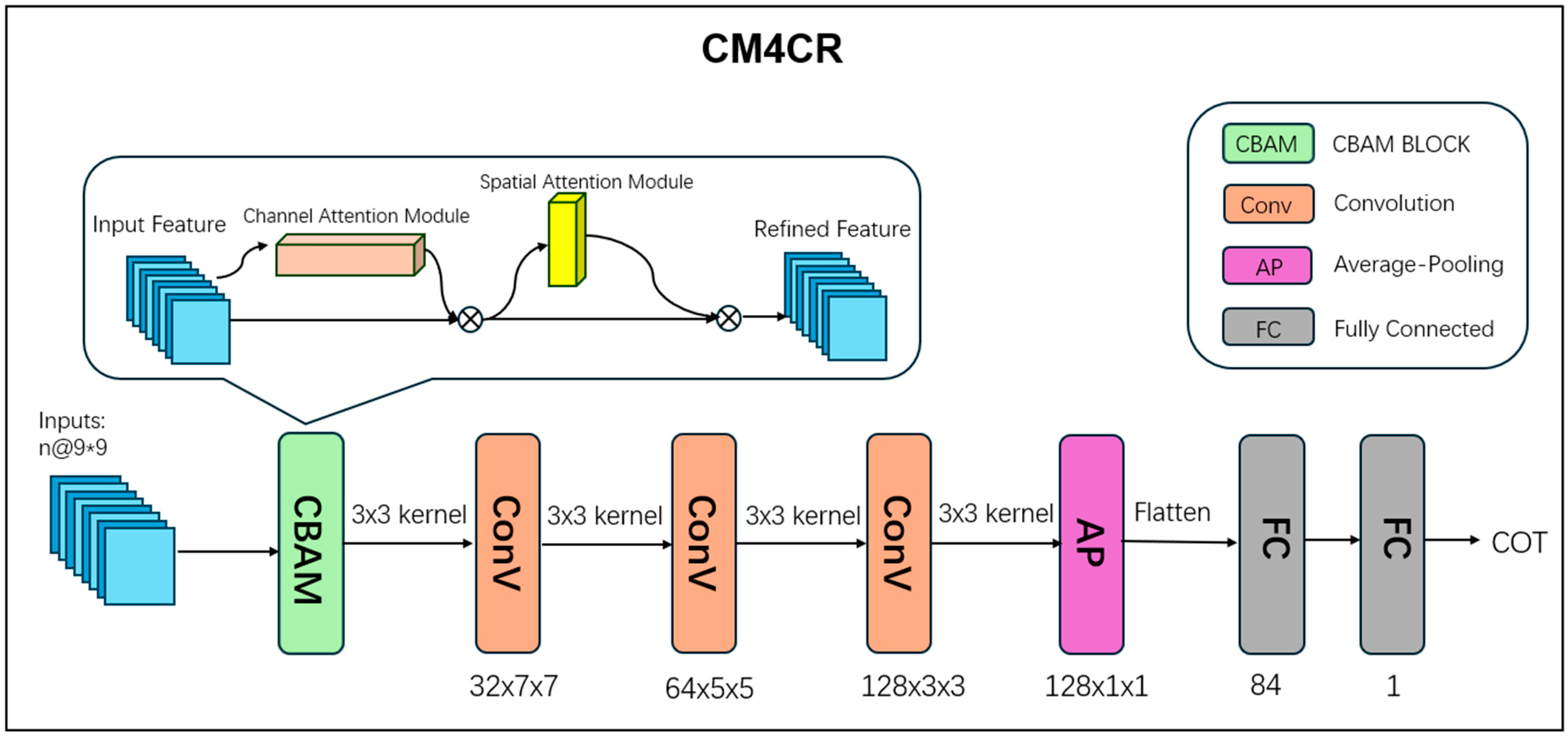
In this paper, we adopt a CNN architecture and develop a daytime cloud optical thickness retrieval model CM4CR based on FY-4A AGRI to retrieve COT values. We utilized the FY-4A satellite for COT retrieval. Although FY-4A does not currently provide cloud optical thickness (COT) products, it performs frequent Earth imaging in 14 spectral bands (L1 products). It offers various L2L3 products such as cloud type (CLT), quantitative precipitation estimation (QPE), cloud top temperature (CTT), and cloud phase (CLP). We selected 13 channels, including four basic bands, brightness temperature differences (BTD), cloud phase (CLP), as well as latitude, longitude, satellite zenith angle (SAZA), and solar zenith angle (SOZA), as input features. In addition to these 13 channels, we added three sets of additional bands to construct four datasets for training, validation, and testing. To fully extract these features, the Convolutional Block Attention Module (CBAM) is applied to CM4CR. CBAM is a simple yet effective attention module for feed-forward convolutional neural networks. It sequentially infers attention maps along two independent dimensions (channel and spatial) and then multiplies them with the input feature maps for adaptive feature refinement [21]. We used COT products provided by the CALIPSO satellite as ground truth for COT, ensuring accurate COT ground truth for network training. Then, a single-point matching method was adopted to reduce errors generated during the data-matching stage. To eliminate the spatiotemporal impact, we matched points by limiting the distance and time difference to 2 km and 3 min. Additionally, a multi-point averaging matching method was adopted to compensate for the horizontal distribution unevenness of clouds and the randomness of CALIPSO observation points. Finally, we created slices of size 9 × 9 centered around successfully matched single-point data for training CM4CR.

The characteristics of FY-4A AGRI products need to be considered to build a COT prediction method using COT data retrieved from FY-4A AGRI products. The time intervals between the adjacent FY-4A AGRI data are not fixed (ranging from 15 to 60 min). Additionally, cloud movements vary from calm to intense. This has inspired us to utilize a video prediction model for predicting COT, as in the video prediction domain, the spatial–temporal correlations across consecutive frames can be as heterogeneous as the COT prediction scenario is. The prediction of spatiotemporal sequences is a broad field, with significant research and work focused on video prediction [22,23,24,25,26]. The existing video prediction models have demonstrated their effectiveness on scientific datasets. Therefore, a deep learning method extended from a video prediction model is adopted to predict COT values based on the retrieval results obtained from CM4CR. The COT prediction model (CPM) consists of an encoder, a predictor, and a decoder. The COT values obtained from CM4CR serve as the input. Firstly, they are encoded by the Encoder to extract initial feature representations. Then, the predictor establishes spatiotemporal correlations among input space features and generates features for the predicted frames. Finally, the decoder decodes the features of the predicted frames into COT predictions in the same shape as the input. We augmented the traditional video prediction model by incorporating a time embedding module. Additionally, to enhance the detailed representation of predicted COT, we employed Charbonnier Loss and Edge Loss as the loss functions during the training phase. To enhance the model’s ability to learn from irregular time intervals, we augmented the architecture of the traditional video prediction model by adding a time embedding module. Additionally, to enhance the detailed representation of predicted COT, we utilized Charbonnier Loss and Edge Loss [27] as the loss functions during the training phase. We also investigated the impact of different lengths of COT input sequences and the time intervals between adjacent frames of COT on prediction performance.

The main contributions of this paper are summarized as follows:

• A daytime COT retrieval model based on CNN (CM4CR) has been designed, which enhances the neural network’s feature extraction capability by employing the CBAM module. Additionally, two matching methods, single-point matching, and multi-point average matching, have significantly reduced errors during data matching. Experimental results demonstrate that CM4CR achieves satisfactory retrieval performance.
• A COT prediction model CPM based on a video prediction model was developed. We incorporate a time embedding module to enhance its ability to learn from different time intervals and utilize Charbonnier Loss and Edge Loss during the training phase to improve the prediction of detailed information. We also explore how varying lengths of COT input sequences and the time intervals between adjacent COT frames affect prediction performance.

The rest of the paper is arranged as follows: Section 2 introduces recent work on COT retrieval and prediction in the meteorological domain. Section 3 presents the data sources and data-matching methods. Section 4 provides a detailed description of the architecture of CM4CR and the CPM. Section 5 presents experimental results and discussions. Finally, Section 6 summarizes the work of the entire paper.

2. Related Works

2.1. Retrieval of COT

The retrieval of cloud optical thickness has garnered widespread attention, with early efforts often relying on lookup tables (LUTs) based on traditional radiative transfer models for obtaining cloud optical thickness. Barnard et al. (2004) [28] proposed an empirical equation for estimating shortwave cloud optical thickness by measuring and analyzing shortwave broadband irradiance. When applied to a time series of broadband observations, this method can predict the distribution of cloud optical thickness. Kikuchi et al. (2006) [29] introduced a method to determine the optical thickness and effective particle radius of stratiform clouds containing liquid water droplets without drizzle by using measurements of solar radiation transmission. This method compares the measured cloud transmittance at wavelengths sensitive to water absorption and non-absorption with pre-calculated transmittance lookup tables for plane-parallel, vertically homogeneous clouds.

With the development of machine learning and the satellite industry, retrieval algorithms for cloud microphysical properties from satellite observations have rapidly evolved. The satellite-based cloud microphysical property retrieval field is mainly divided into LUT algorithms and deep learning methods. Letu et al. (2020) [10] used the LUT algorithm to retrieve cloud parameters based on Himawari-8 AHI products. They first determine the cloud phase using the brightness temperature (BT) band and the differences between the two BT bands. If the cloud is identified as a water cloud, the Mie–Lorenz scattering model is used to obtain the cloud optical thickness (COT) and Cloud Effective Radius (CER). If the cloud is an ice cloud, the Voronoi Ice Crystal Scattering (ICS) model is used. Liu et al. (2023) [11] employed the classical bi-spectral retrieval method for COT inversion based on FY4A AGRI products. They first use a machine learning algorithm (random forest) to detect the cloud mask (CMa) and cloud phase (CPH) as prerequisites for COT and CER retrieval. Then, using the optimal estimation method, they retrieve COT and CER based on the reflectance observed at the 0.87 μm and 2.25 μm channels, combined with the corresponding LUT.

Cloud microphysical property retrieval based on deep learning mainly develops neural network architectures, utilizing multi-channel products provided by passive satellites as inputs for network training. Kox et al. (2014) [12] proposed a method for cloud detection and retrieval of optical thickness and top height based on measurements from the Spinning Enhanced Visible and Infrared Imager (SEVIRI) instrument aboard the second-generation Meteosat (MSG) geostationary meteorological satellite. This method utilized a back-propagation neural network to train convolutional cloud optical thickness. Minnis et al. (2016) [13] developed the Infrared Cloud Optical Depth using the Artificial Neural Networks (ICODIN) method, which uses combinations of four thermal infrared and shortwave infrared channels to estimate the optical depth of opaque ice clouds during nighttime. In recent years, numerous attempts have indicated that deep learning algorithms, specifically convolutional neural networks (CNNs) or deep neural networks (DNNs), hold significant spatiotemporal potential in cloud remote sensing.

Deep-learning-based COT retrieval methods typically involve data matching. Effectively matching data between satellites to obtain more accurate and reliable true COT values is crucial for COT retrieval. However, existing studies often focus on the impact of different channels from various satellites on retrieval results while rarely exploring the errors introduced by the data-matching process. Wang X et al. (2022) [14] developed an image-based DNN algorithm that uses Himawari-8 AHI measured brightness temperatures from four thermal infrared bands as input to simultaneously retrieve CTH and COT in near-real time with satellite scanning. They used the nearest-neighbor interpolation method to match CALIPSO products with Himawari-8 AHI products. Wang Q et al. (2022) [15] developed a deep learning algorithm based on MODIS products to consistently retrieve daytime and nighttime cloud properties from passive satellite observations without auxiliary atmospheric parameters. They matched CALIPSO and MODIS products by constraining spatiotemporal conditions. Li et al. (2023) [16] developed a Transfer-Learning-Based approach to retrieve COT using Himawari-8 AHI products. They also matched Himawari-8 AHI products and MODIS products by constraining spatiotemporal conditions.

However, these studies often use a single-point matching method for data matching between different satellites. Due to the horizontal inhomogeneity within clouds and the inconsistency in data resolution between different satellites, using only single-point matching can result in significant errors. We employed a multi-point average matching method based on single-point matching to address this issue. The detailed matching process between FY4A AGRI and CALIPSO is described in Section 3.2.

2.2. Prediction in the Field of Meteorology

Traditional prediction methods typically involve researchers visually observing a large number of meteorological attributes’ features, recording them, and making predictions based on the recorded features. A typical example is the prediction of cloud cluster trajectories. Gong et al. (2000) predicted cloud cluster motion trajectories using a method based on motion vectors in MPEG-2 [30]. Lorenz et al. (2004) utilized the He-liosat2 method to obtain relevant indices of cloud images and combined it with motion vector methods to achieve cloud cluster motion prediction [31]. Yang et al. (2010) employed the concept of local thresholds to predict cloud clusters in ground-based cloud images [32]. Most traditional prediction methods are linear; however, atmospheric motion processes are not stationary but exhibit significant nonlinear variability. Therefore, traditional prediction methods often fail to produce accurate forecasts.

Meteorological attribute prediction has also made significant strides with the development of deep learning. Shi et al. (2015) proposed a Convolutional Long Short-Term Memory Neural Network (ConvLSTM) for predicting radar echo maps, achieving excellent prediction results [33], and ushering in a new era of spatiotemporal prediction research utilizing RNNs. ConvLSTM combines previous states’ spatial information through convolution, enabling the simultaneous extraction of spatial and temporal features. Subsequently, numerous researchers have developed many improved variant structures based on ConvLSTM. For example, Shi et al. (2017) [34] introduced the concept of optical flow trajectories. They proposed trajectory-gated recurrent Units (Traj GRU), which actively learn position change structures for recurrent connections, further enhancing prediction accuracy. Wang et al. (2017) proposed Spatiotemporal LSTM (ST-LSTM), which can simultaneously extract and retain spatial and temporal representations [35]. Requena-Mesa et al. (2021) combined Generative Adversarial Networks and LSTM networks to predict satellite cloud images [36]. Gao et al. (2022) proposed SimVP, which does not use complex modules such as RNNs, LSTMs, and Transformers, nor introduces complex training strategies such as adversarial training and curriculum learning, but only employs CNNs, skip connections, and MSE loss, providing a new direction for future research [22].

3. Data

3.1. Data Introduction

FY-4A is the first new-generation geostationary meteorological satellite in China. It was launched in 2016 and positioned at 104.7°E, providing continuous monitoring of the Eastern Hemisphere.FY-4A has four necessary instruments: Advanced Geostationary Radiation Imager (AGRI), Geostationary Interferometric Infrared Sounder (GIIRS), Lightning Mapping Imager (LMI), and Space Environment Package (SEP), among which the data we use are the products from AGRI.

AGRI is a multiple-channel radiation imager. It is technically featured by a precisely designed two-mirror structure, capable of accurate and flexible sensing in two dimensions and minute-level fast sector scanning. Frequent earth imaging over 14 bands ranging from 0.45 μm to 13.8 μm with three off-axis reflections of the primary optic system. The imaging time of AGRI in full disk mode is only 15 min. The enhanced spatiotemporal resolution of FY-4A/AGRI dramatically improves the detection and parameter retrieval capabilities. Specifically, the cloud retrievals of FY-4A have a spatial resolution of 4 km and a temporal resolution of 1 h [37]. We will use data from 2021 to train the CM4CR and from January to June 2022 for the test.

The observation area of FY4A/AGRI spans from 24.12°E to 185.28°E and from 80.57°S to 80.57°N. Each image comprises a non-uniform grid of 2748 × 2748 pixels, with a minimum spatial resolution of 4 km per pixel. In the regression experiments, we will adopt two data-matching methods (see Section 3.2) to match the observed data from FY4A AGRI and CALIPSO. We will only use the central 640 × 640 region for training and testing in the prediction experiments. The observed range of this region is approximately from 84.7°E to 124.7°E and from 40.57°S to 40.57°N.

CALIPSO was a joint NASA (USA) and CNES (France) environmental satellite, built in the Cannes Mandelieu Space Center, which was launched atop a Delta II rocket on 28 April 2006. Our research uses data from the CALIPSO Lidar level-2 5 km (V4.2) cloud vertical profile product as training ground truth for the regression model. It can be expressed as a collection of quadruples: Each quadruple’s elements represent longitude ($lo{n}_i$), latitude ($la{t}_i$), cloud optical thickness ($CO{T}_i$), and timestamp ($t_i$), respectively. Suppose the dataset of CALIPSO is denoted as $P_{\mathrm{CALIPSO}}$, then it can be represented as below:

$$P_{\mathrm{CALIPSO}}\in \left\{(lo{n}_1,la{t}_1,{\mathrm{COT}}_1,t_1),(lo{n}_2,la{t}_2,{\mathrm{COT}}_2,t_2),\dots ,(lo{n}_n,la{t}_n,{\mathrm{COT}}_n,t_n)\right\}$$

(1)

3.2. Data Processing

Our study collected data for the entire year of 2021, including full-disk pixels from FY-4A. FY-4A categorizes data into daytime, nighttime, and twilight based on Solar Zenith Angle (SOZA), where SOZA < 70° is defined as daytime. We specifically utilized data from the daytime period (2:00–8:00 UTC), with 11 frames of full-disk data available each -day. Disparity issues may introduce uncertainty, leading to significant pixel differences with higher Solar Zenith Angles (SAZA) [38]. As a result, the prediction accuracy of COT is compromised. Therefore, like most studies, we considered pixels with a high satellite zenith angle (SAZA > 70°) to be invalid.

The selection of retrieval bands also significantly impacts the retrieval of cloud optical thickness (COT). Internationally, satellites that release cloud optical thickness products include MODIS, VIIRS, GOES-R, and Himawari-8/9. For MODIS, the retrieval bands are channels 1, 2, 5, and 6, corresponding to central wavelengths of 0.66 µm, 0.86 µm, 1.24 µm, and 1.64 µm, respectively. VIIRS has similar inversion bands to MODIS, with central wavelengths of 0.67 µm, 0.87 µm, 1.24 µm, and 1.61 µm, respectively. Himawari-8/9 utilizes channels at 0.64 µm and 2.3 µm, two combination inversion bands capable of simultaneously retrieving cloud optical thickness and particle radius.

The retrieval of cloud optical thickness (COT) from various solar bands’ cloud reflection measurements has been extensively researched both theoretically and practically. FY-4A AGRI has 14 channels, as shown in

Table 1. Performance parameter of FY-4A AGRI.

Channel Number	Channel Type	Central Wavelength (µm)	Spectral Bandwidth (µm)	Spatial Resolution (km)
1	Visible light and near infrared	0.47	0.45~0.49	1
2		0.65	0.55~0.75	0.5~1
3		0.825	0.75~0.90	1
4	Shortwave infrared	1.375	1.36~1.39	2
5		1.61	1.58~1.64	2
6		2.25	2.10~2.35	2
7	Medium wave infrared	3.75	3.5~4.0 (high)	4
8		3.75	3.5~4.0 (low)	4
9	Water vapor	6.25	5.8~6.7	4
10		7.1	6.9~7.3	4
11	Long wave infrared	8.5	8.0~9.0	4
12		10.7	10.3~11.3	4
13		12.0	11.5~12.5	4
14		13.5	13.2~13.8	4

. Referring to the satellites mentioned above, the selected input channels for FY-4A AGRI are channels 2, 3, 11, and 12, with central wavelengths of 0.65 µm, 0.825 µm, 8.5 µm, and 10.7 µm, respectively. Let us then denote the set of the input bands. Furthermore, the cloud optical thickness algorithm has been described in the Algorithm Theoretical Basis Document (ATBD) of GEO (2021), emphasizing the sensitivity of Brightness Temperature Difference (BTD) T8.7–T10.8 to thermodynamic phases. Krebs et al. (2007) [39] designed various tests using the brightness temperature difference of multiple infrared bands from SEVIRI. The results indicate that the T10.8–T12 test can capture 90% of optically thick clouds, while the T8.7–T12 test effectively detects convective clouds with optical thicknesses between 0.5 and 10. This study will use the brightness temperature difference BTD of channels 11 (8.5 µm) and 12 (10.7 µm) as inputs, as shown in

Table 2. Summary of AGRI bands used in the model.

	Variable	Data Source	Spatial Resolution	Temporal Resolution
Daytime Input	0.65, 0.825, 8.5, 10.7 µm	FY-4A/AGRI	4 km	15 min
	T8.5 µm–T10.7 µm	FY-4A/AGRI	4 km	15 min

.

In addition to the Level 1 (L1) data provided by FY-4A AGRI, we also utilized their Level 2 (L2) and Level 3 (L3) products. This study selected Cloud Type (CLT) and Quantitative Precipitation Estimation (QPE) products to filter multi-layer cloud and precipitation pixels, focusing solely on single-layer clouds. Additionally, FY-4A Cloud Phase (CLP) products and some geophysical data, such as observed latitude and longitude, Satellite Azimuth Angle (SAZA), and Solar Zenith Angle (SOZA), were trained along with FY-4A bands as inputs for the model.

It is worth noting that among all input features, apart from CLP, which is a categorical feature, the rest are continuous features. Therefore, we need to handle CLP separately. Specifically, CLP represents the Cloud Phase product, and its values belong to the set {1: Water, 2: Super Cooled Type, 3: Mixed Type, 4: Ice Type}. We adopted a unique encoding format to adapt to our deep learning model. For each value, we represented it using a four-dimensional vector, mapping 1, 2, 3, and 4 to (1,0,0,0), (0,1,0,0), (0,0,1,0), and (0,0,0,1), respectively.

Combining the above information, the information for each period can form inputs for 13 channels, including Raw bands $\mathcal{W}$ during daytime, Brightness Temperature Difference (BTD), Cloud Phase (CLP), Longitude (lon), Latitude (lat), Satellite Zenith Angle (SAZA) and Solar Zenith Angle (SOZA). Each channel has 2748 × 2748 full-disc data and is normalized separately. Let $ℐ\in {ℝ}^{N\times H\times W}$ ($H=W=2748,N=13$) represent the input features, giving us the following:

$$ℐ=[\mathcal{W},\mathit{BTD},\mathit{CLP},\mathit{lon},\mathit{lat},\mathit{SAZA},\mathit{SOZA}]$$

(2)

Given a feature value $x_i$ in the original dataset, normalize it to the range [0, 1], the formula is given as follows:

$$x_i^{\mathrm{norm}}=\frac{x_i-\min \left(X\right)}{\max \left(X\right)-\min \left(X\right)}$$

(3)

where $x_i^{\mathrm{norm}}$ is the normalized feature value, $x_i$ is the feature value in the original dataset, and $\min \left(X\right)$ and $\max \left(X\right)$ are this feature’s minimum and maximum values in the original dataset, respectively.

Like the CALIPSO dataset, each observation point in the FY4A AGRI dataset also has an observation time, which we will utilize during the COT prediction phase for embedding time features.

In the retrieval experiments, we selected CALIPSO observational data as the ground truth for COT inversion. However, due to the deviation between the footprints of CALIPSO and FY-4A (Li et al., 2021) [40], to effectively address this issue, we opted for two methods for comparison: single-point matching and multi-point averaging matching.

3.2.1. Single-Point Data Matching

We constrained the distance and time difference between AGRI and CALIPSO pixels to within 2 km and 3 min, respectively, to eliminate the spatiotemporal effects. Then, within the constrained distance, we matched the selected points with the nearest CALIPSO scanning point (Liu et al., 2023 [11]; Xu et al., 2023 [41]). Subsequently, a 9 × 9 grid slice centered at the corresponding AGRI point was created for CNN training (Wu et al. [42], 2014; Zhang et al., 2014 [43]). Specifically, let the AGRI data point set be denoted as $P_{\mathrm{AGRI}}$ and the CALIPSO data point set as $P_{\mathrm{CALIPSO}}$, where each data point is composed of a quadruple $(lon,lat,\mathrm{COT},t)$. The matching process is defined as follows:

(a)

Based on the observation time of each element $p_{{\mathrm{CALIPSO}}_i}$ in the CALIPSO dataset, we locate the corresponding FY4A AGRI file for the respective period. Then, using the nominal formulas for converting between row and column numbers $p_{{\mathrm{AGRI}}_i}$ and geographical coordinates, we calculate the row and column numbers corresponding to the latitude and longitude of CALIPSO (rounded to the nearest integer).

(b)

We read the latitude and longitude information of the corresponding position from FY4A based on the row and column numbers. Then, using the Pyproj library, we calculate the distance d between the two points based on their latitude and longitude information. Afterward, we compute the time difference t between the observations of the two points.

(c)

If $d\le 2 \mathrm{km}$ and $t\le 3 \min$, then we consider the two points as matched.

(d)

For each matched AGRI data point, we create a grid slice centered at its spatial position, which is used for training the regression model.

$${\mathcal{S}}_{\mathrm{AGRI}}\left(p_{{\mathrm{AGRI}}_i}\right)=\{p_{\mathrm{AGRI}}\mid x_{\mathrm{AGRI}}\in [x_{{\mathrm{AGRI}}_i}-4,x_{{\mathrm{AGRI}}_i}+4],j\in [y_{{\mathrm{AGRI}}_i}-4,y_{{\mathrm{AGRI}}_i}+4]\}$$

(4)

where $p_{{\mathrm{AGRI}}_i}$ denotes a matched AGRI data point, $(x_{{\mathrm{AGRI}}_i},y_{{\mathrm{AGRI}}_i})$ represents the two-dimensional plane coordinates of this matched point, and ${\mathcal{S}}_{\mathrm{AGRI}}\left(p_{{\mathrm{AGRI}}_i}\right)$ denotes the $9\times 9$ grid slice created centered at this AGRI matched point.

3.2.2. Multiple-Point Averaging Matching

Due to the horizontal heterogeneity in clouds and the inconsistent data resolutions between CALIPSO and AGRI, errors may occur when mapping COT to AGRI, which can be potentially avoided with increased precision of grid data (Kox et al., 2014 [12]). Therefore, based on single-point matching, we apply a sliding window with a step size of 7 in CALIPSO for multiple-point averaging to compensate for the horizontal distribution heterogeneity of clouds and the randomness of CALIPSO observation points. Let ${\overline{p}}_{{\mathrm{CALPSO}}_i}$ denote the CALIPSO data point after multiple-point averaging for the matched point $p_{{\mathrm{CALPSO}}_i}$, then it can be calculated as follows:

$${\overline{p}}_{{\mathrm{CALIPSO}}_i}=\frac{1}{7}{\displaystyle \sum _{j=i-3}^{i+3}{p}_{{\mathrm{CALIPSO}}_j}}$$

(5)

In summary, the data-matching process involves Single-Point matching and Multiple-Point Averaging Matching. First, a CALIPSO point and its corresponding matching point on FY4A are identified, and their spatial and temporal information is checked for compliance with the requirements. If they meet the criteria, a 9 × 9 slice containing multi-channel information is created with the FY4A matching point as the center. Then, with the CALIPSO point as the center, a window consisting of seven consecutive CALIPSO points is taken, and the average COT value of these points within this window is calculated. This average value is used as the true COT value. Finally, the slice and the true COT value are stored together as a dataset.

4. Methodology

This paper’s research is divided into two phases: cloud optical thickness (COT) retrieval based on FY-4A AGRI data and COT prediction using the retrieval COT data as input. To accomplish this, we propose a COT retrieval model based on a Convolutional Neural Network (CNN) architecture (CM4CR) for COT retrieval and a COT Prediction Model (CPM) based on video prediction models for COT prediction. The research process is summarized in Figure 1.

4.1. Retrieval Model

This article’s process for retrieval COT can be divided into two stages: data preprocessing and model learning. The data preprocessing stage is detailed in Section 3.2, mainly involving the geolocation and radiometric calibration of the obtained FY-4A AGRI data, followed by grid processing. After filtering out invalid and duplicate values, the data are composed into multi-channel data. Subsequently, the data are normalized using the maximum–minimum normalization method. Finally, the AGRI data are matched with CALIPSO data to obtain several $n\times 9\times 9$ grids for model training, validation, and testing.

The structure of the CNN network, as shown in Figure 2, which has approximately 100,000 hyperparameters, is illustrated in the diagram. Initially, the multi-channel input data passes through the CBAM layer, where it undergoes a dual attention mechanism. The channel attention mechanism employs global average pooling to capture global channel-wise information, followed by learning channel attention weights through fully connected layers. Simultaneously, the spatial attention mechanism utilizes max pooling operations along rows and columns to identify salient channels for each spatial position, with spatial attention weights learned through additional fully connected layers. These attention maps are combined to optimize the features, resulting in enhanced representations that emphasize important channels and spatial regions, thus improving the network’s understanding and processing of the input data. Then, the refined inputs pass through three convolutional layers (each with a kernel size of 3 × 3) to extract features from the input data, including CLP, data from various bands, and longitude and latitude information. This process yields a 128-channel feature map. Subsequently, the feature map undergoes average pooling with a size of 3 × 3 to reduce the spatial dimensions of the feature map while retaining its essential information, resulting in a 128-channel feature map. Finally, the feature map is flattened and fed into two fully connected layers to map the feature vector to a size of 1 × 1, representing the retrieval COT value. $RCO{T}_i$ denotes the retrieved COT value by the model, $PCO{T}_i$ represents the corresponding COT value from CALIPSO’s ground truth point, and Loss denotes the error, giving us the following:

$$\mathrm{Loss}=\frac{1}{n}{\displaystyle \sum _{i=1}^n(}RCO{T}_i-PCO{T}_i{)}^2$$

(6)

4.2. Prediction Model

Through the CM4CR, we obtain 11 frames of COT values for each daytime, with each frame’s size being 640 × 640. We set horizontal and vertical strides to be 64, dividing the daily data into 100 groups of 64 × 64. We combine the 11 frames of data at the same position, where the first T frames serve as inputs and the following T′ frames are used as prediction frames to construct the dataset. Specifically, let $\mathcal{D}={\left(x_i,y_i\right)}_{i=1}^N$ denote the dataset constructed for prediction, where the goal of CPM $F(\cdot )$ is to map the input $x\in {ℝ}^{T\times C\times H\times W}$ to the target output $y\in {ℝ}^{T^{\prime }\times C\times H\times W}$. The learnable parameters of the model, denoted by $\Theta$, are optimized to minimize the following loss function:

$$\Theta ={\min }_{\Theta }\frac{1}{N}{\displaystyle \sum _{x,y\in D}L}\left(F_{\Theta }(x),y\right)$$

(7)

Here, $x\in {ℝ}^{T\times C\times H\times W}$ is the observed COT frame, and $y\in {ℝ}^{T^{\prime }\times C\times H\times W}$ is the future COT frame. C is the number of channels, T is the observed frame length, T′ is the future frame length, H is the height, and W is the width of the frames.

L denotes the loss function, where we use Charbonnier Loss and Edge Loss here. In contrast to L1 and L2 losses, which primarily focus on global loss, Edge Loss considers the influence of significant features, allowing for a more comprehensive consideration of texture differences and thereby improving the detailed representation of predicted COT. This is assuming that ${y^{\prime }}_i\in {ℝ}^{1\times 64\times 64}$ represents the COT prediction matrix obtained through the model ($y^{\prime }=F_{\Theta }\left(x\right)$) and $y_i\in {ℝ}^{1\times 64\times 64}$ represents the ground truth values of COT. Then, L can be calculated by the following formulas:

$$\begin{gathered} L=L_{\mathrm{char}}\left(y_i,{y^{\prime }}_i\right)+\lambda L_{\mathrm{edge}}\left(y_i,{y^{\prime }}_i\right), \\ {L}_{\mathrm{char}}=\sqrt{\Vert y_i-{y^{\prime }}_i{\Vert }^2+{\epsilon }^2}, \\ {L}_{\mathrm{edge}}=\sqrt{\Vert \Delta \left(y_i\right)-\Delta \left({y^{\prime }}_i\right){\Vert }^2+{\epsilon }^2} \end{gathered}$$

(8)

where $\epsilon$ is empirically set to ${10}^{-3}$ to avoid gradient vanishing and $\Delta$ denotes the Laplacian operator. The parameter $\lambda$ controls the relative importance of the two loss terms, which is set to 0.05 here.

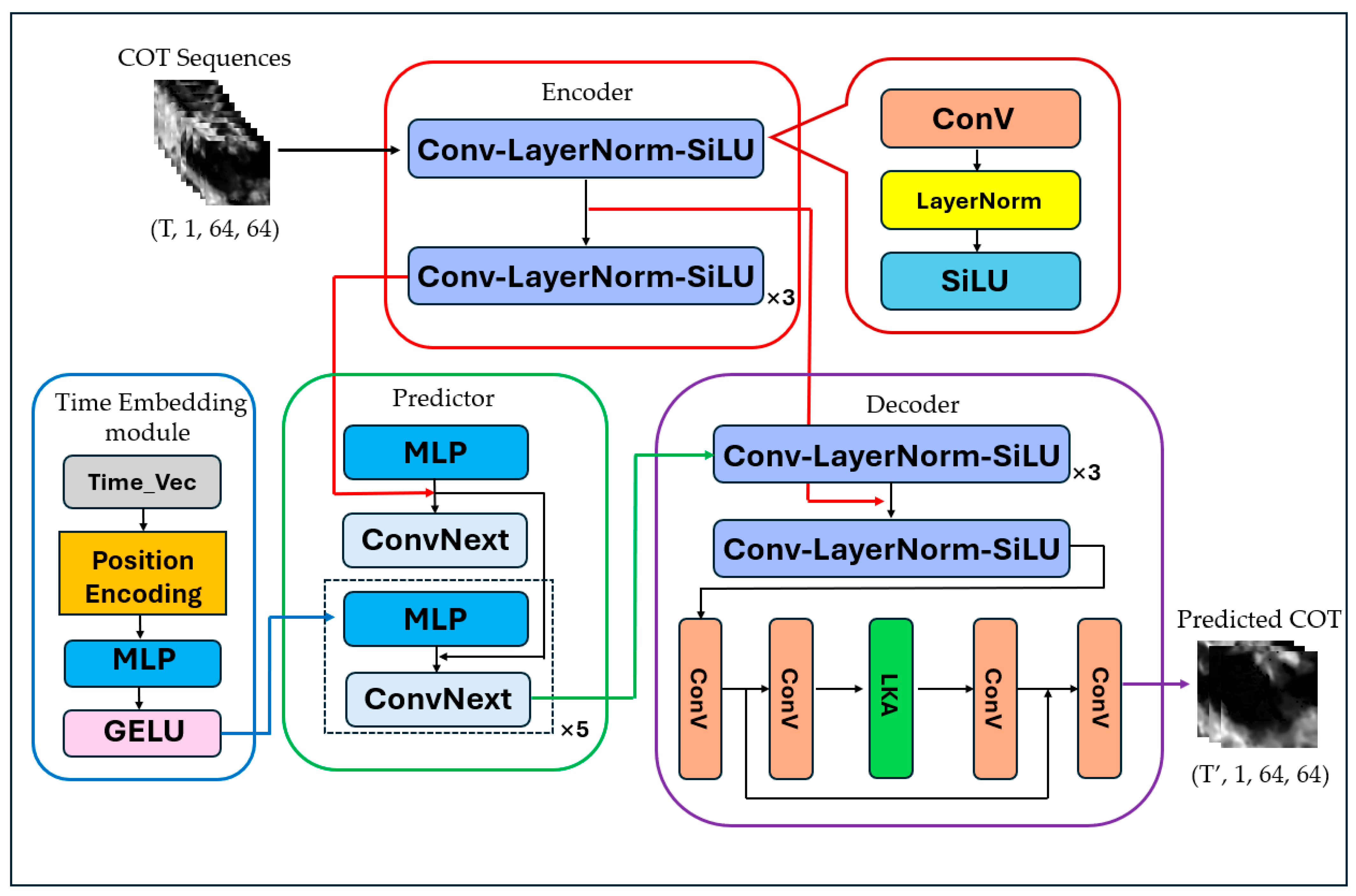
CPM follows the same architecture as existing mainstream prediction models, consisting of an encoder, a predictor, and a decoder. The encoder extracts features from the observed frame x and passes them to the predictor, which generates future features. Finally, the decoder decodes the future features to reconstruct the future frame y′. On this basis, we further incorporated a time embedding module. The architecture of the CPM is shown in Figure 3.

4.2.1. Encoder

The Encoder module serves the essential function of encoding input cloud optical thickness (COT) values to derive effective feature representations. This process is facilitated by the utilization of convolutional layers (ConvSC), enabling the progressive downsampling of feature maps alongside an augmentation in channel dimensions. Such architectural design aligns closely with the conventions observed in convolutional neural networks (CNNs) commonly deployed for image classification tasks, wherein spatial information is incrementally aggregated to extract abstract and high-level features.

In the context of daytime data collection via the CM4CR, a sequence of 11 frames of COT values is obtained daily. The Encoder operates on the normalized frames from the initial T frames as input, which results in an input tensor shape of $T\times 1\times 64\times 64$. The Encoder’s architectural configuration, as illustrated in Figure 3, consists of 4 Convolution-Layer Normalization-SiLU (Conv-LayerNorm-SiLU) layers. Remarkably, the output from the first layer is integrated into the decoder through skip connections, while the fourth layer yields spatial features characterized by 128 channels. These spatial representations are subsequently transmitted to the Predictor module for further processing.

4.2.2. Predictor

The primary function of the Predictor module revolves around forecasting forthcoming cloud optical thickness (COT) features by leveraging the encoded representations extracted by the Encoder. It adopts a spatial–temporal prediction architecture characterized by ConvNeXt blocks, notable for their utilization of causal convolutions along the temporal axis. These ConvNeXt blocks are strategically integrated to augment the model’s spatial–temporal modeling capabilities. Within each block, essential components including depth wise separable convolutions, Layer Normalization, and Multi-Layer Perceptron (MLP) are harnessed, collectively facilitating the effective capture of the intricate nonlinear dynamical characteristics inherent in COT data. The module orchestrates gradual transformations and updates of feature maps to realize predictions of future COT values with precision and fidelity.

Additionally, the Predictor also integrates time information as additional input, enabling the model to better understand the irregular time intervals of the COT sequence. A time embedding module is used to encode the time information of the input data and output a feature vector. This feature vector, along with the output features of the encoder, is input into the Predictor.

Let the original time information of a set of COT sequences be $T\in [T_1,T_2,\dots ,T_t]$, where $T_i$ represents UTC when scanning begins for the ith frame of COT information. The corresponding embedded time information feature vector is $t\in [t_1,t_2,t_3,\dots t_t]$, where $t_i=t_i-t_1(i>1)$ denotes the time difference between the ith frame of COT information and the first frame (in seconds). The time embedding module encompasses two key components: a positional encoding module and a Feed-Forward Network (FFN) integrated with the GELU [44] activation function. The initial encoding of time features adopts sinusoidal positional encoding [45], which furnishes a distinctive representation for each position and encapsulates relative positional relationships through the periodicity of sine and cosine functions. Notably, every element within the input vector undergoes positional encoding, resulting in the generation of a vector with a size of 64. Subsequently, this encoded vector is subjected to two layers of fully connected networks, culminating in the derivation of a time feature vector also with a size of 64.

4.2.3. Decoder

The primary function of the Decoder module entails the gradual amplification and decoding of low-resolution prediction feature maps generated by the Predictor, with the objective of reconstructing COT values commensurate with the input dimensions of 64 × 64. This process involves the utilization of transposed convolutional layers combined with a linear attention named large kernel attention (LKA) [46], strategically implemented to incrementally enhance the resolution of the feature maps. Furthermore, the Decoder integrates these refined features with shallow representations extracted by the Encoder, thereby facilitating the extraction of nuanced prediction details. An imperative aspect of the Decoder’s functionality lies in its adeptness at amalgamating feature information originating from diverse scales, an endeavor critical for attaining high-fidelity prediction outcomes during the decoding phase.

By harnessing the shallow features furnished by the Encoder, the Decoder adeptly synthesizes high-frequency information, thereby preserving global structural coherence whilst concurrently reinstating intricate prediction particulars. Notably, the strategic incorporation of skip connections, a well-established paradigm notably efficacious in domains such as image segmentation and super-resolution, is instrumental in bolstering the perceptual fidelity of the resultant predictions. Finally, the Decoder subjects its output to a 1 × 1 convolutional layer, thereby effectuating the derivation of COT prediction outcomes characterized by dimensions congruent with those of the input.

Table 3. The detailed breakdown of CPM. T represents the length of the input sequence, and T′ represents the length of the output sequence.

Layer	Sub Layer	Input	Output
Encoder	Conv-LayerNorm-SiLU Conv-LayerNorm-SiLU (×3)	COT Sequences: (T, 1, 64, 64) Enc_1	Enc_1: (T, 128, 64, 64) Enc_2: (T, 128, 16, 16)
Time Embedding Module	Position Encoding Linear GELU Linear	Time_Vec: (T) Time_Vec (T, 64) Time_Vec (256) Time_Vec (256)	Time_Vec: (T, 64) Time_Vec: (256) Time_Vec: (256) Time_Vec: (64)
Predictor	Reshape	hyper-parameter: (T, 128, 16, 16) Enc_2	Prediction: (2560, 16, 16)
	ConvNeXt	Prediction	Prediction: (1280, 16, 16)
	Linear	Time_Vec	Time_emb: (128)
	Add	Prediction, Time_emb	Prediction: (1280, 16, 16)
	ConvNeXt	Prediction	Prediction: (1280, 16, 16)
	Linear	Time_Vec	Time_emb: (128)
	Add	Prediction, Time_emb	Prediction: (1280, 16, 16)
	ConvNeXt	Prediction	Prediction: (1280, 16, 16)
	Linear	Time_Vec	Time_emb: (128)
	Add	Prediction, Time_emb	Prediction: (1280, 16, 16)
	Linear	Time_Vec	Time_emb: (128)
	ConvNeXt	Prediction	Prediction: (1280, 16, 16)
	Linear	Time_Vec	Time_emb: (128)
	Add	Prediction, Time_emb	Prediction: (1280, 16, 16)
	ConvNeXt	Prediction	Prediction: (1280, 16, 16)
	Linear	Time_Vec	Time_emb: (128)
	Add	Prediction, Time_emb	Prediction: (1280, 16, 16)
	Reshape	Prediction	Prediction: (T, 128, 16, 16)
Decoder	Transposed Conv-LayerNorm-SiLU	Prediction	Dec: (T, 128, 16, 16)
	Transposed Conv-LayerNorm-SiLU	Dec	Dec: (T, 128, 32, 32)
	Transposed Conv-LayerNorm-SiLU	Dec	Dec: (T, 128, 64, 64)
	Add	Dec, Enc_1	Dec: (T, 256, 64, 64)
	Transposed Conv-LayerNorm-SiLU	Dec	Dec: (T, 128, 64, 64)
	Reshape	Dec	Dec: (1280, 64, 64)
	2D Convolution (1 × 1)	Dec	Dec: (64, 64, 64)
	Large Kernel Attention	Dec	Dec: (64, 64, 64)
	2D Convolution (1 × 1)	Dec	Output: (T′, 64, 64)

shows the detailed structure of CPM.

5. Experiments

5.1. Setup

The COT retrieval experiments were conducted using a system equipped with an NVIDIA GeForce RTX 2060 GPU (6GB VRAM), an Intel^® Core (TM) i7-10875H CPU @ 2.30 GHz (16 cores), and 16GB of RAM. The system ran on Ubuntu 22.04 and utilized Python 3.10.13 as the interpreter, with NumPy 1.26.0 and PyTorch 2.1.0 libraries. Model training employed the Adam optimizer with a learning rate of 0.001, beta1 of 0.9, beta2 of 0.999, and weight decay set to 0. The Mean Squared Error (MSE) loss function was utilized, with a batch size of 64.

The COT prediction experiments were conducted using a system equipped with an NVIDIA RTX 4090 GPU, an Intel(R) Core (TM) i7-13700F CPU, and 64GB of RAM. The system ran on Windows 11 22H2 operating system and utilized Python 3.10.13 as the interpreter, with NumPy 1.26.0 and PyTorch 2.1.0 libraries. Model training employed the Adam optimizer with a learning rate of 0.001, β1 of 0.9, and β2 of 0.999. The Charbonnier Loss function and Edge Loss function were utilized, with a batch size set to 10.

5.2. Metrics

5.2.1. Root Mean Square Error (RMSE)

The Root Mean Square Error (RMSE) is calculated as the regression model evaluation metric using the following formula:

$$\mathrm{RMSE}=\sqrt{\frac{1}{n}{\displaystyle \sum _{i=1}^n(}CO{T}_i-\widehat{C}O{T}_i{)}^2}$$

(9)

where n represents the total number of COT data used for calculating RMSE, $CO{T}_i$ denotes the actual observed value of the ith COT, and $\widehat{C}O{T}_i$ represents the predicted value of the ith COT. A smaller RMSE value indicates better predictive capability of the model, as it indicates less difference between the predicted values of the model and the actual observed values.

5.2.2. Mean Absolute Error (MAE)

The formula for MAE (Mean Absolute Error) is as follows:

$$\mathrm{MAE}=\frac{1}{n}{\displaystyle \sum _{i=1}^n|}CO{T}_i-\widehat{C}O{T}_i|$$

(10)

where n represents the total number of COT data used for calculating MAE, $CO{T}_i$ denotes the actual observed value of the ith COT, and $\widehat{C}O{T}_i$ represents the predicted value of the ith COT. MAE measures the average absolute difference between predicted and actual values. A smaller MAE indicates better predictive performance of the model.

5.2.3. The Coefficient of Determination ($R^2$)

The coefficient of determination, commonly known as the R-squared ($R^2$), is used in statistics to measure the proportion of the variance in the dependent variable that is predictable from the independent variable(s), indicating the explanatory power of the regression model. For simple linear regression, the coefficient of determination is the square of the sample correlation coefficient, expressed by the following formula:

$$R^2=1-\frac{{\displaystyle \sum _{i=1}^n(}CO{T}_i-\widehat{C}O{T}_i{)}^2}{{\displaystyle \sum _{i=1}^n(}CO{T}_i-\overline{COT}{)}^2}$$

(11)

where n represents the total number of COT data used for calculating $R^2$, $CO{T}_i$ denotes the actual observed value of the ith COT, $\widehat{C}O{T}_i$ represents the predicted value of the ith COT, and $\overline{COT}$ represents the average value of the actual COT.

5.2.4. Structural Similarity Index (SSIM)

The Structural Similarity Index (SSIM) is a metric used to compare the similarity between two images, taking into account not only their brightness and contrast but also their structural information. The calculation of SSIM involves three aspects of comparison: luminance, contrast, and structure. Given two images, namely x and y (in this context, representing grayscale images composed of actual and predicted COT values normalized), with respective mean values of ${\mu }_x$ and ${\mu }_y$, variances of ${\sigma }_x^2$ and ${\sigma }_y^2$, and a covariance of ${\sigma }_{xy}$, the Structural Similarity Index (SSIM) is defined as:

$$\mathrm{SSIM}(x,y)=\frac{(2{\mu }_x{\mu }_y+C_1\left)\right(2{\sigma }_{xy}+C_2)}{({\mu }_x^2+{\mu }_y^2+C_1\left)\right({\sigma }_x^2+{\sigma }_y^2+C_2)}$$

(12)

$C_1$ and $C_2$ are constants used for stabilizing the calculation, typically set as $C_1={\left(K_{1}L\right)}^2$ and $C_2={\left(K_{2}L\right)}^2$, where L is the dynamic range of pixel values, and $K_1$ and $K_2$ are constants, usually set as $K_1=0.01$ and $K_2=0.03$. In practical applications, the value of SSIM typically ranges from 0 to 1, where 1 indicates perfect similarity between two images, and 0 indicates complete dissimilarity.

5.2.5. Structural Similarity Index (SSIM)

PSNR (Peak Signal-to-Noise Ratio) is a metric used to measure the quality of an image, commonly employed to assess the similarity between an original image and a compressed or distorted version. The calculation of PSNR is based on the Mean Squared Error (MSE) of the image, and its mathematical definition is as follows:

$$\mathrm{PSNR}=10\cdot {\log }_{10}\left(\frac{{\mathrm{MAX}}^2}{\mathrm{MSE}}\right)$$

(13)

where MAX represents the maximum possible value of the data type. In image processing, typically, the pixel values are in the range of [0, 255]; thus, MAX is usually set to 255. MSE denotes the Mean Squared Error, namely $MSE=RMS{E}^2$. PSNR is measured in decibels (dB). A higher PSNR value indicates better image quality because its corresponding MSE is lower. The typical range of PSNR values is between 20 dB and 50 dB.

5.3. COT Retrieval Experiment Results

In this study, considering only single-layer clouds and daytime data (SOZA < 70°) while disregarding low-quality data with SAZA > 70°, we established a scientifically reliable optical thickness retrieval dataset using both single-point matching and multi-point averaging matching methods. To enhance the model’s learning capability and robustness, we augmented the original daytime raw bands with additional bands, resulting in four datasets for model training, as shown in

Table 4. The constructed dataset and the central wavelengths of the additional bands.

Dataset	Original Input	Additional Bands (µm)
1	$ℐ=[\mathcal{W},\mathit{BTD},\mathit{CLP},\mathit{lon},\mathit{lat},\mathit{SAZA},\mathit{SOZA}]$	null
2		0.47, 1.61, 1.21
3		1.37, 1.61, 2.22
4		1.61, 1.22.

.

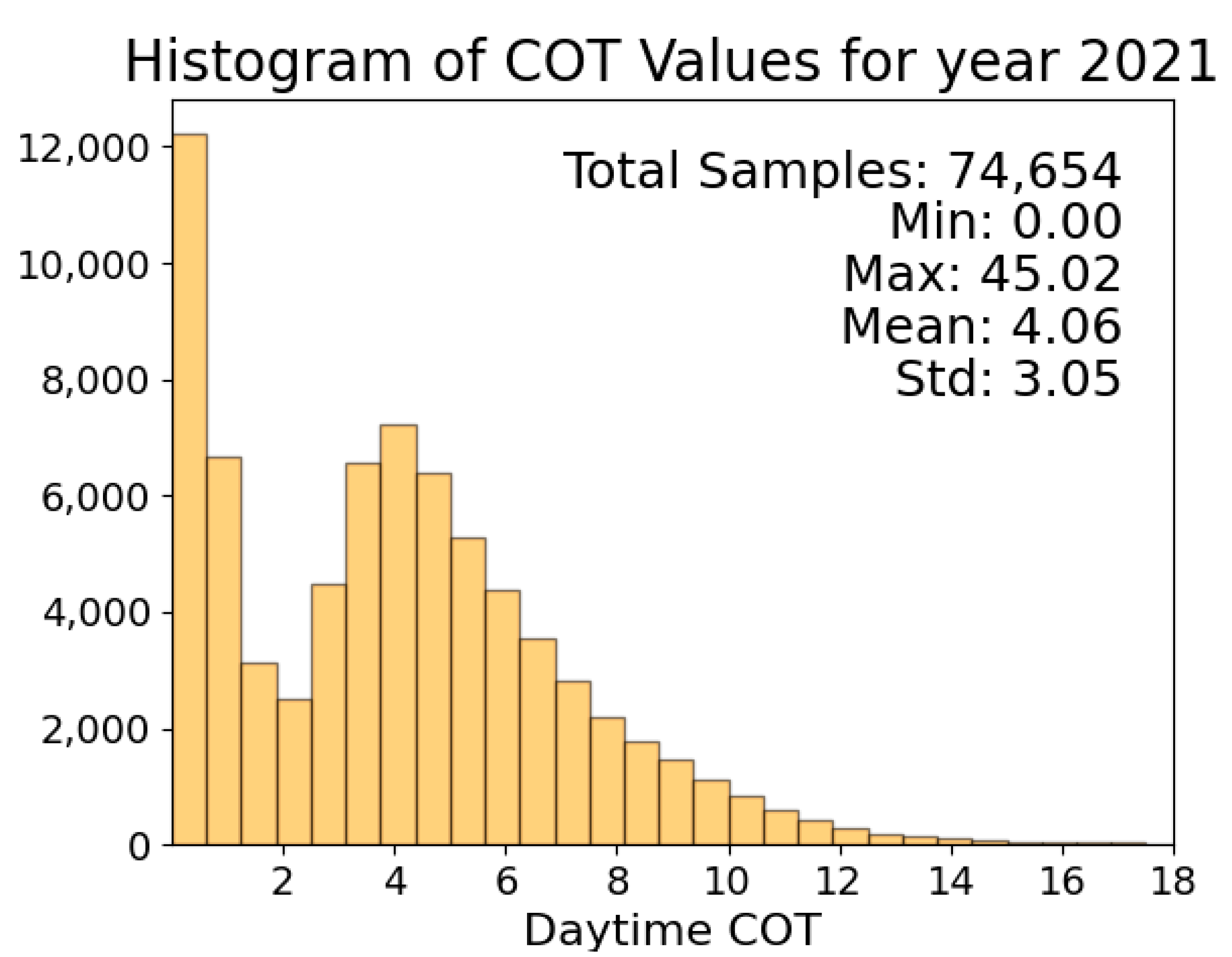
Considering the CALIPSO multi-point averaged matching values as the ground truth for COT, a histogram illustrating the distribution of COT values for the year 2021 is plotted, as depicted in Figure 4. It can be observed that in regions where SAZA < 70°, the distribution of daytime COT concentrates is between 0–1 and 3–5, with a maximum COT value of 45.02. The mean COT value is 4.06, with a standard deviation of 3.05.

We used data from the year 2021 for training and validation. Specifically, after data matching, we obtained 74,654 data samples, of which 59,723 were used for training and 14,931 were used for validation. The model was then evaluated using data from January to June 2022 as the test set. The scatter density plot in Figure 5a illustrates the model’s performance on the test set, accompanied by metrics such as RMSE, R², MAE, etc. As shown in Figure 5a, the R² on the test set is 0.75, with an RMSE of 1.26 and MAE of 0.86 Additionally, the histogram in Figure 5b depicts the distribution of predicted and actual values. It is evident that the predicted values are generally lower than the actual values, but the distributions roughly align. Moreover, the maximum predicted value is 13.05, whereas the maximum actual value is 20.78, indicating that the model lacks learning capability in the region of thick optical clouds (COT > 12).

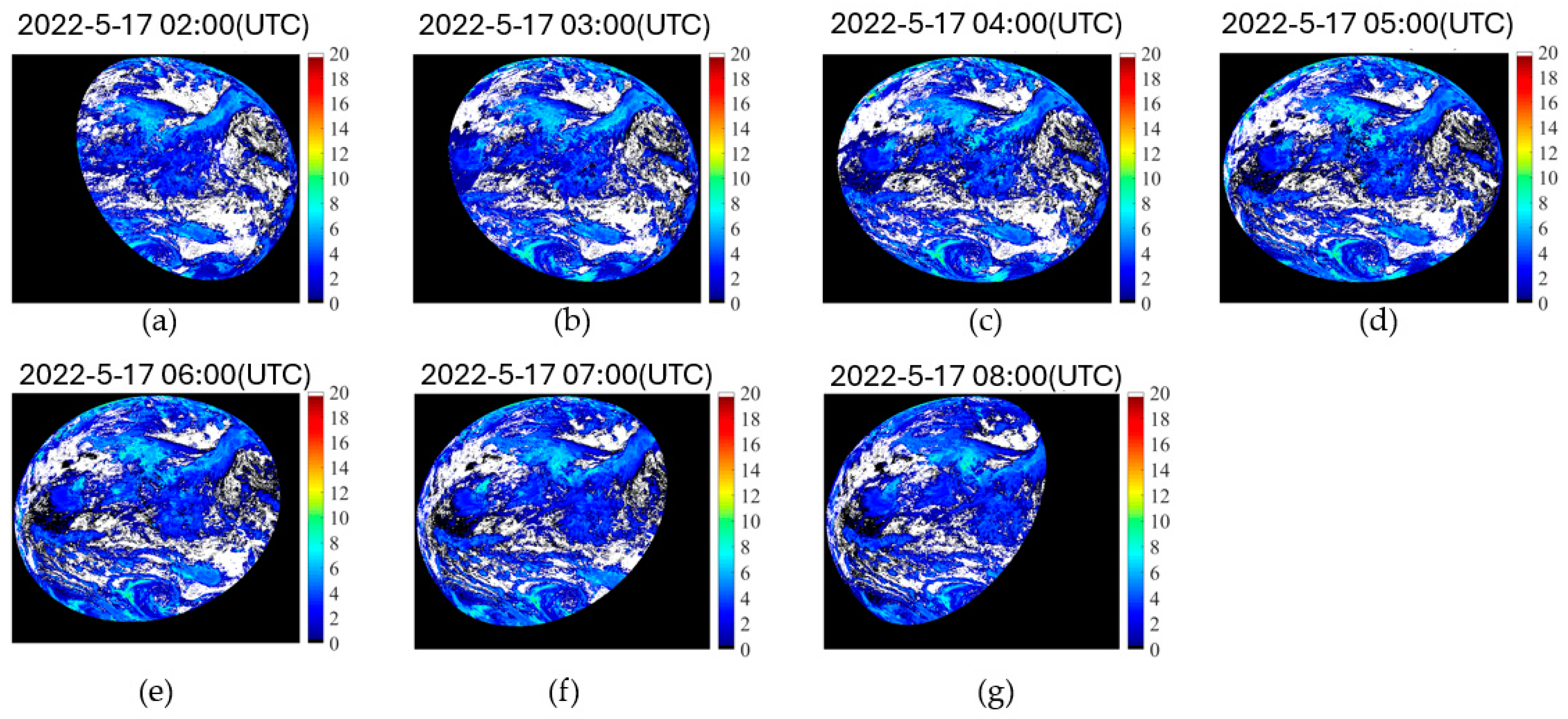
Letu et al. (2020) [10] used the LUT algorithm based on Himawari-8 AHI products to retrieve cloud parameters, achieving an R² of 0.59 for water clouds and an R² of 0.72 for ice clouds. Wang et al. (2022) [15] utilized a CNN model based on MODIS products to retrieve daytime COT and conducted a consistency assessment with MYD06 products, resulting in an R² of 0.62. Liu et al. (2023) [11] used the classic dual-channel retrieval method based on FY4A AGRI products for COT retrieval and compared it with MODIS products, obtaining an R² of 0.58. In contrast, our CM4CR algorithm, based on the multi-channel products provided by FY4A AGRI and employing a scientific data-matching method with CALIPSO products, achieved an R² of 0.75, demonstrating superior COT retrieval performance. Figure 6 displays the COT retrieval results based on the CM4CR model for 17 May 2022 from 2:00 to 8:00 UTC.

Through research on COT retrieval experiments, we found that the retrieved COT values are generally lower than the actual COT values. Some samples remain in the optically thick cloud region (COT > 12). However, the retrieval model’s prediction results rarely include this optically thick cloud region, with no predicted values. This phenomenon may be due to a lack of higher COT values in the input data used to train the CNN model. Therefore, to ensure overall training effectiveness during the training process, the CNN model tends to undergo multiple rounds of learning in the distribution range of the sample set (0~7). The optically thick cloud region is considered tail data, resulting in reduced learning.

Simultaneously, we conducted a set of ablation experiments to verify the enhancement in retrieval performance brought by adding brightness temperature differences and latitude and longitude information, as well as a comparison between using single-point matching and multi-point average matching for retrieval.

Table 5. Retrieval results for different input information and data-matching methods. The RMSE and R² in the table are calculated after denormalization.

Input	Matching Method	RMSE	R2
$ℐ=[\mathcal{W},\mathit{BTD},\mathit{CLP},\mathit{lon},\mathit{lat},\mathit{SAZA},\mathit{SOZA}]$	Single-Point Data Matching	1.99	0.57
$ℐ=[\mathcal{W},\mathit{CLP},\mathit{SAZA},\mathit{SOZA}]$	Multiple-Point Averaging	1.37	0.71
$ℐ=[\mathcal{W},\mathit{BTD},\mathit{CLP},\mathit{lon},\mathit{lat},\mathit{SAZA},\mathit{SOZA}]$	Multiple-Point Averaging	1.26	0.75

shows the impact of different bands and matching methods on the retrieval results. The RMSE of the retrieval results obtained using only band, SAZA, and SOZA information is 1.37, and the $R^2$ is 0.71. After adding brightness temperature differences and latitude and longitude information, the RMSE of the retrieval results is 1.26, and the $R^2$ is 0.75. This indicates that the model’s learning ability has been improved with the addition of brightness temperature differences and latitude and longitude information. Moreover, if only single-point matching is used for data matching, the resulting retrieval RMSE is 1.99 and the $R^2$ is 0.57, which is inferior to the results obtained using multi-point average matching. This also demonstrates that performing multi-point average matching based on single-point matching can effectively address issues such as horizontal inhomogeneity within clouds and errors caused by the resolution mismatch between CALIPSO and AGRI data.

5.4. COT Prediction Experiment Results

We introduced two baseline models for deep-learning-based video prediction to demonstrate the effectiveness of CPM: ConvLSTM and SimVP.

ConvLSTM: a type of recurrent neural network for spatio-temporal prediction that has convolutional structures in both the input-to-state and state-to-state transitions. The ConvLSTM determines the future state of a certain cell in the grid by the inputs and past states of its local neighbors. This is achieved by using a convolution operator in the state-to-state and input-to-state transitions.

SimVP: A simple yet effective CNN video prediction model. SimVP achieves state-of-the-art results without introducing any complex modules, strategies, or tricks. Additionally, its low computational cost makes it easy to scale to more scenarios. SimVP has become a powerful baseline in the field of video prediction.

The optimizer, learning rate, and batch size used during the training of the above models are the same as those used for the CPM configuration, and the MSE loss function was used in SimVP and ConvLSTM.

In the prediction phase, we used the retrieval COT results from daytime (2:00–8:00 UTC) in 2021 as the dataset, with 70% of this data for training, 10% for validation, and 20% for testing. We cropped the central 640 × 640 region from the retrieval results of the full disk. The input shape of the prediction model is [Batch Size, T, 1, 64, 64], representing the input of the first T frames. In this experiment, as shown in

Table 6. Input sequence and output sequence.

Sequence Length	Input Sequence	Output Sequence
$T=5,T^{\prime }=5$	$\left[t_1,t_2,t_3,t_4,t_5\right]$	$\left[t_6,t_7,t_8,t_9,t_{10}\right]$
$T=8,T^{\prime }=3$	$\left[t_1,t_2,t_3,t_4,t_5,t_6,t_7,t_8\right]$	$\left[t_9,t_{10},t_{11}\right]$
$T=8,T^{\prime }=2$	$\left[t_2,t_3,t_4,t_5,t_6,t_7,t_8,t_9\right]$	$\left[t_{10},t_{11}\right]$
$T=10,T^{\prime }=1$	$\left[t_1,t_2,t_3,t_4,t_5,t_6,t_7,t_8,t_9,t_{10}\right]$	$\left[t_{11}\right]$

, we set T = {5, 8, 8, 10}, and correspondingly set T′ = {5, 3, 2, 1} to explore the effects of time intervals and input sequence lengths on prediction results. Meanwhile, we compared CPM with the other two baseline models at T = 10 to demonstrate its effectiveness.

We randomly shuffled the 2021 dataset, yielding 100 data samples daily. During the model training phase, we used data from 255 days, totaling 255,000 input data samples. The validation set comprised data from 36 days, amounting to 36,000 validation data samples. The test set included data from 74 days, resulting in 74,000 test data samples. During training, we employed the OneCycleLR scheduler to dynamically adjust the learning rate throughout the training process, aiming to enhance training effectiveness. The working principle of the OneCycleLR scheduler is to gradually increase the learning rate from a small value to a maximum value in the early stages of training and then gradually decrease it in the later stages. This learning rate variation pattern helps accelerate model convergence and prevents overfitting in the later stages of training. More specifically, at step during training, the learning rate is calculated using the following formula:

$$lr=l{r}_{max}\times \left(\frac{1+\cos \left(\frac{\pi \times \mathrm{step}}{\mathrm{total}\_\mathrm{steps}}\right)}{2}\right)$$

(14)

where $l{r}_{max}$ is the specified maximum learning rate (set to 0.01 in this experiment), step is the current training step, and $total\_steps$ is the total number of training steps.

This section compares the prediction results of CPM with those of the other two baseline models when the input sequence length is 10 and the prediction sequence length is 1.

To quantify the effectiveness of each model, we utilized the metrics mentioned in Section 5.1, including RMSE, MAE, SSIM, and PSNR, for comprehensive evaluation. The performance comparison between CPM and baseline models is presented in

Table 7. The comparison of 4 metrics between CPM and baseline models. The RMSE and MAE shown in the table are calculated after denormalization. The arrow after the metric indicates whether CPM has increased or decreased compared to other models.

Model	RMSE↓	MAE↓	SSIM↑	PSNR↑	RMSE′↓	R2↑
ConvLSTM	1.114	0.889	0.2994	19.0386	1.3480	0.48
SimVP	0.882	0.626	0.4396	29.2083	1.2758	0.53
CPM (ours)	0.878	0.560	0.5197	29.9403	1.2670	0.54

. The results indicate that CPM outperforms other baseline models significantly. Figure 7a–c illustrate scatter density plots for 10,000 pairs of points from the test set across the three models. To provide a more reliable assessment and validation of the results, we matched all prediction results with CALIPSO products according to the matching method described in Section 3.2. This process yielded 992 matched points. We then calculated the RMSE and R² between these matched points and the CALIPSO COT products. Detailed data can be found in the last two columns (RMSE′ and R²) of Table 5. Compared to the other two baseline models, CPM demonstrated better prediction performance.

Table 8. The RMSE of predicted COT values at different time points for varying lengths of input sequences. The RMSE in the table is calculated after denormalization.

Sequence Length	RMSE at Different Time Points: Δt(Frame Number)
	60(6)	45(7)	15(8)	15(9)	45(10)	60(11)	Total
T = 5, T′ = 5	1.232	1.348	1.345	1.335	1.315	null	1.315
T = 8, T′ = 3	Input	Input	Input	0.611	0.914	1.078	0.868
T = 8, T′ = 2	Input	Input	Input	Input	0.827	1.067	0.947
T = 10, T′ = 1	Input	Input	Input	Input	Input	0.878	0.878

presents the RMSE of predicted COT values at different time points compared to the ground truth values for varying lengths of input sequences in CPM. The leftmost column of the table indicates the input sequence length and the prediction sequence length, while the second row represents the time difference between each time point and the previous time point (in minutes). The number in brackets is the frame number. Each column in the table (excluding the last column) represents the RMSE for a specific time point, and the last column shows the RMSE for all prediction time points.

The experimental results show that when predicting three frames and two frames of COT with an input of 8 frames, there is a trend of increasing RMSE, known as the “error accumulation” phenomenon in the field of time series prediction. By comparing T = 8, T′ = 3 and T = 8, T′ = 2, we found that when predicting the 10th frame of COT, the RMSE is 0.827 for T = 8, T′ = 2, and 0.914 for T = 8, T′ = 3. The prediction results of T = 8, T′ = 2 are better, which indicates that the first directly predicted frame usually performs best since no “error accumulation” phenomenon exists. Additionally, when T = 8 and T′ = 3, the time difference between the first predicted frame of COT and the last input frame of COT is only 15 min, resulting in an RMSE of 0.611, achieving the best prediction performance. Therefore, shorter time intervals also improve prediction accuracy. Moreover, when comparing T = 5, T′ = 5, and T = 10, T′ = 1, where the time difference between the first predicted frame of COT and the last input frame of COT is 60 min for both, the RMSE is 1.232 for the former and 0.878 for the latter, indicating that a more extended input sequence significantly enhances the prediction performance.

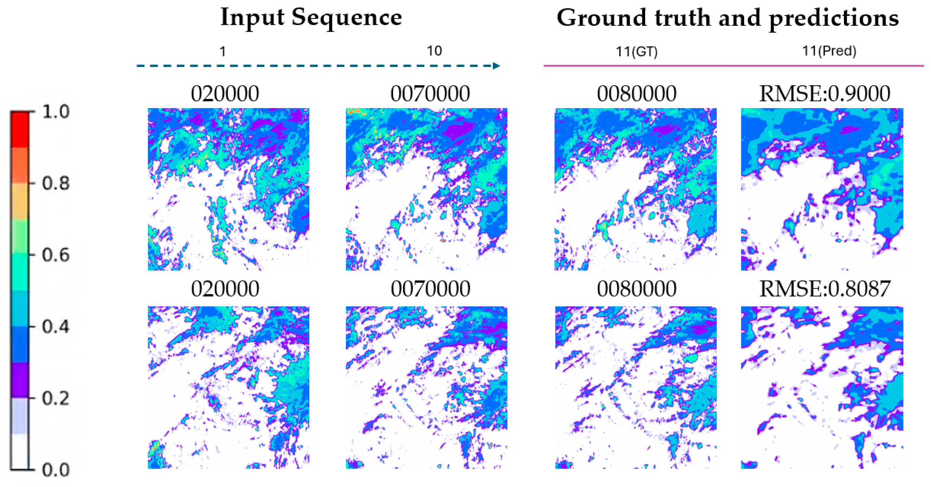
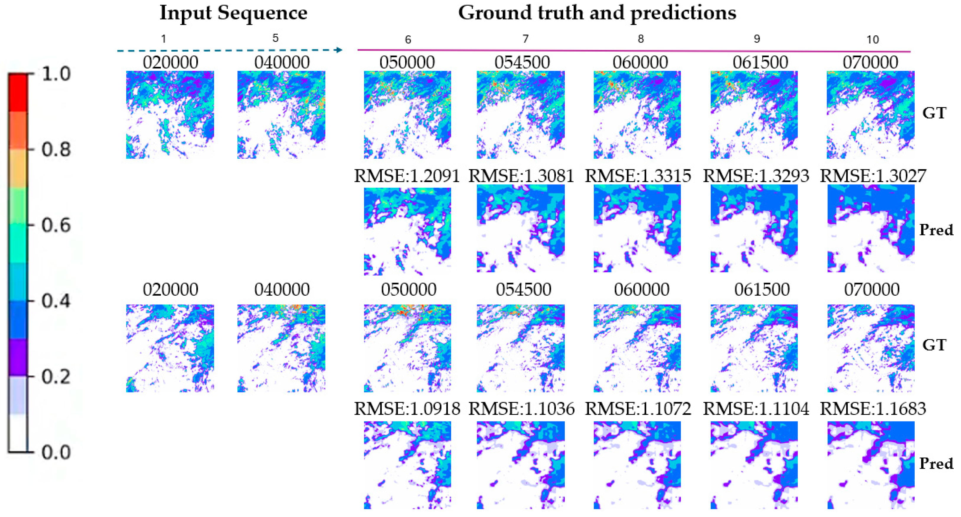
In conclusion, the prediction of COT is influenced by factors such as time interval, input sequence length, and output sequence length. The prediction performance improves with a more extended input sequence, shorter time intervals, and when the predicted frames are closer to the input frames in time. Figure 8, Figure 9, Figure 10 and Figure 11 show the COT prediction results by CPM for two randomly selected days under different input sequence lengths. The title of each figure indicates the UTC (HH: MM: SS).

The experimental results indicate that CPM outperforms other benchmark prediction models, with an RMSE of 0.878, MAE of 0.560, SSIM of 0.5179, and PSNR of 29.9403. Both RMSE and MAE are lower than those of SimVP and ConvLSTM, while SSIM and PSNR are higher than those of SimVP and ConvLSTM. Due to the incorporation of the time embedding module and the utilization of Charbonnier Loss and Edge Loss as loss functions, CPM outperforms the video prediction model SimVP in various metrics. Additionally, through the analysis of CPM prediction results under different input sequence lengths, we found that the length of the input and output sequence and the time interval between adjacent frames both affect the prediction results of COT.

6. Conclusions

In this paper, we developed a CNN-based CM4CR algorithm for daytime COT retrieval. The model utilizes FY-4A channel data, geographic data, and CLP products as inputs, with COT observations derived from multi-point averaging by CALIPSO as the ground truth values. We perform single-point matching within the constrained spatiotemporal range by associating selected points with the nearest CALIPSO scanning points. Subsequently, 9 × 9 grid slices centered at the matching points are generated for CNN training. The experimental results demonstrate that our model achieves satisfactory performance on the test set, with an RMSE of 1.26, R² of 0.75, and MAE of 0.86.

Upon retrieving COT values, we further investigated COT prediction and found that it is essentially a spatiotemporal sequence prediction task. Therefore, we proposed a COT prediction method based on a video prediction model, CPM. We compared CPM with other benchmark models. The experimental results demonstrate that our model exhibits superior prediction performance, with an RMSE of 0.878, MAE of 0.560, SSIM of 0.5179, and PSNR of 29.9403. The RMSE and MAE are lower than other benchmark models, while SSIM and PSNR are higher. Meanwhile, through the analysis of CPM prediction results under different input sequence lengths, we found that the length of the input and output sequence and the time interval between adjacent frames both affect the prediction results of COT. The prediction performance improves with a more extended input sequence, shorter time intervals, and when the predicted frames are closer in time to the input frames.

However, current satellite remote sensing efforts primarily focus on studying daytime cloud microphysical products. Extracting nighttime cloud optical thickness (COT) products remains a significant challenge, including during twilight. Additionally, due to data quality issues, such as local data gaps and irregular time intervals between data points, there still exists significant research space for capturing COT detail information and reducing the accumulation of errors during multi-sequence forecasting.

References

1. Khain, A.; Rosenfeld, D.; Pokrovsky, A. Aerosol impact on precipitation from convective clouds. In Measuring Precipitation from Space: EURAINSAT and the Future; Springer: Dordrecht, The Netherlands, 2007; pp. 421–434. [Google Scholar]
2. Jensen, E.J.; Kinne, S.; Toon, O.B. Tropical cirrus cloud radiative forcing: Sensitivity studies. Geophys. Res. Lett. 1994, 21, 2023–2026. [Google Scholar] [CrossRef]
3. Roeckner, E.; Schlese, U.; Biercamp, J.; Loewe, P. Cloud optical depth feedbacks and climate modelling. Nature 1987, 329, 138–140. [Google Scholar] [CrossRef]
4. Mitchell, J.F.B.; Senior, C.A.; Ingram, W.J. C02 and climate: A missing feedback? Nature 1989, 341, 132–134. [Google Scholar] [CrossRef]
5. Stephens, G.L.; Webster, P.J. Clouds and climate: Sensitivity of simple systems. J. Atmos. Sci. 1981, 38, 235–247. [Google Scholar] [CrossRef]
6. Nakajima, T.Y.; Uchiyama, A.; Takamura, T.; Nakajima, T. Comparisons of warm cloud properties obtained from satellite, ground, and aircraft measurements during APEX intensive observation period in 2000 and 2001. J. Meteorol. Soc. Japan Ser. II 2005, 83, 1085–1095. [Google Scholar] [CrossRef]
7. Gao, Z.; Shi, X.; Wang, H.; Yeung, D.-Y.; Woo, W.; Wong, W.-K. Deep learning and the weather forecasting problem: Precipitation nowcasting. In Deep Learning for the Earth Sciences: A Comprehensive Approach to Remote Sensing, Climate Science, and Geosciences; John Wiley & Sons, Ltd.: Chichester, UK, 2021; pp. 218–239. [Google Scholar]
8. Chen, S.; Zhang, X.; Shao, D.; Shu, X. SASTA-Net: Self-attention spatiotemporal adversarial network for typhoon prediction. J. Electron. Imaging 2022, 31, 053020. [Google Scholar] [CrossRef]
9. Wang, R.; Teng, D.; Yu, W.; Zhang, X.; Zhu, J. Improvement and Application of a GAN Model for Time Series Image Prediction—A Case Study of Time Series Satellite Cloud Images. Remote Sens. 2022, 14, 5518. [Google Scholar] [CrossRef]
10. Letu, H.; Yang, K.; Nakajima, T.Y.; Ishimoto, H. High-resolution retrieval of cloud microphysical properties and surface solar radiation using Himawari-8/AHI next-generation geostationary satellite. Remote Sens. Environ. 2020, 239, 111583. [Google Scholar] [CrossRef]
11. Liu, C.; Song, Y.; Zhou, G.; Teng, S.; Li, B.; Xu, N.; Lu, F.; Zhang, P. A cloud optical and microphysical property product for the advanced geosynchronous radiation imager onboard China’s Fengyun-4 satellites: The first version. Atmos. Ocean. Sci. Lett. 2023, 16, 100337. [Google Scholar] [CrossRef]
12. Kox, S.; Bugliaro, L.; Ostler, A. Retrieval of cirrus cloud optical thickness and top altitude from geostationary remote sensing. Atmos. Meas. Tech. 2014, 7, 3233–3246. [Google Scholar] [CrossRef]
13. Minnis, P.; Hong, G.; Sun-Mack, S.; Smith, W.L.; Chen, Y.; Miller, S.D. Estimating nocturnal opaque ice cloud optical depth from MODIS multispectral infrared radiances using a neural network method. J. Geophys. Res. Atmos. 2016, 121, 4907–4932. [Google Scholar] [CrossRef]
14. Wang, X.; Iwabuchi, H.; Yamashita, T. Cloud identification and property retrieval from Himawari-8 infrared measurements via a deep neural network. Remote Sens. Environ. 2022, 275, 113026. [Google Scholar] [CrossRef]
15. Wang, Q.; Zhou, C.; Zhuge, X.; Liu, C.; Weng, F.; Wang, M. Retrieval of cloud properties from thermal infrared radiometry using convolutional neural network. Remote Sens. Environ. 2022, 278, 113079. [Google Scholar] [CrossRef]
16. Li, J.; Zhang, F.; Li, W.; Tong, X.; Pan, B.; Li, J.; Lin, H.; Letu, H.; Mustafa, F. Transfer-learning-based approach to retrieve the cloud properties using diverse remote sensing datasets. In Proceedings of the IEEE Transactions on Geoscience and Remote Sensing, Pasadena, CA, USA, 13 October 2023. [Google Scholar]
17. Curran, R.J.; Wu, M.L.C. Skylab near-infrared observations of clouds indicating supercooled liquid water droplets. J. Atmos. Sci. 1982, 39, 635–647. [Google Scholar] [CrossRef]
18. Platnick, S.; King, M.D.; Ackerman, S.A.; Menzel, W.P.; Baum, B.A.; Riédi, J.C.; Frey, R.A. The MODIS cloud products: Algorithms and examples from Terra. IEEE Trans. Geosci. Remote Sens. 2003, 41, 459–473. [Google Scholar] [CrossRef]
19. Letu, H.; Nagao, T.M.; Nakajima, T.Y.; Riedi, J.; Ishimoto, H.; Baran, A.J.; Shang, H.; Sekiguchi, M.; Kikuchi, M. Ice cloud properties from Himawari-8/AHI next-generation geostationary satellite: Capability of the AHI to monitor the DC cloud generation process. IEEE Trans. Geosci. Remote Sens. 2018, 57, 3229–3239. [Google Scholar] [CrossRef]
20. Greenwald, T.J.; Pierce, R.B.; Schaack, T.; Otkin, J.A.; Rogal, M.; Bah, K.; Lenzen, A.J.; Nelson, J.P.; Li, J.; Huang, H.-L. Real-time simulation of the GOES-R ABI for user readiness and product evaluation. Bull. Am. Meteorol. Soc. 2016, 97, 245–261. [Google Scholar] [CrossRef]
21. Woo, S.; Park, J.; Lee, J.Y.; Kweon, I.-S. Cbam: Convolutional block attention module. In Proceedings of the European Conference on Computer Vision (ECCV), Munich, Germany, 8–14 September 2018; pp. 3–19. [Google Scholar]
22. Gao, Z.; Tan, C.; Wu, L.; Li, S.Z. Simvp: Simpler yet better video prediction. In Proceedings of the IEEE/CVF Conference on Computer Vision and Pattern Recognition, New Orleans, LA, USA, 18–24 June 2022; pp. 3170–3180. [Google Scholar]
23. Seo, M.; Lee, H.; Kim, D.; Seo, J. Implicit stacked autoregressive model for video prediction. arXiv 2023, arXiv:2303.07849. [Google Scholar]
24. Oprea, S.; Martinez-Gonzalez, P.; Garcia-Garcia, A.; Castro-Vargas, J.A.; Orts-Escolano, S.; Garcia-Rodriguez, J.; Argyros, A. A review on deep learning techniques for video prediction. IEEE Trans. Pattern Anal. Mach. Intell. 2020, 44, 2806–2826. [Google Scholar] [CrossRef]
25. Hsieh, J.T.; Liu, B.; Huang, D.A.; Li, F.-F.; Niebles, J.C. Learning to decompose and disentangle representations for video prediction. In Proceedings of the 32nd Conference on Neural Information Processing Systems (NeurIPS 2018), Montreal, QC, Canada, 3–8 December 2018; Volume 31. [Google Scholar]
26. Byeon, W.; Wang, Q.; Srivastava, R.K.; Koumoutsakos, P. Contextvp: Fully context-aware video prediction. In Proceedings of the European Conference on Computer Vision (ECCV), Munich, Germany, 8–14 September 2018; pp. 753–769. [Google Scholar]
27. Zamir, S.W.; Arora, A.; Khan, S.; Hayat, M.; Khan, F.S.; Yang, M.-H.; Shao, L. Multi-stage progressive image restoration. In Proceedings of the IEEE/CVF Conference on Computer Vision and Pattern Recognition, Nashville, TN, USA, 20–25 June 2021; pp. 14821–14831. [Google Scholar]
28. Barnard, J.C.; Long, C.N. A simple empirical equation to calculate cloud optical thickness using shortwave broadband measurements. J. Appl. Meteorol. 2004, 43, 1057–1066. [Google Scholar] [CrossRef]
29. Kikuchi, N.; Nakajima, T.; Kumagai, H.; Kamei, A.; Nakamura, R.; Nakajima, T.Y. Cloud optical thickness and effective particle radius derived from transmitted solar radiation measurements: Comparison with cloud radar observations. J. Geophys. Res. Atmos. 2006, 111, D07205. [Google Scholar] [CrossRef]
30. Gong, K.; Ye, D.L.; Ge, C.H. A method for geostationary meteorological satellite cloud image prediction based on motion vector. J. Image Graph. 2000, 50, 5. [Google Scholar]
31. Lorenz, E.; Hammer, A.; Heinemann, D. Short term forecasting of solar radiation based on satellite data. In EUROSUN2004 (ISES Europe Solar Congress); PSE Instruments GmbH, Solar Info Center: Freiburg, Germany, 2004. [Google Scholar]
32. Yang, J.; Lv, W.T.; Ma, Y.; Yao, W.; Li, Q. An automatic groundbased cloud detection method based on local threshold interpolation. Acta Meteorol. Sin. 2010, 68, 1007–1017. [Google Scholar]
33. Shi, X.; Chen, Z.; Wang, H.; Yeung, D.-Y. Convolutional LSTM network: A machine learning approach for precipitation nowcasting. In Proceedings of the Advances in Neural Information Processing Systems 28: Annual Conference on Neural Information Processing Systems 2015, Montreal, QC, Canada, 7–12 December 2015; Volume 28. [Google Scholar]
34. Shi, X.; Gao, Z.; Lausen, L.; Yeung, D.-Y. Deep learning for precipitation nowcasting: A benchmark and a new model. In Proceedings of the 31st Conference on Neural Information Processing Systems (NIPS 2017), Long Beach, CA, USA, 4–9 December 2017; Volume 30. [Google Scholar]
35. Wang, Y.; Long, M.; Wang, J.; Gao, Z.; Yu, P.S. Predrnn: Recurrent neural networks for predictive learning using spatiotemporal lstms. In Proceedings of the 31st Conference on Neural Information Processing Systems (NIPS 2017), Long Beach, CA, USA, 4–9 December 2017; Volume 30. [Google Scholar]
36. Requena-Mesa, C.; Benson, V.; Reichstein, M.; Runge, J.; Denzler, J. EarthNet2021: A large-scale dataset and challenge for Earth surface forecasting as a guided video prediction task. In Proceedings of the IEEE/CVF Conference on Computer Vision and Pattern Recognition, Nashville, TN, USA, 20–25 June 2021; pp. 1132–1142. [Google Scholar]
37. Yu, Z.; Ma, S.; Han, D.; Li, G.; Yan, W.; Liu, J. Physical and optical properties of clouds in the southwest Vortex from FY-4A cloud retrievals. J. Appl. Meteorol. Climatol. 2022, 61, 1123–1138. [Google Scholar] [CrossRef]
38. Lai, R.; Teng, S.; Yi, B.; Letu, H.; Min, M.; Tang, S.; Liu, C. Comparison of cloud properties from Himawari-8 and FengYun-4A geostationary satellite radiometers with MODIS cloud retrievals. Remote Sens. 2019, 11, 1703. [Google Scholar] [CrossRef]
39. Krebs, W.; Mannstein, H.; Bugliaro, L.; Mayer, B. A new day-and night-time Meteosat Second Generation Cirrus Detection Algorithm MeCiDA. Atmos. Chem. Phys. 2007, 7, 6145–6159. [Google Scholar] [CrossRef]
40. Li, Q.; Sun, X.; Wang, X. Reliability evaluation of the joint observation of cloud top height by FY-4A and Himawari-8. Remote Sens. 2021, 13, 3851. [Google Scholar] [CrossRef]
41. Xu, X.; Zeng, Y.; Yu, X.; Liu, G.; Yue, Z.; Dai, J.; Feng, Q.; Liu, P.; Wang, J.; Zhu, Y. Identification of Supercooled Cloud Water by FY-4A Satellite and Validation by CALIPSO and Airborne Detection. Remote Sens. 2022, 15, 126. [Google Scholar] [CrossRef]
42. Wu, W.; Liu, Y.; Jensen, M.P.; Toto, T.; Foster, M.J.; Long, C.N. A Comparison of Multiscale Variations of Decade-Long Cloud Fractions from Six Different Platforms over the Southern Great Plains in the United States. Geophys. Res. Atmos. 2014, 119, 3438–3459. [Google Scholar] [CrossRef]
43. Zhang, D.; Luo, T.; Liu, D.; Wang, Z. Spatial scales of altocumulus clouds observed with collocated CALIPSO and CloudSat measurements. Atmos. Res. 2014, 149, 58–69. [Google Scholar] [CrossRef]
44. Hendrycks, D.; Gimpel, K. Gaussian Error Linear Units (GELUs). arXiv 2016, arXiv:1606.08415. [Google Scholar] [CrossRef]
45. Vaswani, A.; Shazeer, N.; Parmar, N.; Uszkoreit, J.; Jones, L.; Gomez, A.N.; Kaiser, Ł.; Polosukhin, I. Attention is all you need. In Proceedings of the 31st International Conference on Neural Information Processing Systems (NIPS 2017), Long Beach, CA, USA, 4–9 December 2017; pp. 6000–6010. [Google Scholar]
46. Guo, M.H.; Lu, C.Z.; Liu, Z.N.; Cheng, M.M.; Hu, S.M. Visual attention network. Comput. Vis. Media 2023, 9, 733–752. [Google Scholar] [CrossRef]
Figure 1. Summary of research process.
Remotesensing 16 02136 g001
Figure 2. Architecture of CM4CR.
Remotesensing 16 02136 g002
Figure 3. Architecture of CPM.
Remotesensing 16 02136 g003
Figure 4. Histogram of COT distribution in the year 2021.
Remotesensing 16 02136 g004
Figure 5. Scatter density plot of true COT and predicted COT on the test set (a) and the distribution histograms of true COT and predicted COT (b).
Remotesensing 16 02136 g005
Figure 6. FY-4A full-disk COT results during daytime. COT retrieval results based on the CNN model from 2:00~8:00 UTC on May 17, 2022. The black part is daytime or invalid observation, and the white part is the no-cloud area (ag).
Remotesensing 16 02136 g006
Figure 7. Scatter plot of results for three models on the test set (10,000 randomly selected points). (a) CPM. (b) SimVP. (c) ConvLSTM.
Remotesensing 16 02136 g007
Figure 8. Prediction results of CPM when T = 10 and T′ = 1. The RMSE in the figure is calculated after denormalization.
Remotesensing 16 02136 g008
Figure 9. Prediction results of CPM when T = 8 and T′ = 3. The RMSE in the figure is calculated after denormalization.
Remotesensing 16 02136 g009
Figure 10. Prediction results of CPM when T = 8 and T′ = 2. The RMSE in the figure is calculated after denormalization.
Remotesensing 16 02136 g010
Figure 11. Prediction results of CPM when T = 5 and T′ = 5. The RMSE in the figure is calculated after denormalization.
Remotesensing 16 02136 g011