Article

A Low-Cost 3D SLAM System Integration of Autonomous Exploration Based on Fast-ICP Enhanced LiDAR-Inertial Odometry

1
Electronic Information School, Wuhan University, Wuhan 430072, China
2
The State Key Laboratory of Information Engineering in Surveying, Mapping and Remote Sensing, Wuhan University, Wuhan 430072, China
3
Intellectual Computing Laboratory for Cultural Heritage, Wuhan University, Wuhan 430072, China
*
Author to whom correspondence should be addressed.
Remote Sens. 2024, 16(11), 1979; https://doi.org/10.3390/rs16111979
Submission received: 25 March 2024 / Revised: 24 May 2024 / Accepted: 24 May 2024 / Published: 30 May 2024

Abstract

:
Advancements in robotics and mapping technology have spotlighted the development of Simultaneous Localization and Mapping (SLAM) systems as a key research area. However, the high cost of advanced SLAM systems poses a significant barrier to research and development in the field, while many low-cost SLAM systems, operating under resource constraints, fail to achieve high-precision real-time mapping and localization, rendering them unsuitable for practical applications. This paper introduces a cost-effective SLAM system design that maintains high performance while significantly reducing costs. Our approach utilizes economical components and efficient algorithms, addressing the high-cost barrier in the field. First, we developed a robust robotic platform based on a traditional four-wheeled vehicle structure, enhancing flexibility and load capacity. Then, we adapted the SLAM algorithm using the LiDAR-inertial Odometry framework coupled with the Fast Iterative Closest Point (ICP) algorithm to balance accuracy and real-time performance. Finally, we integrated the 3D multi-goal Rapidly exploring Random Tree (RRT) algorithm with Nonlinear Model Predictive Control (NMPC) for autonomous exploration in complex environments. Comprehensive experimental results confirm the system’s capability for real-time, autonomous navigation and mapping in intricate indoor settings, rivaling more expensive SLAM systems in accuracy and efficiency at a lower cost. Our research results are published as open access, facilitating greater accessibility and collaboration.

1. Introduction

In the interdisciplinary realm of robotics, computer vision and artificial intelligence, Simultaneous Localization and Mapping (SLAM) [1] stands out as a hot topic technology that enables autonomous systems to navigate and understand their surroundings. SLAM’s principle entails mapping an uncharted environment and concurrently monitoring the agent’s position within this space [2]. This technology is important for many applications, including self-driving cars [3,4,5] and augmented reality [6,7,8], making SLAM a major focus in the development of smart, self-guiding machines.
The development of SLAM technology is rapid, driven by continuous advancements in computational power, algorithmic efficiency, and sensor technology. Over the years, various SLAM solutions have been developed, each employing distinct methodologies and technological advancements to address the challenges of mapping and localization. Early approaches [9,10,11] relied heavily on expensive and high-precision sensors, like lasers, to achieve detailed environmental mapping and accurate localization. These systems, while effective, were often limited by their high costs and substantial computational requirements, which deviated from the original intention of SLAM technology. Additionally, early SLAM systems exhibited limited adaptability to dynamic environments and were susceptible to interference, necessitating high-quality and high-performance LiDAR sensors. This indirectly escalated the operational costs of SLAM systems and restricted their widespread adoption in various application scenarios.
One of the recent advancements in SLAM has seen the integration of visual SLAM (VSLAM) techniques [12,13,14,15,16,17], which relies on camera images to perform localization and mapping tasks. While VSLAM systems reduced the reliance on costly sensors, they introduced new challenges, particularly in terms of real-time processing capabilities. Processing high-resolution video feeds in real-time requires significant computational power, which can still lead to high system costs [14]. Furthermore, visual SLAM systems can struggle in low-light conditions or environments with repetitive textures, leading to decreased reliability and accuracy, which adversely affects the stability of low-cost SLAM systems.
Recently, solid-state LiDARs have gained prominence as a primary trend in LiDAR development due to advancements in technology, especially in micro-electro-mechanical systems (MEMS) [18] and rotating prisms [19]. These LiDARs offer improved reliability and cost-effectiveness, as they eliminate the need for rotating mechanical parts, resulting in a more compact design. Their lightweight and high-performance characteristics enable solid-state LiDARs to deliver accurate 3D measurements over long ranges, making them ideal for autonomous vehicles, industrial robots, and drones that require precise 3D mapping in complex or challenging environments. Solid-state LiDARs are becoming critical for enabling intelligent systems and integrating seamlessly into lightweight, low-cost SLAM systems. However, due to the high resolution of solid-state LiDAR, its scans typically contain a significant number of feature points (ranging from thousands to tens of thousands). Processing the data from the IMU combined with the numerous feature points can overwhelm low-cost edge computing systems. Furthermore, the scan frequency often exceeds that of the IMU, resulting in motion distortion, which makes registration challenging for LiDAR-Inertial Odometry (LIO) based LiDAR SLAM algorithms [20].
Another critical issue facing contemporary SLAM systems is how to incorporate autonomous exploration modules. Autonomous exploration refers to a system’s ability to independently navigate and collect information from its environment under the guidance of its own decision-making processes, widely applied in robotic exploration and mapping in unknown complex environments [21]. Early exploration algorithms, such as Frontier-Based Exploration [22] and Greedy Search [23], prioritized discovering unexplored regions to improve map coverage but tended to get trapped in local optima in complex terrains. Additionally, they faced real-time decision-making challenges due to computational limitations and an inability to effectively handle dynamic environmental changes.
Recent advances have combined exploration with SLAM, improving how autonomous systems understand and adapt to their surroundings [21,24,25]. Despite these advancements, a significant limitation remains the traditional focus on 2D exploration strategies, primarily designed for ground-based robots. This emphasis limits SLAM systems’ ability to autonomously reconstruct 3D environments in real-world settings [26], which are intrinsically three-dimensional and complex.
Addressing these challenges, this paper proposes a novel, cost-effective SLAM system that balances cost, accuracy, and real-time performance. The primary contributions of our work are threefold:
  • We developed a low-cost mobile robot SLAM system, significantly reducing manufacturing costs and enhancing system performance and 3D exploration capabilities through careful design of the robot’s structure and selection of high-performing yet affordably priced sensors and components.
  • We successfully deployed an integrated LiDAR and IMU fusion SLAM algorithm framework with 3D autonomous exploration capabilities on the robot and conducted targeted optimizations for this algorithm based on our robot, achieving superior performance on our hardware platform.
  • Our research findings have been made available as open-source, providing a high-performance solution for SLAM research under budget constraints and facilitating the wider adoption and application of advanced SLAM technologies.
The structure of the remaining sections in this paper is delineated as follows: Section 2 delves into the technical background of existing SLAM solutions, highlighting their strengths and delineating their limitations in terms of cost and real-time performance. Section 3 describes our methodology for developing a cost-effective SLAM system, focusing on hardware design, algorithm development and SLAM system optimizations. Section 4 presents our experimental results, demonstrating the effectiveness of our system in various scenarios. Section 5 discusses these methods in the broader context of SLAM research, summing up the advantages and disadvantages of the design. Finally, Section 6 concludes the paper with a summary of our contributions and outlines directions for further research.

2. Related Work

2.1. SLAM

The framework of SLAM systems generally consists of five parts: sensor data acquisition and processing, front-end odometry (indicated within the dashed red boundary in Figure 1), back-end optimization (indicated within the dashed blue boundary in Figure 1), loop closure detection, and map construction. Initially, LiDAR or visual sensors collect data, which is then roughly estimated for pose transformations between data frames by the front-end odometry. This is followed by global trajectory optimization through the back-end optimizer, after which precise poses are used for map construction. During the operation of SLAM, loop closure detection continuously identifies scenes traversed by the robot to eliminate cumulative errors.
Depending on the type of sensor used, mainstream SLAM systems are typically categorized into single-sensor SLAM, such as LiDAR-based [27,28,29,30] and vision-based [12,13,14,15,16], and multi-sensor fusion SLAM techniques [31,32,33,34,35], integrating various sensors to enhance SLAM performance. Visual SLAM systems, favored for their rich information acquisition, lightweight sensors, and low cost, face challenges due to their sensitivity to light, substantial accuracy variance under varying illumination, and extensive image data processing that compromises real-time performance.
LiDAR-based SLAM systems, on the other hand, effectively address these issues. LiDAR can directly measure distances with minimal influence from ambient light, providing more accurate environmental perception and capturing the spatial location and shape information of objects while delivering data that is straightforward to process. This foundation enables LiDAR SLAM systems to be more real-time, stable, and reliable. From initial 2D mapping techniques to complex 3D modeling methods, LiDAR SLAM has made significant advancements and has become a hot technology in robotics and autonomous driving, offering high-resolution, three-dimensional environmental perception and mapping capabilities. In 2012, A. Geiger, P. Lenz, and R. Urtasun introduced the KITTI Vision Benchmark Suite, followed by the release of the KITTI public dataset in 2013, intended for building and evaluating SLAM algorithms. The KITTI dataset includes real image and three-dimensional LiDAR data collected from urban, rural, and highway scenes, providing diverse environmental data for the development of 3D LiDAR SLAM algorithms, thereby accelerating their advancement.
Early 3D LiDAR SLAM algorithms heavily relied on The Iterative Closest Point (ICP) for point cloud matching and map construction. The ICP algorithm was initially proposed by Besl and McKay in 1992 [36]. It is designed to align two sets of point cloud data in three-dimensional space. The ICP algorithm seeks the optimal rigid-body transformation (including rotation and translation) through an iterative process, aligning one point cloud with another to minimize the distance between points across the two sets. The core advantage of the ICP algorithm lies in its simplicity and wide applicability, making it a crucial tool in fields such as 3D scanning and robotic vision. Over time, researchers have made various enhancements to the ICP algorithm to improve its robustness and efficiency. For instance, the introduction of a multi-resolution strategy to accelerate the alignment process [37]. In 2015, Pomerleau, Colas, and Siegwart discussed various ICP algorithms and their applications across different robotic platforms, environments, and tasks [38]. Although the ICP algorithm has been widely used for registering LIDAR scan data, its efficiency issues persist. The authors of [39] propose a method to accelerate the obstacle detection process by directly monitoring outliers detected after ICP matching, incorporating an improved ICP implementation within the SLAMICP library.
With the growing demand for more complex spatial understanding, the simple ICP algorithm, due to its high computational load and long processing time, no longer meets the real-time requirements of SLAM algorithms. The shift towards 3D LiDAR SLAM is increasingly evident, highlighted by the introduction of pioneering frameworks such as LOAM (LiDAR Odometry and Mapping) [40] and its variants [29,30], which strike a good balance between real-time processing and mapping accuracy. Despite these advancements, LiDAR SLAM still faces challenges, especially in dynamic environments and during extended operations, where cumulative errors can pose significant obstacles. Moreover, the typically high expenses associated with LiDAR SLAM systems, along with the significant computational resource demands of LOAM, present challenges for the broader adoption of LiDAR SLAM systems.
LiDAR-inertial odometry [20], which incorporates Inertial Measurement Units (IMUs), bolsters autonomous navigation systems by offering a synergy between LiDAR’s detailed 3D environmental mappings through laser scanning and the IMU’s motion data, including acceleration and rotational changes. This fusion enhances positioning and mapping with greater accuracy and robustness, compensating for the inherent limitations of each sensor type. Furthermore, while the prevalent LiDAR Odometry and Mapping (LOAM) [28] framework somewhat improves 3D LiDAR SLAM capabilities, its reliance on high-precision LiDAR and susceptibility to dynamic objects and environmental variations poses significant challenges.
As sensor technology progresses and hardware capabilities improve, there is a growing trend in the volume of data that SLAM systems must process. Consequently, there is a gradual increase in the demand for computational resources by algorithms. In this context, the challenge of ensuring algorithm performance and system stability while effectively controlling costs has become a significant concern in the development of SLAM technology. Faced with increasingly complex application scenarios and expanding data processing requirements, exploring more cost-effective computational methods and optimizing algorithms to reduce dependence on high-performance hardware holds practical significance for swiftly adapting to the ongoing evolution in the SLAM domain.

2.2. Autonomous Exploration

Robotic autonomous exploration enables robots to independently navigate unknown environments without human intervention, relying on their own sensors, algorithms, and decision-making capabilities. This process involves several steps, including environmental perception, map construction, path planning, and decision execution. While autonomous exploration is often considered a distinct research area akin to SLAM, recent years have seen a growing interest in integrating autonomous exploration into SLAM systems, demonstrating heightened potential in terms of robotic intelligence and integration [41].
Common autonomous exploration algorithms employ a breadth-first search [42] strategy to identify the nearest boundary points to the robot, followed by path planning to navigate toward these points. If a boundary point is reached or deemed unreachable within a certain period, the algorithm proceeds to the next search cycle, repeating this process until a complete environmental map is obtained. While effective in many settings, breadth-first-based autonomous exploration algorithms can lead to frequent changes in the robot’s movement and an excessive increase in data volume, placing significant strain on the computational resources of resource-constrained mobile robots.
RRT Exploration [43,44], which is based on the Rapidly exploring Random Tree path planning algorithm [26], offers significant improvements in search efficiency and adaptability to dynamic environments over traditional breadth-first search strategies [45]. It begins from an initial node and randomly selects points within the exploration area, extending new nodes towards these points in the absence of obstacles and incorporating them into the tree. This process enables RRT to quickly cover the entire exploration space, generating paths from the start to any point. However, both traditional exploration algorithms and RRT Exploration are generally confined to 2D operations using Scan LiDAR, which limits their effectiveness in 3D environments.
The 3D RRT algorithm [46], an extension of the traditional RRT, represents a significant advancement in the field of autonomous exploration in three-dimensional spaces, specifically tailored for 3D path planning challenges. It employs heuristic strategies to guide the random selection of target points across the 3D space, expanding nodes across all three dimensions (x, y, and z). Following the addition of an endpoint, 3D RRT conducts collision checks to ensure that the path from the nearest node to the new node does not intersect with any obstacles. Upon passing the collision test, the new node is integrated into the tree connected to the nearest node by an edge. The 3D RRT framework efficiently explores and generates paths from the starting point to the endpoint within 3D spaces, rapidly adapting to complex environments without demanding excessive computational resources, offering a notable performance advantage over other more costly and complex autonomous exploration systems. Although the 3D RRT algorithm represents a significant advancement in enhancing autonomous exploration within three-dimensional spaces, its wider implementation is constrained by considerations of cost, computational resource allocation, and practical deployment challenges. Similar autonomous exploration algorithms like [47] that operate in 3D spaces require high-performance computational capabilities for constructing three-dimensional maps and planning exploration paths, potentially leading to increased operational costs, especially for extensive or prolonged tasks.
Furthermore, the resource limitations of mobile robotic platforms often restrict the extent to which such advanced algorithms can be implemented without compromising other essential functions. Balancing the requirements of sophisticated autonomous exploration algorithms like 3D RRT with the practicalities of cost and computational efficiency remains a key challenge, necessitating innovative solutions to render these technologies more accessible and feasible for broad application.

3. Method

3.1. Cost-Effective Hardware Design

In the hardware design of SLAM systems, prioritizing cost efficiency is paramount, yet not at the expense of performance and reliability. Currently, there are two main solutions for ground robots: the first approach utilizes a three-wheeled design [48] consisting of two active drive wheels and one or more passive support wheels (similar to a robotic vacuum), facilitating simple steering and navigation in confined spaces. Although this design simplifies the control system, it also limits dynamic stability and load-bearing capacity. The alternative solution involves a four-wheeled vehicle with Mecanum wheels [49], which allows for omnidirectional motion. Vehicles equipped with Mecanum wheels offer enhanced maneuverability and superior load-bearing capabilities. Yet, they are susceptible to odometry drift from slippage, and their unique structure and control mechanisms result in higher maintenance costs.
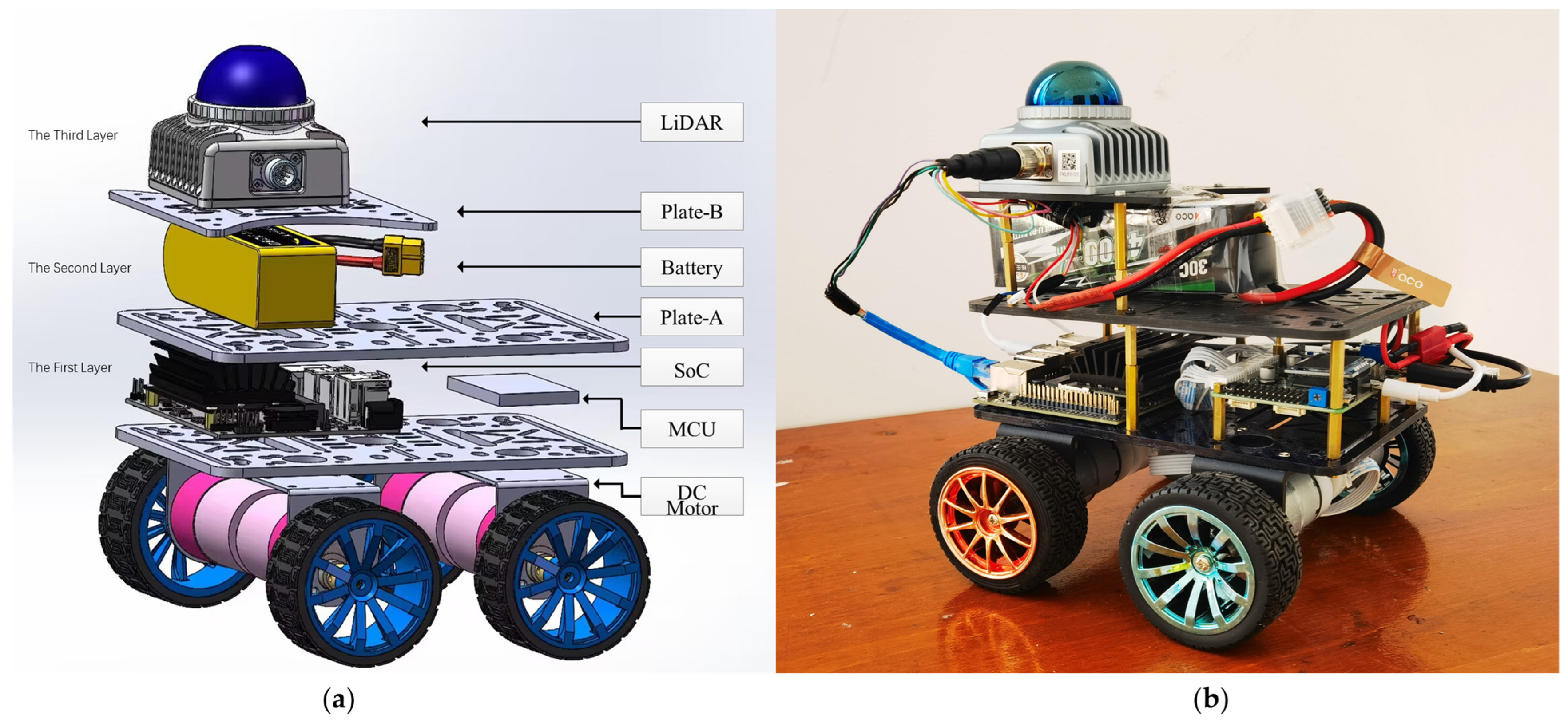
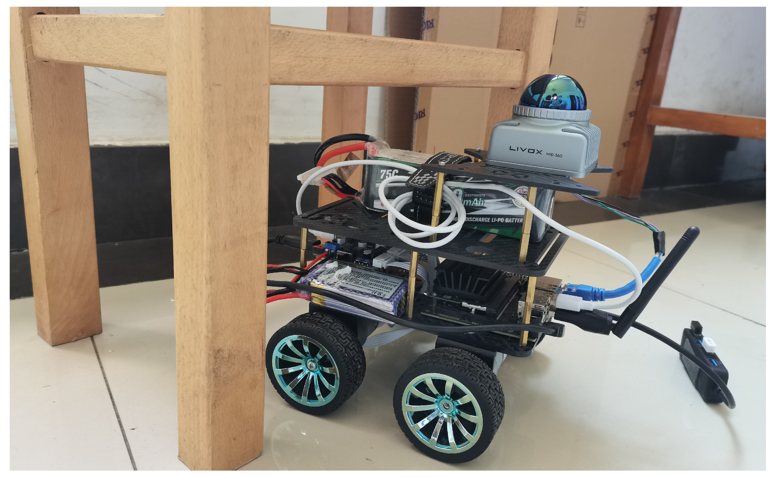
Addressing the limitations of existing solutions, this paper draws inspiration from automotive structures, adopting a four-wheeled rubber tire and custom carbon plate chassis to enhance the vehicle’s stability and load capacity through the superior ground traction of rubber tires and the high structural integrity of carbon plates. Departing from the traditional Ackermann steering geometry found in automobiles, this vehicle incorporates four fixed DC geared motors, a configuration that simplifies the mechanical structure and reduces component count, thereby significantly lowering manufacturing and maintenance costs while ensuring agility and stability. The ability to independently control the direction and speed of each motor endows the system with effective spot-turning capabilities, essential for meticulous steering and path planning in restricted areas. The base plate’s design features a 17:11 aspect ratio and a triple-layered structure, expanding sensor installation space while optimizing body volume and weight to achieve a balance between high performance and minimized cost and size. The result is shown in Figure 2, and The specific parameters of the radar sensors used in this SLAM system are shown in Table 1.
Benefiting from the recent cost reduction in LiDAR and single-board computers, our system integrates high-performance sensors within a compact design. The main computing unit employs the Jetson Nano ($129) paired with the MID-360 ($556.44), forming the core of our system. This cost-efficient configuration facilitates the deployment of advanced SLAM capabilities in budget-constrained applications, thereby democratizing sophisticated navigation and mapping technologies. The total expenses for the hardware system can be seen in Table 2.

3.2. LiDAR-Inertial Odometry Using Fast-ICP

3.2.1. SLAM Framework Design

Due to the need for localization in high-dynamic environments, to maintain computational efficiency, and to mitigate sensor noise and data ambiguity, 3D LiDAR SLAM struggles to ensure real-time performance at low cost, especially traditional odometry frameworks that are unable to allow robust navigation and mapping. So, we propose an efficient method to ensure robustness and balance performance with cost-effectiveness.
We adopt the high-performance LiDAR-inertial odometry framework FAST-LIO in [31] as our foundation to build up our SLAM system. Different from [31], we incorporate an ICP optimization module into it [36,37] that utilizes KD-trees for fast nearest-neighbor searches and employs the Gauss–Newton iterative method, as illustrated in Figure 3 (on the right side). Our approach comprises four main stages. Initially, the system collects point cloud and IMU data from the Mid-360 LiDAR and preprocesses the LiDAR data. Subsequently, extracted features are fed into the state estimation module for initial state estimation and vehicle localization. Following that, the Fast ICP algorithm [37] precisely aligns the current point cloud frame with the previous one, optimizing state estimation and setting the stage for precise mapping. Ultimately, the map is updated using the optimized state estimates, continuously integrating new point cloud data into the existing map for real-time maintenance. The overview of our workflow is shown in Figure 3.

3.2.2. State Estimation Based on State Iterated Kalman Filter

State estimation plays a pivotal role in SLAM, involving the determination of an object’s orientation and position within a given environment. Traditional state estimation algorithms, which rely on feature extraction and matching, excel in environments with distinct landmarks but falter in dynamic or feature-sparse areas owing to occlusion risks and extensive computational demands. Some works directly enhance SLAM with real-time 3D mapping via LiDAR yet falter in challenging conditions or under computational constraints due to reliance on high-quality data and intensive processing [28,29,30].
We choose to employ a tightly coupled iterated Kalman filter [35,50] for enhanced State estimation within our SLAM system. This filter is particularly adept at handling the uncertainties and dynamics of real-world environments by cohesively integrating sensor measurements. This method not only addresses the challenges of occlusions and feature scarcity but also ensures robust performance despite computational constraints. This seamless integration of sensor data, particularly from LiDAR and IMU, forms the basis for our approach to handling the high-frequency data and temporal alignment challenges inherent in real-time SLAM applications.
Given the original LiDAR’s high sampling rate, processing each point in real-time is impractical. Therefore, we accumulate these points over a period, and an accumulated set of points before collective processing is referred to as a scan. Following each scan’s preprocessing, the data, along with that from the IMU, is input into the Kalman filter for Forward Propagation. This involves state prediction using the system’s predictive equations under the assumption of zero noise:
x ^ i + 1 = x ^ i Δ t f x ^ i , u i , 0 ; x ^ 0 = x ¯ k 1 .
In this context, x ^ i represents the propagated vector at the i-th IMU sample time in a LiDAR scan, x ¯ k is the update vector at the scan-end time of the k-th LiDAR scan, Δ t denotes the time difference between two IMU frames, and f describes the dynamic system model governing state changes within the paper. Encapsulation operators defined in article [31] can support formulation in rotation matrices as well as manifolds. Let M be the manifold of dimension 15 in consideration, and they are defined as follows:
M = S O 3 × 15 ,   d i m M = 18 x = R I T G p I T G v I T G b ω T b a T   G g T T M u = ω m T a m T T , w = n ω T n a T n b ω T n b a T T f x i , u i , w i = ω m i b ω i n ω i V I i G R I i G a m i b a i n a i + g i G n b ω i n b a i 0 3 × 1
where R I T G , p I T G are the transposed attitude and position of IMU in the global frame, g T G is the unknown transposed gravity vector in the global frame, ω m T and a m T are the transposed IMU measurements, n ω T and n a T are the transposed white noise of IMU measurements, and b ω T and b a T are the IMU bias modeled as the random walk process with Gaussian noises n b ω T and n b a T [31].
Then, the covariance matrix prediction equation is calculated:
P ^ i + 1 = F x ˜ P ^ i F x ˜ T + F w Q F w T ;   P ^ 0 = P ^ k 1 .
F x ˜ and F w , the system conversion matrix and noise conversion matrices, are computed by the error state dynamic model, with the detailed calculation process also detailed in the article’s appendix [31]. Following this step, an initial estimate of the system’s current state is obtained.
It is important to note that since a consists of many points, these points are clearly not measured at the same time, making it challenging to perfectly align the time between the IMU and the LiDAR. To address this issue, we perform backward propagation of the equations to compensate for the motion errors caused by the time difference from Equation (1):
x ˇ j 1 = x ˇ j Δ t f x ˇ j , u j , 0 .
While the last three lines (acceleration noise) are zero in Equation (2), backward propagation can be simplified as:
p ˇ I j 1 I k = p ˇ I j I k v ˇ I j I k Δ t ,                                 s . f .   p ˇ I m I k = 0 ; v ˇ I j 1 I k = v ˇ I j I k R ˇ I j I k a m i 1 b ^ a k Δ t g ^ k I k Δ t , s . f .   v ˇ I m I k = R ^ I k T G   v ^ I k G ,   g ^ k I k = R ^ I k T G   g ^ k G ; R ˇ I j 1 I k = v ˇ I j I k E x p b ^ ω k ω m i 1 Δ t ,   s . f .   R I m I k = I .
Among them, s.f. represents “starting from”, which defines the relative pose of the point obtained by backward propagation as T ˇ I j I k = R ˇ I j I k ,   p ˇ I j I k . We should project the point p f j L j to the scan end time t k :
p f j L k = T L 1 I   T ˇ I j I k   T L I k   p f j L j .
This process adjusts the previous state estimates, compensating for the motion that occurred between two LiDAR scans, ensuring temporal consistency between the LiDAR data and the system’s state estimate [31].
After we compensate for the motion distortion of the LiDAR, the received points are used for residual calculation. Calculating the residuals involves determining the difference between the actual observations and the predicted observations based on the current state estimate and assessing the accuracy of the current state estimate. Based on the results of the residual calculation, the system iteratively updates the state estimate. When the residuals are below a specific value, the iteration reaches the termination condition and completes the state estimation process once.

3.2.3. Fast ICP for Improved State Estimation

IMU drift can become significant over extended periods, potentially impacting outcomes, as discussed in Section 3.2.2. To further enhance the SLAM system’s mapping precision and robustness in complex environments, this stage utilizes the Fast ICP algorithm to refine the current state estimation [37], thereby alleviating point cloud inconsistencies caused by IMU drift.
Integrating Fast ICP post-initial state estimation, our system introduces a vital refinement phase before the final map synthesis. The process starts by identifying the closest point correspondences between the latest point cloud and the existing map, leveraging efficient spatial data structures for rapid nearest-neighbor searches. For each point p i in P, Fast ICP seeks the closest point m j in M using KD-trees [51], a type of spatial data structure, resulting in pairs ( p i , m j ). Once the point correspondences are established, the alignment error is quantified through a cost function E, typically defined as the sum of squared distances between paired points:
E R , t = i = 1 N R p i + t m j 2
R represents the rotation matrix, while t is used to symbolize the translation vector. Typically, two sets of point clouds are not identical, hindering the precise determination of rotation R and translation t matrices. However, by formulating this loss function, we transform the point cloud registration challenge into an optimization problem [36]. In order to determine the optimal R and t to minimize E, employing iterative methods like the Gauss–Newton algorithm:
Δ R Δ t = J T J 1 J T E
where J is the Jacobian matrix of partial derivatives of E with respect to R and t, and ∇E is the gradient of E. In each iteration, the pose parameters are updated based on the optimization step:
R R + Δ R , t t + Δ t
Iterative enhancements continuously refine the pose, recalibrate point correspondences, and reduce alignment errors until convergence is achieved. This method guarantees accurate pose estimation despite significant IMU drift, maintaining map integrity and continuity.
Each iteration involves processing extensive point cloud data and complex mathematical operations, requiring multiple iterations to converge on a stable solution. Frequent optimization using all points in the Fast ICP module for large-scale point cloud data can significantly consume computational resources and impact the system’s real-time performance, and some pairs may be mismatched due to nearest neighbor search errors, point cloud occlusion or data quality issues, thereby affecting convergence speed and increasing memory usage. To address this issue, the ICP module performs down-sampling using normal-space sampling before processing [37]. It first calculates the normal for each point and maps these normals onto a unit sphere. The sphere is then divided into several regions (bins), from which points are uniformly selected to ensure an even distribution in the normal direction. This method effectively reduces the number of points while preserving the surface’s key geometric features and structures, improving the convergence speed and effectiveness of Fast-ICP. Simultaneously, outlier pairs are removed using the standard deviation method to improve alignment accuracy and algorithm convergence speed.
Additionally, this module does not always run continuously; instead, it flexibly adjusts whether to perform the Fast ICP module for drift correction based on the point cloud matching error. This approach allows for rapid approximation of optimal drift correction while reducing resource usage. We set an initial error threshold at the start of the LiDAR-inertial odometry to assess the combined pose estimation of the odometry and IMU. If the error exceeds the threshold, the Fast ICP module intervenes to optimize pose estimation, correct drift, and ensure efficient and accurate alignment. When the error decreases to an acceptable range and remains stable, the threshold is dynamically adjusted, and iterations are suspended to ensure the Fast ICP module does not significantly increase resource consumption. This approach intelligently balances pose optimization and computational efficiency.
Pose optimization via Fast ICP effectively counters IMU drift, enhancing accuracy and resilience during the mapping phase, compensating for sensor errors, and adapting to environmental dynamics. This achieves localized optimization of existing algorithms and flexible adaptation to our hardware system without compromising the real-time performance of the SLAM system.

3.2.4. Map Update

Section 3.2.2 and Section 3.2.3 set the stage for 3D map construction. This process involves projecting each feature point onto the coordinate system of the IMU and then transforming these points into the real-world coordinate system to facilitate map updates. Upon completion of this process, the feature points in the global coordinate system are appended to the existing map, incorporating all feature points from prior stages [31]. The map is continuously updated by integrating new observational data, thus augmenting the SLAM system’s ability to construct environmental models.

3.3. 3D Auto-Exploration Using RRT

In the context of SLAM, 3D auto-exploration stands as a pivotal component, particularly for Unmanned Aerial Vehicles (UAVs) and robotic systems navigating complex environments. When developing the autonomous exploration algorithm, it is essential to focus on the algorithm’s real-time performance, efficiency, and robustness to suit our low-cost SLAM system. This entails real-time updates, environmental map maintenance, and efficient path planning to navigate uncharted territories with minimal energy expenditure. The exploration challenge centers on expanding the known spatial domain strategically selecting unexplored areas to maximize information gain. Path planning, on the other hand, concentrates on directing the robot or UAV along an optimal path efficiently and safely, taking into account actual physical constraints and obstacles within the environment. This is crucial in our low-cost SLAM system to ensure efficient exploration tasks with lower memory usage.
To obtain the optimal trajectory for autonomous exploration, we have coupled the two problems into a minimization issue:
M i n i m i z e   J a u + J d x + J e v   s u b j .   t o :   x V f r e e   J e v 0
In the equation, J a u denotes the actuation cost, J d x represents the distance cost, and J e v signifies the exploration or information gain cost. The obstacle-free space, V f r e e V m a p , indicates the navigable area within the three-dimensional positional space contained by the current map configuration, V m a p 3 . By finding the minimum values, the optimal trajectory for the exploration task is determined, delicately balancing between swiftly discovering more space, limiting actuation based on a dynamic system model, and minimizing effort in movement. For efficient and precise exploration path derivation, we employ a multi-goal RRT framework, utilizing Nonlinear Model Predictive Control (NMPC) [52] to optimize path execution, minimizing energy consumption and ensuring path feasibility [53]. The exploration framework is shown in the following Figure 4.

3.3.1. 3D Multi-Goal RRT

The RRT algorithm [26] is a path-planning method that expands branches from a root node towards unexplored areas, featuring inherent randomness that enables effective navigation through unpredictable terrains. The advantages of RRT lie in its computational efficiency and the ability to directly integrate additional functionalities into the core planning process [54]. However, a limitation is the inability to guarantee the shortest path to the target within a limited number of iterations. Additionally, autonomous exploration schemes based on RRT are more prevalent in two-dimensional spaces, with less application in three-dimensional spaces.
To address this issue, this paper employs a 3D Multi-goal RRT framework. This framework, grounded in the 3D RRT structure, utilizes multiple random goals to enable efficient navigation through complex environments by iteratively constructing a space-filling tree [53]. The multi-goal RRT framework establishes multiple objectives, facilitating simultaneous expansions in various directions with each iteration, thereby boosting exploration efficiency and path comprehensiveness. First, define the root node of the RRT tree based on the current position of the vehicle and generate random target coordinates through probabilistic sampling. Next, search the existing tree structure to find multiple nodes that are closest to the random target point, and each node will expand to a new node in the direction of the target. Then, traversability checks on the path between the new node and the nearest node are performed parallelly. If there are no obstacles or other hindrances along the path, add the new node to the tree as a new branch, increasing the RRT tree’s coverage and node density throughout the search space. Otherwise, abandon the target point and re-sample randomly, ensuring the tree continues expanding into unexplored areas. By repeating this process continuously, the RRT tree gradually explores the entire space, ultimately covering the target area with a certain resolution and path quality while meeting predefined exploration termination criteria.
While the multi-goal 3D RRT considers the vertical dimension, our mobile robots operate only on the ground plane in practice. Therefore, our approach optimizes the 3D RRT for 2D planar motion by constraining vertical expansion to a specific height range, ensuring the generated paths align with the robots’ actual mobility. The system confines target point generation, path planning, and motion control to a plane, implementing a 3D to 2D filtering prior to the exploration process depicted in Figure 4. Once the exploration path for the vehicle is determined, it transitions back to three-dimensional space for reconstruction. This approach not only simplifies the path planning problem but also improves computational efficiency by reducing the spatial dimensions that the algorithm must account for.

3.3.2. NMPC Trajectory Optimizer

To optimize path execution, ensure feasibility, and minimize energy consumption, we employ an NMPC strategy [52]. NMPC is an advanced control strategy that utilizes the dynamic model of the system to predict its behavior over a future time horizon and calculates control inputs by optimizing this predicted behavior. This method is particularly suited for dealing with complex, highly nonlinear system dynamics and can accommodate the constraints of the system.
Building upon a 3D multi-objective RRT framework for path planning, NMPC designs optimal control strategies for each segment of the planned path. Firstly, based on the robot’s dynamic model and current state, establish a nonlinear model for it:
x i y i θ i = x i 1 + v i t c o s θ i 1 y i 1 + v i t s i n θ i 1 θ i 1 + ω i t
where x i , y i , and θ i represent the initial coordinates (x-coordinate and y-coordinate) and heading angle of the robot in the global coordinate system, i is the index of the robot’s movement state, and v and ω denote the robot’s linear and angular velocities, respectively. From the relationship between the target point and the robot’s position, we can obtain the error:
E c t e i E θ i = f x i y i a r c t a n f x i θ i
where E c t e i and E θ i represent the linear and angular differences between the robot and the target point in the global coordinate system, and f x is used to fit a smooth curve to the path. We then define the objective function:
m i n   U J = i = 1 n [ q 1 ( E c t e i ) 2 + q 2 ( E θ i ) 2 + q 3 ( v i ) 2 + q 4 v i 2 + ω i 2 + q 5 ( v i + 1 v i ) 2 + ω i + 1 ω i ) 2
q 1 , q 2 , q 3 , q 4 , and q 5 are weight parameters used to adjust the motion error in the execution path and the motion feedback control inputs. The q 1 and q 2 terms represent the cross-track error and heading error, respectively. The q 3 term represents the speed error, maintaining the target speed. The q 4 term is the weight coefficient for linear and angular velocities, limiting the vehicle’s linear and angular velocities to prevent it from going too fast or turning too sharply. The q 5 term is the weight coefficient for changes in linear and angular velocities, smoothing the control inputs to avoid sudden speed and steering changes, thereby improving driving stability. We constructed an NMPC problem model using the geometric kinematics model of unmanned vehicles. To minimize model loss and improve the accuracy and real-time performance of trajectory tracking, we set our weight parameters as follows:
m i n   U J = i = 1 n [ 1000 ( E c t e i ) 2 + 1000 ( E θ i ) 2 + 100 ( v i ) 2 + 10 v i 2 + ω i 2 + 1 ( v i + 1 v i ) 2 + ω i + 1 ω i ) 2
Larger q 1 and q 2 ensure precise control of the path and heading, while a moderate q 3 ensures speed stability. These parameter settings provide a balance between path-tracking accuracy, speed stability, control input smoothness, and change smoothness. The NMPC module solves the predicted error using the objective function to minimize the error, thereby optimizing the path planned by the RRT and assisting the robot in exploration tasks.
The key advantage of NMPC is its ability to ensure the feasibility of the path while considering the robot’s motion and operational constraints, proactively avoiding potential obstacles, and averting unnecessary energy expenditure and potential collision risks. Moreover, through a continuous optimization process, NMPC dynamically adjusts the robot’s velocity and position, ensuring that the robot travels most economically along the planned path, thereby significantly enhancing the efficiency and performance of the entire system.

4. Experiment

To illustrate the cost-effectiveness of our SLAM system in comparison to other market offerings, we provide a detailed price-performance analysis of some mainstream robots on the market in Table 3 (prices and parameters are from official information as of March 2024).
The table shows that most wheeled robots are only compatible with 2D LiDAR SLAM, while robots equipped with 3D LiDAR SLAM tend to have more complex motion control algorithms, primarily seen in quadruped robots. Despite similar CPU performance, SLAM systems supporting autonomous exploration remain scarce. In contrast, our system, featuring a stable and simple four-wheel mechanical structure, natively supports 3D LiDAR SLAM and autonomous exploration capabilities at a significantly lower price point compared to various LiDAR SLAM robots available in the market. These comparison results verify the highly cost-efficient performance of our scheme, underscoring our system’s affordability without sacrificing performance, highlighting our technological advancements and strategic component selection that contribute to a more economical SLAM solution.

4.1. Dataset Collection

To comprehensively cover complex indoor scenarios and validate the localization and mapping performance of the SLAM system, we controlled a small vehicle to collect data along main routes in both indoor and outdoor environments. All experimental data were collected from Wuhan, China, encompassing simple indoor scenes, complex indoor scenes, and large-scale mixed indoor-outdoor settings. The vehicle traveled at a speed of approximately 0.5 m per second through these scenarios, circling around the buildings or scenes before returning to the starting point. The LiDAR and IMU were mounted approximately 20–22 cm above the ground. The scanning rate of the LiDAR was set to 10 Hz, with an average processing time of 25 ms per scan and 20,000 points per scan. The mixed scenes included terrains at varying altitudes, posing additional challenges for the SLAM system’s positioning accuracy and three-dimensional reconstruction.

4.2. LiDAR SLAM Experiment

Our robot operates on ROS melodic and Ubuntu 18.04, employing C++ along with PCL 1.9.1 (https://github.com/PointCloudLibrary/pcl (accessed on 23 November 2023)) [55] and Eigen 3.3.4 (http://eigen.tuxfamily.org/index.php?title=Main_Page (accessed on 24 November 2023)) libraries to construct our LiDAR-Inertial Odometry Using Fast Iterative Closest Point (LIO-FICP) algorithm, and the data will be processed and stored locally through our program. The specific experimental environments are detailed in Table 4.

4.2.1. State Location Experiment

Evaluating the positioning accuracy of the SLAM system using Absolute Pose Error (APE) is a common and effective approach. APE evaluates the global consistency of the entire trajectory as a whole, providing an intuitive understanding of the SLAM system’s accuracy performance in real-world environments. APE (Absolute Pose Error) can be calculated using the following formula:
A P E t r a n s , k = t r a n s ( P r e f , k 1 P e s t , k )
A P E r o t , k = r o t ( P r e f , k 1 P e s t , k ) I 3 3 F
where A P E t r a n s , k and A P E r o t , k are the translation and rotation error, P r e f , k and P e s t , k are the reference and estimated pose matrices at timestamp k .
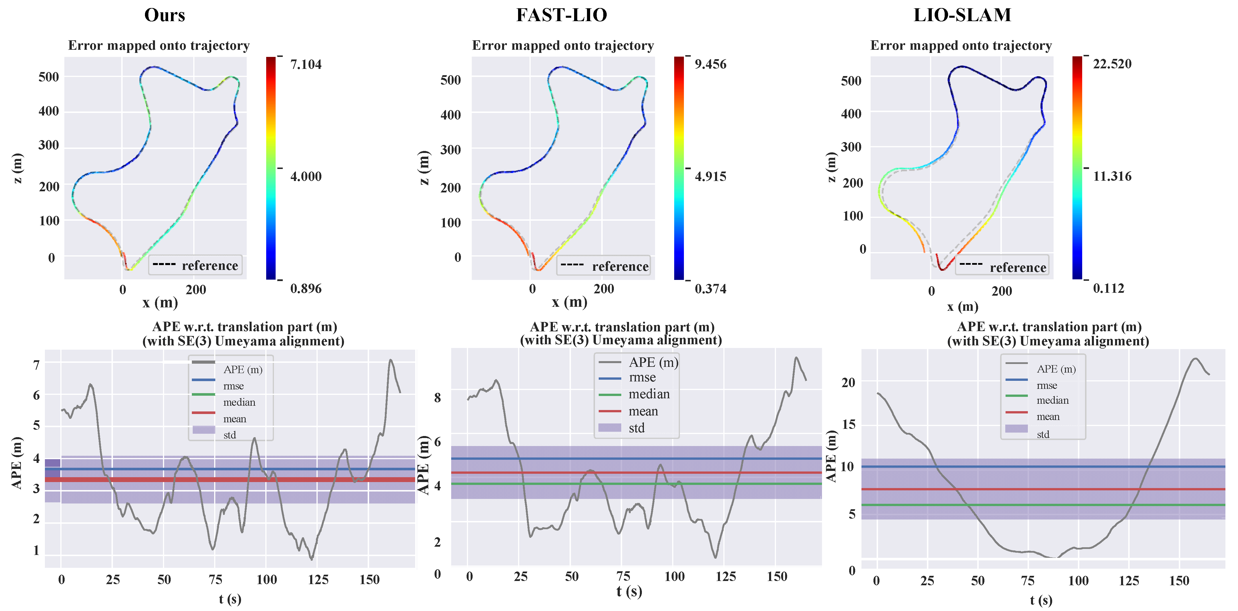
We conducted experiments on the publicly available KITTI dataset, specifically on sequences 0–10, using APE as the metric for evaluating the localization accuracy of our system. Additionally, we calculated the APE for LIO-SAM and FAST-LIO2, comparing their performance with our method. The results are shown in Figure 5.
As shown in Table 5 and Figure 5, the proposed algorithm demonstrates lower translation and rotation errors compared to FAST-LIO2, with a reduction in the root mean square error (RMSE) of translation error by approximately 3.8%. When compared to LIO-SAM, there is a more noticeable decrease in error metrics, making it less likely for significant errors to occur. The experimental results suggest that the proposed method is more suitable for use in terrestrial SLAM systems due to its relatively higher robustness and stability.

4.2.2. Loop Closure Experiment

The Loop Closure Experiment in SLAM is crucial in evaluating and enhancing the system’s accuracy and consistency. Through this experiment, we can test the system’s cumulative errors over extended operation and its robustness in dynamic environments.
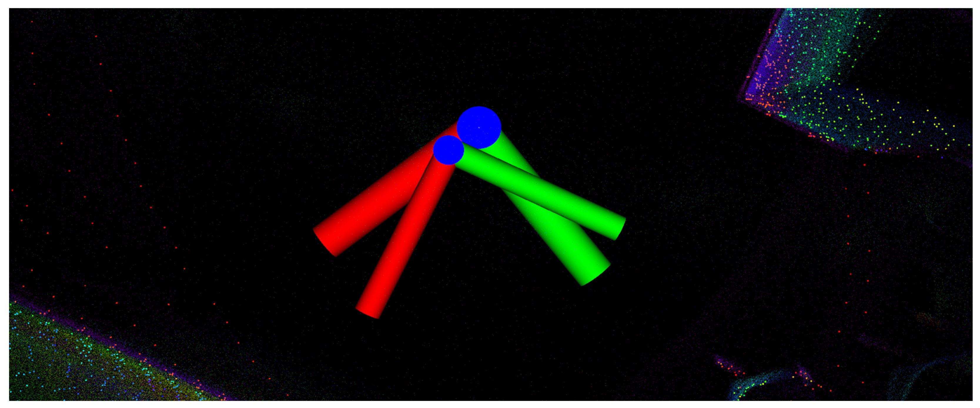
In our indoor state localization experiment, we conducted a loop closure test using the collected dataset to assess the stability of the SLAM system’s positioning. A robot was programmed to traverse a predetermined path of 340 m and return to the starting point. The initial and final positions estimated by the slam system were recorded to calculate the positioning error upon return, based on the distance between these two points, shown in Figure 6. To thoroughly assess the robot’s state estimation capabilities, three different motion strategies were employed along the set route:
  • Motion 1. Linear movement at 0.7 m/s across a flat surface, completing a circuit and returning to the start.
  • Motion 2. Zigzagging motion with the robot swaying left and right, moving in a curved path around the room at an average speed of approximately 0.7 m/s before returning to the starting point.
  • Motion 3. Straight-line movement over uneven terrain, completing a circuit and returning to the start, maintaining an average speed of 0.7 m/s.
Figure 7 illustrates the experimental setup. Each route featured numerous pedestrians walking randomly around the system and doors opening and closing randomly to alter the experimental environment. This setup was used to test the effectiveness of the system’s positioning technology under the uncertainty and dynamic conditions of real-world environments.
Each motion type was repeated three times to mitigate random errors, with the average results recorded in Table 6.
We also tested the FAST-LIO2 and LIO-SAM systems under the same dataset, with the results shown in Table 7. The experimental results indicated that the drift of this experiment is less than 0.07% (the maximum drift of 340 m is less than 0.22 m), which is nearly identical in accuracy to FAST-LIO2 and represents a significant improvement over LIO-SAM. On average, each scan identified 1421 valid feature points, enabling the SLAM system to accurately track the vehicle’s position and trajectory. Even with the presence of numerous dynamic obstacles during tests, the system showcased its capability for precise state localization within complex indoor environments. It retained high accuracy and robustness against diverse terrains and obstacles.

4.2.3. 3D Reconstruction Experiment

The most significant advantage of 3D LiDAR is its ability to provide high-precision three-dimensional spatial data, enabling this SLAM system to accomplish high-precision mapping and surveying tasks. To verify the capabilities of the LIO-FICP in this regard, we conducted indoor and outdoor ground vehicle experiments.
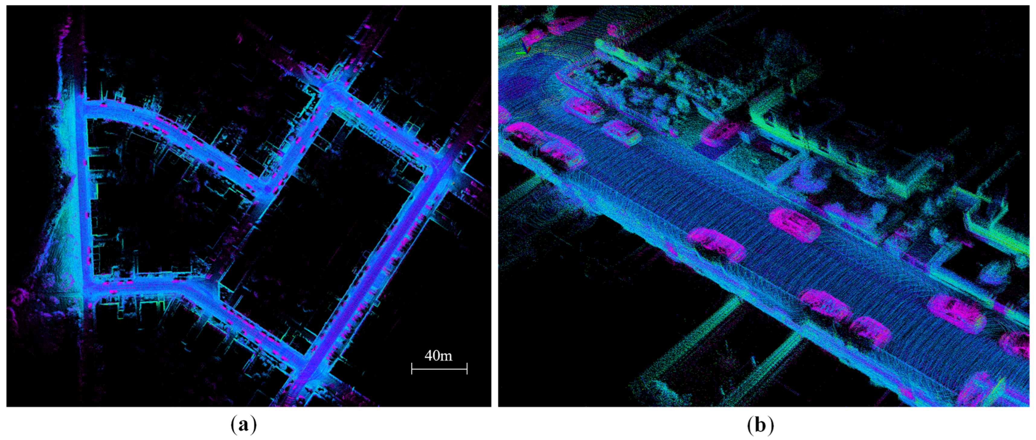
Outdoors, we ran our algorithm using the KITTI dataset to generate a reconstructed 3D road map, as shown in Figure 8. The map distinctly shows vehicles parked along the curb and permanent buildings, which is highly consistent with the scenes depicted in the RGB data from the dataset. During the experiment, the vehicle started from the origin and circled back to the starting point, completing a loop that is visible on the map, demonstrating the high accuracy of our mapping algorithm. Moreover, despite the presence of many moving vehicles and pedestrians along the route, dynamic objects were not represented in the mapping results, reflecting the precision and robustness of our algorithm.
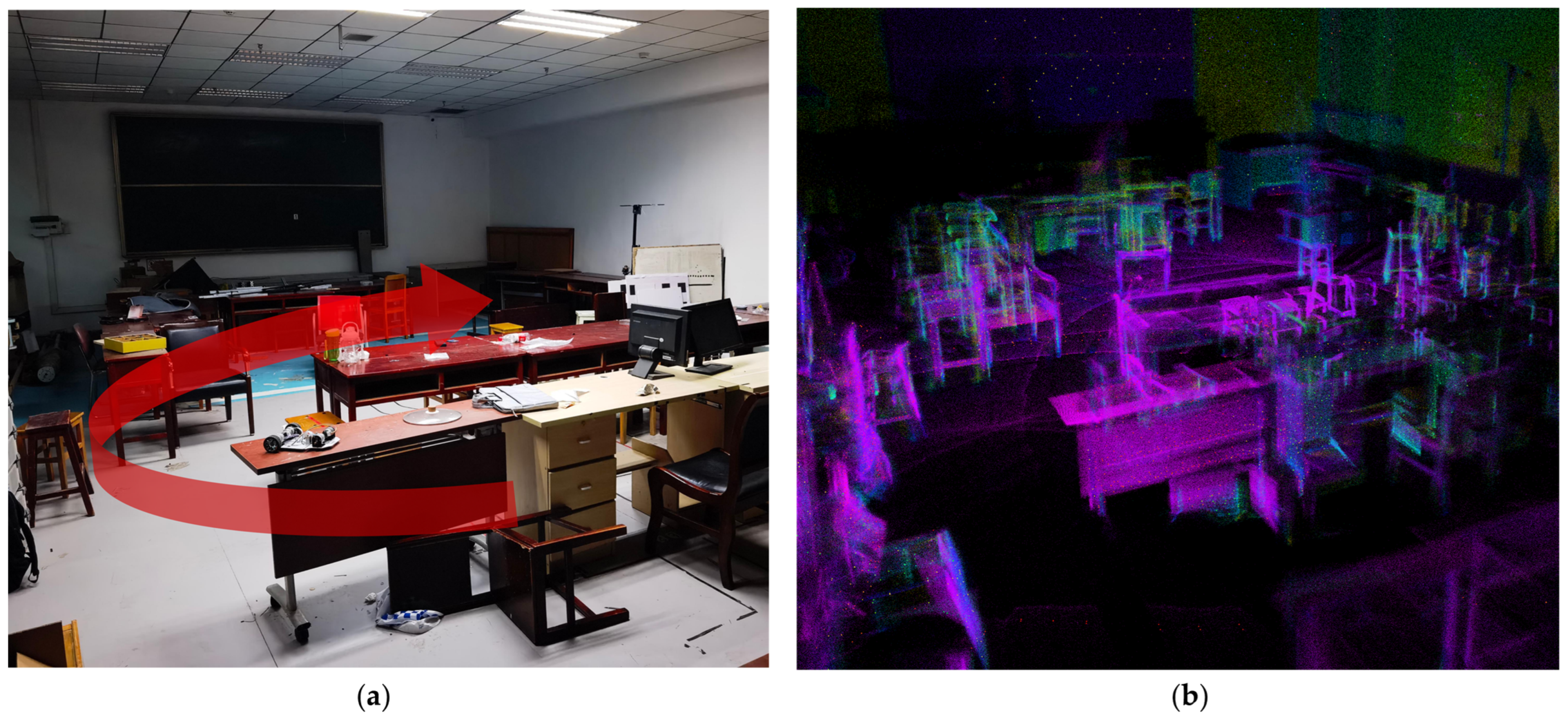
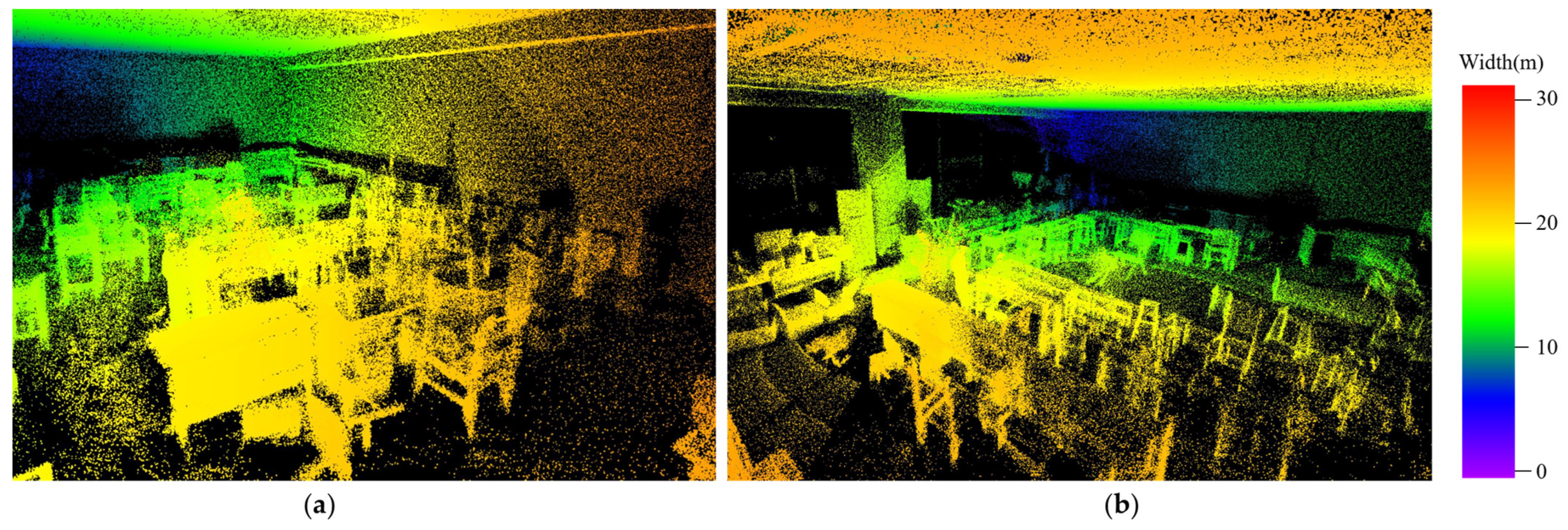
Based on a pre-constructed grid map, a route was manually planned within a 35 m × 15 m room; the arrow in Figure 9a. shows the general direction The robot circled the room before moving towards the center, reconstructing the indoor environment in the process. The room layout was a flat quadrilateral with a height of approximately 3.5 m, furnished with tables, chairs, and other irregular items, adding complexity to the mapping task. The vehicle was deliberately not directed to the room’s corners to evaluate the SLAM system’s comprehensive 3D reconstruction capability with limited path information. Utilizing the Fast-ICP algorithm, the LiDAR-Inertial Odometry allowed for the creation of a highly detailed room map, as shown in Figure 9b, capturing fine details like tables and chairs.
The system was then tested in a mixed indoor-outdoor environment. Compared to simple indoor rooms, this setting offers more extensive spaces with numerous dynamic elements, necessitating the system to process more data and exhibit greater robustness. Due to the increased size of the area, longer mapping durations might lead to IMU drift, potentially causing overlaps and distortions in the building structure.
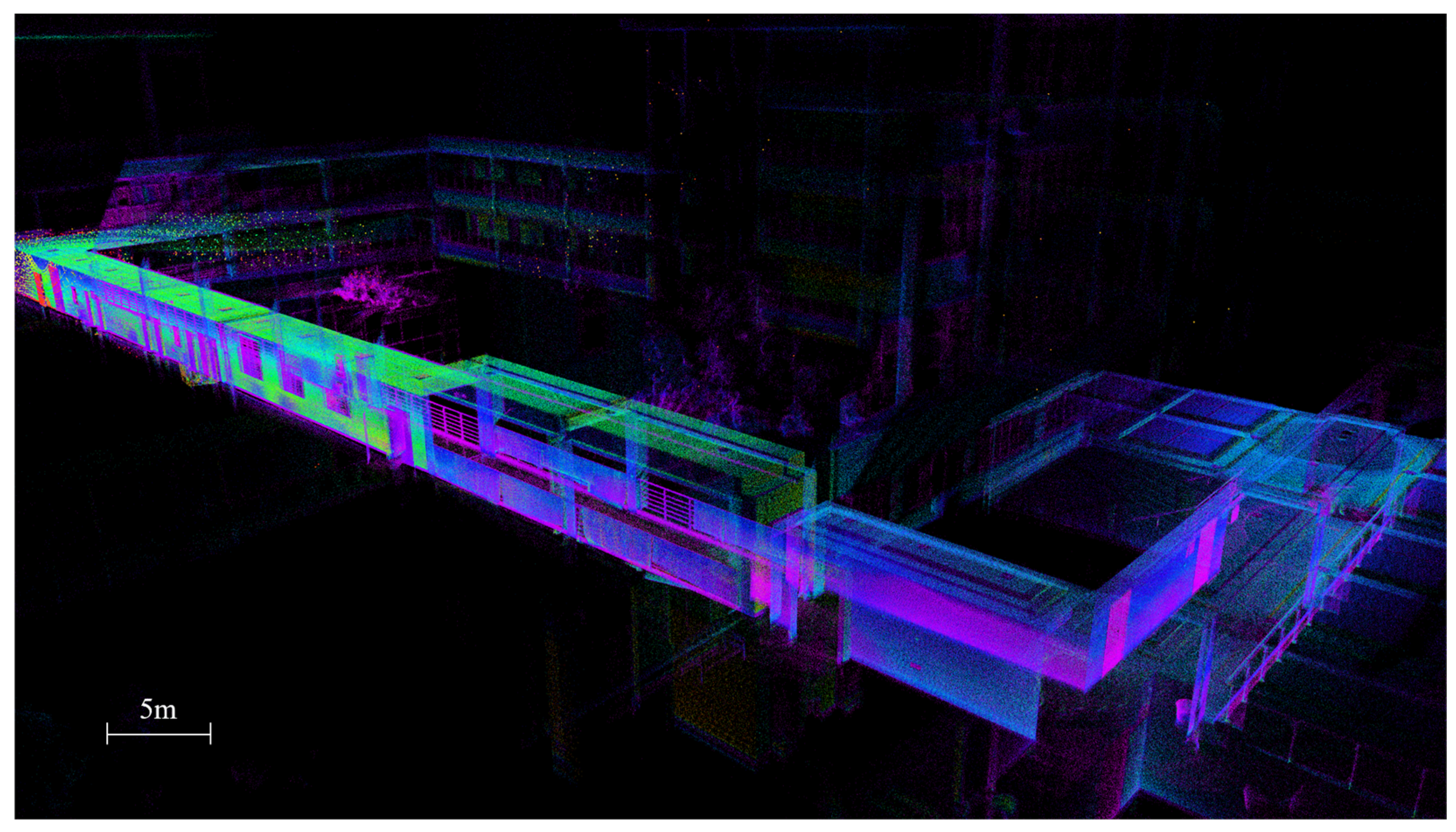
A start and end point were designated for the system, with the vehicle initiating its navigation task indoors before moving outdoors at about 0.7 m/s through the corridor to reach the predetermined endpoint. The corridor is surrounded by an open outdoor environment, significantly increasing the computational load. Figure 10 shows the actual test scenario, with the vehicle’s general direction of movement indicated by arrows.
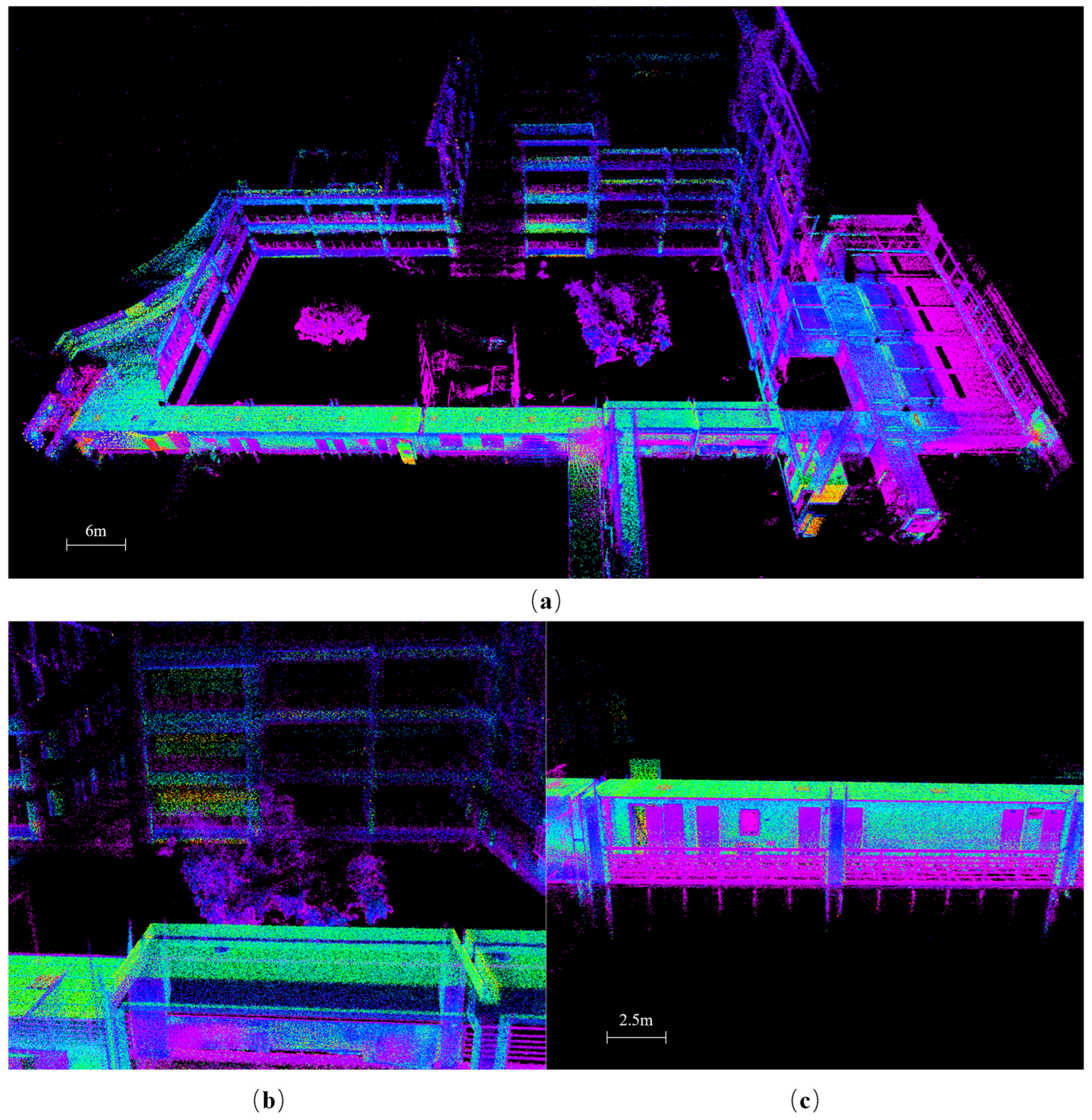
Figure 11 displays the system’s mapping results. The results show that LIO-FICP performs exceptionally well, successfully accomplishing 3D reconstruction of road sections and enabling the mapping and recognition of distant outdoor landscapes. The details of the outdoor parts, such as leaves and corridors, can be clearly seen in Figure 12.
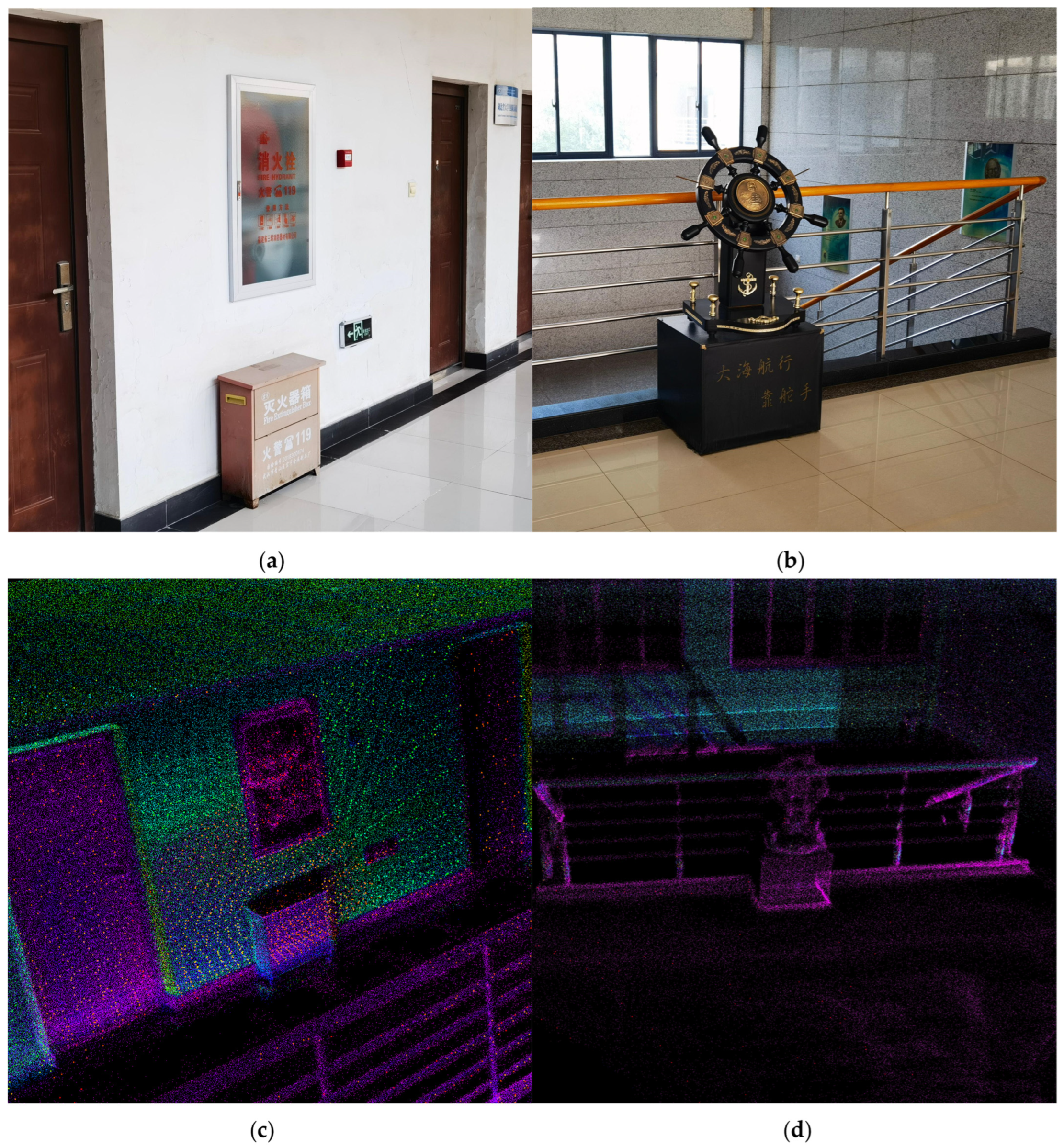
Figure 13 displays more detailed sections of the reconstructed map. Despite the brief period of point cloud accumulation, delicate structures like floor decorations and fire extinguisher cabinets are distinctly visible, demonstrating the SLAM system’s high-precision mapping capability and robustness.
The time taken by the vehicle from departure to the complete preservation of the 3D model was recorded and compared with the vehicle’s movement time. Our calculations show that the system ceased reconstruction immediately after the vehicle stopped and exported the model file within 5 s, confirming the real-time performance of the SLAM system.

4.3. Auto-Exploration Experiment

After completing the localization and mapping experiments with our SLAM system, we deployed it for RRT Exploration within the same system. We continued to test the autonomous exploration capabilities of the SLAM system indoors. The overall 3D Auto-Exploration Using RRT framework was implemented in ROS and C++, under the same configuration. To more comprehensively assess our system’s autonomous exploration abilities, we chose an indoor environment designed with a variety of obstacles, different terrains, and complex spatial layouts for experimentation.
We used the same indoor environment as in Section 4.2.3 to test it. At the start of the experiment, we manually placed the robot at the center of the map for initialization. After setting the boundaries of the map, the robot began its autonomous exploration. During the exploration process, the robot dynamically planned its path using the RRT algorithm to avoid obstacles and efficiently cover unknown areas. The 3D multi-goal RRT works as shown in Figure 14; the exploration path is generated on a 2D plane, although the car will eventually be reconstructed on a 3D map. We paid special attention to the robot’s responsiveness to sudden obstacles and its navigation and obstacle avoidance efficiency in complex environments. Multiple experiments ensured the system’s exploration was robust and continuous.
The experimental results demonstrated that our SLAM system, combined with the 3D RRT exploration framework, was capable of effectively carrying out autonomous exploration within complex indoor environments, while 2D RRT exploration always failed to explore this room. The robot was able to update the map information in real time and dynamically adjust its path based on newly discovered obstacles and unexplored areas. When encountering unknown obstacles, the robot was able to react quickly and re-plan its path, showing good obstacle avoidance capabilities.
The 2D RRT exploration fails to perceive the dimensions of obstacles, resulting in incorrect path planning in front of spatially featured obstacles, and thus fails to explore a complete map (grid map, not a 3D point cloud), as shown in Figure 15. Additionally, traditional RRT exploration lacks specific trajectory tracking optimization, leading to motion deadlocks in some narrow areas from which it cannot escape, culminating in the failure of RRT Exploration in room exploration.
Figure 16 illustrates the maps explored by the robot after the experiment, indicating that the robot covered most of the unknown areas and the path selection was highly optimized. The experimental results demonstrated that our SLAM system, combined with the RRT exploration framework, was capable of effectively carrying out autonomous exploration within complex indoor environments. The robot was able to update the map information in real time and dynamically adjust its path based on newly discovered obstacles and unexplored areas. When encountering unknown obstacles, the robot was able to react quickly and re-plan its path, showing good obstacle avoidance capabilities.

4.4. Analysis of the Resource Occupancy

SAR and VMstat are two commonly used system performance monitoring tools in sysstat (https://github.com/sysstat/sysstat (accessed on 20 January 2024)) widely used in operating systems to monitor system performance and resource usage.
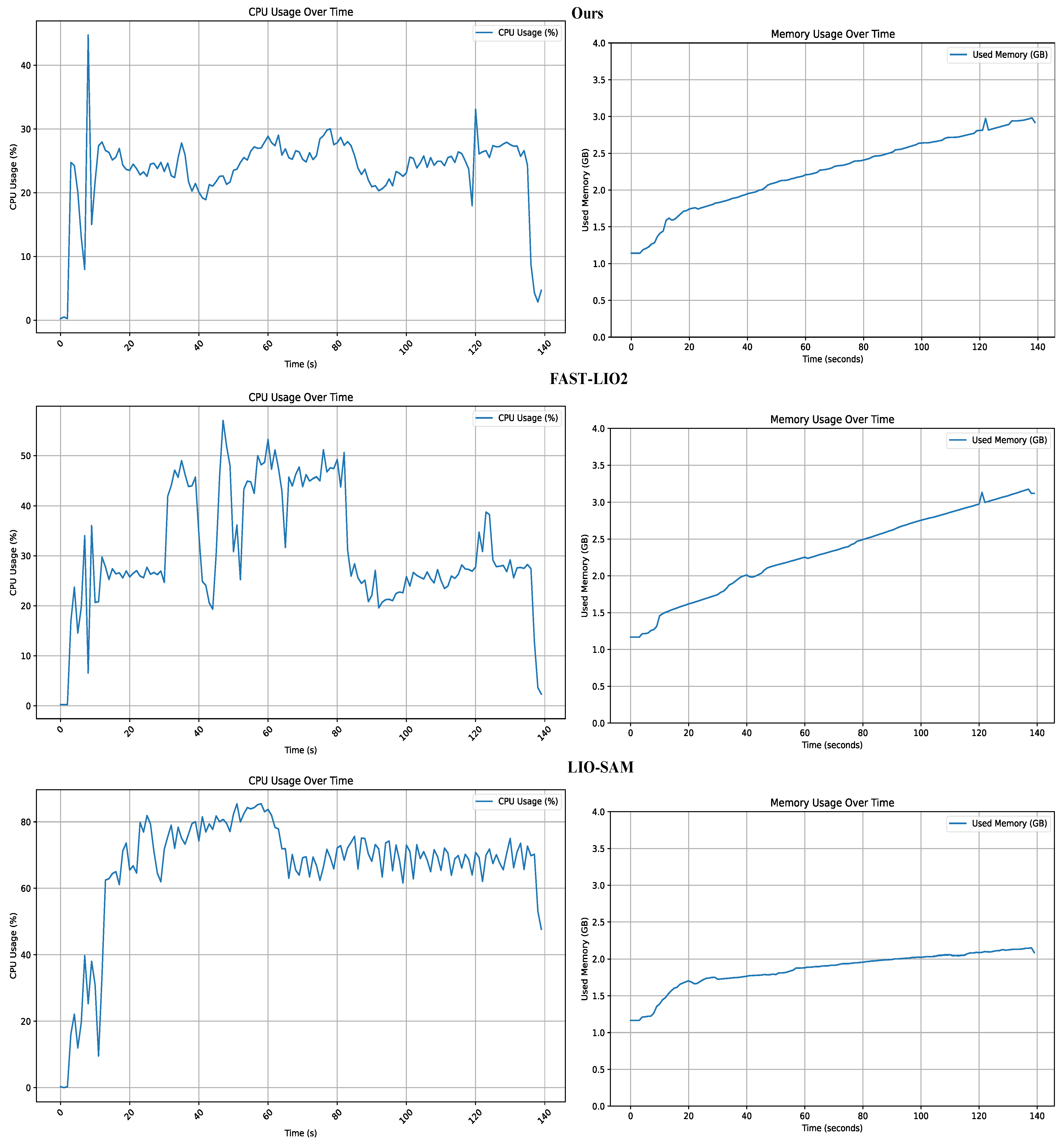
Since this SLAM system primarily utilizes CPU and memory resources, we employed the ‘SAR’ and ‘VMstat’ tools to monitor the CPU and memory usage in real time on our hardware platform, thus assessing the resource consumption of our algorithm. All tests were automatically conducted in a consistent environment using scripts and carried out on the 4.1 dataset. We also measured the resource utilization of SLAM systems based on fast-lio2 and lio-sam for comparison. The results are shown in Figure 17.
Data from Figure 17 and Table 8 demonstrate that our method, compared to FAST-LIO2, has lower CPU resource usage and memory consumption. Although our method consumes slightly more memory than LIO-SAM, it offers higher positioning accuracy, lower loop closure errors, improved stability and robustness, and a significant advantage in CPU utilization. This makes it particularly suitable for cost-conscious SLAM systems. Experiments show that in cost-sensitive application scenarios, our system can achieve efficient spatial localization and mapping with lower operational costs, not only meeting the performance requirements of low-cost SLAM systems but also providing significant advantages in sustainability and practicality, thus enabling a wide range of real-world applications.

5. Discussion

We have designed a SLAM system that integrates LiDAR-Inertial Odometry with RRT Exploration. It is characterized by its low-cost yet efficient pose estimation, mapping, and autonomous 3D space exploration. The design encompasses three modules. To achieve high performance within budget constraints, we developed a stable and adaptable vehicle structure utilizing a four-wheel configuration, incorporating cost-effective sensors. Subsequently, we developed the SLAM algorithm based on the LiDAR-Inertial Odometry framework. We achieved continuous, higher accuracy at a significantly lower computational load than traditional LOAM algorithms through precise optimization of point cloud matching and pose estimation with the Fast ICP algorithm. Finally, we adapted and enhanced the 3D RRT Exploration algorithm, equipping the system with advanced autonomous exploration functionalities. As UAVs advance in SLAM and three-dimensional reconstruction fields, this system has the potential to be applied in outdoor Unmanned Aircraft Systems (UAS) [56], offering prospective applications in data collection and mapping with small drones [57].
However, three limitations remain:
  • Although the LiDAR-Inertial Odometry framework enhances the efficiency and accuracy of pose estimation, it still heavily relies on the quality of data collected by sensors. Sensor performance degradation in harsh environments could directly affect the system’s precision in localization and mapping.
  • While the 3D RRT Exploration algorithm grants the system high-performance autonomous exploration capabilities, its computational complexity substantially escalates in environments with dynamic obstacles, potentially diminishing exploration efficiency and prolonging reaction times. Additionally, we must conduct more experiments to adjust the NMPC weight parameters to make the system’s motion control smoother and easier to port.
  • Generating 3D maps offline necessitates extra storage, and activating 3D autonomous exploration and Fast ICP optimization concurrently can result in elevated memory consumption.

6. Conclusions

This paper presents a low-cost SLAM system design that maintains high-performance SLAM algorithms under budget constraints. First, in terms of hardware, we designed a small vehicle with a three-layer structure and four rubber wheels, incorporating a control system that enhances the SLAM system’s stability, adaptability, and load capacity, drawing inspiration from current mobile robot technologies. Secondly, we developed a foundational SLAM solution based on the LiDAR-Inertial Odometry and Fast ICP algorithm and melded it with a 3D multi-objective RRT Exploration strategy grounded in NMPC, not only adapts mainstream SLAM algorithms but also makes localized improvements for enhanced performance. Then, we designed the experiments that confirm our system’s capability for accurate localization and mapping in intricate indoor settings, as well as autonomous reconstruction and surveying. Finally, we open-sourced our work to provide a low-cost SLAM solution with high performance. Although our approach strikes a good balance between cost and performance, it still encounters some constraints that must be addressed in future works focused on developing cost-effective SLAM systems.

Author Contributions

Conceptualization, X.H. and L.Z.; Data curation, X.H.; Formal analysis, C.P., L.Z. and X.H.; Funding acquisition, X.H.; Methodology, C.P.; Writing—original draft, C.P.; writing—review & editing, C.P., L.Z. and X.H. All authors have read and agreed to the published version of the manuscript.

Funding

This research was funded by National Key R&D Program of China (No.2023YFC3209105) and the Fundamental Research Funds for the Central Universities (2042024kf0035).

Data Availability Statement

Code and datasets have been made available at: https://github.com/pcl5/Low-cost-system (accessed on 13 March 2024).

Conflicts of Interest

The authors declare no conflict of interest.

References

  1. Smith, R.C.; Cheeseman, P. On the representation and estimation of spatial uncertainty. Int. J. Robot. Res. 1986, 5, 56–68. [Google Scholar] [CrossRef]
  2. Durrant-Whyte, H.; Bailey, T. Simultaneous localization and mapping: Part I. IEEE Robot. Autom. Mag. 2006, 13, 99–110. [Google Scholar] [CrossRef]
  3. Grigorescu, S.; Trasnea, B.; Cocias, T.; Macesanu, G. A survey of deep learning techniques for autonomous driving. J. Field Robot. 2020, 37, 362–386. [Google Scholar] [CrossRef]
  4. Takleh, T.T.O.; Bakar, N.A.; Rahman, S.A.; Hamzah, R.; Aziz, Z. A brief survey on SLAM methods in autonomous vehicle. Int. J. Eng. Technol. 2018, 7, 38–43. [Google Scholar] [CrossRef]
  5. Singandhupe, A.; La, H.M. A review of slam techniques and security in autonomous driving. In Proceedings of the 2019 Third IEEE International Conference on Robotic Computing (IRC), Naples, Italy, 25–27 February 2019; pp. 602–607. [Google Scholar]
  6. Polvi, J.; Taketomi, T.; Yamamoto, G.; Dey, A.; Sandor, C.; Kato, H. SlidAR: A 3D positioning method for SLAM-based handheld augmented reality. Comput. Graph. 2016, 55, 33–43. [Google Scholar] [CrossRef]
  7. Liu, H.; Zhang, G.; Bao, H. Robust keyframe-based monocular SLAM for augmented reality. In Proceedings of the 2016 IEEE International Symposium on Mixed and Augmented Reality (ISMAR), Merida, Mexico, 19–23 September 2016; pp. 1–10. [Google Scholar]
  8. Chen, C.-W.; Chen, W.-Z.; Peng, J.-W.; Cheng, B.-X.; Pan, T.-Y.; Kuo, H.-C.; Hu, M.-C. A real-time markerless augmented reality framework based on SLAM technique. In Proceedings of the 2017 14th International Symposium on Pervasive Systems, Algorithms and Networks & 2017 11th International Conference on Frontier of Computer Science and Technology & 2017 Third International Symposium of Creative Computing (ISPAN-FCST-ISCC), Exeter, UK, 21–23 June 2017; pp. 127–132. [Google Scholar]
  9. Dissanayake, M.G.; Newman, P.; Clark, S.; Durrant-Whyte, H.F.; Csorba, M. A solution to the simultaneous localization and map building (SLAM) problem. IEEE Trans. Robot. Autom. 2001, 17, 229–241. [Google Scholar] [CrossRef]
  10. Montemerlo, M.; Thrun, S.; Koller, D.; Wegbreit, B. FastSLAM: A factored solution to the simultaneous localization and mapping problem. In Proceedings of the Eighteenth National Conference on Artificial Intelligence, Edmonton, AB, Canada, 28 July 2002–1 August 2002; pp. 593–598. [Google Scholar]
  11. Thrun, S.; Burgard, W.; Fox, D. A real-time algorithm for mobile robot mapping with applications to multi-robot and 3D mapping. In Proceedings of the 2000 ICRA. Millennium Conference. IEEE International Conference on Robotics and Automation. Symposia Proceedings (Cat. No. 00CH37065), San Francisco, CA, USA, 24–28 April 2000; pp. 321–328. [Google Scholar]
  12. Davison, A.J.; Reid, I.D.; Molton, N.D.; Stasse, O. MonoSLAM: Real-time single camera SLAM. IEEE Trans. Pattern Anal. Mach. Intell. 2007, 29, 1052–1067. [Google Scholar] [CrossRef] [PubMed]
  13. Mur-Artal, R.; Montiel, J.M.M.; Tardos, J.D. ORB-SLAM: A versatile and accurate monocular SLAM system. IEEE Trans. Robot. 2015, 31, 1147–1163. [Google Scholar] [CrossRef]
  14. Engel, J.; Schöps, T.; Cremers, D. LSD-SLAM: Large-scale direct monocular SLAM. In Proceedings of the European Conference on Computer Vision, Zurich, Switzerland, 6–12 September 2014; pp. 834–849. [Google Scholar]
  15. Mur-Artal, R.; Tardós, J.D. Orb-slam2: An open-source slam system for monocular, stereo, and rgb-d cameras. IEEE Trans. Robot. 2017, 33, 1255–1262. [Google Scholar] [CrossRef]
  16. Campos, C.; Elvira, R.; Rodríguez, J.J.G.; Montiel, J.M.; Tardós, J.D. Orb-slam3: An accurate open-source library for visual, visual–inertial, and multimap slam. IEEE Trans. Robot. 2021, 37, 1874–1890. [Google Scholar] [CrossRef]
  17. Chen, W.; Shang, G.; Ji, A.; Zhou, C.; Wang, X.; Xu, C.; Li, Z.; Hu, K. An overview on visual slam: From tradition to semantic. Remote Sens. 2022, 14, 3010. [Google Scholar] [CrossRef]
  18. Wang, D.; Watkins, C.; Xie, H. MEMS mirrors for LiDAR: A review. Micromachines 2020, 11, 456. [Google Scholar] [CrossRef] [PubMed]
  19. Liu, Z.; Zhang, F.; Hong, X. Low-cost retina-like robotic lidars based on incommensurable scanning. IEEE ASME Trans. Mechatron. 2021, 27, 58–68. [Google Scholar] [CrossRef]
  20. Ye, H.; Chen, Y.; Liu, M. Tightly coupled 3d lidar inertial odometry and mapping. In Proceedings of the 2019 International Conference on Robotics and Automation (ICRA), Montreal, QC, Canada, 20–24 May 2019; pp. 3144–3150. [Google Scholar]
  21. Almadhoun, R.; Taha, T.; Seneviratne, L.; Dias, J.; Cai, G. A survey on inspecting structures using robotic systems. Int. J. Adv. Robot. Syst. 2016, 13, 1729881416663664. [Google Scholar] [CrossRef]
  22. Yamauchi, B. Frontier-based exploration using multiple robots. In Proceedings of the Second International Conference on Autonomous Agents, Minneapolis, MN, USA, 10–13 May 1998; pp. 47–53. [Google Scholar]
  23. Chickering, D.M. Optimal structure identification with greedy search. J. Mach. Learn. Res. 2002, 3, 507–554. [Google Scholar]
  24. Mostegel, C.; Wendel, A.; Bischof, H. Active monocular localization: Towards autonomous monocular exploration for multirotor mavs. In Proceedings of the 2014 IEEE International Conference on Robotics and Automation (ICRA), Hong Kong, China, 31 May–7 June 2014; pp. 3848–3855. [Google Scholar]
  25. Placed, J.A.; Castellanos, J.A. A deep reinforcement learning approach for active SLAM. Appl. Sci. 2020, 10, 8386. [Google Scholar] [CrossRef]
  26. LaValle, S.M. Rapidly-Exploring Random Trees: A New Tool for Path Planning; TR 98-11; Department of Computer Science, Iowa State University: Ames, IA, USA, 1998. [Google Scholar]
  27. Grisetti, G.; Stachniss, C.; Burgard, W. Improving grid-based slam with rao-blackwellized particle filters by adaptive proposals and selective resampling. In Proceedings of the 2005 IEEE International Conference on Robotics and Automation, Barcelona, Spain, 18–22 April 2005; pp. 2432–2437. [Google Scholar]
  28. Zhang, J.; Singh, S. LOAM: Lidar odometry and mapping in real-time. In Proceedings of the Robotics: Science and Systems, Berkeley, CA, USA, 12–16 July 2014; pp. 1–9. [Google Scholar]
  29. Shan, T.; Englot, B. Lego-loam: Lightweight and ground-optimized lidar odometry and mapping on variable terrain. In Proceedings of the 2018 IEEE/RSJ International Conference on Intelligent Robots and Systems (IROS), Madrid, Spain, 1–5 October 2018; pp. 4758–4765. [Google Scholar]
  30. Lin, J.; Zhang, F. Loam livox: A fast, robust, high-precision LiDAR odometry and mapping package for LiDARs of small FoV. In Proceedings of the 2020 IEEE International Conference on Robotics and Automation (ICRA), Paris, France, 31 May–31 August 2020; pp. 3126–3131. [Google Scholar]
  31. Xu, W.; Zhang, F. Fast-lio: A fast, robust lidar-inertial odometry package by tightly-coupled iterated kalman filter. IEEE Robot. Autom. Lett. 2021, 6, 3317–3324. [Google Scholar] [CrossRef]
  32. Hess, W.; Kohler, D.; Rapp, H.; Andor, D. Real-time loop closure in 2D LIDAR SLAM. In Proceedings of the 2016 IEEE International Conference on Robotics and Automation (ICRA), Stockholm, Sweden, 16–21 May 2016; pp. 1271–1278. [Google Scholar]
  33. Xu, W.; Cai, Y.; He, D.; Lin, J.; Zhang, F. Fast-lio2: Fast direct lidar-inertial odometry. IEEE Trans. Robot. 2022, 38, 2053–2073. [Google Scholar] [CrossRef]
  34. Shan, T.; Englot, B.; Meyers, D.; Wang, W.; Ratti, C.; Rus, D. Lio-sam: Tightly-coupled lidar inertial odometry via smoothing and mapping. In Proceedings of the 2020 IEEE/RSJ International Conference on Intelligent Robots and Systems (IROS), Las Vegas, NV, USA, 24 October 2020–24 January 2021; pp. 5135–5142. [Google Scholar]
  35. Qin, C.; Ye, H.; Pranata, C.E.; Han, J.; Zhang, S.; Liu, M. Lins: A lidar-inertial state estimator for robust and efficient navigation. In Proceedings of the 2020 IEEE International Conference on Robotics and Automation (ICRA), Paris, France, 31 May–31 August 2020; pp. 8899–8906. [Google Scholar]
  36. Besl, P.J.; McKay, N.D. Method for registration of 3-D shapes. In Proceedings of the Sensor Fusion IV: Control Paradigms and Data Structures, Boston, MA, USA, 12–15 November 1991; pp. 586–606. [Google Scholar]
  37. Rusinkiewicz, S.; Levoy, M. Efficient variants of the ICP algorithm. In Proceedings of the Proceedings Third International Conference on 3-D Digital Imaging and Modeling, Quebec City, QC, Canada, 28 May–1 June 2001; pp. 145–152. [Google Scholar]
  38. Pomerleau, F.; Colas, F.; Siegwart, R. A review of point cloud registration algorithms for mobile robotics. Found. Trends Robot. 2015, 4, 1–104. [Google Scholar] [CrossRef]
  39. Clotet, E.; Palacín, J. Slamicp library: Accelerating obstacle detection in mobile robot navigation via outlier monitoring following icp localization. Sensors 2023, 23, 6841. [Google Scholar] [CrossRef]
  40. Grisetti, G.; Kümmerle, R.; Stachniss, C.; Burgard, W. A tutorial on graph-based SLAM. IEEE Intell. Transp. Syst. Mag. 2010, 2, 31–43. [Google Scholar] [CrossRef]
  41. Ristic, B.; Palmer, J.L. Autonomous exploration and mapping with RFS occupancy-grid SLAM. Entropy 2018, 20, 456. [Google Scholar] [CrossRef] [PubMed]
  42. Bundy, A.; Wallen, L. Breadth-first search. In Catalogue of Artificial Intelligence Tools; Springer: Berlin/Heidelberg, Germany, 1984; p. 13. [Google Scholar]
  43. Umari, H.; Mukhopadhyay, S. Autonomous robotic exploration based on multiple rapidly-exploring randomized trees. In Proceedings of the 2017 IEEE/RSJ International Conference on Intelligent Robots and Systems (IROS), Vancouver, BC, Canada, 24–28 September 2017; pp. 1396–1402. [Google Scholar]
  44. Mukhopadhyay, S.; Umari, H.; Koirala, K. Multi-robot Map Exploration Based on Multiple Rapidly-Exploring Randomized Trees. SN Comput. Sci. 2023, 5, 31. [Google Scholar] [CrossRef]
  45. Wu, Z.; Meng, Z.; Zhao, W.; Wu, Z. Fast-RRT: A RRT-based optimal path finding method. Appl. Sci. 2021, 11, 11777. [Google Scholar] [CrossRef]
  46. Kuffner, J.J.; LaValle, S.M. RRT-connect: An efficient approach to single-query path planning. In Proceedings of the 2000 ICRA. Millennium Conference. IEEE International Conference on Robotics and Automation. Symposia Proceedings (Cat. No. 00CH37065), San Francisco, CA, USA, 24–28 April 2000; pp. 995–1001. [Google Scholar]
  47. Cao, C.; Zhu, H.; Choset, H.; Zhang, J. TARE: A Hierarchical Framework for Efficiently Exploring Complex 3D Environments. In Proceedings of the Robotics: Science and Systems, Virtually, 12–16 July 2021; p. 2. [Google Scholar]
  48. Huston, J.C.; Graves, B.J.; Johnson, D.B. Three wheeled vehicle dynamics. SAE Trans. 1982, 91, 591–604. [Google Scholar]
  49. Gfrerrer, A. Geometry and kinematics of the Mecanum wheel. Comput. Aided Geom. Des. 2008, 25, 784–791. [Google Scholar] [CrossRef]
  50. Raitoharju, M.; Piché, R. On computational complexity reduction methods for Kalman filter extensions. IEEE Aerosp. Electron. Syst. Mag. 2019, 34, 2–19. [Google Scholar] [CrossRef]
  51. Bentley, J.L. Multidimensional binary search trees used for associative searching. Commun. ACM 1975, 18, 509–517. [Google Scholar] [CrossRef]
  52. Mayne, D.Q.; Rawlings, J.B.; Rao, C.V.; Scokaert, P.O. Constrained model predictive control: Stability and optimality. Automatica 2000, 36, 789–814. [Google Scholar] [CrossRef]
  53. Lindqvist, B.; Agha-Mohammadi, A.-A.; Nikolakopoulos, G. Exploration-RRT: A multi-objective path planning and exploration framework for unknown and unstructured environments. In Proceedings of the 2021 IEEE/RSJ International Conference on Intelligent Robots and Systems (IROS), Prague, Czech Republic, 27 September–1 October 2021; pp. 3429–3435. [Google Scholar]
  54. Ma, L.; Xue, J.; Kawabata, K.; Zhu, J.; Ma, C.; Zheng, N. Efficient sampling-based motion planning for on-road autonomous driving. IEEE Trans. Intell. Transp. Syst. 2015, 16, 1961–1976. [Google Scholar] [CrossRef]
  55. Rusu, R.B.; Cousins, S. 3d is here: Point cloud library (pcl). In Proceedings of the 2011 IEEE International Conference on Robotics and Automation, Shanghai, China, 9–13 May 2011; pp. 1–4. [Google Scholar]
  56. Zhang, S.; Bogus, S.M.; Lippitt, C.D.; Kamat, V.; Lee, S. Implementing remote-sensing methodologies for construction research: An unoccupied airborne system perspective. J. Constr. Eng. Manag. 2022, 148, 03122005. [Google Scholar] [CrossRef]
  57. Lippitt, C.D.; Zhang, S. The impact of small unmanned airborne platforms on passive optical remote sensing: A conceptual perspective. Int. J. Remote Sens. 2018, 39, 4852–4868. [Google Scholar] [CrossRef]
Figure 1. Pipelines of the traditional SLAM method.
Remotesensing 16 01979 g001
Figure 2. The results of the hardware design for the system, where (a) shows the vertical structure diagram of the cart, annotating the structure and items placed on each layer, and (b) depicts an actual photo of the system.
Remotesensing 16 01979 g002
Figure 3. An illustrative representation of the Fast-ICP enhanced LiDAR-inertial odometry structure.
Remotesensing 16 01979 g003
Figure 4. The 3D multi-goal RRT framework using the NMPC Trajectory Optimizer.
Remotesensing 16 01979 g004
Figure 5. APE of our method in the KITTI dataset: Sequence 9, FAST-LIO, and LIO-SAM.
Remotesensing 16 01979 g005
Figure 6. The vehicle’s starting point (coordinate system with thicker axis) and ending point (coordinate system with thinner axis) have been marked in Figure 6. The red, blue, and green axes represent the X, Y, and Z axes, respectively. We obtain the Drift Distance by comparing the positions of the two coordinate systems in time and space.
Remotesensing 16 01979 g006
Figure 7. Schematic diagrams of the car for the closed-loop test experiment. In the figure, the yellow line represents the planned scanning route, (a) is motion 1, (b) motion 2, (c) motion 3, and the red curve represents uneven terrain or dynamic obstacles.
Remotesensing 16 01979 g007
Figure 8. These are the mapping results of the outdoor environment. (a) The global map of the environment; (b) stationary vehicles on both sides of the road.
Remotesensing 16 01979 g008
Figure 9. These are figures of the indoor environment, the arrow direction represents the planned path direction. (a) The real scene of the test room; (b) the 3D reconstruction of the room.
Remotesensing 16 01979 g009
Figure 10. Indoor-outdoor environment: the system starts indoors and passes through a corridor surrounded by outdoors to reach the destination. The arrow direction represents the planned path direction.
Remotesensing 16 01979 g010
Figure 11. The mapping result of indoor-outdoor environment, the system starts indoors and passes through a corridor surrounded by outdoors to reach the destination.
Remotesensing 16 01979 g011
Figure 12. These are figures of the Indoor-outdoor environment. (a) The top-down point cloud map of the entire environment; (b) shows the details of tree reconstruction, with visible branches and leaves; (c) shows the reconstruction results of the corridor.
Remotesensing 16 01979 g012
Figure 13. The reconstruction effect of the detail part. (a,c) Physical drawings and point clouds of fire extinguisher hydrants. (b,d) Physical drawings and point clouds of decorations.
Remotesensing 16 01979 g013
Figure 14. This is the process of multi-goal RRT growth. The parameter for cell size in the grid is 1, meaning that each grid cell represents a 1 m × 1 m area.
Remotesensing 16 01979 g014
Figure 15. The illustration shows incorrect path planning by 2D RRT Exploration. We converted three-dimensional LiDAR point clouds into two-dimensional point clouds through filtering, which fails to detect obstacles above the space. This leads to erroneous path planning and can result in collisions or even overturning of the robot.
Remotesensing 16 01979 g015
Figure 16. This is the result of the 3D multi-goal RRT exploration. (a,b) The reconstruction from different angles of the room.
Remotesensing 16 01979 g016
Figure 17. This is the results of system resource occupancy testing, conducted simultaneously with the experiments described in Section 4.2.3.
Remotesensing 16 01979 g017
Table 1. Relevant information about the MID-360 LiDAR scanner used in our system.
SpecificationDescription
Laser Wavelength905 nm
Detection Range (@ 100 klx)40 m @ 10% reflectivity
70 m @ 80% reflectivity
Close Proximity Blind Zone 20.1 m
Point Rate200,000 points/s (first return)
Frame Rate10 Hz (typical)
IMUICM40609
FOVHorizontal: 360°
Vertical: −7°~52°
Range Precision 3 (1σ)≤2 cm 4 (@ 10 m)
≤3 cm 5 (@ 0.2 m)
Angular Precision (1σ)<0.15°
2 Target objects within 0.1 to 0.2 m from Mid-360 can be detected and point cloud data can be recorded. However, since the detection precision cannot be guaranteed, the data should be taken as a reference only. 3 To detect objects having different reflectivities within the detection range, the accuracy of point cloud data of very few positions might decrease slightly. 4 Tested in an environment at a temperature of 25 °C (77 °F) with a target object that has a reflectivity of 80% and is 10 m away from Livox Mid-360. 5 Tested in an environment at a temperature of 25 °C (77 °F) with a target object that has a reflectivity of 80% and is 0.2 m away from Livox Mid-360. For target objects within 0.1 to 1 m away from the Mid-360, if they have a low reflectivity or are thin and tiny, the detection effect cannot be guaranteed. These objects include but are not limited to black foam and the surface of water or objects that have been polished, have a matte finish, thin lines, etc.
Table 2. Cost breakdown of SLAM system components.
ComponentDescriptionQuantityUnit Cost ($)Total Cost ($)
Mid-3603D LiDAR sensor with IMU1749556.44
Jetson nano 4 GBSoC, Data Processing Unit1129129
STM32F407VET6MCU, ROS base plate master control223.547
carbon plate-ABody structure, porous rectangles12020
carbon plate-BLiDAR Support Structure155
MG513 motorDC-coded motor, with rubber wheel46.9727.89
Battery4000 mAh-30C and 1200 mAh-45C 45
OthersAll kinds of wire and copper column 10
Total Cost 840.33
Table 3. Comparison of SLAM robot models by cost and capabilities.
ModelRobot TypeLiDAR SLAM DimensionSoC/CPUAuto ExplorationCost ($)
Turtlebot4Two-wheeled mobile robot2D LiDARRaspberry Pi 4BNo2191.44
Hiwonder JetAuto ProOmnidirectional mobile robot2D LiDARJetson nano2D1399.99
SLAMTEC HermesMobile robot with 2-wheel hub motor2D LiDARUnknownNo3061.17
Unitree Go 2Robot dog3D LiDAR8 core CPUUnknown2588.08
WEILAN AlphaDog C 2022Robot dog3D LiDARARM 64 bitUnknown5134.41
OursFour-wheeled mobile robot3D LiDARJetson nano3D840.33
Table 4. Experimental Environment.
NameVersion
OSUbuntu 18.04
SoCNVIDIA Tegra X1
RAM4 GB
ROM64 GB
Accelerator LibraryPCL v1.9.1 + Eigen v3.3.4
Table 5. Comparative results of localization errors in the KITTI.
APETranslation Error (m)Rotation Error (Degrees)
Algorithm MaxMeanMinRMSEMaxMeanMinRMSE
Ours7.1042.5410.1922.8722.4792.4342.3462.435
FAST-LIO29.4562.6430.2042.9862.5022.4402.3462.440
LIO-SAM51.8924.8310.1128.3232.8282.3151.4812.361
Table 6. Our method’s drift results of the loop closure test experiment.
Motion StrategiesDrift (m)
XYZ
Linear + Flat0.0169420.0034760.157648
Zigzagging + Flat0.0162890.0046510.173591
Linear + Uneven0.0160750.0089720.210820
Table 7. The results of the maximum drift loop closure experiment.
AlgorithmMax Drift (m)Accuracy
XYZ
LIO-SAM (LoopClosutre Disable)1.2266390.2959071.3646430.54676%
FAST-LIO20.0321260.0167370.2785910.10450%
Ours0.0160750.0089720.2108200.06235%
Table 8. The average CPU and memory usage results of the SLAM system during testing.
AlgorithmThe Average CPU UsageThe Average Memory Usage
LIO-SAM66.75%47.54%
FAST-LIO230.32%56.73%
Ours23.66%52.45%
Disclaimer/Publisher’s Note: The statements, opinions and data contained in all publications are solely those of the individual author(s) and contributor(s) and not of MDPI and/or the editor(s). MDPI and/or the editor(s) disclaim responsibility for any injury to people or property resulting from any ideas, methods, instructions or products referred to in the content.