Article

ESatSR: Enhancing Super-Resolution for Satellite Remote Sensing Images with State Space Model and Spatial Context

1
School of Information Science and Technology, ShanghaiTech University, Shanghai 201210, China
2
Innovation Academy for Microsatellites, Chinese Academy of Sciences, Shanghai 201210, China
3
College of Biomedical Engineering, Sichuan University, Chengdu 610065, China
4
School of Optoelectronics, University of Chinese Academy of Sciences, Beijing 100094, China
*
Author to whom correspondence should be addressed.
These authors contributed equally to this work.
Remote Sens. 2024, 16(11), 1956; https://doi.org/10.3390/rs16111956
Submission received: 30 March 2024 / Revised: 17 May 2024 / Accepted: 29 May 2024 / Published: 29 May 2024
(This article belongs to the Special Issue Deep Learning for Remote Sensing Image Enhancement)

Abstract

:
Super-resolution (SR) for satellite remote sensing images has been recognized as crucial and has found widespread applications across various scenarios. Previous SR methods were usually built upon Convolutional Neural Networks and Transformers, which suffer from either limited receptive fields or a lack of prior assumptions. To address these issues, we propose ESatSR, a novel SR method based on state space models. We utilize the 2D Selective Scan to obtain an enhanced capability in modeling long-range dependencies, which contributes to a wide receptive field. A Spatial Context Interaction Module (SCIM) and an Enhanced Image Reconstruction Module (EIRM) are introduced to combine image-related prior knowledge into our model, therefore guiding the process of feature extraction and reconstruction. Tailored for remote sensing images, the interaction of multi-scale spatial context and image features is leveraged to enhance the network’s capability in capturing features of small targets. Comprehensive experiments show that ESatSR demonstrates state-of-the-art performance on both OLI2MSI and RSSCN7 datasets, with the highest PSNRs of 42.11 dB and 31.42 dB, respectively. Extensive ablation studies illustrate the effectiveness of our module design.

Graphical Abstract

1. Introduction

Remote sensing is an important ground observation technology that has rapidly developed in recent years. Due to its wide coverage and high accessibility, it has been widely used in disaster detection, early warning, resource exploration, land cover classification, and other fields. High-resolution satellite remote sensing images are widely applied across various scenarios such as change detection [1,2] and object detection [3,4]. Due to the far distance between spacecrafts and the ground, satellite remote sensing images span extensive geographic areas, but the spatial resolution is relatively low, resulting in numerous small targets appearing in the images. Furthermore, the quality of images captured by satellite sensors is constrained by the space imaging equipment and communication bandwidth. Moreover, various factors affect the image quality in practical use, such as electronic noise, optical aberrations, atmospheric blurring, and motion blur [5]. Although these issues can be addressed by improving the satellite and the camera, it significantly increases development costs. Due to these factors, the analysis and comprehension of remote sensing images are challenging and complicated. Therefore, finding ways to enhance image quality without introducing more cost is a significant task in the field of remote sensing.
In recent years, with the significant development of deep learning technology, super-resolution (SR) methods have been introduced and applied to enhance remote sensing images. In the application of satellite remote sensing images, image registration [6,7] and SR [8,9] are two crucial pre-processing steps for downstream tasks. SR has always been one of the hot tasks in the field of computer vision, aiming to restore images from low-resolution (LR) images to become high-resolution (HR) images. Since the groundbreaking work of SRCNN [8] that first used the Convolutional Neural Network (CNN) in the SR field, CNN has become the most popular universal framework for SR tasks [10,11]. Many excellent SR methods based on CNN have sophisticated structural designs, and due to the utilization of convolution, CNNs usually have good local information extraction capabilities, demonstrating competitive performance. At the same time, as an alternative to CNN, the Vision Transformer (ViT) [12] has shown remarkable performance in addressing challenging tasks in the field of computer vision. Its self-attention mechanism effectively captures the intrinsic relationships among global visual content. ViT has achieved state-of-the-art results in classic computer vision tasks such as image classification [12] and object detection [13], while also demonstrating dominance in the SR field [14,15].
Despite the success that CNNs and ViTs have achieved, these two paradigms still suffer from several limitations. In terms of CNNs, firstly, the convolution kernel is content-irrelevant to the specific content of images. Reconstructing different regions with the same convolution kernel leads to insufficient generalization ability. Secondly, the receptive field of the convolutional layer is strictly limited by the size of the convolution kernel, which means the convolutional layer merely focuses on local information and the result usually contains strong local biases, which is not effective for situations requiring long-distance modeling [16]. As for ViTs, vanilla transformers, known as the plain ViT, are pre-trained on massive huge multi-modal datasets, including images, videos, and texts, which allows the model to learn powerful representations that can effectively extract image features. However, the plain ViT’s reliance on pre-training prevents it from structural modifications which contain prior assumptions of vision tasks. Consequently, due to its lack of vision specific knowledge, the plain ViT achieves sub-optimal performance when applied to vision tasks [17,18]. While SwinIR [16] attempts to introduce more vision-related prior information through utilizing the shifted window mechanism, this strategy inadvertently compromises the Transformer architecture’s inherent capability to model long-range dependencies, resulting in a limited receptive field [19], as shown in Figure 1.
To address these limitations, we propose ESatSR, an SR model specifically designed for remote sensing images based on state space models (SSMs). We apply 2D Selective Scan (SS2D) [21] to ensure the model possesses the capability of modeling long-range dependencies, which contributes to a wide receptive field. Spatial context is introduced to supplement visual prior assumptions, while its multi-scale design tailors the network’s capability to effectively capture features of small objects, aligning with the characteristic of remote sensing images. Our ESatSR consists of three parts: the Feature Extraction module, Spatial Context Interaction Module, and Enhanced Image Reconstruction Module. The feature extraction module includes a shallow feature extractor and a deep feature extractor. The shallow feature extractor converts the LR image from the image dimension to the feature dimension, with low-frequency information of the image still preserved. The deep feature extractor utilizes SS2D to obtain high-frequency features with global attention. We designed the Spatial Context Interaction Module to bring spatial priors to the network, thereby supplementing it with multi-scale, fine-grained information for super-resolution. The Enhanced Image Reconstruction Module combines shallow features, deep features, and spatial context simultaneously to produce high-quality SR images.
The major contributions in this work are summarized as follows:
  • We propose ESatSR, an SR model designed for remote sensing images based on state space models. It can effectively conduct super-resolution in satellite remote sensing image scenarios, and our experiments demonstrate that ESatSR outperforms several state-of-the-art methods, including CNNs as well as Transformers, on public remote sensing datasets.
  • We design a module utilizing the state space model (SSM) as a solution to enhancing long-range dependencies, named RVMB. Benefiting from the SSM’s wide receptive field, RVMBs exhibit powerful long-range modeling capabilities compared to modules based on CNNs or Transformers, and perform well in both global and local feature extraction tasks, thereby enhancing the model’s overall performance.
  • We propose the Spatial Context Interaction Module to address the lack of prior assumptions. By introducing spatial prior information, ESatSR can utilize image prior knowledge to guide the image feature extraction process, and the interaction between multi-scale spatial context and image features enhance the network’s capability in capturing small targets, thereby leading to enhanced model performance on remote sensing images.

2. Related Work

2.1. Image Restoration

Image restoration aims to recover an image from its degraded version. Methods of image restoration can be used for dehazing, deblurring, super-resolution, etc. The SRCNN [8] was the first work to introduce convolutional neural networks into the realm of image restoration and achieve superior results compared to traditional methods. Since then, CNN-based methods have gradually become the mainstream framework in image restoration domain. Many works based on CNN [10,11,22,23,24] have been proposed to further enhance the quality of image restoration. Some of these works have incorporated sophisticated designs in networks, such as residual connections [20,25] and dense connections [26]. Several works [20] developed attention mechanisms within CNN structures to allow models to more effectively utilize pixel information. Ref. [24] combined non-local self-attention with sparse representation, proposing a sparse global attention module that reduces the computational load of the model. Despite the improvements made to CNN in the aforementioned works, the irrelevance between convolutional kernels and image content has not been effectively addressed. Therefore, more researchers have explored different network structures for image restoration, such as recursive neural networks (RNNs) [27], graph neural networks (GNNs) [28], and generative adversarial networks (GANs). GAN is also one of the mainstream frameworks in computer vision. It works by setting up two networks (usually a generator and a discriminator) with opposite goals and training them adversarially. For instance, the generator aims to generate fake images similar to real images, while the discriminator aims to distinguish whether the input image is real or fake. Many works have developed image restoration methods based on GAN, such as SRGAN [9], ESRGAN [29], and Real-ESRGAN [30]. SRGAN and ESRGAN introduce perceptual loss during training to enhance the visual quality of output images. Real-ESRGAN employs a downsample network to learn the image degradation in real world, aiming to generate synthetic LR images which is more suitable for model training. However, despite its advantages, GAN still suffers from issues like unstable training, difficulty in convergence, and the potential for generators to take shortcuts, which means it directly outputs the original image.
In recent years, the Transformer has become increasingly popular in computer vision and has taken a dominant position in most computer vision tasks. The original Transformer was initially designed for NLP. With ViT [12] introducing an almost unmodified Transformer into image classification for the first time, there has been a growing number of Transformer-based works in the field of computer vision. Due to its ability to learn the relationships between different blocks in an image, it can focus on regions that are more important for the results, and this mechanism is usually called attention. The attention mechanism enables the Transformer to outperform CNNs, achieving impressive results in areas such as object detection [13,31] and image segmentation [32,33,34]. Inspired by the success of the Transformer in other fields, IPT [14], a universal framework based on the Transformer for various image restoration tasks, was proposed. VSR-Transformer [15] combines CNN with a Transformer for better feature extraction. SwinIR [16], an SR method based on Swin Transformer [35], introduces the attention mechanism with shifted window, allowing the model to have the advantages of both CNNs and Transformers, that is, strong local feature extraction capability and attention mechanism, thereby producing state-of-the-art results on multiple datasets.

2.2. Image Super-Resolution for Remote Sensing

Due to the unique value demonstrated by high-quality remote sensing images in multiple application areas, research on super-resolution for remote sensing images has gradually attracted more attention. The spatial resolution of remote sensing images is crucial for downstream tasks. The higher the resolution of the image, the more accurate the results of downstream tasks such as target detection, change detection, and target tracking. However, without adding new meaningful information, simply upsampling the image through interpolation will not lead to better results for downstream tasks. Therefore, a number of learning-based super-resolution methods have been proposed in the field of remote sensing, aiming to extract hidden information in pixels to restore high-resolution remote sensing images.
Different from natural images, due to the far distance between the aircraft and the ground, remote sensing images cover a wider area and have lower spatial resolution, and consequently, there are dozens of small targets occurring in remote sensing images, which poses a challenge for super-resolution. Effectively handling these dense and small targets that occupy only a few pixels is crucial for achieving higher performance in the super-resolution for remote sensing images. LGCNet [36] was the first to introduce the SR method into the realm of remote sensing image. Based on a traditional CNN architecture, it can effectively extract image features both locally and globally. In [37], a context transformation layer was designed to capture contextual information in images, replacing the 3 × 3 convolutional layer in CNNs. Inspired by attention mechanisms in SR methods for general purpose, a compression and activation module with residual connections was designed to model the attention between channels, enhancing the model’s representational capacity [38]. FeNet [39] constructed a lightweight lattice block (LLB) as a nonlinear feature extraction module in the network, achieving a balance between model performance and parameters. HSENet [40] developed a self-similarity utilization module to take advantage of the fact that there are a large number of similar ground targets in remote sensing images. TransENet [41] observed that conventional SR methods designed for remote sensing images only focus on low-dimensional features while neglecting the importance of high-dimensional features in image restoration. Therefore, TransENet utilizes a multi-scale Transformer to extract features of different levels, then fuses high-dimensional and low-dimensional features to guide the generation of SR images.

2.3. State Space Model

With inspiration from classical control theory [42], state space sequence models (SSMs) [43,44] have recently become a promising architecture for sequence modeling. The structured state space model (S4) [43] is the pioneer work of efficiently modeling long-range dependencies with state space models, and it can be illustrated as either CNNs or RNNs. The S4 model accelerates its training process through parallel computations in the form of CNNs, and leverages sequential addition for rapid inference output in the form of RNNs, contributing to its near-linear scaling in sequence length. Various SSMs [45,46] have been found effective in fields that deal with continuous data, such as vision and audio. Lately, Ref. [47] has proposed a SSM with the selective scan mechanism (S6) to address the limitation in content-based reasoning of previous works. The authors of [21] noticed that the S6 model was designed to process a 1D sequence, and the “direction-sensitive” issue occurs while handling images. Therefore, Ref. [21] improves the selective scan mechanism from 1D to 2D through 2D Selective Scan (SS2D), preserving the directional information of image data, which is significant for downstream vision tasks. As is shown in Figure 2, SS2D scans the input features from four directions, generating four one-dimensional sequences which contain information of different directions. These directions are from top-left to bottom-right, as well as from bottom-right to top-left, either with row-priority or column-priority. Four sequences pass through four distinct S6 blocks for self-attention calculation with near-linear computation complexity, and are eventually aggregated to form the final output features.

3. Methods

3.1. Overview of Network Architecture

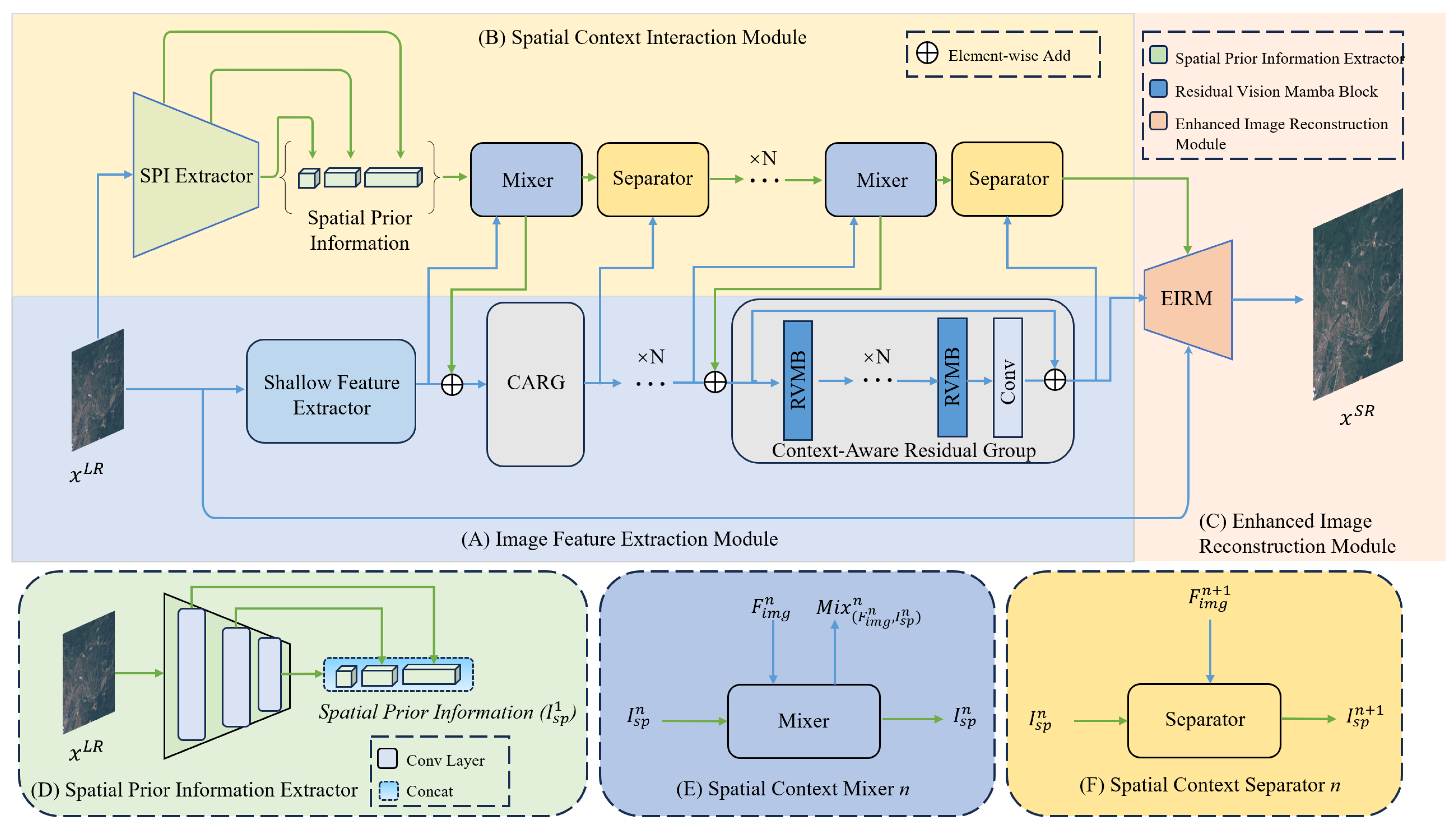
As shown in Figure 3, ESatSR consists of three parts: Image Feature Extraction Module, Spatial Context Interaction Module, and Enhanced Image Reconstruction Module. The Image Feature Extraction Module outputs shallow features and deep features of the image through the shallow feature extractor and multiple context-aware residual groups (CARGs). The Spatial Context Interaction Module acquires multi-scale spatial prior information from the LR image, then guides the feature extraction process through several sets of spatial context mixers and spatial context separators, and eventually outputs the spatial context required for restoring HR images. The Enhanced Image Reconstruction Module utilizes shallow features and deep features accompanied by spatial context, introduces residual connections from the front end of the Image Feature Extraction Module, and outputs high quality SR images. When the LR image is input into the model, it is divided into three streams: one flows through the Image Feature Extraction Module, one goes across the Spatial Context Interaction Module, and one enters into the residual connection. Streams are aggregated in the Enhanced Image Reconstruction Module and this then generates the SR image.

3.2. Image Feature Extraction Module

The Image Feature Extraction Module consists of two parts: the shallow feature extractor and deep feature extractor, where the latter is composed of sets of Context-Aware Residual Groups (CARGs). Given an LR image I l q R H × W × C that needs super-resolution, where H, W, and C represent the image’s height, width, and number of channels, we directly apply the shallow feature extractor, which is a 3 × 3 convolutional layer that transforms the input from image dimension into feature dimension. The process can be defined by the following formula:
S F = h s f e ( I l q ) , S F R H × W × D
where D is the number of feature channels in the network. h s f e ( · ) represents the 3 × 3 convolution. We added a convolutional layer here to leverage its capability in extracting local features. After that, we combined the shallow feature S F with the spatial context I s p 1 and fed them into Context-Aware Residual Groups (CARGs) to obtain deep feature F i m g 1 R H × W × D . This process can be described as:
F i m g 1 = h c a r g 1 ( S F , I l q 1 )
where h c a r g 1 represents the first context-aware residual group C A R G 1 , which contains N Residual Vision Mamba Blocks (RVMB), a 3 × 3 convolutional layer, and a residual connection. Spatial context I l q 1 is fused with image feature through element-wise addition. We define the intermediate variables that are output by N RVMBs as f 1 , f 2 , , f n , f 1 n R H × W × D , the process of outputting F i m g 1 from S F and I l q 1 is as follows:
f 1 = h r v m b 1 ( S F + I s p 1 )
f i = h r v m b i ( f i 1 ) , i = 1 , 2 , , N
F i m g 2 = h c o n v ( f N ) + S F + I s p 1
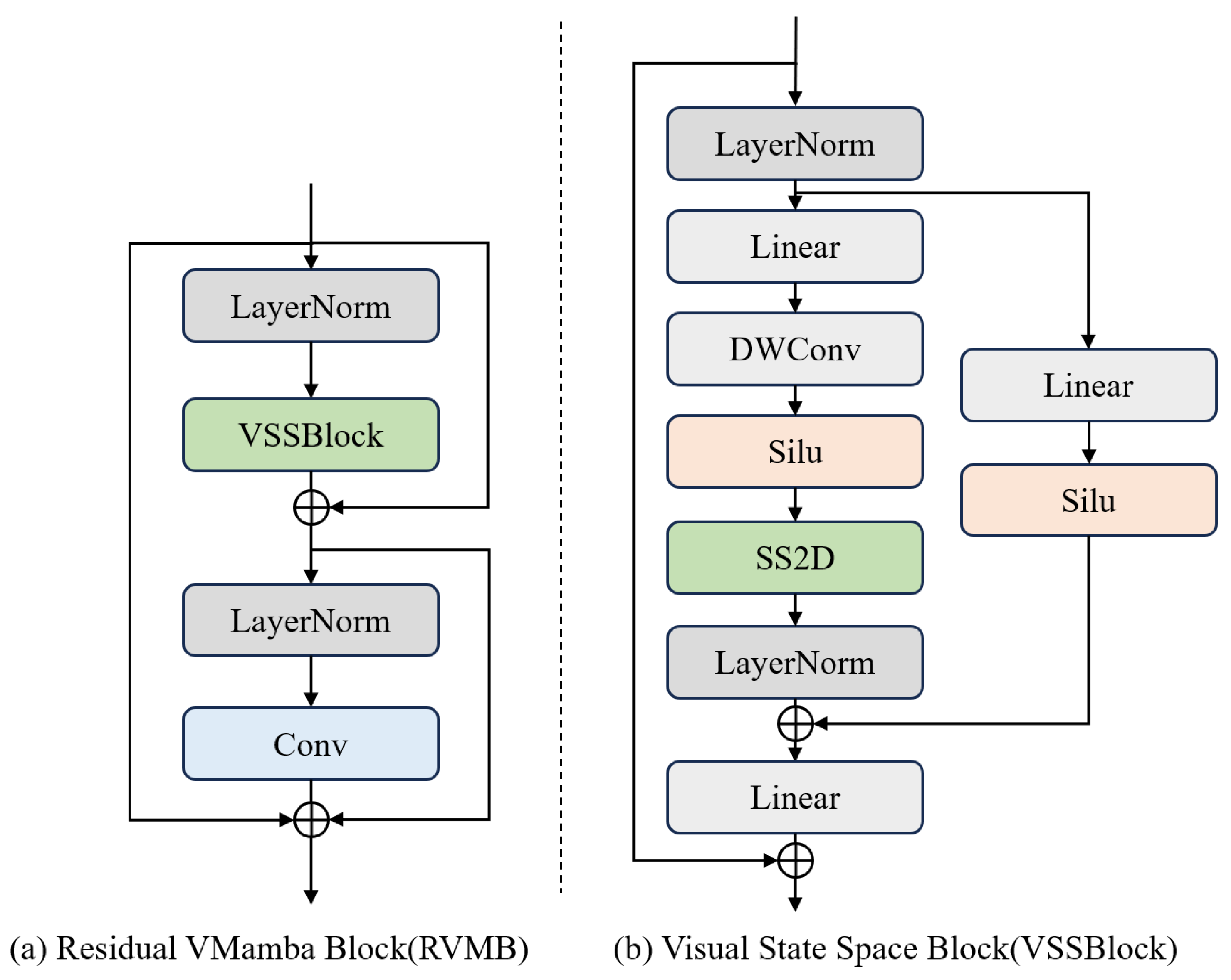
where h r v m b i is the i t h RVMB, and h c o n v is the convolution at the end of CARG. The architecture of RVMB is shown in Figure 4a, which includes two LayerNorms, a VSSBlock, a convolution layer, and multiple residual connections. Given an input f i n R H × W × D , we input it into the LayerNorm and the following VSSBlock. The VSSBlock is a core module in [21], and we introduced it into our network as an alternative to the self-attention computation of regular Transformers. The process of generating f o u t from f i n in RVMB can be summarized as
f m i d = h v s s b ( L N ( f i n ) ) + f i n
f o u t = h c o n v ( L N ( f m i d ) ) + f i n + f m i d
where LN means LayerNorm, and h v s s b represents the VSSBlock. The structure of the VSSBlock is shown in Figure 4b; its input will be divided into two branches: One will go through a 3 × 3 depth convolution, a Silu activation function, and an SS2D module. After the output of SS2D is passed through a LayerNorm, another branch is added to the existing one. This branch consists of a linear layer followed by a Silu activation function. The outputs of these two branches are combined to produce the result of the VSSBlock. Given the input S i n p u t R H × W × D , the output S o u t can be described as
s 1 = L N ( S S 2 D ( S i l u ( D W C o n v ( L i n e a r ( L N ( S i n p u t ) ) ) ) ) )
s 2 = S i l u ( L i n e a r ( L N ( S i n p u t ) ) )
S o u t = s 1 + s 2 + S i n p u t
where L i n e a r represents a linear layer, D W C o n v represents a depth-wise convolution with a kernel size of 3 × 3, and S S 2 D is a 2D Selective Scan module (SS2D). We introduce the SS2D of [21] into our network. Since vanilla mamba [47] was designed for 1D sequences, it cannot directly process 2D image data. Experiments show that it does not achieve considerable results if images were directly flattened into 1D tokens like what ViTs do to images. This is due to the direction sensitivity of mamba, which causes the model’s receptive field to be severely limited [21]. The SS2D module makes vanilla mamba more suitable for image data based on prior knowledge of computer vision. Specifically, instead of directly flattening the image, SS2D scans the image from four directions and obtains four 1D sequences: upper left to lower right, upper right to lower left, lower left to upper right, and lower right to upper left. Sequences processed in this way contain position information of each direction. Then each sequence will perform attention computation through an S6 Block [47], respectively. Finally, these four outputs are aggregated as the 2D image features. Eventually, after N CARGs, we can obtain the final deep features as
F i m g N = h c a r g n ( F i m g N 1 , I s p N )
The deep features F i m g n can then be utilized by the Enhanced Image Reconstruction Module to produce SR images.

3.3. Spatial Context Interaction Module

Inspired by [48], we used convolution to introduce spatial local information into our network. We designed a Spatial Context Interaction Module to introduce image-related prior knowledge. Meanwhile, we noticed that processing features across different scales allows the model to acquire the capability of effectively capturing small targets [49]. Therefore, we designed the spatial context to be in a multi-scale fashion. The Spatial Context Interaction Module contains a spatial prior information extractor (SPIE), N spatial context mixers (SCM), and N spatial context separators (SCS). SCM and SCS are arranged in a crosswise manner. An SCM with the following SCS can be regarded as a group, and each group has a corresponding Context-Aware Residual Group (CARG).
Initially, the spatial prior information acquired by the SPIE enters the first SCM, together with image features processed by the shallow feature extractor. The SCM mixes spatial context and image features, and passes the fused feature to the corresponding CARG. The SCS obtains the output of CARGs as references and updates spatial context by separating information from the former spatial context and references. In the end, the spatial context output by the last SCS is used by the Enhanced Image Reconstruction Module to help generate high-quality SR images.

3.3.1. Spatial Prior Information Extractor

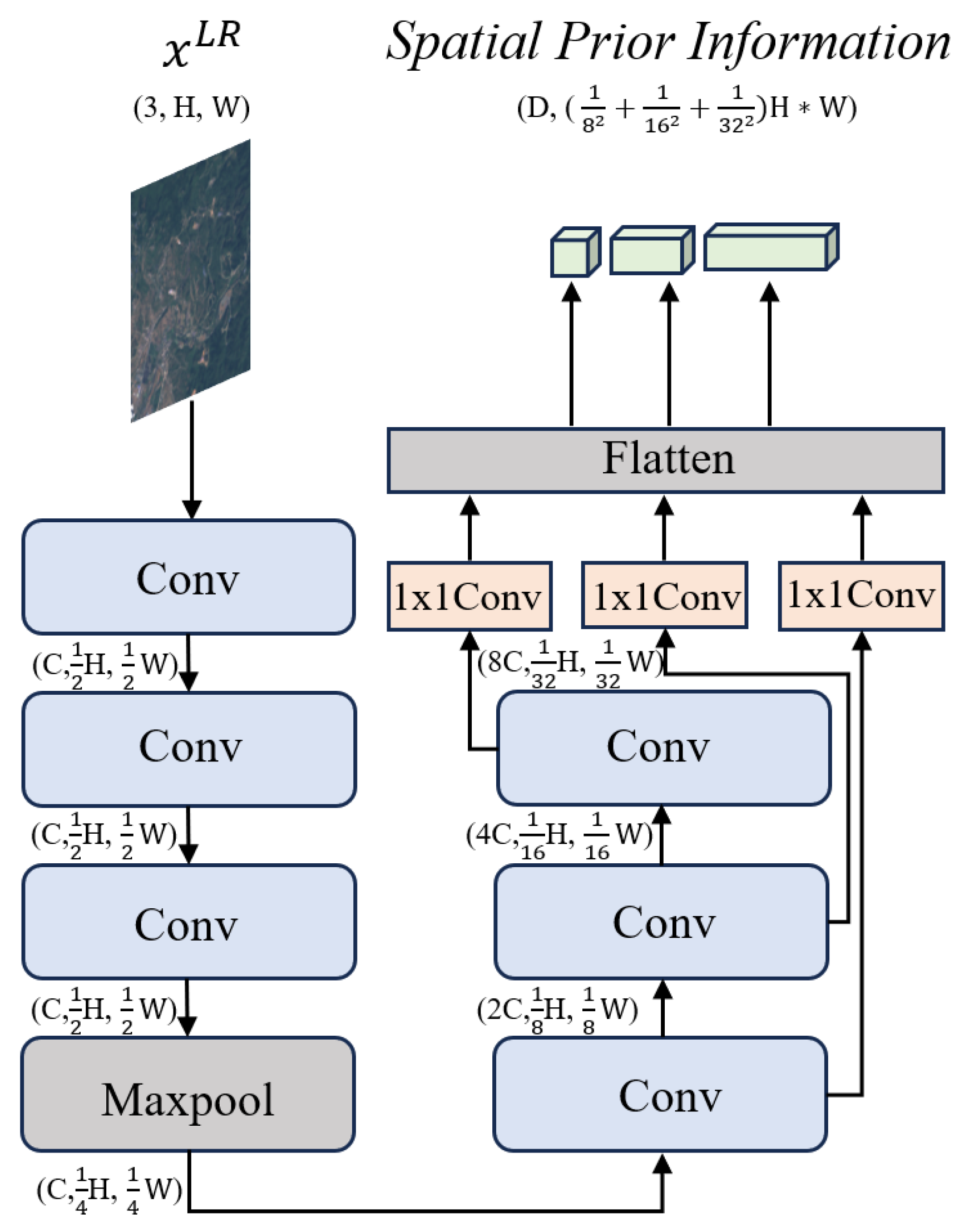
The architecture of the spatial prior information extractor (SPIE) is shown in Figure 5. Through SPIE, we extracted the raw spatial prior information from the LR image. Given the channel number of feature D and the input image I l q R ( 3 × H × W ) , we initially used three 3 × 3 convolutions and a max pooling layer to extract spatial features, and then used three 3 × 3 convolutions with stride 2 and kernel size 3 to increase channel numbers and reduce the size of the feature map. The output of each convolution is mapped from the original spatial feature dimension to the spatial contextual dimension D through a 1 × 1 convolution.
In order to interact with the Image Feature Extraction Module, we flattened the spatial contextual information of three different scales into three 1D sequences and concatenated them together to obtain the spatial prior information I s p 1 . Since each convolution reduces the size of feature maps by half, we can obtain the spatial contextual information at the scales of 1 8 , 1 16 , and 1 32 . The shape of concatenated spatial prior information I s p 1 can be noted as ( D , ( 1 8 2 + 1 16 2 + 1 32 2 ) H W ) . I s p 1 is then passed to the spatial context mixer, participating in the interaction between spatial context and image feature.

3.3.2. Spatial Context Mixer

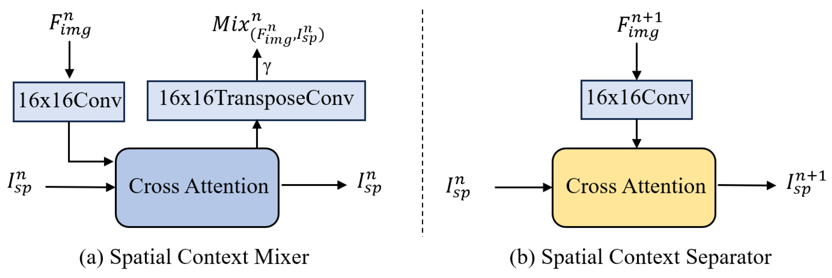
As shown in Figure 6a, the Spatial Context Mixer (SCM) conducts the fusion of fine-grained spatial context and image features through cross attention. For the n t h SCM, we take the output I s p n of the n 1 t h SCS as the key and value in the attention computation. Then, a 16 × 16 convolution is used to obtain patches of image feature as the query. Given image feature F i m g n R H × W × D and spatial context I s p n R ( 1 8 2 + 1 16 2 + 1 32 2 ) × D , the mixing process between spatial context and image feature can be described as:
M i x ( F i m g n , I s p n ) n = γ · h t r a n s c o n v ( C r o s s A t t e n t i o n ( h c o n v ( F i m g n ) , I s p n ) )
where h c o n v is a 16 × 16 convolution, extracting patches of size ( 1 16 H , 1 16 W ) . h t r a n s c o n v is a 16 × 16 transpose convolution, which aims to keep the output’s size consistent with image features. C r o s s A t t e n t i o n is the calculation of cross attention. Sparse attention is used here to reduce the complexity of the computation. Finally, since the mixed information is directly added to the original image feature, we use a learnable parameter γ to control the weight of the mixed information.

3.3.3. Spatial Context Separator

Figure 6b shows the architecture of Spatial Context Separator (SCS). It attempts to update spatial context by separating information from image features and previous spatial context. SCS also includes a cross attention computation. Different from SCM, SCS will use the image feature processed by CARG as the reference, and use the spatial context as the query to update spatial context for the next SCM. For the n t h SCS, the spatial context I s p n is the query, and the image features output by the corresponding CARG will go through a 16 × 16 convolution then serve as the key and value. Given image features F i m g n R H × W × D and spatial context I s p n R ( 1 8 2 + 1 16 2 + 1 32 2 ) × D , the process of producing the updated spatial context I s p n + 1 can be summarized as:
I s p n + 1 = I s p n + C r o s s A t t e n t i o n ( I s p n , h c o n v ( F i m g n ) )
where h c o n v is a 16 × 16 convolution, extracting patches of size ( 1 16 H , 1 16 W ) . Unlike SCM, the result of attention computation is directly added to the previous spatial context. This is because the jitter of image features will significantly affect the quality of image reconstruction. Therefore, we carefully control the changing of image features while applying a normal influence on the spatial context.

3.4. Enhanced Image Restoration Module

The workflow of the Enhanced Image Reconstruction Module is shown in Figure 7. Deep features and spatial context are used as the input of this module. The 1D spatial context is divided into three segments, with the length of 1 8 H W , 1 16 H W , and 1 32 H W . Then we rearrange these three segments into 2D feature maps z 1 , z 2 , and z 3 . A progressive upsample network is applied to these feature maps. To be specific, given the spatial context I s p n R ( D , ( 1 8 2 + 1 16 2 + 1 32 2 ) H W ) , we initially divide I s p n into three 1D sequences with the ratio of 4:2:1, and the sequences are z 1 = ( D , 1 8 2 H W ) , z 2 = ( D , 1 16 2 H W ) ) , and z 3 = ( D , 1 32 2 H W ) . Then z 1 , z 2 , and z 3 are sequentially scanned and rearranged into 2D feature maps z 1 = ( D , 1 8 H , 1 8 W ) , z 2 = ( D , 1 16 H , 1 16 W ) , and z 3 = ( D , 1 32 H , 1 32 W ) . z 3 is upsampled by a factor of two, and element-wisely added to z 2 to obtain z m i d . z m i d is then upsampled by a factor of two, and then added to z 1 to obtain z o u t R ( D , 1 8 H , 1 8 W ) . z o u t integrates spatial context of three scales and can compensate for fine-grained information of multiple scales for image restoration. We upsample feature maps through a PixelShuffle and a convolution. The process of obtaining output z o u t from input I s p n can be expressed by the following formula:
z 1 , z 2 , z 3 = s p l i t ( I s p n )
z 1 , z 2 , z 3 = u n e m b e d ( z 1 ) , u n e m b e d ( z 2 ) , u n e m b e d ( z 3 )
z o u t = h 2 x ( h 2 x ( z 3 ) + z 2 ) + z 1
where s p l i t ( · ) means splitting the spatial context according to the ratio of 4:2:1. u n e m b e d ( · ) represents the restoration of 1D spatial context into 2D feature maps. h 2 x represents upsampling by a factor of 2 through a convolution and a PixelShuffle. Then the deep feature F i m g N , the multi-scale spatial context z o u t , and the LR image input x L R are added, upsampled to the target image shape and transferred from the feature dimension to the image dimension. This process can be expressed as
x S R = h c o n v 2 ( h ( h c o n v 1 ( F i m g N + α z o u t + β x L R ) ) )
where α and β are the learnable weights that control the proportion of multi-scale spatial context z o u t and LR image input x L R during the reconstruction process. The feature is upsampled by h c o n v 1 and h . h c o n v 2 is the last layer of the network, which generates the reconstructed SR image x S R R ( 3 , H , W ) .

4. Experiments

In this section, we conduct a series of experiments to illustrate the performance of our model. ESatSR is compared against popular image restoration methods and SR models specifically designed for remote sensing images, including ECBSR, EDSR, RCAN, SwinIR, LGCNet, CTN, HSENet, EEGAN, and MHAN. These models are trained on DIV2K dataset and fine-tuned on OLI2MSI and RSSCN7, respectively. Then, we apply both qualitative and quantitative comparisons among them. In the end, an ablation study is set to find the impact of the number of modules on model performance, and delve into the effectiveness of Spatial Context Interaction Module and Enhanced Image Reconstruction Module.

4.1. Datasets

We performed our experiments on three public datasets, as follows:
  • DIV2K [50]: The DIV2K dataset includes 800 training images, 100 validation images, and 100 test images, all of which have 2K resolution. We divided the images into 480 × 480 sub-images with non-overlapping regions, and obtained LR images through bicubic downsampling.
  • OLI2MSI [51]: The OLI2MSI is a real-world remote sensing image dataset, containing 5225 training LR-HR image pairs and 100 test LR-HR image pairs. The HR images have 480 × 480 resolution and the LR images have a resolution of 180 × 180. The LR images are ground images with a spatial resolution of 30 m, captured by the Operational Land Imager Landsat-8 satellite, and the HR images are ground images with a spatial resolution of 10 m, captured by the Multispectral Instrument Sentinel-2 satellite. Since the original scale factor of the dataset is 3, we used bicubic to obtain LR images for other scale factors.
  • RSSCN7 [52]: The RSSCN7 contains 2800 remote sensing images collected from Google Earth, covering various classic remote sensing scenarios, including grasslands, forests, fields, lakes, parking lots, residential areas, and factory areas. Bicubic is used here to generate corresponding LR images.
The models were initially trained on the DIV2K dataset, and then fine-tuned on OLI2MSI and RSSCN7 datasets, respectively. For OLI2MSI, we used the 100 test LR-HR image pairs to assess model performance. For RSSCN7, we divided the dataset into training set, validation set, and test set in a ratio of 7:2:1, and the model was evaluated on the test set.

4.2. Comparison Methods

To evaluate the performance of ESatSR, we conducted comparisons with several state-of-the-art super-resolution algorithms, including four image restoration methods and five SR algorithms tailored for remote sensing images, as follows:
  • ECBSR [53]: ECBSR is a lightweight SR model built with ECB, which is an improved convolution block. After replacing simple convolutional layers with ECB, the model’s inference is sped up, and the performance is also comparable to the popular SR methods.
  • EDSR [25]: Based on SRResNet [9], EDSR removes the redundant BatchNorms and simplifies the network structure, which enables the network to be deeper and contributes to improved performance.
  • RCAN [20]: RCAN proposes a Residual-in-Residual module that can be used to build a deeper residual network. A channel attention mechanism is also added to RCAN to enhance the representation ability.
  • SwinIR [16]: Introducing shifted window into the field of image restoration, SwinIR utilizes the attention among windows to enhance its local feature extraction capability, demonstrating state-of-the-art performance.
  • LGCNet [36]: LGCNet fuses the outputs of different convolutional layers, which can improve the quality of SR images.
  • CTN [37]: CTN extracts image features through a hierarchical architecture. Through a context aggregation module, the features are enhanced and combined to reconstruct SR images.
  • HSENet [40]: An observation of remote sensing images is that lots of similar targets usually occur concurrently. To take advantage of that, HSENet designed a self-similarity utilization module to calculate the correlation of features at the same scale. Residual connections are set so that the network can refer to the features of similar targets in other scales during image reconstruction.
  • EEGAN [54]: The usual GAN-based method produces a high-resolution result that looks sharp but is eroded with artifacts and noises. EEGAN uses edge-enhancement sub-networks to extract and enhance the image contours by purifying the noise-contaminated components with mask processing. The contours and purified image are combined to generate the final SR output.
  • MHAN [55]: MHAN consists of two sub-networks bridged by a frequency-aware connection. One network is responsible for feature extraction, and it replaces the element-wise addition with weighted channel-wise concatenation in all skip connections, greatly facilitating the flow of information. The other network introduces a high-order attention module instead of the usual spatial or channel attention to restore missing details. MHAN exhibits superior performance among various SR methods tailored for remote sensing images.

4.3. Implementation Details

All experiments were implemented with Pytorch [56] framework and run on a NVIDIA RTX 3090 GPU. We applied data augmentation on datasets, including horizontal flipping and random rotations of 90°, 180°, and 270°. Then we cropped the image into 64 × 64 patches for super-resolution. We calculated FLOPs and the number of parameters when the size of HR was fixed to 384 × 384. The batch size was set to 8 for fair comparisons among different methods. The channel number is 180. The Adam optimizer [57] was applied with β 1 = 0.9 and β 2 = 0.999 . The initial learning rate is 2 × 10 4 and is halved when the training process reaches 1 2 , 3 4 and 7 8 . We trained all models for 50 epochs. The number of context-aware residual groups (CARGs) is set to six, and each CARGs consists of six RVMBs. Every CARG has a corresponding group, which contains a spatial context mixer and a spatial context separator.

4.4. Quantitative and Qualitative Comparisons

We conducted experiments on the OLI2MSI and RSSCN7 datasets. PSNR [58], SSIM [58], and LPIPS [59] were employed as metrics to evaluate performance for methods mentioned above. All methods were developed for both scale factor 2 and scale factor 3, respectively.
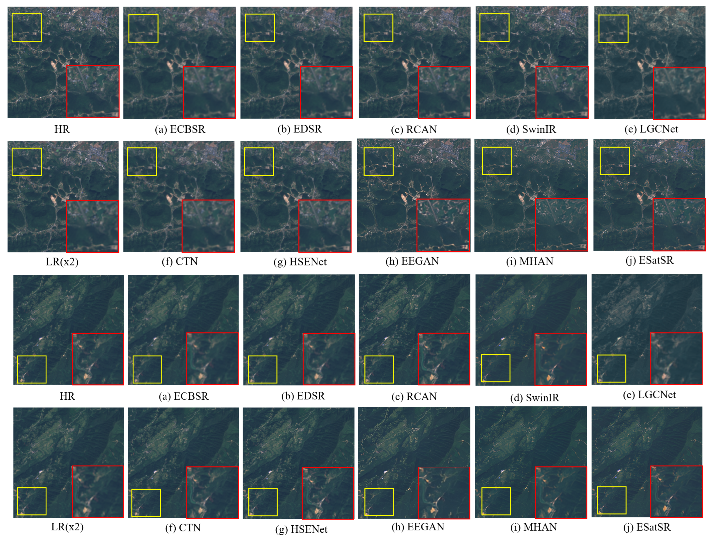
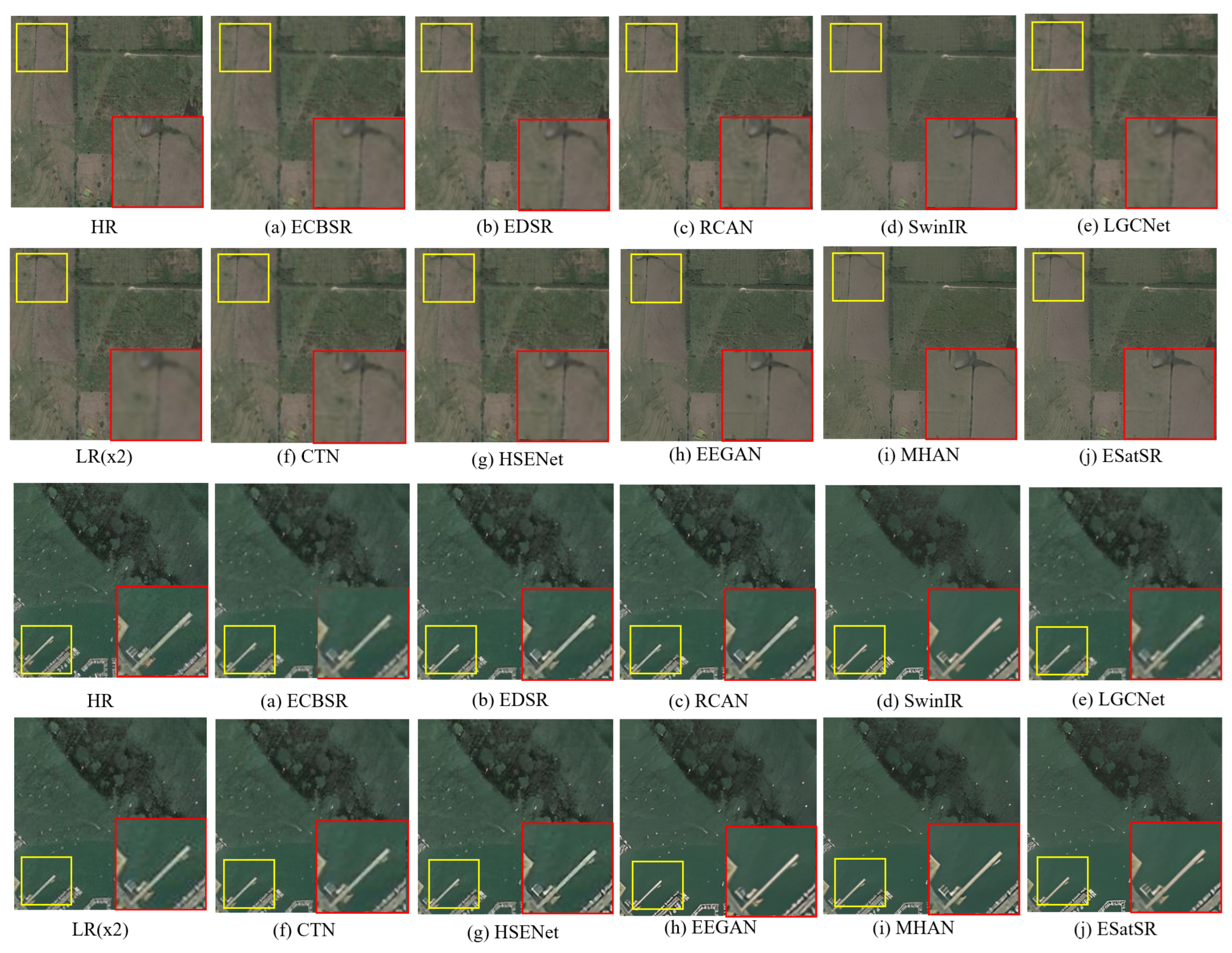
Table 1 shows the quantitative results of ESatSR and other comparison methods with a scale factor of 2. As can be seen, when trained on DIV2K and fine-tuned on OLI2MSI or RSSCN7, ESatSR demonstrates the best performance among all compared methods, with 31.4243 dB PSNR and 0.8267 dB SSIM on RSSCN7 and 42.1131 dB PSNR and 0.9784 SSIM on OLI2MSI. The PSNR gain achieved is 0.22 dB on RSSCN7. All CNN-based methods perform worse than ESatSR and SwinIR, while SwinIR shows sub-optimal performance in all methods. Qualitative comparisons are shown in Figure 8 and Figure 9. Due to the content-irrelevant convolution, most CNN-based methods generate blurry and noisy images. SwinIR produces better images compared to CNN-based methods; however, it suffers from the limitation of receptive fields, resulting in a slightly blurry border. ESatSR utilizes multi-scale spatial context to restore fine-grained high-frequency details, which contributes to images with sharper and clearer edges.
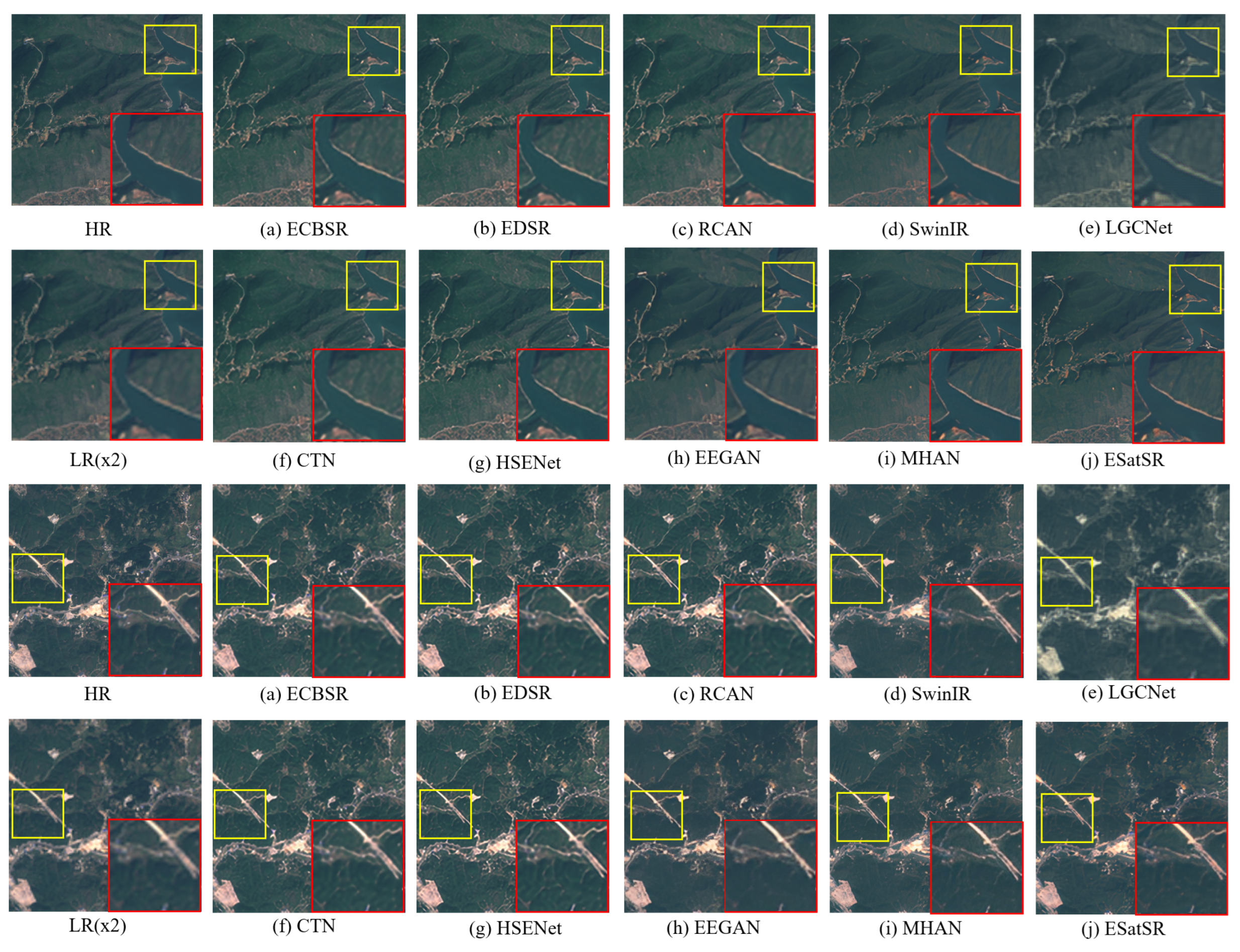
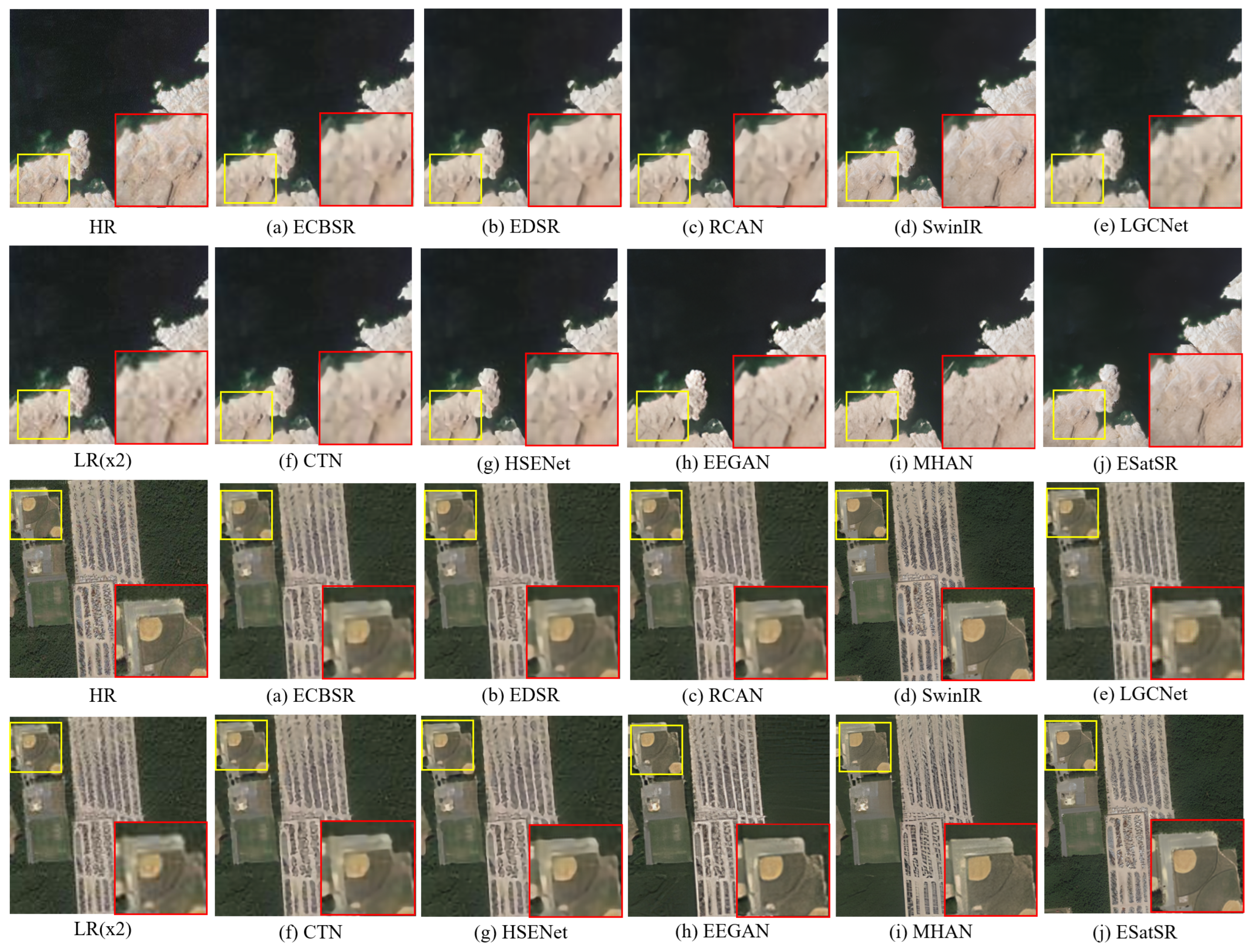
Table 2 shows the quantitative results of ESatSR and other methods with a scale factor of 3. Because OLI2MSI ×3 is a real-world dataset, the degradation of images is more complex and each method shows a significant decrease in metrics. Despite that, ESatSR still achieves the best performance, with 29.2552 dB PSNR and 0.7262 dB SSIM on RSSCN7 and 35.1744 dB PSNR and 0.9276 SSIM on OLI2MSI. The PSNR gain reaches 0.27 dB on OLI2MSI. SwinIR produces the sub-optimal result. CTN and HSENet outperform some image restoration methods on OLI2MSI ×3, which may be attributed to their modules tailored for remote sensing images, enhancing their performance on real-world datasets. Qualitative comparisons are shown in Figure 10 and Figure 11. Even though the scale factor is larger, ESatSR can obtain images with detailed texture and sharp edges, while most CNN-based methods suffer from blur and unsatisfactory artifacts. And SwinIR, as the sub-optimal method, produces competitive images with slight blurring and distortions.

4.5. Ablation Studies

For ablation studies, ESatSR was trained on DIV2K and fine-tuned on OLI2MSI. The scale factor was set to 2, and the evaluation was conducted on test images of OLI2MSI with PSNR and SSIM as the metrics.

4.5.1. The Effectiveness of Spatial Context Interaction Module

We delved into the contribution of each design, including the Spatial Prior Information Extractor (SPIE), Spatial Context Mixer, and Spatial Context Separator of Spatial Context Interaction Module (SCIM). As is shown in Table 3, simply employing RVMBs results in performance similar to SwinIR. By introducing the spatial prior, Variant 1 achieves a slight improvement. Variant 2 applies spatial context mixers to enhance image features, which improves performance by 0.08 PSNR. From Variant 3, we can see that the separators are added and gain 0.04 PSNR, which demonstrates the effectiveness of updating spatial context along with image features concurrently. In conclusion, by applying SCIM, our method gains an improvement of 0.13 PSNR.

4.5.2. The Effectiveness of Enhanced Image Reconstruction Module and the Multi-Scale Design of Spatial Context

The Enhanced Image Reconstruction Module (EIRM) utilizes spatial context from SCIM. As is shown in Table 3, there are two settings of EIRM. “Single” means EIRM is not activated, and only the coarsest spatial context at 1 8 scale is used across the network. “Multi” means EIRM is applied and multi-scale fine-grained spatial context will be utilized. It can be concluded from the results that, compared to Variant 3, our ESatSR uses spatial context of all scales through progressively upsampling, and boosts the performance by 0.03 PSNR. This demonstrates that the multi-scale design of spatial context will enhance the model’s ability of extracting features of small objects, and the effectiveness of EIRM has also been proven.

4.5.3. The Impact of Channel Number, RVMB Number, and CARG Number

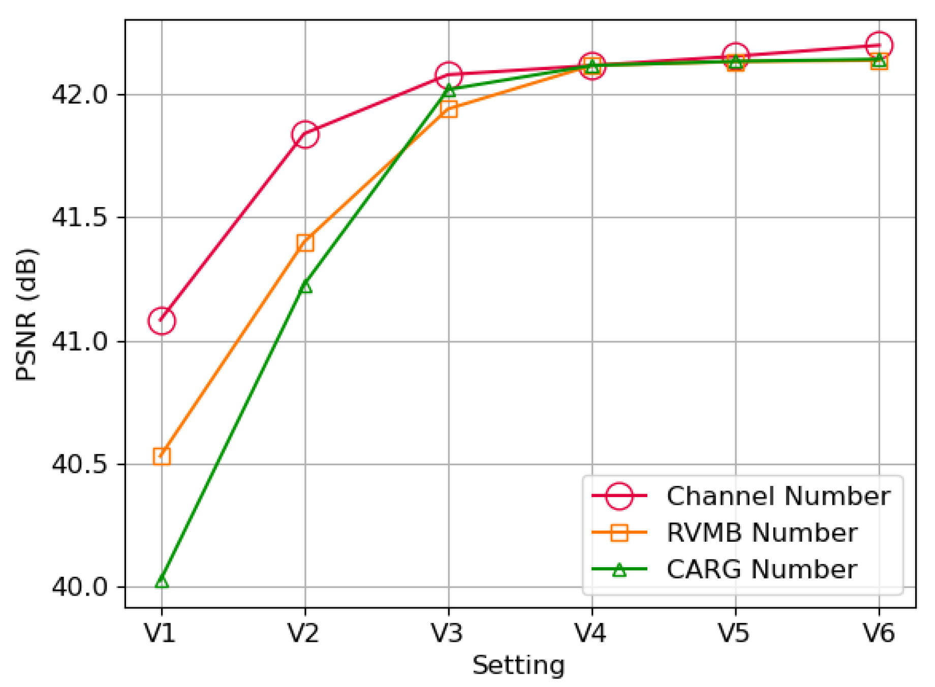
The impact of channel number, RVMB number, and CARG number on the model’s performance is demonstrated in Figure 12 and Table 4. It can be concluded that the PSNR is mainly positively correlated with these hyperparameters. The performance shows a consistent improvement with the increase in channel number. For RVMB number and CARG number, the PSNR tends to increase gradually with RVMB and CARG numbers growing and then reaches a plateau. To balance model size and performance, we select 180 as the channel number of our model, though performance will continue to improve if more channels could be used. With the observation that the performance becomes saturated if RVMB number and CARG number keep growing, we choose six RVMBs for each CARG and six CARGs in total to maintain a relatively reasonable model size.

5. Discussion

We introduced 2D Selective Scan to SR methods for remote sensing images, and exploited spatial context for further enhancement. Previous CNN-based methods suffer from a limited receptive field, resulting in blur and artifacts in images (Figure 8, Figure 9, Figure 10 and Figure 11). SwinIR has a wide receptive field due to the efficacy of self-attention mechanism. However, lacking prior assumptions, it shows inferior performance in downstream dense prediction tasks and produces sub-optimal results in our experiments. By introducing SS2D as an alternative to the Transformer’s attention mechanism, ESatSR can obtain an extensive receptive field similar to Transformers, and gains an enhanced capability in modeling long-range dependencies [21]. Meanwhile, we designed the SCIM to introduce image-related prior knowledge, addressing the lack of prior assumptions. Multi-scale spatial context interacts with image features to compensate for information of small objects.The EIRM is applied to utilize spatial context to restore images. By applying these enhancements, ESatSR demonstrates superior performance to other methods, as illustrated in Table 1 and Table 2. A series of ablation studies were conducted and the results are shown in Table 3 and Figure 12, demonstrating the effectiveness of SCIM and EIRM.
While introducing spatial context brings performance improvements, the interaction between spatial context and image features needs to be optimized. To save the computational cost of cross attention, we applied a 16 × 16 convolution to extract image features into patches. Then, the result of cross attention was restored to their original shape by a 16 × 16 transpose convolution. This process of convolution and transpose convolution would inevitably hinder the representation of spatial context, leading to reduced performance. Meanwhile, the model’s capability to handle real-world degradation has not been explored. A network modeling complex degradation could be used as a prior module for our methods, adapting the model to real-world datasets. Moreover, our experiments focus on remote sensing images due to task requirements. Future research can be conducted for general images to demonstrate the robustness and generalization ability of ESatSR.

6. Conclusions

In this paper, we propose a novel SR method for remote sensing images, named ESatSR, to address the limitations of previous SR works, including limited receptive fields and the lack of prior assumptions, while leveraging the multi-scale spatial context to enable our method effectively capturing features of small targets in satellite remote sensing images. ESatSR consists of three parts, the Image Feature Extraction Module, Spatial Context Interaction Module, and Enhanced Image Reconstruction Module. Extensive experiments on various datasets show that ESatSR can produce high-quality SR images and achieve state-of-the-art performance. In the future, our work will focus on designing an efficient cross attention mechanism for spatial context interaction. We will also improve the model’s capability to restore images with unknown degradation, exploring the potential of state space model in real-world image SR tasks. Our code and models will be released at https://github.com/Yosagai/ESatSR (accessed on 28 May 2024).

Author Contributions

Conceptualization, Y.W. and W.Y.; methodology, Y.W. and W.Y.; software, Y.W.; validation, Y.W.; formal analysis, Y.W. and W.Y.; investigation, Y.W.; data curation, Y.W.; writing—original draft preparation, Y.W.; writing—review and editing, W.Y.; visualization, Y.W.; supervision, F.X. and B.L.; project administration, B.L. All authors have read and agreed to the published version of the manuscript.

Funding

This research received no external funding.

Data Availability Statement

The original data presented in the study are openly available at [50,51,52].

Conflicts of Interest

The authors declare no conflicts of interest.

References

  1. Li, Q.; Gong, H.; Dai, H.; Li, C.; He, Z.; Wang, W.; Feng, Y.; Han, F.; Tuniyazi, A.; Li, H.; et al. Unsupervised hyperspectral image change detection via deep learning self-generated credible labels. IEEE J. Sel. Top. Appl. Earth Obs. Remote Sens. 2021, 14, 9012–9024. [Google Scholar] [CrossRef]
  2. Gong, M.; Jiang, F.; Qin, A.K.; Liu, T.; Zhan, T.; Lu, D.; Zheng, H.; Zhang, M. A spectral and spatial attention network for change detection in hyperspectral images. IEEE Trans. Geosci. Remote Sens. 2021, 60, 1–14. [Google Scholar] [CrossRef]
  3. Wang, Y.; Bashir, S.M.A.; Khan, M.; Ullah, Q.; Wang, R.; Song, Y.; Guo, Z.; Niu, Y. Remote sensing image super-resolution and object detection: Benchmark and state of the art. Expert Syst. Appl. 2022, 197, 116793. [Google Scholar] [CrossRef]
  4. Gong, H.; Mu, T.; Li, Q.; Dai, H.; Li, C.; He, Z.; Wang, W.; Han, F.; Tuniyazi, A.; Li, H.; et al. Swin-transformer-enabled YOLOv5 with attention mechanism for small object detection on satellite images. Remote Sens. 2022, 14, 2861. [Google Scholar] [CrossRef]
  5. Ngo, T.D.; Bui, T.T.; Pham, T.M.; Thai, H.T.; Nguyen, G.L.; Nguyen, T.N. Image deconvolution for optical small satellite with deep learning and real-time GPU acceleration. J. Real-Time Image Process. 2021, 18, 1697–1710. [Google Scholar] [CrossRef]
  6. Ye, Y.; Yang, C.; Gong, G.; Yang, P.; Quan, D.; Li, J. Robust optical and SAR image matching using attention-enhanced structural features. IEEE Trans. Geosci. Remote Sens. 2024, 62, 1–12. [Google Scholar] [CrossRef]
  7. Zhao, Q.; Dong, L.; Liu, M.; Kong, L.; Chu, X.; Hui, M.; Zhao, Y. Visible/Infrared Image Registration Based on Region-Adaptive Contextual Multi-Features. IEEE Trans. Geosci. Remote Sens. 2024, 62, 1–17. [Google Scholar]
  8. Dong, C.; Loy, C.C.; He, K.; Tang, X. Image super-resolution using deep convolutional networks. IEEE Trans. Pattern Anal. Mach. Intell. 2015, 38, 295–307. [Google Scholar] [CrossRef]
  9. Ledig, C.; Theis, L.; Huszár, F.; Caballero, J.; Cunningham, A.; Acosta, A.; Aitken, A.; Tejani, A.; Totz, J.; Wang, Z.; et al. Photo-realistic single image super-resolution using a generative adversarial network. In Proceedings of the IEEE Conference on Computer Vision and Pattern Recognition (CVPR), Honolulu, HI, USA, 21–26 July 2017; pp. 4681–4690. [Google Scholar]
  10. Kim, J.; Lee, J.K.; Lee, K.M. Accurate image super-resolution using very deep convolutional networks. In Proceedings of the IEEE Conference on Computer Vision and Pattern Recognition (CVPR), Las Vegas, NV, USA, 27–30 June 2016; pp. 1646–1654. [Google Scholar]
  11. Zhang, K.; Zuo, W.; Gu, S.; Zhang, L. Learning deep CNN denoiser prior for image restoration. In Proceedings of the IEEE Conference on Computer Vision and Pattern Recognition (CVPR), Honolulu, HI, USA, 21–26 July 2017; pp. 3929–3938. [Google Scholar]
  12. Dosovitskiy, A.; Beyer, L.; Kolesnikov, A.; Weissenborn, D.; Zhai, X.; Unterthiner, T.; Dehghani, M.; Minderer, M.; Heigold, G.; Gelly, S.; et al. An image is worth 16x16 words: Transformers for image recognition at scale. arXiv 2020, arXiv:2010.11929. [Google Scholar]
  13. Carion, N.; Massa, F.; Synnaeve, G.; Usunier, N.; Kirillov, A.; Zagoruyko, S. End-to-end object detection with transformers. In Proceedings of the European Conference on Computer Vision, Tel Aviv, Israel, 23–27 October 2022; Springer: Berlin/Heidelberg, Germany, 2020; pp. 213–229. [Google Scholar]
  14. Chen, H.; Wang, Y.; Guo, T.; Xu, C.; Deng, Y.; Liu, Z.; Ma, S.; Xu, C.; Xu, C.; Gao, W. Pre-trained image processing transformer. In Proceedings of the IEEE/CVF Conference on Computer Vision and Pattern Recognition, Nashville, TN, USA, 20–25 June 2021; pp. 12299–12310. [Google Scholar]
  15. Cao, J.; Li, Y.; Zhang, K.; Liang, J.; Van Gool, L. Video super-resolution transformer. arXiv 2021, arXiv:2106.06847. [Google Scholar]
  16. Liang, J.; Cao, J.; Sun, G.; Zhang, K.; Van Gool, L.; Timofte, R. Swinir: Image restoration using swin transformer. In Proceedings of the IEEE/CVF International Conference on Computer Vision (ICCV), Montreal, QC, Canada, 10–17 October 2021; pp. 1833–1844. [Google Scholar]
  17. Wang, W.; Xie, E.; Li, X.; Fan, D.P.; Song, K.; Liang, D.; Lu, T.; Luo, P.; Shao, L. Pvt v2: Improved baselines with pyramid vision transformer. Comput. Vis. Media 2022, 8, 415–424. [Google Scholar] [CrossRef]
  18. Xie, E.; Wang, W.; Yu, Z.; Anandkumar, A.; Alvarez, J.M.; Luo, P. SegFormer: Simple and efficient design for semantic segmentation with transformers. Adv. Neural Inf. Process. Syst. 2021, 34, 12077–12090. [Google Scholar]
  19. Chen, X.; Wang, X.; Zhou, J.; Qiao, Y.; Dong, C. Activating more pixels in image super-resolution transformer. In Proceedings of the IEEE/CVF Conference on Computer Vision and Pattern Recognition, Vancouver, BC, Canada, 17–24 June 2023; pp. 22367–22377. [Google Scholar]
  20. Zhang, Y.; Li, K.; Li, K.; Wang, L.; Zhong, B.; Fu, Y. Image super-resolution using very deep residual channel attention networks. In Proceedings of the European Conference on Computer Vision (ECCV), Munich, Germany, 8–14 September 2018; pp. 286–301. [Google Scholar]
  21. Liu, Y.; Tian, Y.; Zhao, Y.; Yu, H.; Xie, L.; Wang, Y.; Ye, Q.; Liu, Y. Vmamba: Visual state space model. arXiv 2024, arXiv:2401.10166. [Google Scholar]
  22. Dai, T.; Cai, J.; Zhang, Y.; Xia, S.T.; Zhang, L. Second-order attention network for single image super-resolution. In Proceedings of the IEEE/CVF Conference on Computer Vision and Pattern Recognition, Long Beach, CA, USA, 15–20 June 2019; pp. 11065–11074. [Google Scholar]
  23. Niu, B.; Wen, W.; Ren, W.; Zhang, X.; Yang, L.; Wang, S.; Zhang, K.; Cao, X.; Shen, H. Single image super-resolution via a holistic attention network. In Proceedings of the Computer Vision–ECCV 2020: 16th European Conference, Glasgow, UK, 23–28 August 2020; Part XII 16. Springer: Berlin/Heidelberg, Germany, 2020; pp. 191–207. [Google Scholar]
  24. Mei, Y.; Fan, Y.; Zhou, Y. Image super-resolution with non-local sparse attention. In Proceedings of the IEEE/CVF Conference on Computer Vision and Pattern Recognition, Virtually, 19–25 June 2021; pp. 3517–3526. [Google Scholar]
  25. Lim, B.; Son, S.; Kim, H.; Nah, S.; Mu Lee, K. Enhanced deep residual networks for single image super-resolution. In Proceedings of the IEEE Conference on Computer Vision and Pattern Recognition Workshops, Honolulu, HI, USA, 21–26 July 2017; pp. 136–144. [Google Scholar]
  26. Zhang, Y.; Tian, Y.; Kong, Y.; Zhong, B.; Fu, Y. Residual dense network for image super-resolution. In Proceedings of the IEEE Conference on Computer Vision and Pattern Recognition, Salt Lake City, UT, USA, 18–23 June 2018; pp. 2472–2481. [Google Scholar]
  27. Kim, J.; Lee, J.K.; Lee, K.M. Deeply-recursive convolutional network for image super-resolution. In Proceedings of the IEEE Conference on Computer Vision and Pattern Recognition, Las Vegas, NV, USA, 27–30 June 2016; pp. 1637–1645. [Google Scholar]
  28. Zhou, S.; Zhang, J.; Zuo, W.; Loy, C.C. Cross-scale internal graph neural network for image super-resolution. Adv. Neural Inf. Process. Syst. 2020, 33, 3499–3509. [Google Scholar]
  29. Wang, X.; Yu, K.; Wu, S.; Gu, J.; Liu, Y.; Dong, C.; Qiao, Y.; Change Loy, C. Esrgan: Enhanced super-resolution generative adversarial networks. In Proceedings of the European Conference on Computer Vision (ECCV) Workshops, Munich, Germany, 8–14 September 2019; pp. 63–79. [Google Scholar]
  30. Wang, X.; Xie, L.; Dong, C.; Shan, Y. Real-esrgan: Training real-world blind super-resolution with pure synthetic data. In Proceedings of the IEEE/CVF International Conference on Computer Vision, Montreal, BC, Canada, 11–17 October 2021; pp. 1905–1914. [Google Scholar]
  31. Touvron, H.; Cord, M.; Douze, M.; Massa, F.; Sablayrolles, A.; Jégou, H. Training data-efficient image transformers & distillation through attention. In Proceedings of the International Conference on Machine Learning. PMLR, Virtual Event, 18–24 July 2021; pp. 10347–10357. [Google Scholar]
  32. Cao, H.; Wang, Y.; Chen, J.; Jiang, D.; Zhang, X.; Tian, Q.; Wang, M. Swin-unet: Unet-like pure transformer for medical image segmentation. In Proceedings of the European Conference on Computer Vision, Tel Aviv, Israel, 23 October 2022; Springer: Berlin/Heidelberg, Germany, 2022; pp. 205–218. [Google Scholar]
  33. Wu, B.; Xu, C.; Dai, X.; Wan, A.; Zhang, P.; Yan, Z.; Tomizuka, M.; Gonzalez, J.; Keutzer, K.; Vajda, P. Visual transformers: Token-based image representation and processing for computer vision. arXiv 2020, arXiv:2006.03677. [Google Scholar]
  34. Zheng, S.; Lu, J.; Zhao, H.; Zhu, X.; Luo, Z.; Wang, Y.; Fu, Y.; Feng, J.; Xiang, T.; Torr, P.H.; et al. Rethinking semantic segmentation from a sequence-to-sequence perspective with transformers. In Proceedings of the IEEE/CVF Conference on Computer Vision and Pattern Recognition, Virtually, 19–25 June 2021; pp. 6881–6890. [Google Scholar]
  35. Liu, Z.; Lin, Y.; Cao, Y.; Hu, H.; Wei, Y.; Zhang, Z.; Lin, S.; Guo, B. Swin Transformer: Hierarchical Vision Transformer Using Shifted Windows. In Proceedings of the IEEE/CVF International Conference on Computer Vision (ICCV), Montreal, QC, Canada, 10–17 October 2021; pp. 10012–10022. [Google Scholar]
  36. Lei, S.; Shi, Z.; Zou, Z. Super-resolution for remote sensing images via local–global combined network. IEEE Geosci. Remote Sens. Lett. 2017, 14, 1243–1247. [Google Scholar] [CrossRef]
  37. Wang, S.; Zhou, T.; Lu, Y.; Di, H. Contextual transformation network for lightweight remote-sensing image super-resolution. IEEE Trans. Geosci. Remote Sens. 2021, 60, 1–13. [Google Scholar] [CrossRef]
  38. Gu, J.; Sun, X.; Zhang, Y.; Fu, K.; Wang, L. Deep residual squeeze and excitation network for remote sensing image super-resolution. Remote Sens. 2019, 11, 1817. [Google Scholar] [CrossRef]
  39. Wang, Z.; Li, L.; Xue, Y.; Jiang, C.; Wang, J.; Sun, K.; Ma, H. FeNet: Feature enhancement network for lightweight remote-sensing image super-resolution. IEEE Trans. Geosci. Remote Sens. 2022, 60, 1–12. [Google Scholar] [CrossRef]
  40. Lei, S.; Shi, Z. Hybrid-scale self-similarity exploitation for remote sensing image super-resolution. IEEE Trans. Geosci. Remote Sens. 2021, 60, 1–10. [Google Scholar] [CrossRef]
  41. Lei, S.; Shi, Z.; Mo, W. Transformer-based multistage enhancement for remote sensing image super-resolution. IEEE Trans. Geosci. Remote Sens. 2021, 60, 1–11. [Google Scholar] [CrossRef]
  42. Kalman, R.E. A new approach to linear filtering and prediction problems. Trans. ASME D 1960, 82, 35–44. [Google Scholar] [CrossRef]
  43. Gu, A.; Goel, K.; Ré, C. Efficiently modeling long sequences with structured state spaces. arXiv 2021, arXiv:2111.00396. [Google Scholar]
  44. Gu, A.; Johnson, I.; Goel, K.; Saab, K.; Dao, T.; Rudra, A.; Ré, C. Combining recurrent, convolutional, and continuous-time models with linear state space layers. Adv. Neural Inf. Process. Syst. 2021, 34, 572–585. [Google Scholar]
  45. Gupta, A.; Gu, A.; Berant, J. Diagonal state spaces are as effective as structured state spaces. Adv. Neural Inf. Process. Syst. 2022, 35, 22982–22994. [Google Scholar]
  46. Li, Y.; Cai, T.; Zhang, Y.; Chen, D.; Dey, D. What makes convolutional models great on long sequence modeling? arXiv 2022, arXiv:2210.09298. [Google Scholar]
  47. Gu, A.; Dao, T. Mamba: Linear-time sequence modeling with selective state spaces. arXiv 2023, arXiv:2312.00752. [Google Scholar]
  48. Wu, H.; Xiao, B.; Codella, N.; Liu, M.; Dai, X.; Yuan, L.; Zhang, L. Cvt: Introducing convolutions to vision transformers. In Proceedings of the IEEE/CVF International Conference on Computer Vision, Montreal, BC, Canada, 11–17 October 2021; pp. 22–31. [Google Scholar]
  49. Ghiasi, G.; Lin, T.Y.; Le, Q.V. Nas-fpn: Learning scalable feature pyramid architecture for object detection. In Proceedings of the IEEE/CVF Conference on Computer Vision and Pattern Recognition, Long Beach, CA, USA, 15–20 June 2019; pp. 7036–7045. [Google Scholar]
  50. Agustsson, E.; Timofte, R. Ntire 2017 challenge on single image super-resolution: Dataset and study. In Proceedings of the IEEE Conference on Computer Vision and Pattern Recognition Workshops, Honolulu, HI, USA, 21–26 July 2017; pp. 126–135. [Google Scholar]
  51. Wang, J.; Gao, K.; Zhang, Z.; Ni, C.; Hu, Z.; Chen, D.; Wu, Q. Multisensor remote sensing imagery super-resolution with conditional GAN. J. Remote Sens. 2021, 2021, 9829706. [Google Scholar] [CrossRef]
  52. Zou, Q.; Ni, L.; Zhang, T.; Wang, Q. Deep Learning Based Feature Selection for Remote Sensing Scene Classification. IEEE Geosci. Remote Sens. Lett. 2015, 12, 2321–2325. [Google Scholar] [CrossRef]
  53. Zhang, X.; Zeng, H.; Zhang, L. Edge-oriented convolution block for real-time super resolution on mobile devices. In Proceedings of the 29th ACM International Conference on Multimedia, Virtual Event, 20–24 October 2021; pp. 4034–4043. [Google Scholar]
  54. Jiang, K.; Wang, Z.; Yi, P.; Wang, G.; Lu, T.; Jiang, J. Edge-enhanced GAN for remote sensing image superresolution. IEEE Trans. Geosci. Remote Sens. 2019, 57, 5799–5812. [Google Scholar] [CrossRef]
  55. Zhang, D.; Shao, J.; Li, X.; Shen, H.T. Remote Sensing Image Super-Resolution via Mixed High-Order Attention Network. IEEE Trans. Geosci. Remote Sens. 2021, 59, 5183–5196. [Google Scholar] [CrossRef]
  56. Paszke, A.; Gross, S.; Massa, F.; Lerer, A.; Bradbury, J.; Chanan, G.; Killeen, T.; Lin, Z.; Gimelshein, N.; Antiga, L.; et al. Pytorch: An imperative style, high-performance deep learning library. Adv. Neural Inf. Process. Syst. 2019, 32, 158–168. [Google Scholar]
  57. Kingma, D.P.; Ba, J. Adam: A method for stochastic optimization. arXiv 2014, arXiv:1412.6980. [Google Scholar]
  58. Wang, Z.; Bovik, A.C.; Sheikh, H.R.; Simoncelli, E.P. Image quality assessment: From error visibility to structural similarity. IEEE Trans. Image Process. 2004, 13, 600–612. [Google Scholar] [CrossRef]
  59. Zhang, R.; Isola, P.; Efros, A.A.; Shechtman, E.; Wang, O. The unreasonable effectiveness of deep features as a perceptual metric. In Proceedings of the IEEE Conference on Computer Vision and Pattern Recognition, Salt Lake City, UT, USA, 18–23 June 2018; pp. 586–595. [Google Scholar]
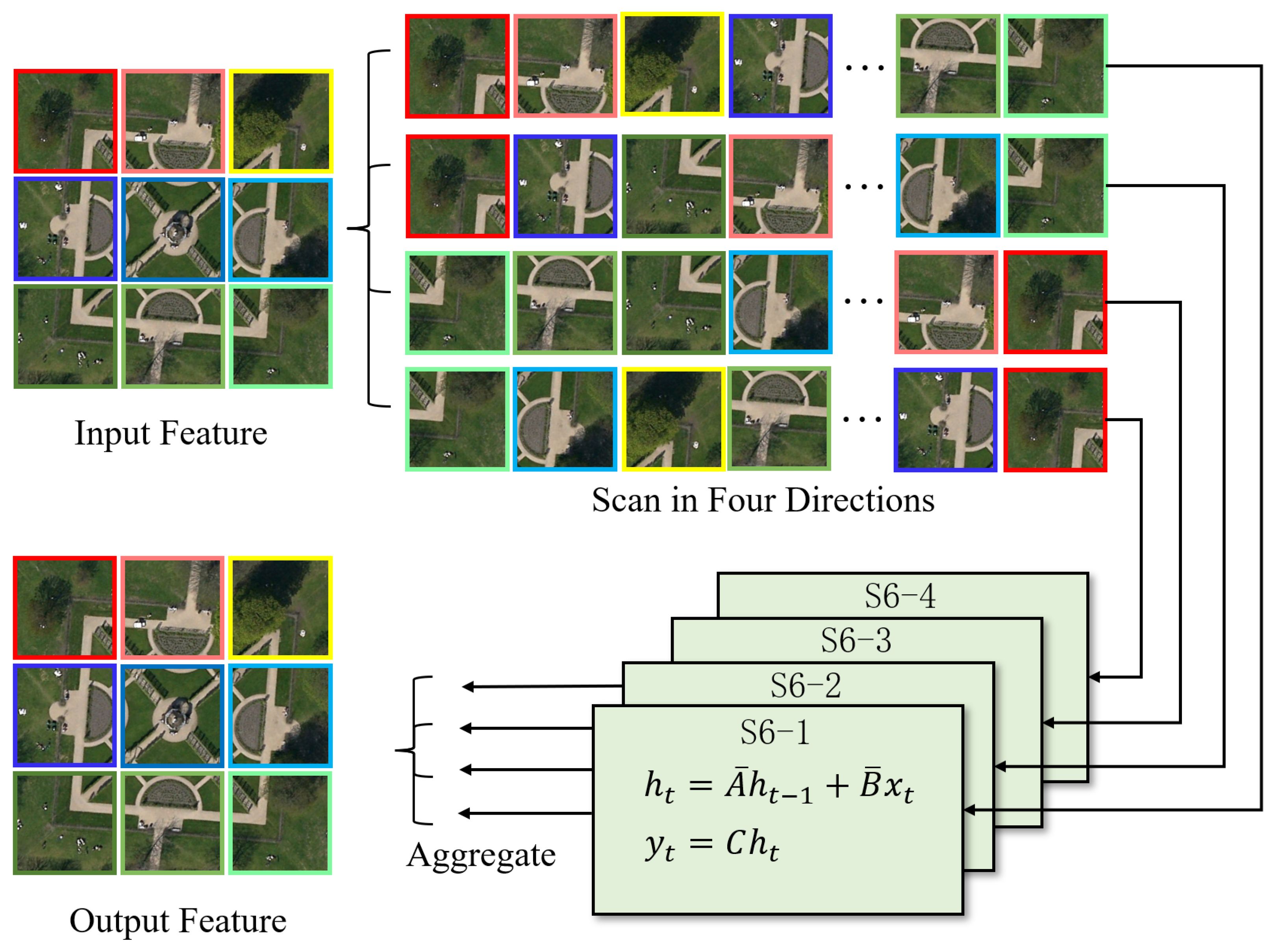
Figure 1. The comparison of receptive field among RCAN [20], SwinIR [16], and ESatSR.
Remotesensing 16 01956 g001
Figure 2. The workflow of 2D Selective Scan (SS2D). The input features are scanned in four directions, pass through four distinct S6 blocks, and are then aggregated to form the output feature.
Remotesensing 16 01956 g002
Figure 3. An overview of ESatSR’s architecture. (A) Image Feature Extraction Module, including a shallow feature extractor and several context-aware residual groups performing deep feature extraction (B) Spatial Context Interaction Module, consisting of a spatial prior information extractor, and multiple sets of spatial context mixers and spatial context separators to conduct the interaction with the deep feature extraction process. (C) Enhanced Image Reconstruction Module, utilizing the outputs of the Image Feature Extraction Module and Spatial Context Interaction Module to generate the SR result. (D) Spatial prior information extractor, including several convolutional layers to extract multi-scale spatial information. (E) Example of a spatial context mixer, mixing the image feature with spatial context. (F) Example of a spatial context separator, utilizing the image feature processed by the context-aware residual group to generate spatial context for the next mixer.
Remotesensing 16 01956 g003
Figure 4. Components of CARG. (a) The architecture of Residual VMamba Block (RVMB). The convolution is used here to enhance the capability of local feature extraction. (b) The details of the Visual State Space Block (VSSBlock), consisting of the 2D Selective Scan Module (SS2D), depth-wise convolution, and Silu activation function.
Remotesensing 16 01956 g004
Figure 5. The architecture of the Spatial Prior Information Extractor, including several convolutional layers. It extracts multi-scale spatial prior information from the LR image.
Remotesensing 16 01956 g005
Figure 6. Components of the Spatial Context Interaction Module. (a) The architecture of spatial context mixer. A cross attention is performed, where the spatial context is used as the key and value, while the image features processed by a 16 × 16 convolutional layer is used as the query. (b) The architecture of spatial context separator. A cross attention is performed, where the spatial context is used as the query, while the image features processed by the corresponding CARG and a 16 × 16 convolutional layer is used as the key and value.
Remotesensing 16 01956 g006
Figure 7. The architecture of enhanced image restoration module. The feature map is upsampled through convolution and PixelShuffle. Spatial context at three scales are fused with each other in a step-wise upsampling process. The multi-scale spatial context, low-resolution input, and deep image features are first upsampled and then input into a convolution layer to transfer from the feature dimension to the image dimension, producing the SR image.
Remotesensing 16 01956 g007
Figure 8. Qualitative comparison among ESatSR and other SR methods on the OLI2MSI(×2) dataset. For each image, the content in the yellow box has been upsampled and placed into the red box for better viewing. The methods include: (a) ECBSR, (b) EDSR, (c) RCAN, (d) SwinIR, (e) LGCNet, (f) CTN, (g) HSENet, (h) EEGAN, (i) MHAN, and (j) ESatSR.
Remotesensing 16 01956 g008
Figure 9. Qualitative comparison among ESatSR and other SR methods on the RSSCN7(×2) dataset. For each image, the content in the yellow box has been upsampled and placed into the red box for better viewing. The methods include: (a) ECBSR, (b) EDSR, (c) RCAN, (d) SwinIR, (e) LGCNet, (f) CTN, (g) HSENet, (h) EEGAN, (i) MHAN, and (j) ESatSR.
Remotesensing 16 01956 g009
Figure 10. Qualitative comparison among ESatSR and other SR methods on the OLI2MSI(×3) dataset. For each image, the content in the yellow box has been upsampled and placed into the red box for better viewing. The methods include: (a) ECBSR, (b) EDSR, (c) RCAN, (d) SwinIR, (e) LGCNet, (f) CTN, (g) HSENet, (h) EEGAN, (i) MHAN, and (j) ESatSR.
Remotesensing 16 01956 g010
Figure 11. Qualitative comparison among ESatSR and other SR methods on the RSSCN7(×3) dataset. For each image, the content in the yellow box has been upsampled and placed into the red box for better viewing. The methods include: (a) ECBSR, (b) EDSR, (c) RCAN, (d) SwinIR, (e) LGCNet, (f) CTN, (g) HSENet, (h) EEGAN, (i) MHAN, and (j) ESatSR.
Remotesensing 16 01956 g011
Figure 12. Ablation studies on different settings of ESatSR. Results are tested on OLI2MSI with scale factor 2. We use V4 in Table 4 as the default setting, and the number of corresponding components will change when the version is different.
Remotesensing 16 01956 g012
Table 1. Quantitative comparison with state-of-the-art methods on OLI2MSI (×2) and RSSCN7 (×2). The methods in the upper part are image restoration methods, while methods in the lower part are SR algorithms tailored for remote sensing images. The bold text denotes the best performance.
MethodFLOPs#ParamRSSCN7 ×2OLI2MSI ×2
PSNRSSIMLPIPSPSNRSSIMLPIPS
ECBSR [53]1.334 G0.036 M28.52430.77590.129838.13200.94530.0547
EDSR [25]398.629 G10.806 M29.84450.80530.116940.67300.97210.0346
RCAN [20]496.414 G13.559 M29.92780.80710.114640.85890.97300.0331
SwinIR [16]432.409 G11.704 M31.20120.81470.117641.93010.97790.0336
ESatSR (Ours)624.507 G23.751 M31.42430.82670.114542.11310.97840.0335
CTN [37]9.412 G0.349 M28.72040.78110.119638.30980.95010.0394
LGCNet [36]222.695 G6.042 M29.14850.78220.117438.57210.95290.0541
HSENet [40]150.332 G5.286 M29.79570.80350.115340.42280.97080.0341
EEGAN [54]214.248 G5.686 M30.57820.81050.116941.57930.97140.0338
MHAN [55]416.803 G11.203 M30.94610.81480.115641.87470.97600.0342
ESatSR (Ours)624.507 G23.751 M31.42430.82670.114542.11310.97840.0335
Table 2. Quantitative comparison with state-of-the-art methods on OLI2MSI(×3) and RSSCN7(×3). The bold text denotes the best performance.
MethodFLOPs#ParamRSSCN7 ×3OLI2MSI ×3
PSNR SSIM LPIPS PSNR SSIM LPIPS
ECBSR [53]0.593 G0.362 M26.24360.64920.181431.79600.82820.1168
EDSR [25]201.454 G12.265 M27.71120.69650.168633.02700.91190.1012
RCAN [20]223.416 G13.721 M27.75720.69810.174533.21420.91770.1004
SwinIR [16]195.343 G11.889 M29.05170.71500.169034.90300.92680.0956
ESatSR (Ours)280.720 G23.756 M29.25520.72620.162435.17440.92760.0951
CTN [37]5.835 G0.349 M26.58700.65110.176332.22430.84040.1128
LGCNet [36]98.975 G6.042 M26.66850.65260.167632.25280.84410.1170
HSENet [40]69.976 G5.470 M27.63480.69250.167233.34700.90980.1150
EEGAN [54]152.269 G5.870 M28.57820.70520.169134.57930.91140.1029
MHAN [55]191.427 G11.387 M28.94610.71090.164734.87470.91600.0913
ESatSR (Ours)280.720 G23.756 M29.25520.72620.162435.17440.92760.0951
Table 3. The effectiveness of SCIM and EIRM. SPIE, Mixer, and Separator are the components of SCIM. “Single” means EIRM only uses spatial context of the coarsest scale. “Multi” means the spatial context will be progressively upsampled. SCIM, EIRM, and SPIE are short for Spatial Context Interaction Module, Enhanced Image Reconstruction Module, and Spatial Prior Extractor.
SettingSCIMEIRMPSNRSSIM
SPIE Mixer Separator
baseline 41.95830.9771
Variant 1 Single41.96130.9772
Variant 2 Single42.04930.9778
Variant 3Single42.08550.9782
ESatSR (Ours)Multi42.11310.9784
Table 4. Different Settings of ESatSR.
SettingChannel NumberRVMB NumberCARG Number
V19011
V212022
V315044
V418066
V521088
V62401010
Disclaimer/Publisher’s Note: The statements, opinions and data contained in all publications are solely those of the individual author(s) and contributor(s) and not of MDPI and/or the editor(s). MDPI and/or the editor(s) disclaim responsibility for any injury to people or property resulting from any ideas, methods, instructions or products referred to in the content.