Figure 1.
Illustration of DSConv and CBAM. The label “Conv” means the standard convolution, and “Conv1×1” indicates the convolution with the 1×1 kernel. “H”, “W”, and “C” denote the height, width, and channel. “MaxPool” and “AvgPool” denote the max pooling and average pooling, respectively.
Figure 1.
Illustration of DSConv and CBAM. The label “Conv” means the standard convolution, and “Conv1×1” indicates the convolution with the 1×1 kernel. “H”, “W”, and “C” denote the height, width, and channel. “MaxPool” and “AvgPool” denote the max pooling and average pooling, respectively.
Figure 2.
Illustration of the proposed LRSDN model.
Figure 2.
Illustration of the proposed LRSDN model.
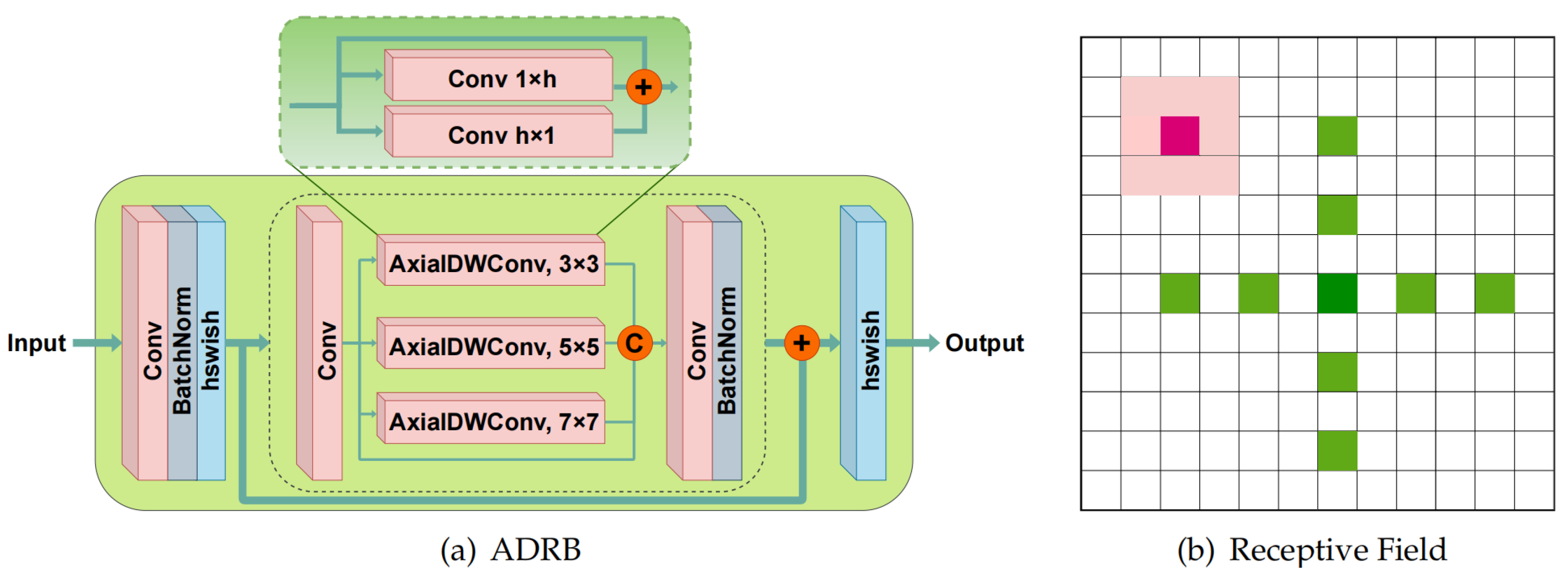
Figure 3.
Illustration of the proposed ADRB and the receptive field of AxialDWConv. In (a), “C” means the concatenation operation, and “+” represents elementwise addition. The dashed box below depicts the structure of the ADWConvBlock, while the smaller dashed box above details an AxialDWConv operator. (b) compares the receptive fields of the typical 3×3 convolution and the 5×5 AxialDWConv (dilation = 2), marked in red and green, respectively. AxialDWConv offers a much larger receptive field than the standard convolution with the same computational parameters.
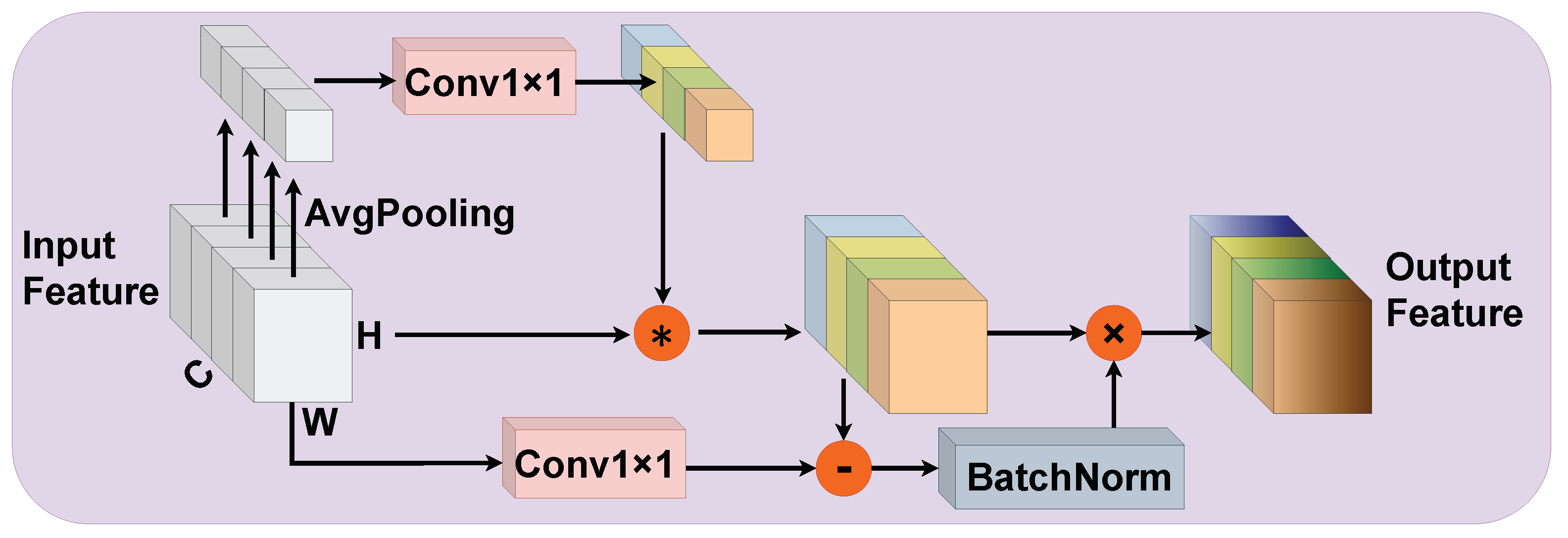
Figure 4.
Illustration of the proposed HAB. “×” and “*” represent elementwise and channelwise multiplication, respectively. “-” denotes elementwise subtraction.
Figure 4.
Illustration of the proposed HAB. “×” and “*” represent elementwise and channelwise multiplication, respectively. “-” denotes elementwise subtraction.
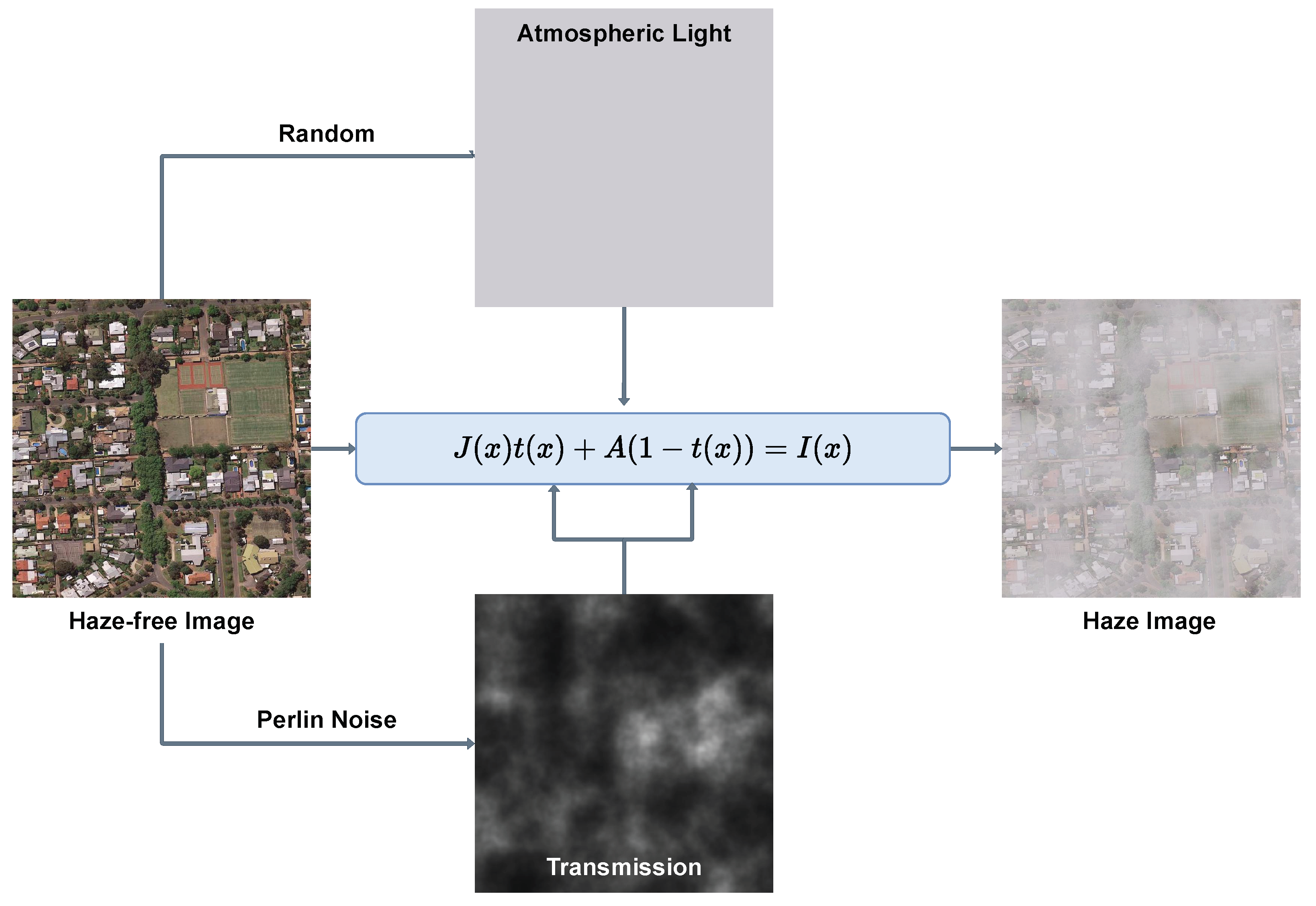
Figure 5.
Illustration of the proposed haze-image-simulation method based on Perlin noise and the atmospheric scattering model.
Figure 5.
Illustration of the proposed haze-image-simulation method based on Perlin noise and the atmospheric scattering model.
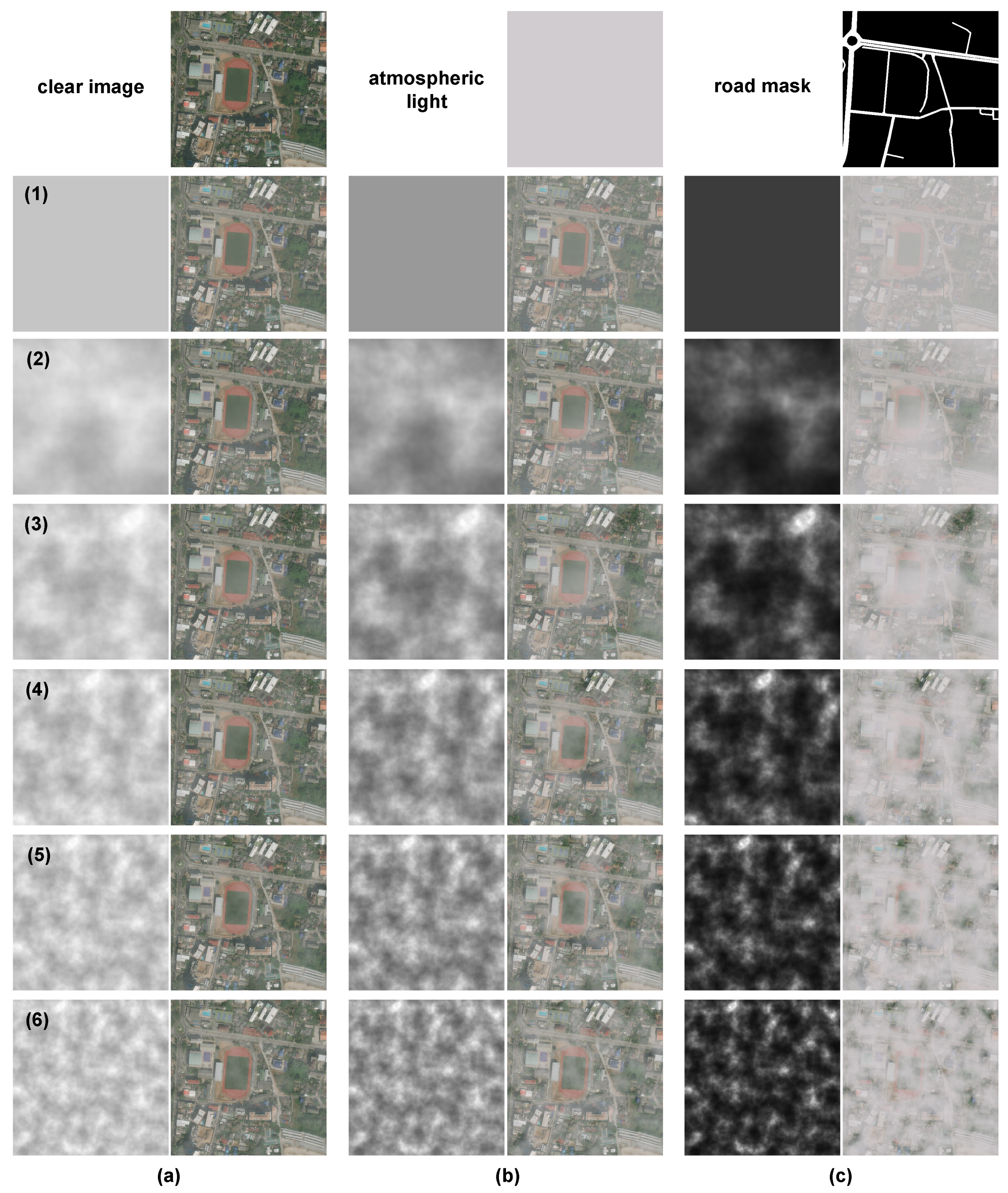
Figure 6.
The synthesized samples in the proposed RSHD. In the top row, the haze-free remote sensing image, randomly generated atmospheric light, and the corresponding road mask are displayed from left to right. Images in each row are synthesized hazy samples with varying uniformity in haze distribution. Columns (a–c) represent samples with varying haze concentrations, namely thin haze, moderate haze, and dense haze, respectively. In each pair of images, the grayscale image on the left represents the transmission, while the corresponding synthetic haze image is depicted on the right.
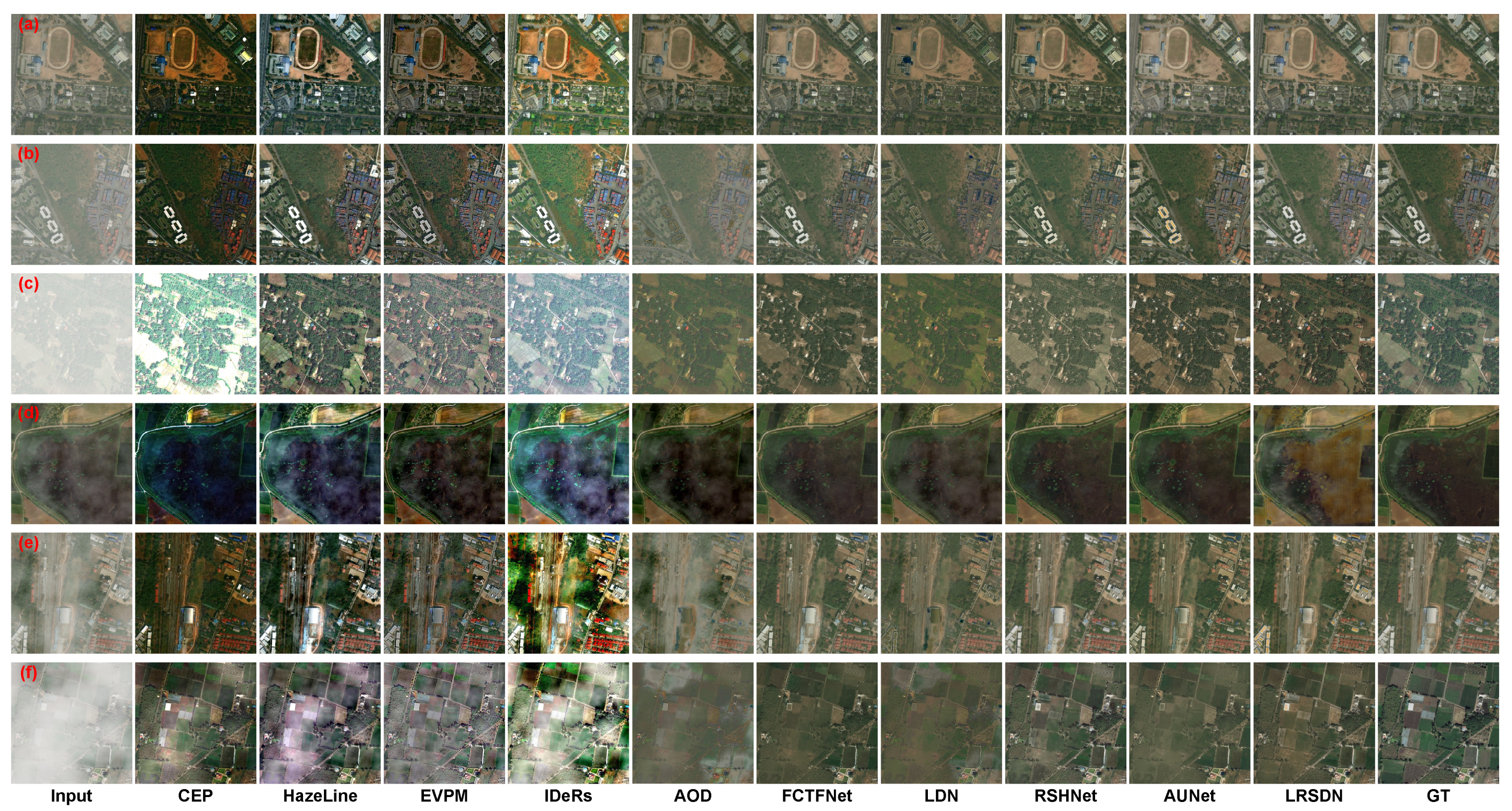
Figure 7.
Visual comparisons of dehazed results by different methods on the proposed RSHD. “GT” indicates ground truth. (a–f) are samples from the RSHD-HT, RSHD-HM, RSHD-HD, RSHD-IHT, RSHD-IHM, and RSHD-IHD test sets, respectively.
Figure 7.
Visual comparisons of dehazed results by different methods on the proposed RSHD. “GT” indicates ground truth. (a–f) are samples from the RSHD-HT, RSHD-HM, RSHD-HD, RSHD-IHT, RSHD-IHM, and RSHD-IHD test sets, respectively.
Figure 8.
Visual comparisons of dehazed results by different methods on Haze1K dataset. (g–i) are samples from the thin, moderate, and thick haze subsets of the Haze1K test set, respectively.
Figure 8.
Visual comparisons of dehazed results by different methods on Haze1K dataset. (g–i) are samples from the thin, moderate, and thick haze subsets of the Haze1K test set, respectively.
Figure 9.
Visual comparisons of dehazed results by different methods on the RICE dataset.
Figure 9.
Visual comparisons of dehazed results by different methods on the RICE dataset.
Figure 10.
Visual comparisons of dehazed results by different methods on RSID dataset.
Figure 10.
Visual comparisons of dehazed results by different methods on RSID dataset.
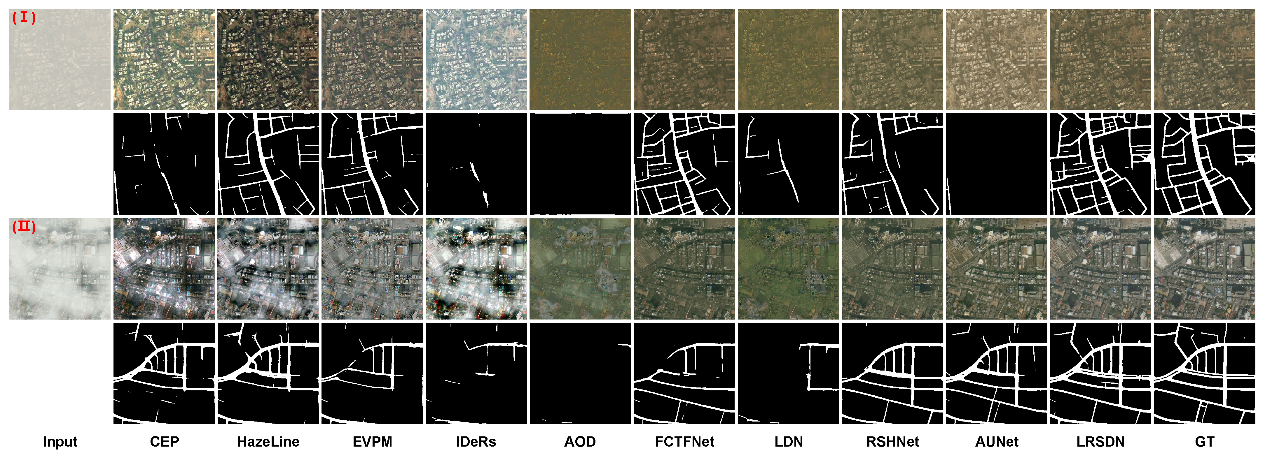
Figure 11.
Visual comparisons of dehazed results and corresponding road-extraction results by different methods on the RSHD. The sample (I) is from the homogeneous and dense haze subset RSHD-HD, and the sample (II) is from the inhomogeneous and dense haze subset RSHD-IHD.
Figure 11.
Visual comparisons of dehazed results and corresponding road-extraction results by different methods on the RSHD. The sample (I) is from the homogeneous and dense haze subset RSHD-HD, and the sample (II) is from the inhomogeneous and dense haze subset RSHD-IHD.
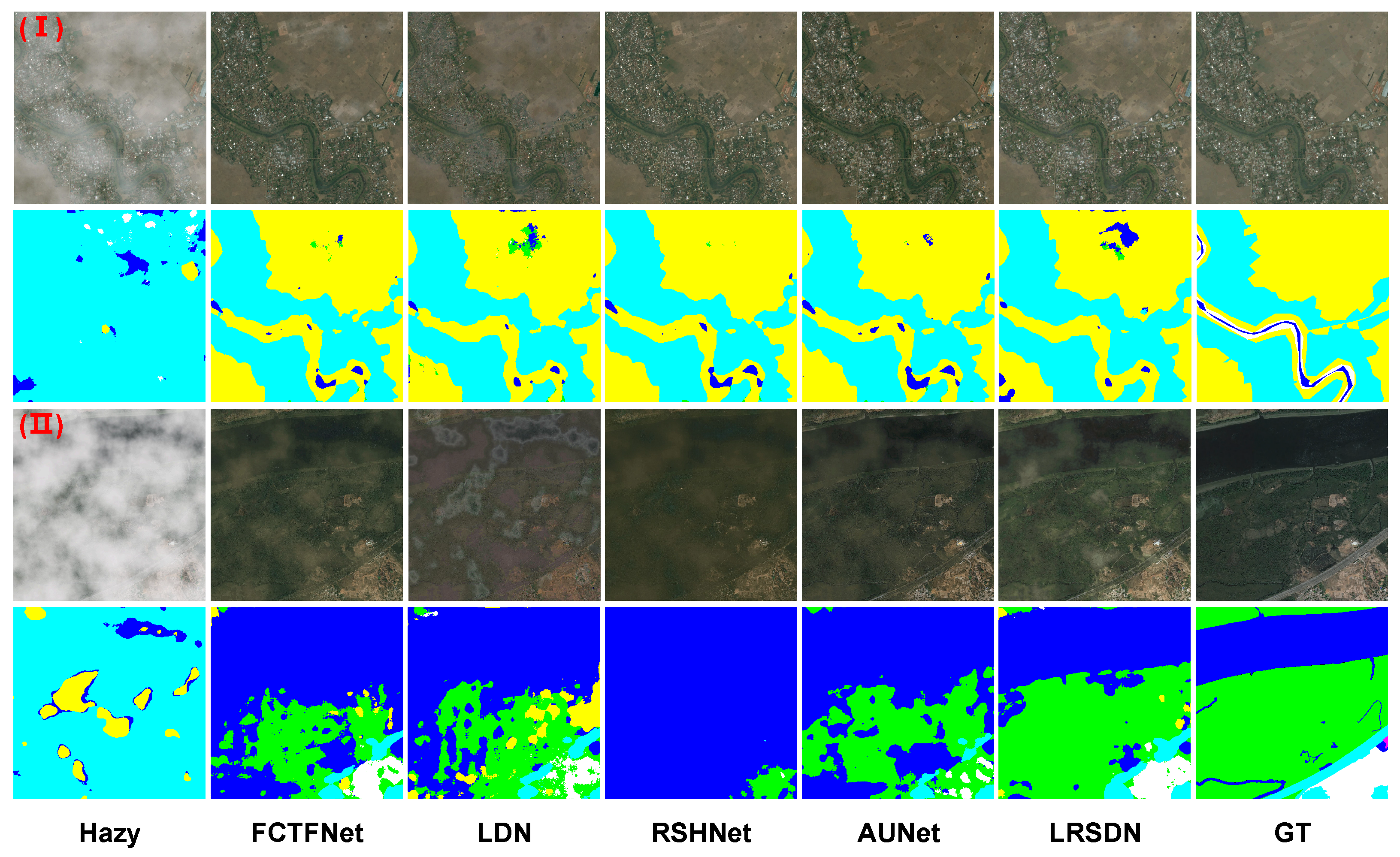
Figure 12.
Visual comparisons of dehazed results and corresponding land cover-classification results by different deep learning-based methods. “GT” means the haze-free images and the labeled land cover masks.
Figure 12.
Visual comparisons of dehazed results and corresponding land cover-classification results by different deep learning-based methods. “GT” means the haze-free images and the labeled land cover masks.
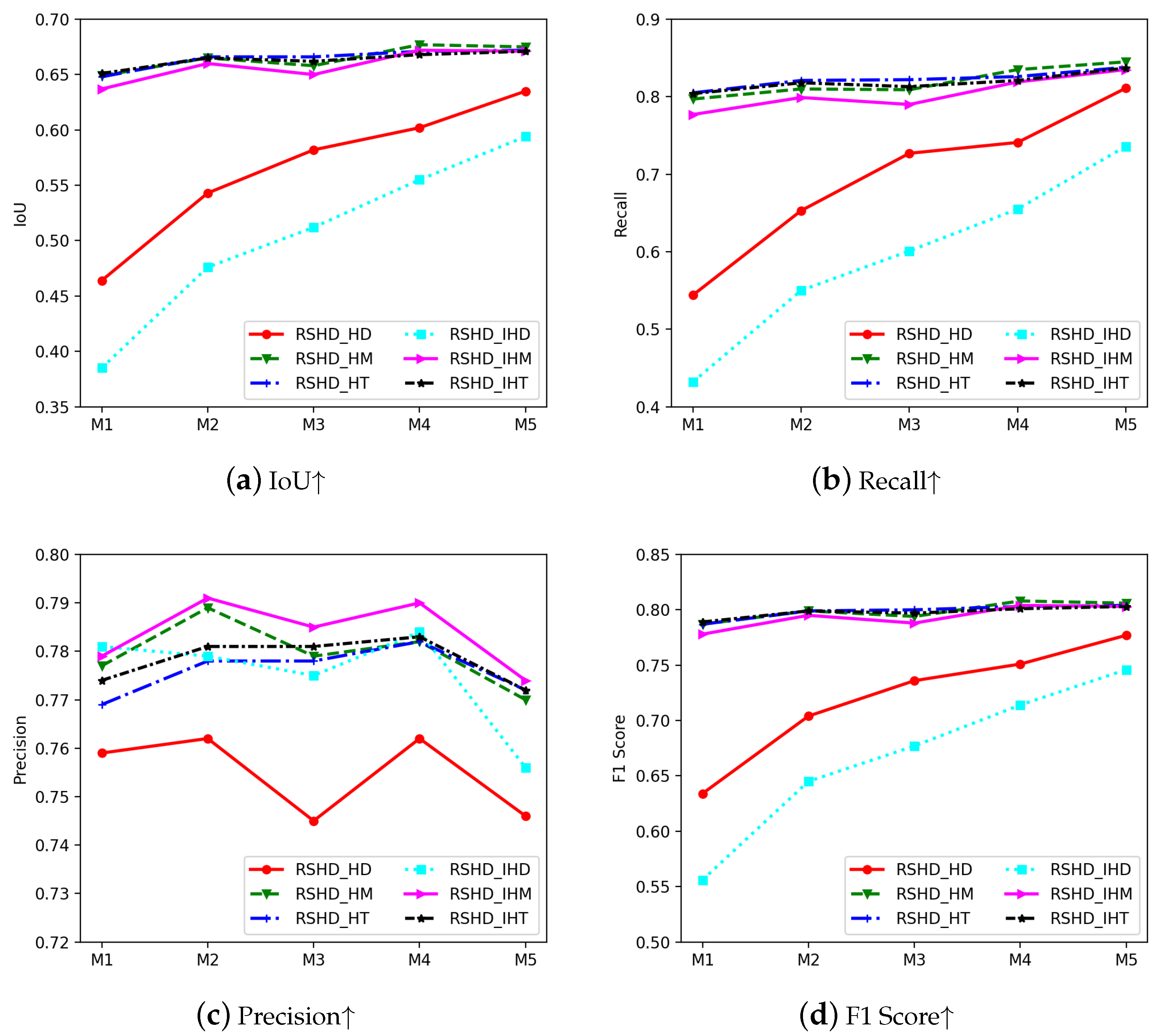
Figure 13.
Full-reference assessment comparisons of all variant models dehazing on 6 test sets of RSHD.
Figure 13.
Full-reference assessment comparisons of all variant models dehazing on 6 test sets of RSHD.
Figure 14.
Quantitative results of road extraction on dehazed images by each variant model.
Figure 14.
Quantitative results of road extraction on dehazed images by each variant model.
Figure 15.
Visualization of the feature maps obtained by each BasicBlock of the LRSDN model. The caption of each subfigure identifies its derivation. The number indicates the order of the current BasicBlock: “A” and “B” stand for “after” and “before” (relative to the HAB). For example, “3-B” indicates that the feature is from the intermediate output before the the HAB of the 3rd BasicBlock.
Figure 16.
Failure cases of the proposed LRSDN. The top row shows hazy samples, and the bottom row shows the corresponding dehazed results by the LRSDN.
Figure 16.
Failure cases of the proposed LRSDN. The top row shows hazy samples, and the bottom row shows the corresponding dehazed results by the LRSDN.
Table 1.
The overview of existing datasets, where “RSHD” means the datasets constructed in this paper.
Table 1.
The overview of existing datasets, where “RSHD” means the datasets constructed in this paper.
| Name | Test Size | Training Size | Spatial Resolution | Pixel
Resolution | Distribution Diversity | Density Diversity | High-Level Task |
|---|
| Hazelk-thin [47] | 45 | 320 | 0.8 m | 512 × 512 | ⨂ | √ | × |
| Haze1k-moderate [47] | 45 | 320 |
| Haze1k-thick [47] | 45 | 320 |
| RICE [48] | 8 | 420 | 15m | 512 × 512 | ⨂ | × | × |
| RSID [31] | 100 | 900 | # | 256 × 256 | ⨂ | × | × |
| DHID [49] | 500 | 14,490 | 0.13 m | 512 × 512 | ⨂ | × | × |
| LHID [49] | 1000 | 30,517 | 0.2–153 m | 512 × 512 | × | × | × |
| RSHD-HT | 510 | 42,240 | 0.3/0.05 m | 1024 × 1024 | √ | √ | √ |
| RSHD-HM | 510 |
| RSHD-HD | 510 |
| RSHD-IHT | 510 |
| RSHD-IHM | 510 |
| RSHD-IHD | 510 |
Table 2.
Quantitative comparisons of different algorithms’ dehazing on the RSHD. The abbreviations “HD”, “HM”, “HT”, “IHD”, “IHM”, and “IHT” in the dataset name stand for the six subsets of the RSHD (referring to
Table 1), respectively. ↑ indicates better performance with a higher value, while ↓ means the opposite case, and text in bold indicates the best results (all subsequent tables follow this convention).
| Dataset | Metrics | CEP[9] | HazeLine[11] | EVPM[12] | IDeRs[21] | AOD [13] | FCTFNet[15] | LDN[14] | RSHNet[35] | AUNet[50] | LRSDN |
|---|
| HD | LPIPS↓ | 0.450 | 0.378 | 0.407 | 0.469 | 0.372 | 0.331 | 0.348 | 0.393 | 0.346 | 0.301 |
| PSNR↑ | 16.346 | 19.609 | 16.827 | 10.040 | 21.298 | 23.985 | 21.544 | 23.117 | 22.629 | 26.871 |
| SSIM↑ | 0.716 | 0.732 | 0.704 | 0.626 | 0.786 | 0.827 | 0.806 | 0.822 | 0.830 | 0.845 |
| FSIM↑ | 0.847 | 0.852 | 0.860 | 0.885 | 0.807 | 0.922 | 0.876 | 0.949 | 0.949 | 0.966 |
| HM | LPIPS↓ | 0.386 | 0.283 | 0.284 | 0.399 | 0.216 | 0.165 | 0.185 | 0.187 | 0.177 | 0.172 |
| PSNR↑ | 14.582 | 19.826 | 19.628 | 16.458 | 19.758 | 28.284 | 23.940 | 28.736 | 28.737 | 29.856 |
| SSIM↑ | 0.696 | 0.769 | 0.737 | 0.608 | 0.848 | 0.898 | 0.879 | 0.896 | 0.901 | 0.903 |
| FSIM↑ | 0.818 | 0.850 | 0.890 | 0.790 | 0.892 | 0.970 | 0.932 | 0.980 | 0.986 | 0.986 |
| HT | LPIPS↓ | 0.375 | 0.276 | 0.244 | 0.359 | 0.141 | 0.126 | 0.133 | 0.135 | 0.153 | 0.130 |
| PSNR↑ | 13.758 | 18.576 | 18.079 | 18.104 | 23.116 | 31.161 | 26.537 | 29.693 | 29.242 | 31.748 |
| SSIM↑ | 0.675 | 0.744 | 0.761 | 0.654 | 0.894 | 0.913 | 0.898 | 0.904 | 0.903 | 0.913 |
| FSIM↑ | 0.825 | 0.836 | 0.924 | 0.820 | 0.963 | 0.988 | 0.956 | 0.985 | 0.987 | 0.989 |
| IHD | LPIPS↓ | 0.414 | 0.488 | 0.489 | 0.504 | 0.452 | 0.377 | 0.408 | 0.434 | 0.371 | 0.345 |
| PSNR↑ | 16.680 | 12.486 | 15.435 | 9.914 | 17.878 | 22.930 | 20.093 | 22.529 | 23.047 | 25.544 |
| SSIM↑ | 0.744 | 0.686 | 0.669 | 0.608 | 0.736 | 0.798 | 0.771 | 0.782 | 0.806 | 0.817 |
| FSIM↑ | 0.814 | 0.730 | 0.744 | 0.720 | 0.759 | 0.890 | 0.821 | 0.882 | 0.912 | 0.929 |
| IHM | LPIPS↓ | 0.356 | 0.331 | 0.310 | 0.382 | 0.254 | 0.173 | 0.196 | 0.203 | 0.190 | 0.182 |
| PSNR↑ | 15.391 | 16.903 | 19.032 | 15.790 | 18.645 | 27.851 | 23.397 | 27.887 | 25.407 | 29.110 |
| SSIM↑ | 0.731 | 0.743 | 0.743 | 0.643 | 0.831 | 0.895 | 0.874 | 0.891 | 0.890 | 0.899 |
| FSIM↑ | 0.838 | 0.792 | 0.857 | 0.775 | 0.846 | 0.966 | 0.921 | 0.970 | 0.967 | 0.976 |
| IHT | LPIPS↓ | 0.367 | 0.307 | 0.249 | 0.353 | 0.160 | 0.129 | 0.140 | 0.141 | 0.160 | 0.133 |
| PSNR↑ | 13.977 | 17.190 | 18.042 | 17.976 | 22.142 | 29.950 | 25.775 | 28.630 | 28.264 | 31.317 |
| SSIM↑ | 0.684 | 0.711 | 0.765 | 0.665 | 0.887 | 0.911 | 0.896 | 0.903 | 0.900 | 0.912 |
| FSIM↑ | 0.831 | 0.812 | 0.916 | 0.822 | 0.945 | 0.983 | 0.949 | 0.981 | 0.979 | 0.987 |
Table 3.
Quantitative comparisons of different algorithms’ dehazing on the Haze1K dataset.
Table 3.
Quantitative comparisons of different algorithms’ dehazing on the Haze1K dataset.
| Dataset | Metrics | CEP[9] | HazeLine[11] | EVPM [12] | IDeRs[21] | AOD[13] | FCTFNet[15] | LDN[14] | RSHNet[35] | AUNet[50] | LRSDN |
|---|
| Thick | LPIPS↓ | 0.222 | 0.186 | 0.210 | 0.311 | 0.238 | 0.207 | 0.232 | 0.220 | 0.190 | 0.157 |
| PSNR↑ | 15.089 | 16.365 | 16.647 | 11.754 | 16.521 | 19.192 | 16.506 | 20.258 | 19.909 | 21.897 |
| SSIM↑ | 0.759 | 0.790 | 0.787 | 0.702 | 0.774 | 0.814 | 0.777 | 0.835 | 0.837 | 0.847 |
| FSIM↑ | 0.889 | 0.914 | 0.901 | 0.872 | 0.864 | 0.937 | 0.862 | 0.941 | 0.948 | 0.959 |
| Moderate | LPIPS↓ | 0.274 | 0.198 | 0.104 | 0.320 | 0.175 | 0.081 | 0.116 | 0.061 | 0.104 | 0.088 |
| PSNR↑ | 13.083 | 15.454 | 20.656 | 14.763 | 20.078 | 23.582 | 20.970 | 24.880 | 24.327 | 25.241 |
| SSIM↑ | 0.746 | 0.798 | 0.918 | 0.785 | 0.906 | 0.937 | 0.921 | 0.941 | 0.929 | 0.934 |
| FSIM↑ | 0.854 | 0.895 | 0.942 | 0.899 | 0.917 | 0.969 | 0.936 | 0.966 | 0.956 | 0.970 |
| Thin | LPIPS↓ | 0.287 | 0.183 | 0.088 | 0.279 | 0.098 | 0.091 | 0.095 | 0.083 | 0.071 | 0.070 |
| PSNR↑ | 12.194 | 13.921 | 20.426 | 15.048 | 18.671 | 21.532 | 18.648 | 22.377 | 23.017 | 23.673 |
| SSIM↑ | 0.701 | 0.760 | 0.891 | 0.772 | 0.870 | 0.898 | 0.873 | 0.903 | 0.906 | 0.913 |
| FSIM↑ | 0.834 | 0.892 | 0.962 | 0.911 | 0.943 | 0.965 | 0.947 | 0.967 | 0.976 | 0.978 |
Table 4.
Quantitative comparisons of different algorithms’ dehazing on the RICE dataset.
Table 4.
Quantitative comparisons of different algorithms’ dehazing on the RICE dataset.
| Metrics | CEP [9] | HazeLine [11] | EVPM [12] | IDeRs [21] | AOD [13] | FCTFNet [15] | LDN [14] | RSHNet [35] | AUNet [50] | LRSDN |
|---|
| LPIPS↓ | 0.341 | 0.288 | 0.293 | 0.363 | 0.274 | 0.072 | 0.183 | 0.106 | 0.075 | 0.077 |
| PSNR↑ | 14.234 | 17.058 | 15.217 | 15.750 | 20.784 | 29.091 | 23.108 | 23.453 | 28.704 | 31.662 |
| SSIM↑ | 0.713 | 0.723 | 0.742 | 0.611 | 0.834 | 0.949 | 0.873 | 0.919 | 0.946 | 0.953 |
| FSIM↑ | 0.800 | 0.781 | 0.865 | 0.746 | 0.856 | 0.980 | 0.887 | 0.961 | 0.980 | 0.983 |
Table 5.
Quantitative comparisons of different algorithms’ dehazing on RSID dataset.
Table 5.
Quantitative comparisons of different algorithms’ dehazing on RSID dataset.
| Metrics | CEP [9] | HazeLine [11] | EVPM [12] | IDeRs [21] | AOD [13] | FCTFNet [15] | LDN [14] | RSHNet [35] | AUNet [50] | LRSDN |
|---|
| LPIPS↓ | 0.277 | 0.191 | 0.202 | 0.277 | 0.144 | 0.093 | 0.125 | 0.127 | 0.054 | 0.076 |
| PSNR↑ | 13.091 | 16.498 | 16.418 | 14.254 | 19.052 | 22.469 | 19.026 | 20.640 | 25.457 | 24.878 |
| SSIM↑ | 0.736 | 0.848 | 0.779 | 0.713 | 0.901 | 0.939 | 0.912 | 0.912 | 0.957 | 0.942 |
| FSIM↑ | 0.796 | 0.873 | 0.826 | 0.777 | 0.911 | 0.944 | 0.925 | 0.929 | 0.962 | 0.947 |
Table 6.
The average scores of the quantitative evaluation of the road-extraction results by different methods on the RSHD.
Table 6.
The average scores of the quantitative evaluation of the road-extraction results by different methods on the RSHD.
| Metrics | CEP [9] | HazeLine [11] | EVPM [12] | IDeRs [21] | AOD [13] | FCTFNet [15] | LDN [14] | RSHNet [35] | AUNet [50] | LRSDN |
|---|
| Recall↑ | 0.546 | 0.668 | 0.681 | 0.397 | 0.508 | 0.709 | 0.634 | 0.726 | 0.775 | 0.783 |
| Precision↑ | 0.718 | 0.742 | 0.733 | 0.696 | 0.741 | 0.780 | 0.789 | 0.771 | 0.760 | 0.780 |
| IoU↑ | 0.450 | 0.541 | 0.544 | 0.342 | 0.429 | 0.589 | 0.528 | 0.594 | 0.623 | 0.641 |
| F1↑ | 0.619 | 0.700 | 0.699 | 0.497 | 0.570 | 0.736 | 0.674 | 0.741 | 0.766 | 0.780 |
Table 7.
The average scores of the quantitative evaluation of the land cover classification results by different methods.
Table 7.
The average scores of the quantitative evaluation of the land cover classification results by different methods.
| Metrics | Hazy | CEP [9] | EVPM [12] | IDeRs [21] | AOD [13] | FCTFNet [15] | LDN [14] | RSHNet [35] | AUNet [50] | LRSDN |
|---|
| IoU↑ | 0.161 | 0.483 | 0.381 | 0.286 | 0.476 | 0.581 | 0.591 | 0.527 | 0.496 | 0.593 |
| F1↑ | 0.229 | 0.616 | 0.479 | 0.403 | 0.596 | 0.699 | 0.704 | 0.639 | 0.609 | 0.709 |
| Recall↑ | 0.201 | 0.576 | 0.458 | 0.331 | 0.553 | 0.655 | 0.664 | 0.602 | 0.572 | 0.658 |
| Precision↑ | 0.293 | 0.675 | 0.509 | 0.595 | 0.685 | 0.774 | 0.782 | 0.698 | 0.679 | 0.805 |
Table 8.
Computational complexity and run time of several state-of-the-art algorithms.
Table 8.
Computational complexity and run time of several state-of-the-art algorithms.
| Methods | Params (M) | MACs (G) | Run Time (ms) | Methods | Run Time (ms) |
|---|
| RSHNet [35] | 1.136 | 9.850 | 14.130 | DCP [8] | 306.251 |
| AOD [13] | 0.002 | 0.107 | 0.850 | CEP [9] | 9.182 |
| GCANet [16] | 0.670 | 17.507 | 7.860 | HazeLine [11] | 1607.788 |
| GDN [17] | 0.911 | 19.969 | 17.170 | EVPM [12] | 47.704 |
| FCTFNet [15] | 0.156 | 9.357 | 8.416 | IDeRs [21] | 304.158 |
| LDN [14] | 0.029 | 1.836 | 1.160 | SMIDCP [22] | 114.872 |
| AUNet [50] | 7.417 | 48.312 | 30.230 | CAP [10] | 48.132 |
| LRSDN (ours) | 0.087 | 5.209 | 7.664 | | |
Table 9.
Computational complexity and run time of several variants of LRSDN for ablation study. The label K represents the number of Basicblocks in the model. ADRB and HAB indicate whether the BasicBlock contains the corresponding component or not. SCA and PA denote the simplified channel attention and pixel attention structures in the HAB, respectively. The BasicBlock of model M1 contains only the standard ResBlock [
19] as the baseline. The model M4 is the proposed LRSDN.
| Model | ADRB | HAB | K | Params (M) | MACs (G) | Run Time (ms) |
|---|
| M1 | × | × | 5 | 0.074 | 4.716 | 2.111 |
| M2 |
√
| × | 5 | 0.080 | 5.055 | 6.327 |
| M3 |
√
| SCA | 5 | 0.085 | 5.064 | 7.550 |
| M4 |
√
| SCA+PA | 5 | 0.087 | 5.209 | 7.664 |
| M5 |
√
| SCA+PA | 10 | 0.368 | 22.109 | 16.307 |


