Analysis of Lake Area Dynamics and Driving Forces in the Jianghan Plain Based on GEE and SEM for the Period 1990 to 2020

Abstract

The lakes of Jianghan Plain, as an important component of the water bodies in the middle and lower reaches of the Yangtze River plain, have made significant contributions to maintaining the ecological health and promoting the sustainable development of the Jianghan Plain. However, there is a relatively limited understanding regarding the trends of lake area change for different types of lakes and their dominant factors over the past three decades in the Jianghan Plain. Based on the Google Earth Engine (GEE) platform, combined with the water body index method, the changes in area of three different types of lakes (area > 1 km²) in the Jianghan Lake Group from 1990 to 2020 were extracted and analyzed. Additionally, the Partial least squares structural equation model (PLS-SEM) was utilized to analyze the driving factors affecting the changes in water body area of these lakes. The results show that from 1990 to 2020, the area of the lakes of the wet season and level season exhibited a decreasing trend, decreasing by 893.1 km² and 77.9 km², respectively. However, the area of dry season lakes increased by 59.27 km². The areas of all three types of lakes reached their minimum values in 2006. According to the PLS-SEM results, the continuous changes in the lakes’ area are mainly controlled by environmental factors overall. Furthermore, human factors mainly influence the mutation of the lakes’ area. This study achieved precise extraction of water body areas and accurate analysis of driving factors, providing a basis for a comprehensive understanding of the dynamic changes in the lakes of Jianghan Plain, which is beneficial for the rational utilization and protection of water resources.

1. Introduction

Water resources play a crucial role in human life and in promoting social, economic, and ecological sustainable development [1]. Lakes, rivers, and other surface water bodies, as important components of water resources, provide a range of ecological services such as climate regulation and material cycling [2,3]. In recent decades, China has experienced rapid urbanization. Due to climate change and human activities, surface water bodies have undergone significant alterations, thereby affecting surface temperature, soil moisture, biodiversity, ecosystem functions, and the socioeconomic development of human society [4,5,6,7]. Therefore, conducting dynamic monitoring of surface water bodies is of paramount importance for maintaining ecosystem health and fostering sustainable socioeconomic development.

Remote sensing imagery plays a vital role in monitoring the spatiotemporal changes of surface water bodies. For instance, Moderate Resolution Imaging Spectroradiometer (MODIS) [8,9,10,11,12], Land Remote Sensing Satellite (Landsat) [13,14,15,16], and Sentinel imagery [17,18,19] have played significant roles in this context. However, in the processing of long time series remote sensing imagery, the large volume of data and high computational complexity make it difficult to handle a large number of remote sensing images, thus making it challenging to achieve spatiotemporal monitoring of water bodies over a long time series [20]. In recent years, with the establishment and development of Google Earth Engine (GEE), its powerful cloud computing and massive multi-source data have greatly propelled the development of large-scale and long-term spatial research [21,22,23,24]. The GEE cloud platform can be used to access remote sensing images from databases, reducing the need for a large number of images. Recently, many scholars have successfully extracted a large amount of surface water using the GEE platform [25,26,27,28]. During the threshold iteration process of the water index method, it is possible to simultaneously observe the effectiveness of water extraction images and validate the accuracy of results. In theory, the GEE platform can be utilized to explore the optimal water extraction methods for any image area, significantly improving efficiency. Furthermore, the vast remote sensing data available on the GEE platform can be used to analyze the driving forces behind changes in water area within a watershed [28].

The water index method is widely applied in the extraction of surface water bodies [29,30,31,32]. Common water indices include the normalized difference water index (NDWI) [33], modified normalized difference water index (MNDWI) [34], automated water extraction index (AWEI) [35], and others. But it is challenging to distinguish water bodies from non-water bodies using a single threshold due to the spatiotemporal heterogeneity of water spectral characteristics [29]. Another commonly used method involves developing classification models using a series of predictor variables, including original spectral bands and water indices, to extract water bodies. Common classification models include support vector machines (SVMs), maximum likelihood (ML), random forest (RF), and others [36,37,38,39]. However, for these classification models, the accuracy is influenced by the training samples, predictor variables, and model parameters. Additionally, these classification models also require more time for generating classification results. However, for large-scale mapping of open-surface water bodies by using GEE, there is a need to develop a simple and high-precision extraction method for water. Recently, Zou et al. [26] established water detection rules for long-term open-surface water bodies over the United States, by using the Modified Normalized Difference Water Index (MNDWI), a Normalized Difference Vegetation Index (NDVI) [40], and an Enhanced Vegetation Index (EVI) [41]. If pixels meet the following criteria: EVI < 0.1 and (MNDWI > NDVI or MNDWI > EVI), they are classified as water bodies [26]. In contrast to classification models that require a large number of training samples and computational resources, this method achieves water body extraction by combining water body indices. It has the advantages of low data requirements and ease of implementation [26]. Zhou et al. [42] used Zou’s water detection rules on the GEE platform. They applied them to monitor lake dynamics in the Mongolian Plateau. These rules ensure high precision and rapid efficiency [42]. Therefore, it is suitable for large-scale applications in GEE.

Compare structural equation modeling (SEM) to traditional multivariate statistical methods such as multiple regression, principal component analysis, and cluster analysis. Use SEM to simultaneously study the correlations between structures composed of numerous variables, and it can clearly demonstrate the strength of each association [43]. Partial Least Squares Structural Equation Modeling (PLS-SEM), as one of the SEM models, relaxes assumptions about data normality and does not impose constraints on the number of observed variables [44]. And traditional statistical techniques may not effectively analyze these latent variables. However, SEM can efficiently analyze both these latent variables and their indicators [45]. The main advantages of PLS-SEM include its ability to simultaneously handle multiple sets of dependent variables, accommodate measurement errors in both independent and dependent variables, estimate the structure of factors and their relationships, provide greater flexibility to measurement models, and estimate the overall model [46]. Currently, PLS-SEM has garnered increasing attention in other fields and is widely applied in areas such as geography, economics, and natural environment studies [47,48,49,50].

So far, despite the increased attention of many researchers on the changes in water bodies in the middle and lower reaches of the Yangtze River, they have conducted in-depth studies on the changes in water bodies in the Yangtze River basin. These studies have revealed the impact of factors such as climate change and human activities on water body changes, providing important scientific evidence for water resource management and ecological conservation [51,52,53,54]. Chang et al. [50] analyzed the spatial patterns of water bodies in the Jianghan Plain from 2000 to 2020. Their findings indicated a trend of fragmentation, reduced shape complexity, and diminished connectivity in water bodies. These changes were primarily driven by human activity. Wei et al. [52] quantitatively analyzed the area changes of Hong Lake and Chang Lake from 2000 to 2018. They found that Hong Lake fluctuated due to groundwater and human factors, while Chang Lake remained stable under water control measures. Feng et al. [53] analyzed the spatiotemporal evolution of lakes and their relationship with human activities from 1984 to 2014. The results indicated that the return of farmland to lakes had a positive impact on lake conservation and restoration, while rapid agricultural development led to excessive exploitation of lake resources. Song et al. [54] used XGBoost and ICESat-2 imagery to analyze changes in water levels and storage volumes of Chinese lakes. The results indicate that the Jianghan Plain region contributes significantly to variations in lake storage volume in China, primarily due to the changes in lake water levels in that area. However, there is a relatively limited amount of long-term time series research on the dynamic changes of lakes area in the Jianghan Plain. Additionally, further research is needed to investigate the effects of different influencing factors on the dynamic changes of a lakes’ area during different periods in the Jianghan Plain.

Therefore, our specific research objectives are (1) to extract and analyze the annual trends of the lakes’ area and their dynamic changes during different periods. (2) To investigate the relationship between changes in lake water area during different periods and climates, as well as climate factors, utilizing meteorological data and statistical yearbook data. (3) Use the PLS-SEM model to identify the primary influencing factors of lake water area changes during different periods in the Jianghan Plain. The innovation of this study lies in conducting a long-term time-series analysis of the changes in lake water area and their driving factors during different periods in the Jianghan Plain, by integrating GEE and PLS-SEM. Additionally, at the watershed scale, this study identifies the primary drivers of changes in the lakes’ area during the wet periods, level periods, and dry periods. This study contributes to a better understanding of the dynamic changes in lakes during different periods in the Jianghan Plain. It aids in maintaining regional ecological balance and improving the rational utilization and management of water resources.

2. Materials and Methods

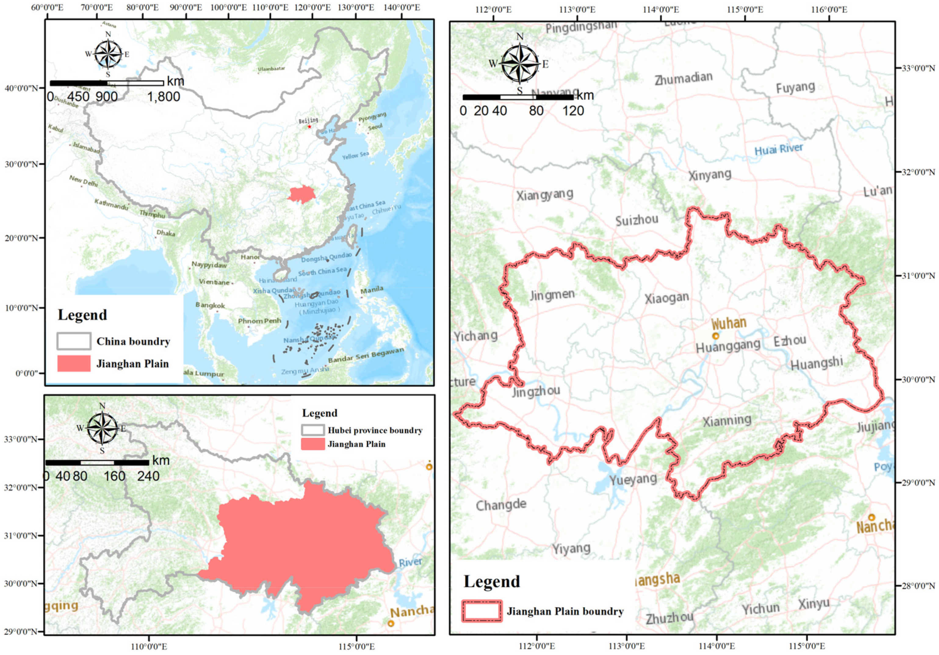
2.1. Study Area and Experimental Design

The Jianghan Plain, located in the central-southern part of Hubei province, is formed by the alluvial deposits of the Yangtze River and the Han River. The Jianghan Plain has a subtropical monsoon climate, with an annual average temperature ranging from 15.9 to 16.5 degrees Celsius. The annual average precipitation falls between 1100 and 1400 mm, with the majority occurring during the summer months. Considering the completeness of administrative divisions, the Jianghan Plain is defined as all areas within the administrative units of districts where the elevation is below 50 m. It extends between the east longitudes of 111°14′24″ to 116°7′52″ and the north latitudes of 29°25′59″ to 31°27′52″ (Figure 1). However, the Jianghan Lake Group is located within the geographical boundaries of the Jianghan Plain.

2.2. Data Source and Materials

All data were obtained along Jianghan Plain.

The data of the lakes were obtained through Google Earth Engine (GEE) from Landsat satellites. The vector boundary of the study area from the Resource and Environment Data Cloud Platform website (https://www.resdc.cn/DOI/DOI.aspx?DOIID=121, accessed on 22 May 2024) was used to delineate the image. Based on this foundation, lake data are obtained utilizing both the water body index method and the permanent water body threshold [42]. Last, lake data with an area exceeding 1 square kilometer were obtained through filtering and visual interpretation from images processed between 1990 and 2020.

As we all know, the dynamic changes of lakes are affected by natural ecological factors. However, various factors influence the dynamic changes of lakes at different spatial scales. To further explore the multi-scale significant correlations between the dynamic changes of lakes and its influencing factors, the following factors were investigated.

First in the local scale of Jianghan Plain, we chose these natural factors to describe changes in lake area because they are crucial indicators of water quantity and ecosystem health. Actual evapotranspiration (AET) and runoff (RO) reflect water inflow and outflow. Climate moisture deficit (DEF), Palmer Drought Severity Index (PDSI) [55], soil moisture, and cumulative precipitation (pr) provide essential information on the climate and hydrological cycle. Maximum temperature (TMMX), minimum temperature (TMMN), potential evapotranspiration (PET), shortwave radiation (SRAD), and vapor pressure deficit (VPD) indicate surrounding climate conditions. Monitoring and analyzing these factors help us better understand the mechanisms behind changes in lake area.

Secondly, in the region scale, the dynamic changes of lakes are also affected by regional atmospheric circulation. We selected these factors to explain changes in lake area because they are significant indicators of regional climate variability. The Indian Summer Monsoon Index (ISM) [56], Western North Pacific Monsoon Index (WNP) [56], and East Asian Summer Monsoon Index (EASM) [57] are crucial for understanding the intensity and distribution of monsoon rainfall, which directly affects the water input to lakes in these regions. Additionally, the North Atlantic Oscillation (NAO) [58] and Atlantic Multidecadal Oscillation (AMO) [59] influence atmospheric circulation patterns and sea surface temperatures, impacting precipitation patterns and drought conditions, which in turn affect lake levels and areas. By considering these indices, we gain insights into the broader climatic drivers influencing lake dynamics.

Apart from natural ecological factors, the dynamic changes of lakes are affected by human activities. The increase in Gross Domestic Product (GDP) reflects economic development, often leading to urbanization and industrialization, which could result in increased land development and pollution around lakes, thus reducing their surface area. Additionally, population growth (POP) typically accompanies urban expansion and increased land use pressure, potentially leading to the development of residential or industrial areas around lakes, thus decreasing their size. Expansion of cropland (CROP) around lakes may trigger agricultural activities, including the use of fertilizers and pesticides, leading to soil erosion and water pollution, impacting lake ecosystems and reducing their surface area. Factors such as nighttime lights (LIGHTS) [60], normalized difference vegetation index (NDVI) [40], and normalized difference built-up index (NDBI) [61] usually reflect land use and coverage. High nighttime lights and a high built-up index may indicate increased urbanization and land development, while a high vegetation index may indicate higher natural coverage. These factors collectively affect land use around lakes and water quality, ultimately influencing changes in lake surface area. Therefore, we have selected the aforementioned factors as climate influences (

Table 1. Introduction of driving factors data (accessed on 22 May 2024).

Factor Type	Driving Factor	Resolution	Data Sources	Date
Human factor	Gross domestic product (GDP)		https://data.cnki.net/yearbook	1990–2020
Human factor	Population (POP)		https://data.cnki.net/yearbook	1990–2020
Human factor	Crop area (CROP)		https://data.cnki.net/yearbook	1990–2020
Human factor	Night light index (LIGHTS)	1000 m	https://poles.tpdc.ac.cn/	1990–2020
Human factor	Normalized difference vegetation index (NDVI)	30 m	https://landsat.gsfc.nasa.gov/	1990–2020
Human factor	Normalized difference Built-up index (NDBI)	30 m	https://landsat.gsfc.nasa.gov/	1990–2020
Climatic factor	Actual evapotranspiration (AET)	4638.3 m	Earth Engine’s public data/IDAHO_EPSCOR/ TERRACLIMATE	1990–2020
Climatic factor	Climate water deficit (DEF)	4638.3 m	Earth Engine’s public data/IDAHO_EPSCOR/ TERRACLIMATE	1990–2020
Climatic factor	Drought severity index (PDSI)	4638.3 m	Earth Engine’s public data/IDAHO_EPSCOR/ TERRACLIMATE	1990–2020
Climatic factor	Maximum temperature (TMMX)	4638.3 m	Earth Engine’s public data/IDAHO_EPSCOR/ TERRACLIMATE	1990–2020
Climatic factor	Minimum temperature (TMMN)	4638.3 m	Earth Engine’s public data/IDAHO_EPSCOR/ TERRACLIMATE	1990–2020
Climatic factor	Cumulative precipitation (PR)	4638.3 m	Earth Engine’s public data/IDAHO_EPSCOR/ TERRACLIMATE	1990–2020
Climatic factor	Reference evapotranspiration (PET)	4638.3 m	Earth Engine’s public data/IDAHO_EPSCOR/ TERRACLIMATE	1990–2020
Climatic factor	Vapor pressure deficit (VPD)	4638.3 m	Earth Engine’s public data/IDAHO_EPSCOR/ TERRACLIMATE	1990–2020
Hydrologic factor	Runoff (RO)	4638.3 m	Earth Engine’s public data/IDAHO_EPSCOR/ TERRACLIMATE	1990–2020
Hydrologic factor	Soil moisture content (SOIL)	4638.3 m	Earth Engine’s public data/IDAHO_EPSCOR/ TERRACLIMATE	1990–2020
Hydrologic factor	Downward surface shortwave radiation (SRAD)	4638.3 m	Earth Engine’s public data/IDAHO_EPSCOR/ TERRACLIMATE	1990–2020
Remote factor	Indian Summer Monsoon Index (ISM)		http://apdrc.soest.hawaii.edu/projects/monsoon/seasonal-monidx.html;	1990–2020
Remote factor	Western North Pacific Monsoon Index (WNP)		http://apdrc.soest.hawaii.edu/projects/monsoon/seasonal-monidx.html;	1990–2020
Remote factor	East Asian summer monsoon Index (EASM)		http://ljp.gcess.cn/dct/page/1	1990–2020
Remote factor	North Atlantic oscillation (NAO)		https://psl.noaa.gov/data/correlation/nao.data	1990–2020
Remote factor	Atlantic Multidecadal Oscillation (AMO)		https://psl.noaa.gov/data/correlation/amon.us.data	1990–2020

).

2.3. The Extraction of Lakes

For water body extraction, we utilize the ee.ImageCollection function to retrieve data from the GEE database, specifically the USGS Landsat 5 Collection 1 Tier 1 Surface Reflectance (LANDSAT/LT05/C01/T1_SR), the USGS Landsat 7 Collection 1 Tier 1 Surface Reflectance (LANDSAT/LE07/C01/T1_SR), and the USGS Landsat 8 Collection 1 Tier 1 Surface Reflectance (LANDSAT/LC08/C01/T1_SR) datasets. Subsequently, perform cloud and shadow removal operations.

The calculation of the Modified Normalized Water Difference Index (MNWDI) [34], Normalized Difference Vegetation Index (NDVI) [40], and Enhanced Vegetation Index (EVI) [41] is performed on the GEE platform using normalized difference functions. If pixels meet the following criteria, EVI < 0.1 and (MNDWI > NDVI or MNDWI > EVI), they are classified as water bodies [26]. The calculation formulas are as follows:

$$MNDWI=\frac{{\rho }_{green}-{\rho }_{SWIR1}}{{\rho }_{green}+{\rho }_{SWIR1}}$$

(1)

$$NDVI=\frac{{\rho }_{NIR}-{\rho }_{red}}{{\rho }_{NIR}+{\rho }_{red}}$$

(2)

$$EVI=2.5\frac{{\rho }_{NIR}-{\rho }_{red}}{{\rho }_{NIR}+6{\rho }_{red}-7.5{\rho }_{blue}+1}$$

(3)

In the equation, ${\rho }_{red},$ ${\rho }_{green},$ ${\rho }_{blue},{\rho }_{NIR},{\rho }_{SWIR1}$ respectively, represent the reflectance of red, green, blue, near-infrared, and Shortwave Infrared 1 wavelengths.

According to the water body identification rules mentioned above, we set the pixel values of water bodies to 1 and the pixel values of non-water bodies to 0. Different types of water bodies are extracted based on the frequency of water presence, which represents the frequency of pixel values being water during the 12 months of the year. Water frequency was calculated by using Equation (4):

$$\mathrm{F}(\mathrm{y})=\frac{1}{N_y}\sum _{i=1}^{N_y}{w}_{y,j}\times 100\%$$

(4)

where F is the water frequency of the pixel, y is the specified year, $N_y$ is the number of total Landsat observations of the pixel in that year, and $w_{y,j}$ denotes whether one observation of the pixel is water, with one indicating water and zero indicating non-water. The definition of water frequency is as follows: a frequency of 0.75 represents dry season water, indicating that the pixel is water in 9 months of the year. A frequency of 0.5 represents level season water, indicating that the pixel is water in 6 months of the year. A frequency of 0.25 represents wet season water, indicating that the pixel is water in 3 months of the year [62]. Present the extraction results using the Map.addLayer function. Utilize the Export.image.to Drive function to export and download the final water body extraction raster image.

We converted the obtained raster images into vector format, and then filtered out water bodies with areas smaller than 1 square kilometer. Subsequently, we referenced actual images to remove any remaining rivers, thereby obtaining a distribution map of lakes with areas greater than 1 square kilometer.

Next, accuracy evaluation was conducted. Using Google Earth’s ground data as a reference, a total of 2000 sample points were randomly selected for visual interpretation in the Jianghan Plain area, including 1000 water body samples and 1000 non-water body samples. A confusion matrix was generated based on Producer’s Accuracy (PA), User’s Accuracy (UA), Overall Accuracy (OA), and Kappa coefficient (KC) to evaluate the accuracy of water bodies in the Jianghan Plain. PA represents the consistency between the referenced data and classified pixels, while UA is an evaluation index of the degree of conformity between classified pixels and referenced data. OA is the percentage of correctly classified pixels out of the total classified pixels, serving as an indicator of the overall performance of the water body identification algorithm. The formulas for the confusion matrix calculations are as follows:

$$PA=\frac{S_{ij}}{S_i}\times 100\%$$

(5)

$$UA=\frac{S_{ij}}{S_j}\times 100\%$$

(6)

$$OA=\frac{S}{N}\times 100\%$$

(7)

$$KC=NS-\sum _{i=1}^r\frac{S_i{S}_j}{N^2}-\sum _{i=1}^r{S}_i{S}_j$$

(8)

where $S$ represents the total sum of correctly classified pixels, $N$ is the total sum of validation pixels, $r$ is the number of rows, $S_{ij}$ is the observed value at the $i$-th row and the $j$-th column, $S_i$ is the marginal total of the $i$-th row, and $S_j$ is the marginal total of the $j$-th column.

2.4. Method of Obtaining the Driving Factor

Regarding the extraction of driving factors, the process is divided into two aspects. One type involves gathering data from remote sensing images. In this study, a series of climate factors’ annual mean values from 1990 to 2020 in the region were extracted, by using the ee.reducer.mean and ee.reducer.sum functions on GEE platform. These serve as driving factors for lake area changes. The other type involves data that can be directly downloaded. After downloading, the data are synthesized by year to obtain the respective datasets. Next, MATLAB was used to analyze the trend of these data changes. Additionally, the data sources for extracting each driving factor are as shown in Table 1.

2.5. Mann–Kendall Trend Test and Mutability Test

The Mann–Kendall trend test is a non-parametric statistical test used to analyze the trend of data sequences over time. Water and meteorological data are typically random and non-normally distributed. However, this method does not require data to follow a specific distribution, making it widely applicable. Hence, it is widely used to test trends in hydro-meteorological variables [63,64]. Therefore, Mann–Kendall trend tests and mutation tests can be computed for the driving factor data trends, by using MTALABR2023a-based programs.

2.6. Continuous Wavelet Transform

The Continuous Wavelet Transform (CWT), recognized as a powerful signal processing tool, finds application in time-series analysis across fields such as meteorology, geography, and hydrology studies [65,66,67]. It provides a way to analyze signals at different scales and at different positions in time, which makes it particularly useful for studying signals with varying frequency content over time. The continuous wavelet transform is an effective method to decompose a signal vector ($f\left(t\right)$) by finite basis wavelet function ($\psi$($t$)) with a scale ($a$) and a shift ($\tau$) into wavelet coefficients ($W_f$), as described in Equation (9):

$$W_f(a,\tau )=\frac{1}{\sqrt{a}}{\int }_{-\mathrm{\infty }}^{+\mathrm{\infty }}f\left(t\right)\psi (\frac{t-\tau }{a})dt;$$

(9)

The continuous wavelet transform allows for the identification of localized changes or patterns in the lakes’ area changes. And it is also beneficial for constructing structural equation models to analyze the driving factors. The continuous wavelet transform applied in this study was computed by MATLAB-based programs.

2.7. Pearson Correlation Analysis and PLE-SEM

Pearson correlation analysis entails quantifying the degree of association among two or more variables [68]. The Pearson correlation coefficient, bound between −1 and 1, serves as a measure of this association. The computational formula for the Pearson correlation coefficient is presented in Equation (10):

$$R_{xy}=\frac{{\sum }_{i=1}^n(x_i-\overline{x})(y_i-\overline{y})}{\sqrt{\sum _{i=1}^n{(x_i-\overline{x})}^2{\sum }_{i=1}^n{(y_i-\overline{y})}^2}}$$

(10)

where $x_i$ and $y_i$ ($i$ = 1,2….. $n$) are the sample value, and $x$ and $y$ represent the mean of two samples, respectively.

Using Rstudio 4.2.3, we analyze the correlation between changes in water area and driving factors. We incorporate the trends obtained from Mann–Kendall trend tests and mutation tests for driving factors to select appropriate ones and construct a structural equation model [69]. Partial Least Squares Structural Equation Modeling (PLS-SEM) can be used to examine the contribution of each individual observed variable to latent variables and how these individual observed indicators are interrelated [70]. In this study, there are the following two hypotheses. (1) Climate elements, remote sensing-related elements, and hydrologic elements directly affect the lakes’ area. (2) Climate elements and remote sensing-related elements indirectly affect the lakes’ area by influencing hydrologic elements, thereby constructing a structural equation model. In this model, there are four latent variables: climate elements, human elements, hydrologic elements, and remote sensing-related elements. Climate elements consist of observed variables such as PDSI, TMMX, TMMN, PR, PET, and VPD. Human elements consist of observed variables such as GDP, LIGHTS, and NDVI. Hydrologic elements consist of observed variables such as RO, Soil, and SRAD. Remote sensing-related elements consist of the observed variable EASM. By using PLS-SEM, the relationships between the different seasonal lake area and various influencing factors were explored. The results were analyzed and presented using the plspm package in RStudio.

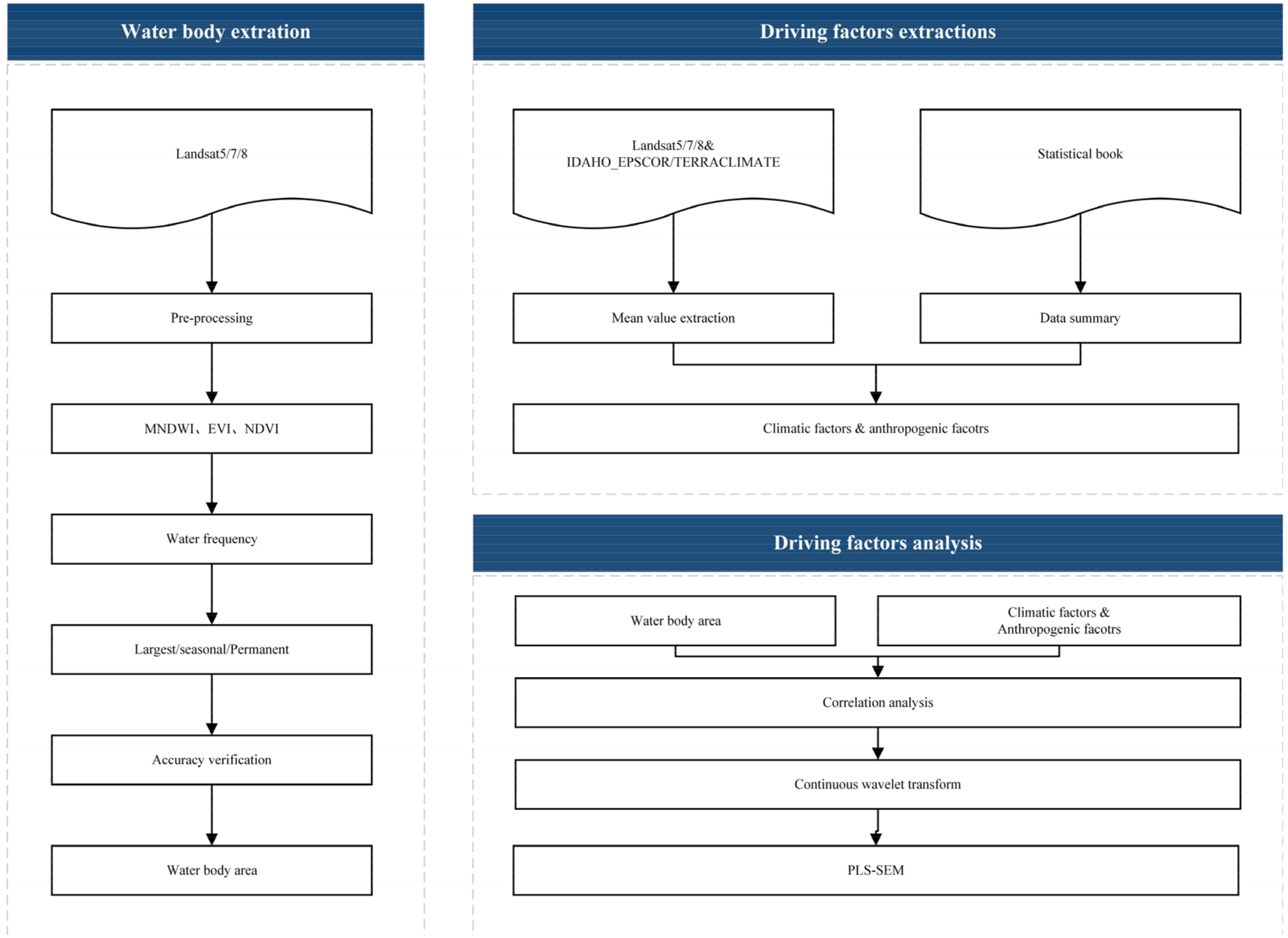
2.8. Conceptual Framework and Procedures of the Study

Figure 2 shows the conceptual framework of this study.

The first step is water body extraction. Initially, Landsat images are preprocessed using the Google Earth Engine (GEE) platform. Then, based on water extraction rules and water frequency, three different types of water bodies are extracted. Subsequently, data processing is conducted on the ArcMap platform to obtain lake area data.

The second step is obtaining driving factors. This involves processing Earth Engine’s public data/IDAHO_EPSCOR/TERRACLIMATE, Landsat images, and statistical yearbook data to organize and obtain the data related to driving factors.

The final step involves the analysis of driving factors. By combining coherence analysis and continuous wavelet transform analysis results, a structural equation model is constructed to quantitatively explain the impact of driving factors on changes in lake area.

3. Results

3.1. Evaluation of Water Body Extraction Accuracy

As shown in

Table 2. Evaluation table of accuracy of water body information extraction results. Overall Accuracy (OA), and Kappa coefficient (KC) to evaluate the accuracy of water bodies in the Jianghan Plain.

	Samples	Google Earth		Total	User’s Accuracy
		Water	Non-Water
Landsat	Water body	943	57	1000	94.30%
	Non-water body	60	940	1000	94.00%
Total		1003	997	2000	Overall accuracy = 94.15%
Producer’s accuracy		94.02%	94.28%		Kappa coefficient = 0.861

, by computing the confusion matrix, the overall accuracy of the water body identification algorithm in the Jianghan Plain has reached 94.15%. Moreover, with a Kappa coefficient of 0.86, exceeding 0.8, it indicates that the algorithm’s accuracy in identifying water bodies in the Jianghan Plain is high when utilizing remote sensing vegetation indices and water indices, allowing for batch extraction of Jianghan Plain water bodies across different time series.

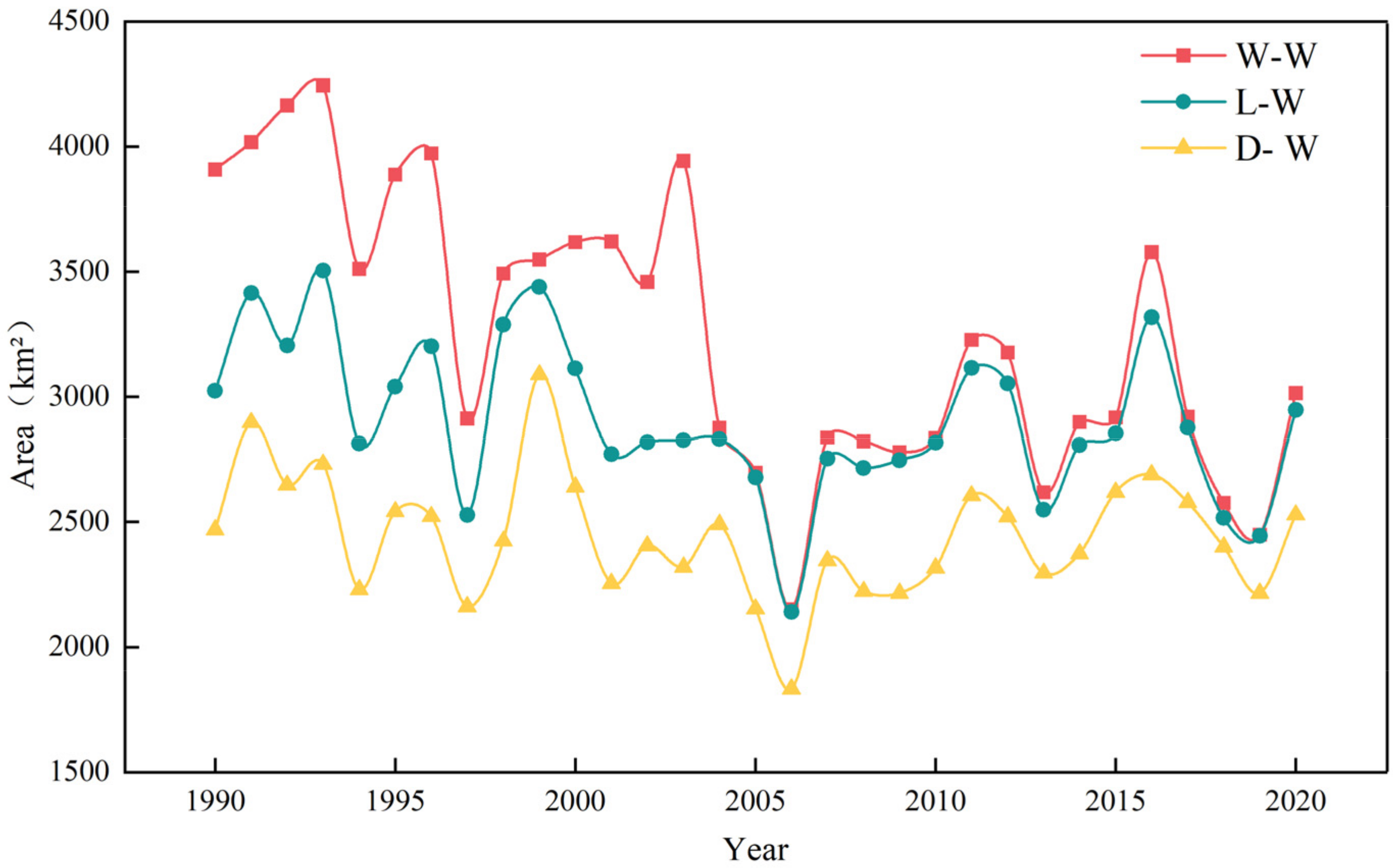
3.2. Characteristics of Changes in Area of the Lakes of Jianghan Plain

By using the aforementioned water body extraction algorithm and combining visual interpretation, lakes with an area greater than 1 km² in the Jianghan Plain area were extracted annually from 1990 to 2020. These lakes were classified into the following categories based on different water body frequencies: the wet seasonal lakes, the level seasonal lakes, and the dry seasonal lakes. According to the extraction results, the lakes in the Jianghan Plain exhibit the following characteristics in terms of area changes (Figure 3 and Figure 4).

As shown in Figure 4, for the lake area of the wet seasonal lakes (W-W) and the level seasonal lakes (L-W), the trend of lake area change shows an initial increase followed by a decrease. However, for the lake area of the dry seasonal lakes (D-W), the trend of lake area change shows an initial increase, followed by a decrease, then an increase again, and finally another decrease.

The largest lake area of the wet seasonal lakes (W-W) was 4244.765 km² in 1993, and the smallest was 2151.441 km² in 2006. The total decrease in area from 1990 to 2020 was 893.1 km², with a decrease rate of 28 km²/year. The largest lake area of the level seasonal lakes (L-W) was 3504.553 km² in 1993, and the smallest was 2140.046 km² in 2006. The total decrease in area from 1990 to 2020 was 77.9 km², with a decrease rate of 2.5 km²/year. The largest lake area of the dry seasonal lakes (D-W) was 3088.72 km² in 1999, and the smallest was 1833.67 km² in 2006. The total increase in area from 1990 to 2020 was 59.27 km², with an increase rate of 1.9 km²/year.

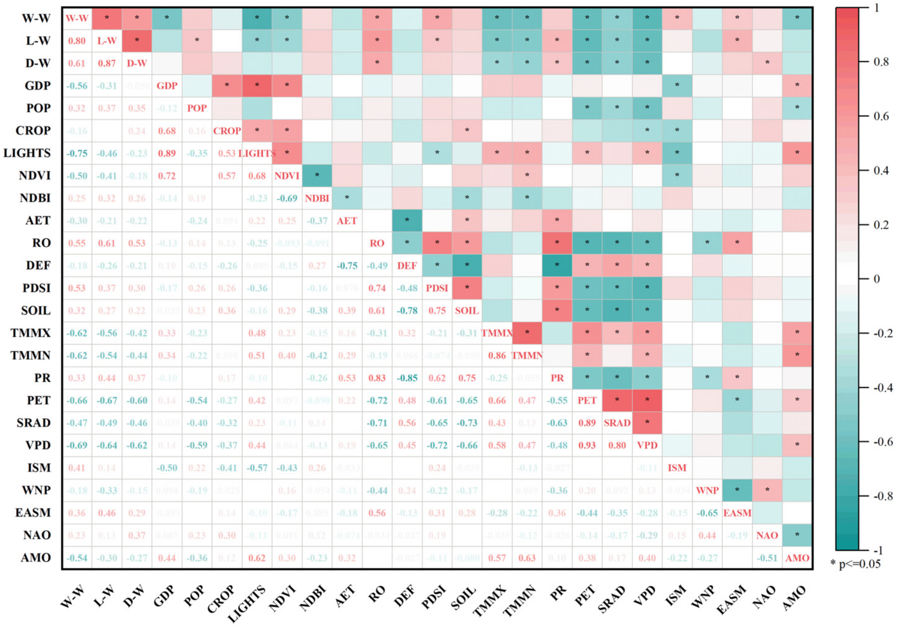
3.3. The Pearson Correlation between Changes in Lake Area and Driving Factors

As shown in Figure 5, the areas of the three types of lakes are significantly negatively correlated with factors such as TMMX, TMMN, PET, SRAD, and VPD, while they are significantly positively correlated with the RO factor.

3.3.1. The Pearson Correlation between the Area of the Wet Seasonal Lake and the Driving Factors

In terms of human factors, the area of the wet seasonal lake exhibits significant negative correlations with GDP, LIGHTS, NDVI, and CROP, while showing positive correlations with POP and NDBI. In terms of natural factors, the area of the largest lake shows significant negative correlations with TMMX, TMMN, PET, SRAD, VPD, and AMO, while exhibiting significant positive correlations with RO, PDSI, ISM, EASM, and NAO. Additionally, it shows negative correlations with AET, DEF, and WNP, and positive correlations with SOIL, PR, and NAO.

3.3.2. The Pearson Correlation between the Area of Level Seasonal Lakes and Driving Factors

In terms of human factors, the area of seasonal lakes exhibits a significant negative correlation with LIGHTS and NDVI, a significant positive correlation with population (POP), and a negative correlation with GDP, with a weaker correlation with CROP. In terms of natural factors, the area of level seasonal lakes shows a significant negative correlation with TMMX, TMMN, PET, SRAD, and VPD. It exhibits a significant positive correlation with RO, PDSI, PR, and EASM. Additionally, it demonstrates a negative correlation with AET, DEF, WNP, and AMO, and a positive correlation with SOIL, ISM, and NAO.

3.3.3. The Pearson Correlation between the Area of Dry Seasonal Lakes and Driving Factors

In terms of human factors, the area of dry seasonal lakes shows a positive correlation with POP, CROP, and NDBI, while exhibiting negative correlations with LIGHTS and NDVI, with GDP showing a weaker correlation. In terms of natural factors, the area of permanent lakes shows a significant negative correlation with TMMX, TMMN, PET, SRAD, and VPD, while showing significant positive correlations with PR, and NAO. It exhibits negative correlations with AET, DEF, WNP, and AMO, and positive correlations with PDSI and soil EASM. The correlation with ISM is not high.

Therefore, the following conclusions can be drawn. (1) In terms of different types of influencing factors, human elements primarily affect the changes in the wet and level seasonal lake areas, while the area changes of dry seasonal lakes are mainly governed by natural factors. (2) In terms of spatial scale of influencing factors, at smaller scales, environmental factors exert similar effects on the area changes of the three types of lakes, with natural elements like RO and SRAD showing strong correlations. However, at larger spatial scales, different environmental factors exhibit varying correlations with the three types of lakes. The area changes of the wet seasonal lakes are strongly correlated with a wider range of remote sensing indices, while the level seasonal lakes and the dry seasonal lakes are strongly correlated with EASM and NAO, respectively.

3.4. Drivers of Water Body Area Based on PLS-SEM

Further integrating the results of the Continuous Wavelet Transform (CWT) (Figure 6), during the period from 1995 to 2000, there was a strong fluctuation cycle of approximately 2 years in lake area changes, as indicated by the yellow region within the solid black line. It is closely associated with human factors such as POP, NDVI, and NDBI, as well as climate factors like AET, RO, and PDSI. They exhibit similar cyclic variations to the changes in lake area. Combining correlation analysis, GDP, LIGHTS, and NDVI were selected as latent variables for human factors, while RO, PDSI, SOIL, TMMX, TMMN, PR, PET, SRAD, VPD, and EASM were chosen as latent variables for environmental factors to construct the structural equation model, eliminating redundancy in the driving factors.

Through correlation analysis and mutation tests, to better explain changes in lake area, the driving factors influencing lake area changes were divided into four latent variables: human factors, climatic factors, remote sensing factors, and hydrologic factors. Based on this, a structural equation model was constructed.

Through structural equation modeling (Figure 7), the path coefficients of each latent variable on water area change are determined. The PLS-SEM model can display the contribution of each latent variable to water area change. As shown in

Table 3. The path coefficients of observed variables.

Name	Block	W-W	L-W	D-W
GDP	Human	0.323	0.276	0.154
LIGHTS	Human	0.529	0.547	0.742
NDVI	Human	0.221	0.254	0.159
EASM	Remote	1.000	1.000	1.000
PDSI	Climate	−0.232	0.210	0.210
TMMX	Climate	0.178	−0.172	−0.156
TMMN	Climate	0.134	−0.124	−0.113
PR	Climate	−0.202	0.229	0.230
PET	Climate	0.263	−0.273	−0.278
VPD	Climate	0.258	−0.257	−0.270
SOIL	Hydrologic	0.296	0.282	0.284
RO	Hydrologic	0.453	0.465	0.454
SRAD	Hydrologic	−0.375	−0.376	−0.385

, the path coefficients of each observed variable to the latent variable can be observed.

3.4.1. The Wet Seasonal Lake Structural Equation Model

The overall fit is 0.74, exceeding 0.7, indicating a good fit. During this period, the influences of human, hydrologic, and climate factors on lake area change are negatively correlated, while the remote factor is positively correlated. Additionally, the influence of the remote factor is smaller than the other three factors. Climate is the most influential latent variable. Within the climate latent variable, precipitation (PR) and the Palmer Drought Severity Index (PDSI) have a positive correlation with climate change, while vapor pressure deficit (VPD), potential evapotranspiration (PET), maximum temperature (TMMX), and minimum temperature (TMMN) have a negative correlation. In the models of the remaining latent variables, all observed variables have a positive correlation with their respective latent variables, except for shortwave radiation (SRAD) in the hydrologic latent variable, which has a negative correlation.

3.4.2. The Level Seasonal Lake Structural Equation Model

The overall fit of the model is 0.70, which is equal to or greater than 0.7, indicating a good fit. During this period, the effects of hydrologic and climate factors on lake area change are negatively correlated, while those of human and remote factors are positively correlated. Climate is the most influential latent variable. Within the climate latent variable, vapor pressure deficit (VPD), potential evapotranspiration (PET), maximum temperature (TMMX), and minimum temperature (TMMN) show positive correlations, while precipitation (PR) and the Palmer Drought Severity Index (PDSI) exhibit negative correlations with climate change. The correlation of observed variables in the remaining latent variable models is similar to that in the model of the wet seasonal lake.

3.4.3. The Dry Seasonal Lake Structural Equation Model

The overall fit is 0.65, greater than 0.6 but less than 0.7, indicating a relatively good fit. During this period, the effects of human, hydrologic, and climate factors show negative correlations with the change in lake area, while the remote factor exhibits a positive correlation. Climate remains the most influential latent variable; however, the remote factor’s influence, as indicated by the absolute values of path coefficients, has increased and is second only to climate. Additionally, the correlations between observed variables in each latent variable model are similar to those in the model for the wet seasonal lake.

From this, the following conclusions can be drawn. (1) The overall fit of the models for the three different periods are 0.74, 0.70, and 0.65, respectively. Generally, the models exhibit a good fit, with the structural equation model showing the greatest explanatory power for the changes in area during the period of the largest lake. (2) In terms of the factors influencing the models, the path coefficients of the remote factor for the lake area change are positive, while those of the climate and hydrologic factors for the lake area change in the three different periods are negative. The human factor exhibits different correlations with the lakes in different periods: negative correlation during the wet seasonal lake and the dry seasonal lake periods, and positive correlation during the level seasonal lake period, with path coefficients of −0.452, 0.112, and −0.192, respectively. The path coefficients of the climate factor are −0.706, −0.944, and −0.723, respectively. Considering the absolute values and signs of the comprehensive path coefficients, it indicates that environmental factors are the main contributors to the continuous changes in lake area, and the impact of human factors on lake area change is smaller than that of environmental and hydrologic factors. However human factors mainly influence the mutation of the lakes’ area.

4. Discussion

4.1. Water Extraction

This study combines the use of the MNDWI, NDVI, and EVI to extract water bodies at different thresholds. In this study, the results from the confusion matrix showed an overall accuracy of 94.15%, with a kappa coefficient of 0.86. Therefore, it can be considered that the extraction results are quite satisfactory [62]. In practice, the field of remote sensing water body extraction often employs various machine learning classification techniques, However, classification methods typically require a large number of interested sample points [71,72,73]. The Jianghan Lake Basin has complex terrain and diverse land types, which greatly affect the quality of classification results and classification rules, leading to low efficiency in water body extraction. Therefore, in the research process, based on the Google Earth Engine (GEE) platform, the water index method remains a fast and accurate method for extracting water bodies over a long period of time [26]. Visual discrimination based on the results of water body extraction improves the efficiency and accuracy of lake identification [42].

By observing the results of water body extraction, it was noticed that the minimum values of the three types of lakes in terms of area and quantity all occurred in 2006. The main reason for this was the completion and operation of the large-scale hydraulic project, the Three Gorges Dam, in 2006, which affected the area of water resources in the downstream Jianghan Plain and led to a decrease in water area [74]. Later, with the introduction of the new concept of ecological civilization development, the country implemented measures such as returning farmland to forests to improve the ecological environment of water bodies. These measures had a positive effect on the expansion of water body areas in the Jianghan Plain, leading to further enlargement of water body areas [53].

4.2. Driving Factors of Water Area Change

In terms of the types of influencing factors, human factors mainly affect the area of the wet seasonal lakes and the level seasonal lakes, while their impact on the dry seasonal lakes is relatively minor. The reason for this is that these two types of water bodies have larger water areas at the spatial scale, making them more susceptible to various human activities. During the wet seasonal lakes and the level seasonal lakes periods, lakes exhibit augmented water volume and elevated water levels, leading to an expansion of lake surface area. Human activities can exacerbate this phenomenon, notably through interventions such as river diversion and dam construction aimed at water level regulation, thereby exerting influence on lake extent [75]. In contrast, the dry seasonal lakes period corresponds to a relatively reduced lake surface area and lower water levels. Consequently, human activities exert a comparatively diminished impact on lake area during this period. Even activities such as land reclamation may yield limited effects due to constrained water availability [76].

Furthermore, in terms of the spatial scale of influencing factors, the reason why the wet seasonal lakes show a significant correlation with more remote sensing indices compared to the level seasonal and the dry seasonal lakes is because the area of the wet seasonal lakes is broader. Remote sensing indices include various monsoon elements, and the larger water area of the largest lakes allows for more exposure to monsoon climates [77]. Therefore, at a larger scale, the largest lakes exhibit significant correlations with more remote sensing indices.

4.3. Applicability of Structural Equation Models

In terms of the overall fit of the models, the high goodness-of-fit of the structural equation models for the three types of lakes can be attributed to several factors. Firstly, significant correlated factors were selected based on correlation analysis. Secondly, in addition to selecting highly correlated factors, continuous wavelet transform was also incorporated to identify factors with similar trends [65,66,67]. By combining correlation analysis with continuous wavelet transform analysis, relevant factors can be effectively identified, thus enabling the construction of a structural equation model [43].

In terms of the factors influencing the models, the dominance of climate factors in driving continuous changes of area across the three types of water bodies is attributed to the inclusion of key factors such as evaporation, temperature, and precipitation within the climate variables. These factors are critical factors affecting the changes in lake area in the study area [27]. Generally, evaporation has a negative impact on lake area; the greater the evaporation from the lake surface, the more severe the loss of water from the lake, resulting in a reduction in lake area. Higher temperatures lead to enhanced lake surface evaporation, consequently causing a decrease in lake area [27]. Increased precipitation directly adds water to the lake or collects water from surrounding areas, resulting in an increase in lake area [52].

Another issue worth discussing is why the Three Gorges Dam is considered the main factor driving mutation in water area but does not appear to be reflected in the structural equation model. Upon observing the trend of water body area changes, it is evident that all three types of lakes experienced a sudden decrease in area around 2006. One reason for this discrepancy is the difficulty in directly selecting a representative indicator to signify the completion of the Three Gorges Dam project. Over a thirty-year time frame, its construction represents a singular event, making it challenging to incorporate into the analysis of the structural equation model [43]. Another reason may be that the primary function of the Three Gorges Dam is to regulate water bodies for various purposes. Although some water bodies are impounded by the dam, the remaining water bodies still primarily participate in hydrological cycles through processes such as temperature, precipitation, and evaporation. Therefore, despite the completion and operation of the Three Gorges Dam being a significant cause of the sharp decrease in water body area, the environmental factors remain the predominant drivers of continuous changes in the overall lake area in the Jianghan Plain [74,78,79].

4.4. Limitations of the Study and Prospects

In terms of the temporal scale of the research content, due to limitations in climate and climate data availability, this study only explored the changes in lake area in the Jianghan Plain from 1990 to 2020 and investigated its driving factors, failing to achieve research on a longer time scale.

In terms of the selection of elements in the research content, although significant remote sensing indices were selected to investigate their influence on lake changes at a larger spatial scale, a series of extreme weather and climate events affecting lake area changes were difficult to quantitatively analyze [55,56,57,58,59]. Additionally, limitations in the precision of the dataset itself may also impose constraints on the research conclusions [55,56,57,58,59].

In the future, with the further development of image recognition technology, the production of higher-precision remote sensing image products may advance the understanding of dynamic changes in the Jianghan Plain lakes [26].

5. Conclusions

This study utilized the GEE platform and structural equation modeling to explore the dynamic trends of lake area changes in different types of lakes in the Jianghan Plain from 1990 to 2020, as well as the primary drivers of lake area variation. In terms of the trend of changes in lake area for different types of lakes, the water bodies of different types exhibited varying trends in overall area changes. The area of the wet seasonal lake and the level seasonal lake showed a decreasing trend, decreasing by 893.1 km² and 77.9 km², respectively. Conversely, the area of the dry lake increased by 59.27 km². The areas of all three types reached their minimum values in 2006. In terms of dynamic change influencing factors, human factors primarily affect the variation in water body area of the wet seasonal lakes in the Jianghan Plain, while the level seasonal and the dry lake bodies are mainly regulated by climate factors. And it was found that climate factors are the dominant drivers of lake area continuous changes in the Jianghan Plain over the three different periods, and human factors mainly influence the mutation of lakes area. The results of this study enhance our understanding of the impact of surface water changes in the Jianghan Plain and provide important references for the monitoring and restoration of water resources over long time series.

References

1. Donchyts, G.; Baart, F.; Winsemius, H.; Gorelick, N.; Kwadijk, J.; Van De Giesen, N. Earth’s Surface Water Change over the Past 30 Years. Nat. Clim. Chang. 2016, 6, 810–813. [Google Scholar] [CrossRef]
2. Jiang, Z.; Jiang, W.; Ling, Z.; Wang, X.; Peng, K.; Wang, C. Surface Water Extraction and Dynamic Analysis of Baiyangdian Lake Based on the Google Earth Engine Platform Using Sentinel-1 for Reporting SDG 6.6.1 Indicators. Water 2021, 13, 138. [Google Scholar] [CrossRef]
3. Bo, Y.; Zhou, F.; Zhao, J.; Liu, J.; Liu, J.; Ciais, P.; Chang, J.; Chen, L. Additional Surface-Water Deficit to Meet Global Universal Water Accessibility by 2030. J. Clean. Prod. 2021, 320, 128829. [Google Scholar] [CrossRef]
4. Koning, C.O. Vegetation Patterns Resulting from Spatial and Temporal Variability in Hydrology, Soils, and Trampling in an Isolated Basin Marsh, New Hampshire, USA. Wetlands 2005, 25, 239–251. [Google Scholar] [CrossRef]
5. Robledano, F.; Esteve, M.A.; Farinós, P.; Carreño, M.F.; Martínez-Fernández, J. Terrestrial Birds as Indicators of Agricultural-Induced Changes and Associated Loss in Conservation Value of Mediterranean Wetlands. Ecol. Indic. 2010, 10, 274–286. [Google Scholar] [CrossRef]
6. Pekel, J.-F.; Cottam, A.; Gorelick, N.; Belward, A.S. High-Resolution Mapping of Global Surface Water and Its Long-Term Changes. Nature 2016, 540, 418–422. [Google Scholar] [CrossRef] [PubMed]
7. Li, X.; Zhang, F.; Shi, J.; Chan, N.W.; Cai, Y.; Cheng, C.; An, C.; Wang, W.; Liu, C. Analysis of Surface Water Area Dynamics and Driving Forces in the Bosten Lake Basin Based on GEE and SEM for the Period 2000 to 2021. Env. Sci. Pollut. Res. 2024, 31, 9333–9346. [Google Scholar] [CrossRef] [PubMed]
8. Khandelwal, A.; Karpatne, A.; Marlier, M.E.; Kim, J.; Lettenmaier, D.P.; Kumar, V. An Approach for Global Monitoring of Surface Water Extent Variations in Reservoirs Using MODIS Data. Remote Sens. Environ. 2017, 202, 113–128. [Google Scholar] [CrossRef]
9. Li, L.; Vrieling, A.; Skidmore, A.; Wang, T.; Turak, E. Monitoring the Dynamics of Surface Water Fraction from MODIS Time Series in a Mediterranean Environment. Int. J. Appl. Earth Obs. Geoinf. 2018, 66, 135–145. [Google Scholar] [CrossRef]
10. Lu, S.; Jia, L.; Zhang, L.; Wei, Y.; Baig, M.H.A.; Zhai, Z.; Meng, J.; Li, X.; Zhang, G. Lake Water Surface Mapping in the Tibetan Plateau Using the MODIS MOD09Q1 Product. Remote Sens. Lett. 2017, 8, 224–233. [Google Scholar] [CrossRef]
11. Ranghetti, L.; Busetto, L.; Crema, A.; Fasola, M.; Cardarelli, E.; Boschetti, M. Testing Estimation of Water Surface in Italian Rice District from MODIS Satellite Data. Int. J. Appl. Earth Obs. Geoinf. 2016, 52, 284–295. [Google Scholar] [CrossRef]
12. Zhang, Y.; Shi, K.; Zhou, Y.; Liu, X.; Qin, B. Monitoring the River Plume Induced by Heavy Rainfall Events in Large, Shallow, Lake Taihu Using MODIS 250m Imagery. Remote Sens. Environ. 2016, 173, 109–121. [Google Scholar] [CrossRef]
13. Jia, K.; Jiang, W.; Li, J.; Tang, Z. Spectral Matching Based on Discrete Particle Swarm Optimization: A New Method for Terrestrial Water Body Extraction Using Multi-Temporal Landsat 8 Images. Remote Sens. Environ. 2018, 209, 1–18. [Google Scholar] [CrossRef]
14. Tulbure, M.G.; Broich, M. Spatiotemporal Patterns and Effects of Climate and Land Use on Surface Water Extent Dynamics in a Dryland Region with Three Decades of Landsat Satellite Data. Sci. Total Environ. 2019, 658, 1574–1585. [Google Scholar] [CrossRef] [PubMed]
15. Li, L.; Chen, Y.; Xu, T.; Liu, R.; Shi, K.; Huang, C. Super-Resolution Mapping of Wetland Inundation from Remote Sensing Imagery Based on Integration of Back-Propagation Neural Network and Genetic Algorithm. Remote Sens. Environ. 2015, 164, 142–154. [Google Scholar] [CrossRef]
16. Wang, X.; Xie, S.; Zhang, X.; Chen, C.; Guo, H.; Du, J.; Duan, Z. A Robust Multi-Band Water Index (MBWI) for Automated Extraction of Surface Water from Landsat 8 OLI Imagery. Int. J. Appl. Earth Obs. Geoinf. 2018, 68, 73–91. [Google Scholar] [CrossRef]
17. Hardy, A.; Ettritch, G.; Cross, D.; Bunting, P.; Liywalii, F.; Sakala, J.; Silumesii, A.; Singini, D.; Smith, M.; Willis, T.; et al. Automatic Detection of Open and Vegetated Water Bodies Using Sentinel 1 to Map African Malaria Vector Mosquito Breeding Habitats. Remote Sens. 2019, 11, 593. [Google Scholar] [CrossRef]
18. Schwatke, C.; Scherer, D.; Dettmering, D. Automated Extraction of Consistent Time-Variable Water Surfaces of Lakes and Reservoirs Based on Landsat and Sentinel-2. Remote Sens. 2019, 11, 1010. [Google Scholar] [CrossRef]
19. Steinhausen, M.J.; Wagner, P.D.; Narasimhan, B.; Waske, B. Combining Sentinel-1 and Sentinel-2 Data for Improved Land Use and Land Cover Mapping of Monsoon Regions. Int. J. Appl. Earth Obs. Geoinf. 2018, 73, 595–604. [Google Scholar] [CrossRef]
20. Wang, C.; Jia, M.; Chen, N.; Wang, W. Long-Term Surface Water Dynamics Analysis Based on Landsat Imagery and the Google Earth Engine Platform: A Case Study in the Middle Yangtze River Basin. Remote Sens. 2018, 10, 1635. [Google Scholar] [CrossRef]
21. Gorelick, N.; Hancher, M.; Dixon, M.; Ilyushchenko, S.; Thau, D.; Moore, R. Google Earth Engine: Planetary-Scale Geospatial Analysis for Everyone. Remote Sens. Environ. 2017, 202, 18–27. [Google Scholar] [CrossRef]
22. Oliphant, A.J.; Thenkabail, P.S.; Teluguntla, P.; Xiong, J.; Gumma, M.K.; Congalton, R.G.; Yadav, K. Mapping Cropland Extent of Southeast and Northeast Asia Using Multi-Year Time-Series Landsat 30-m Data Using a Random Forest Classifier on the Google Earth Engine Cloud. Int. J. Appl. Earth Obs. Geoinf. 2019, 81, 110–124. [Google Scholar] [CrossRef]
23. Kumar, L.; Mutanga, O. Google Earth Engine Applications Since Inception: Usage, Trends, and Potential. Remote Sens. 2018, 10, 1509. [Google Scholar] [CrossRef]
24. Hird, J.; DeLancey, E.; McDermid, G.; Kariyeva, J. Google Earth Engine, Open-Access Satellite Data, and Machine Learning in Support of Large-Area Probabilistic Wetland Mapping. Remote Sens. 2017, 9, 1315. [Google Scholar] [CrossRef]
25. Ismail, M.A.; Waqas, M.; Ali, A.; Muzzamil, M.M.; Abid, U.; Zia, T. Enhanced Index for Water Body Delineation and Area Calculation Using Google Earth Engine: A Case Study of the Manchar Lake. J. Water Clim. Chang. 2022, 13, 557–573. [Google Scholar] [CrossRef]
26. Zou, Z.; Xiao, X.; Dong, J.; Qin, Y.; Doughty, R.B.; Menarguez, M.A.; Zhang, G.; Wang, J. Divergent Trends of Open-Surface Water Body Area in the Contiguous United States from 1984 to 2016. Proc. Natl. Acad. Sci. USA 2018, 115, 3810–3815. [Google Scholar] [CrossRef] [PubMed]
27. Chai, X.R.; Li, M.; Wang, G.W. Characterizing Surface Water Changes across the Tibetan Plateau Based on Landsat Time Series and LandTrendr Algorithm. Eur. J. Remote Sens. 2022, 55, 251–262. [Google Scholar] [CrossRef]
28. Deng, Y.; Jiang, W.; Tang, Z.; Ling, Z.; Wu, Z. Long-Term Changes of Open-Surface Water Bodies in the Yangtze River Basin Based on the Google Earth Engine Cloud Platform. Remote Sens. 2019, 11, 2213. [Google Scholar] [CrossRef]
29. Tulbure, M.G.; Broich, M.; Stehman, S.V.; Kommareddy, A. Surface Water Extent Dynamics from Three Decades of Seasonally Continuous Landsat Time Series at Subcontinental Scale in a Semi-Arid Region. Remote Sens. Environ. 2016, 178, 142–157. [Google Scholar] [CrossRef]
30. Yang, X.; Zhao, S.; Qin, X.; Zhao, N.; Liang, L. Mapping of Urban Surface Water Bodies from Sentinel-2 MSI Imagery at 10 m Resolution via NDWI-Based Image Sharpening. Remote Sens. 2017, 9, 596. [Google Scholar] [CrossRef]
31. Wang, X.; Liu, Y.; Ling, F.; Liu, Y.; Fang, F. Spatio-Temporal Change Detection of Ningbo Coastline Using Landsat Time-Series Images during 1976–2015. ISPRS Int. J. Geo-Inf. 2017, 6, 68. [Google Scholar] [CrossRef]
32. Cavallo, C.; Papa, M.N.; Gargiulo, M.; Palau-Salvador, G.; Vezza, P.; Ruello, G. Continuous Monitoring of the Flooding Dynamics in the Albufera Wetland (Spain) by Landsat-8 and Sentinel-2 Datasets. Remote Sens. 2021, 13, 3525. [Google Scholar] [CrossRef]
33. McFeeters, S.K. The Use of the Normalized Difference Water Index (NDWI) in the Delineation of Open Water Features. Int. J. Remote Sens. 1996, 17, 1425–1432. [Google Scholar] [CrossRef]
34. Xu, H. Modification of Normalised Difference Water Index (NDWI) to Enhance Open Water Features in Remotely Sensed Imagery. Int. J. Remote Sens. 2006, 27, 3025–3033. [Google Scholar] [CrossRef]
35. Feyisa, G.L.; Meilby, H.; Fensholt, R.; Proud, S.R. Automated Water Extraction Index: A New Technique for Surface Water Mapping Using Landsat Imagery. Remote Sens. Environ. 2014, 140, 23–35. [Google Scholar] [CrossRef]
36. Wu, X.; Kumar, V.; Quinlan, J.R.; Ghosh, J.; Yang, Q.; Motoda, H.; McLachlan, G.J.; Ng, A.; Liu, B.; Yu, P.S.; et al. Top 10 Algorithms in Data Mining. Knowl. Inf. Syst. 2008, 14, 1–37. [Google Scholar] [CrossRef]
37. Cortes, C.; Vapnik, V. Support-vector networks. Mach. Learn. 1995, 20, 273–297. [Google Scholar] [CrossRef]
38. Chen, T.; Guestrin, C. Assoc Comp Machinery XGBoost: A Scalable Tree Boosting System. In Proceedings of the 22nd ACM Sigkdd International Conference on Knowledge Discovery and Data Mining, San Francisco, CA, USA, 13–17 August 2016; pp. 785–794. [Google Scholar]
39. Belgiu, M.; Dragut, L. Random Forest in Remote Sensing: A Review of Applications and Future Directions. ISPRS J. Photogramm. Remote Sens. 2016, 114, 24–31. [Google Scholar] [CrossRef]
40. Tucker, C.J. Red and Photographic Infrared Linear Combinations for Monitoring Vegetation. Remote Sens. Environ. 1979, 8, 127–150. [Google Scholar] [CrossRef]
41. Huete, A.; Didan, K.; Miura, T.; Rodriguez, E.P.; Gao, X.; Ferreira, L.G. Overview of the Radiometric and Biophysical Performance of the MODIS Vegetation Indices. Remote Sens. Environ. 2002, 83, 195–213. [Google Scholar] [CrossRef]
42. Zhou, Y.; Dong, J.; Xiao, X.; Liu, R.; Zou, Z.; Zhao, G.; Ge, Q. Continuous Monitoring of Lake Dynamics on the Mongolian Plateau Using All Available Landsat Imagery and Google Earth Engine. Sci. Total Environ. 2019, 689, 366–380. [Google Scholar] [CrossRef] [PubMed]
43. Shipley, B. A New Inferential Test for Path Models Based on Directed Acyclic Graphs. Struct. Equ. Model. A Multidiscip. J. 2000, 7, 206–218. [Google Scholar] [CrossRef]
44. Tenenhaus, M.; Amato, S.; Vinzi, V.E. A Global Goodness-of-Fit Index for PLS Structural Equation Modelling. Proc. XLII SIS Sci. Meet. 2004, 1, 739–742. [Google Scholar]
45. Wang, W.; Zhang, F.; Zhao, Q.; Liu, C.; Jim, C.Y.; Johnson, V.C.; Tan, M.L. Determining the Main Contributing Factors to Nutrient Concentration in Rivers in Arid Northwest China Using Partial Least Squares Structural Equation Modeling. J. Environ. Manag. 2023, 343, 118249. [Google Scholar] [CrossRef] [PubMed]
46. Hair, J.F.; Ringle, C.M.; Sarstedt, M. PLS-SEM: Indeed a Silver Bullet. J. Mark. Theory Pract. 2011, 19, 139–152. [Google Scholar] [CrossRef]
47. Liu, J.; Zeng, M.; Wang, D.; Zhang, Y.; Shang, B.; Ma, X. Applying Social Cognitive Theory in Predicting Physical Activity Among Chinese Adolescents: A Cross-Sectional Study With Multigroup Structural Equation Model. Front. Psychol. 2022, 12, 695241. [Google Scholar] [CrossRef] [PubMed]
48. Wang, C.; Ma, L.; Zhang, Y.; Chen, N.; Wang, W. Spatiotemporal Dynamics of Wetlands and Their Driving Factors Based on PLS-SEM: A Case Study in Wuhan. Sci. Total Environ. 2022, 806, 151310. [Google Scholar] [CrossRef] [PubMed]
49. Ahmed, T.; Chandran, V.G.R.; Klobas, J.E.; Liñán, F.; Kokkalis, P. Entrepreneurship Education Programmes: How Learning, Inspiration and Resources Affect Intentions for New Venture Creation in a Developing Economy. Int. J. Manag. Educ. 2020, 18, 100327. [Google Scholar] [CrossRef]
50. Cheng, C.; Zhang, F.; Tan, M.L.; Kung, H.-T.; Shi, J.; Zhao, Q.; Wang, W.; Duan, P.; An, C.; Cai, Y.; et al. Characteristics of Dissolved Organic Matter and Its Relationship with Water Quality along the Downstream of the Kaidu River in China. Water 2022, 14, 3544. [Google Scholar] [CrossRef]
51. Chang, T.; Li, J.; Guo, X.; Li, Y. The Spatial-Temporal Characteristics and Driving Forces Analysis of Water Area Landscape Pattern Changes on the Jianghan Plain. Adv. Water Sci. 2023, 34, 21–32. [Google Scholar]
52. Wei, W.; Tang, L.; Ma, R. Evolution and Controlling Factors of Wetlands in Jianghan Plain. Saf. Environ. Eng. 2021, 28, 25–33. [Google Scholar]
53. Feng, W.; Feng, C.; Chen, J. Effect of Human Activities and Association Rules Mining on Spatiotemporal Evolution in Jianghan Lake Group. J. Appl. Sci. 2018, 36, 958–968. [Google Scholar]
54. Song, L.; Song, C.; Luo, S.; Chen, T.; Liu, K.; Zhang, Y.; Ke, L. Integrating ICESat-2 Altimetry and Machine Learning to Estimate the Seasonal Water Level and Storage Variations of National-Scale Lakes in China. Remote Sens. Environ. 2023, 294, 113657. [Google Scholar] [CrossRef]
55. Vicente-Serrano, S.; Beguería, S.; López-Moreno, J. A Multiscalar Drought Index Sensitive to Global Warming: The Standardized Precipitation Evapotranspiration Index. J. Clim. 2010, 23, 1696–1718. [Google Scholar] [CrossRef]
56. Wang, B.; Wu, R.; Lau, K. Interannual Variability of the Asian Summer Monsoon: Contrasts between the Indian and the Western North Pacific-East Asian Monsoons. J. Clim. 2001, 14, 4073–4090. [Google Scholar] [CrossRef]
57. Li, J.; Zeng, Q. A Unified Monsoon Index. Geophys. Res. Lett. 2002, 29, 115. [Google Scholar] [CrossRef]
58. Hurrell, J. Decadal trends in the north-atlantic oscillation—Regional temperatures and precipitation. Science 1995, 269, 676–679. [Google Scholar] [CrossRef] [PubMed]
59. Enfield, D.; Mestas-Nuñez, A.; Trimble, P. The Atlantic Multidecadal Oscillation and Its Relation to Rainfall and River Flows in the Continental US. Geophys. Res. Lett. 2001, 28, 2077–2080. [Google Scholar] [CrossRef]
60. Zhang, L.; Ren, Z.; Chen, B.; Gong, P.; Xu, B.; Fu, H. A Prolonged Artificial Nighttime-Light Dataset of China (1984–2020). Sci. Data 2024, 11, 414. [Google Scholar] [CrossRef] [PubMed]
61. Zha, Y.; Gao, J.; Ni, S. Use of Normalized Difference Built-up Index in Automatically Mapping Urban Areas from TM Imagery. Int. J. Remote Sens. 2003, 24, 583–594. [Google Scholar] [CrossRef]
62. Chen, T.; Song, C.; Fan, C.; Cheng, J.; Duan, X.; Wang, L.; Liu, K.; Deng, S.; Che, Y. A Comprehensive Data Set of Physical and Human-Dimensional Attributes for China’s Lake Basins. Sci. Data 2022, 9, 519. [Google Scholar] [CrossRef] [PubMed]
63. Wang, J. Determining the Most Accurate Program for the Mann-Kendall Method in Detecting Climate Mutation. Theor. Appl. Clim. 2020, 142, 847–854. [Google Scholar] [CrossRef]
64. Guo, M.; Li, J.; He, H.; Xu, J.; Jin, Y. Detecting Global Vegetation Changes Using Mann-Kendal (MK) Trend Test for 1982–2015 Time Period. Chin. Geogr. Sci. 2018, 28, 907–919. [Google Scholar] [CrossRef]
65. Martínez, B.; Gilabert, M.A. Vegetation Dynamics from NDVI Time Series Analysis Using the Wavelet Transform. Remote Sens. Environ. 2009, 113, 1823–1842. [Google Scholar] [CrossRef]
66. Quiroz, R. Improving Daily Rainfall Estimation from NDVI Using a Wavelet Transform. Environ. Model. 2011, 26, 201–209. [Google Scholar] [CrossRef]
67. Peng, J.; Zhao, S.; Liu, Y.; Tian, L. Identifying the Urban-Rural Fringe Using Wavelet Transform and Kernel Density Estimation: A Case Study in Beijing City, China. Environ. Model. Softw. 2016, 83, 286–302. [Google Scholar] [CrossRef]
68. Yu, T.; Abulizi, A.; Xu, Z.; Jiang, J.; Akbar, A.; Ou, B.; Xu, F. Evolution of Environmental Quality and Its Response to Human Disturbances of the Urban Agglomeration in the Northern Slope of the Tianshan Mountains. Ecol. Indic. 2023, 153, 110481. [Google Scholar] [CrossRef]
69. Yue, S.; Wang, C. The Mann-Kendall Test Modified by Effective Sample Size to Detect Trend in Serially Correlated Hydrological Series. Water Resour. Manag. 2004, 18, 201–218. [Google Scholar] [CrossRef]
70. Jöreskog, K.G.; Sörbom, D. Recent Developments in Structural Equation Modeling. J. Mark. Res. 1982, 19, 404–416. [Google Scholar] [CrossRef]
71. Gómez, C.; White, J.C.; Wulder, M.A. Optical Remotely Sensed Time Series Data for Land Cover Classification: A Review. ISPRS J. Photogramm. Remote Sens. 2016, 116, 55–72. [Google Scholar] [CrossRef]
72. Khatami, R.; Mountrakis, G.; Stehman, S.V. A Meta-Analysis of Remote Sensing Research on Supervised Pixel-Based Land-Cover Image Classification Processes: General Guidelines for Practitioners and Future Research. Remote Sens. Environ. 2016, 177, 89–100. [Google Scholar] [CrossRef]
73. Ksenak, L.; Pukanska, K.; Bartos, K.; Blistan, P. Assessment of the Usability of SAR and Optical Satellite Data for Monitoring Spatio-Temporal Changes in Surface Water: Bodrog River Case Study. Water 2022, 14, 299. [Google Scholar] [CrossRef]
74. Lai, X.; Jiang, J.; Huang, Q. Water Storage Effects of Three Gorges Project on Water Regime of Poyang Lake. J. Hydroelectr. Eng. 2012, 31, 132–136+148. [Google Scholar]
75. Tian, B.; Wu, C.; Mu, X.; Gao, P.; Zhao, G.; Yin, D. Analysis on the Characteristics and Driving Factors of Water Area Change in Poyang Lake During Flood Season Under Long Time Series. Res. Soil. Water Conserv. 2021, 28, 212–217. [Google Scholar]
76. Wu, C.; Tian, B.; Gao, P.; Mu, X.; Zhao, G.; Yin, D. Characteristics and Driving Factors of Water Area Change of Poyang Lake During Dry Season in Recent 40Years. J. Soil Water Conserv. 2021, 35, 177–184+189. [Google Scholar]
77. Wang, J.; Li, M.; Wang, L.; She, J.; Zhu, L.; Li, X. Long-Term Lake Area Change and Its Relationship with Climate in the Endorheic Basins of the Tibetan Plateau. Remote Sens. 2021, 13, 5125. [Google Scholar] [CrossRef]
78. Wang, D.; Zhang, S.; Wang, G.; Wang, H. Quantitative Assessment of Water Stage Changes of Poyang Lake in Dry Period and Its Influencing Factors. J. Hydroelectr. Eng. 2020, 39, 1–10. [Google Scholar]
79. Guo, Z.; Huang, F.; Guo, L.; Wu, Y. Study on Driving Factors of Temporal and Spatial Evolution of Water Level in Poyang Lake. J. Hydroelectr. Eng. 2020, 39, 25–36. [Google Scholar]
Figure 1. The location map of the study area.
Remotesensing 16 01892 g001
Figure 2. A flowchart showing the study’s conceptual framework and procedures.
Remotesensing 16 01892 g002
Figure 3. Changes in the lakes’ area from 1990 to 2020. The W-W is the area change trends of the wet seasonal lakes. The L-W is the area change trends of the level seasonal lakes. The D-W is the area change trends of the dry seasonal lakes.
Remotesensing 16 01892 g003
Figure 4. The M–K mutation test of W-W (a), L-W (b), and D-W (c). UF stands for upward trend, UB stands for downward trend, and the two red dashed lines represent the 95% confidence interval.
Remotesensing 16 01892 g004
Figure 5. The Pearson correlation analysis results of all the factors.
Remotesensing 16 01892 g005
Figure 6. The continuous wavelet transform of all the factors. The black line represents the wavelet boundary effect about the cone of influence. The vertical axis of the image represents the cycle of change, while the horizontal axis represents the years. The color of a point on the graph indicates the strength of the energy of the change cycle for that year. The closer the color is to red, the stronger the energy of the cycle change, and vice versa.
Remotesensing 16 01892 g006
Figure 7. (a) The wet seasonal lake structural equation model. (b) The level seasonal lake structural equation model. (c) The dry seasonal lake structural equation model (Orange lines indicate positive path coefficients; light green lines indicate negative path coefficients). * indicates that p < 0.05, the path is significant.
Remotesensing 16 01892 g007