
Characterization and Validation of ECOSTRESS Sea Surface Temperature Measurements at 70 m Spatial Scale


Abstract
1. Introduction
1.1. Cloud Masks
1.2. Sensor Calibration
1.3. Scan Geometry
1.4. Data Versions
1.5. Relation to Other Missions
2. Materials and Methods
2.1. Matchups
2.2. Observation and Model Brightness Temperatures
2.3. Bias Analysis
2.4. Sensor Stability
2.5. Focal Plane Uniformity (Spatial Noise)
2.6. Detector Noise (Temporal Noise)
2.7. Statistics
3. Results
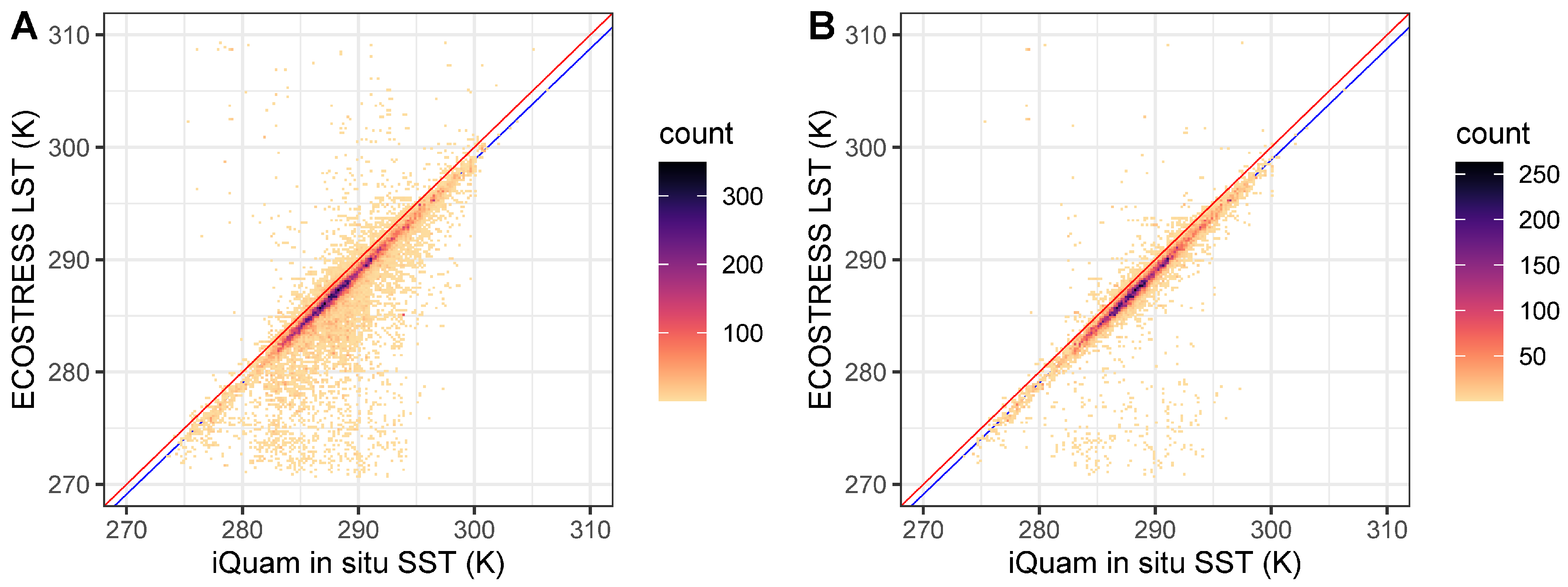
3.1. Matchups
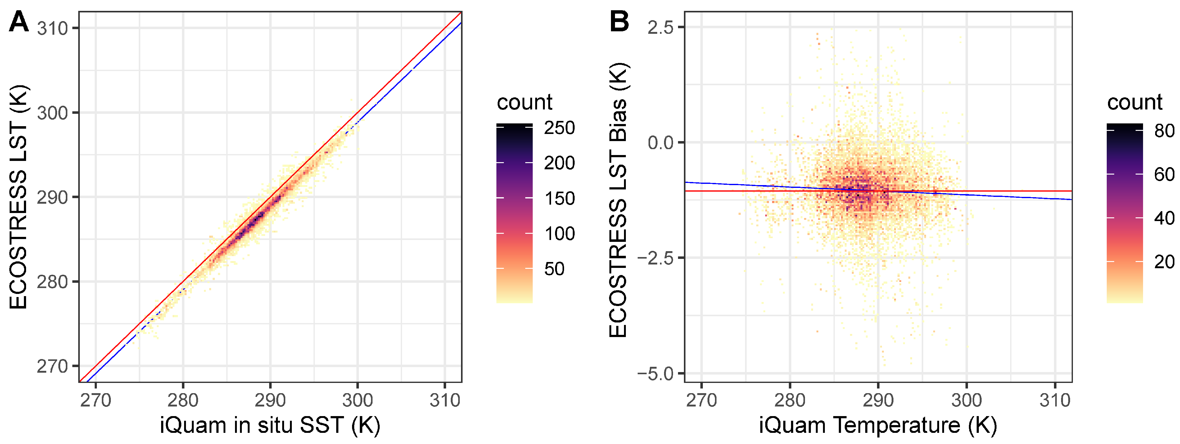
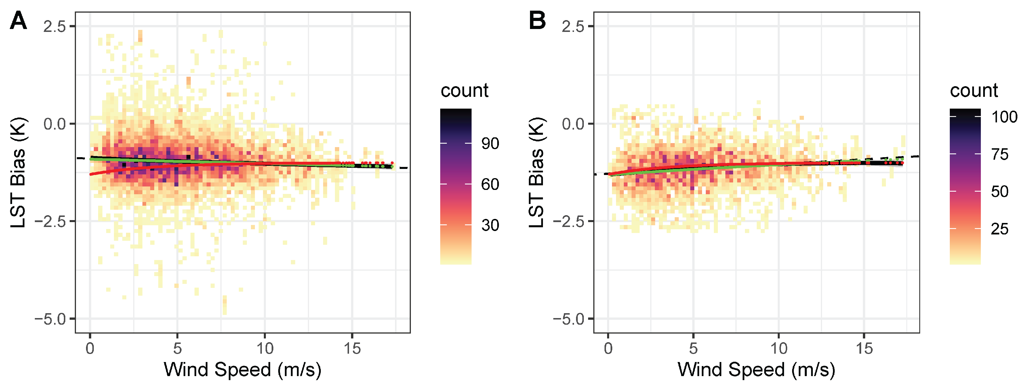
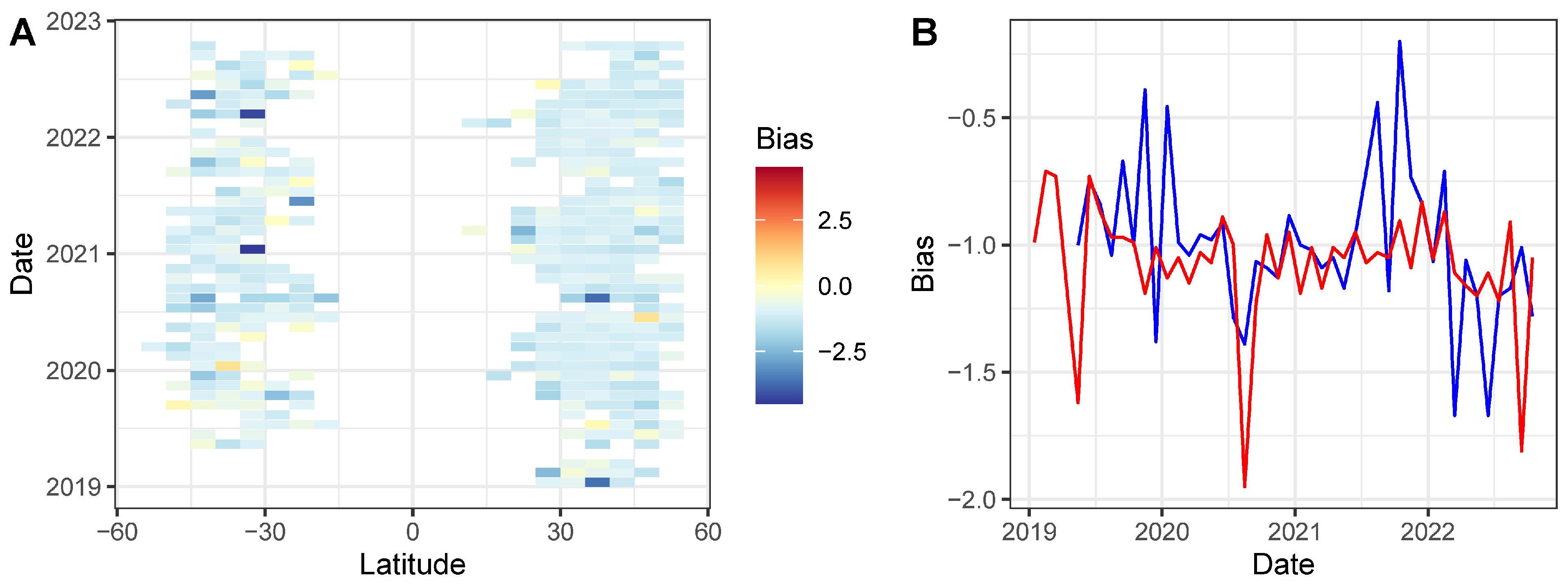
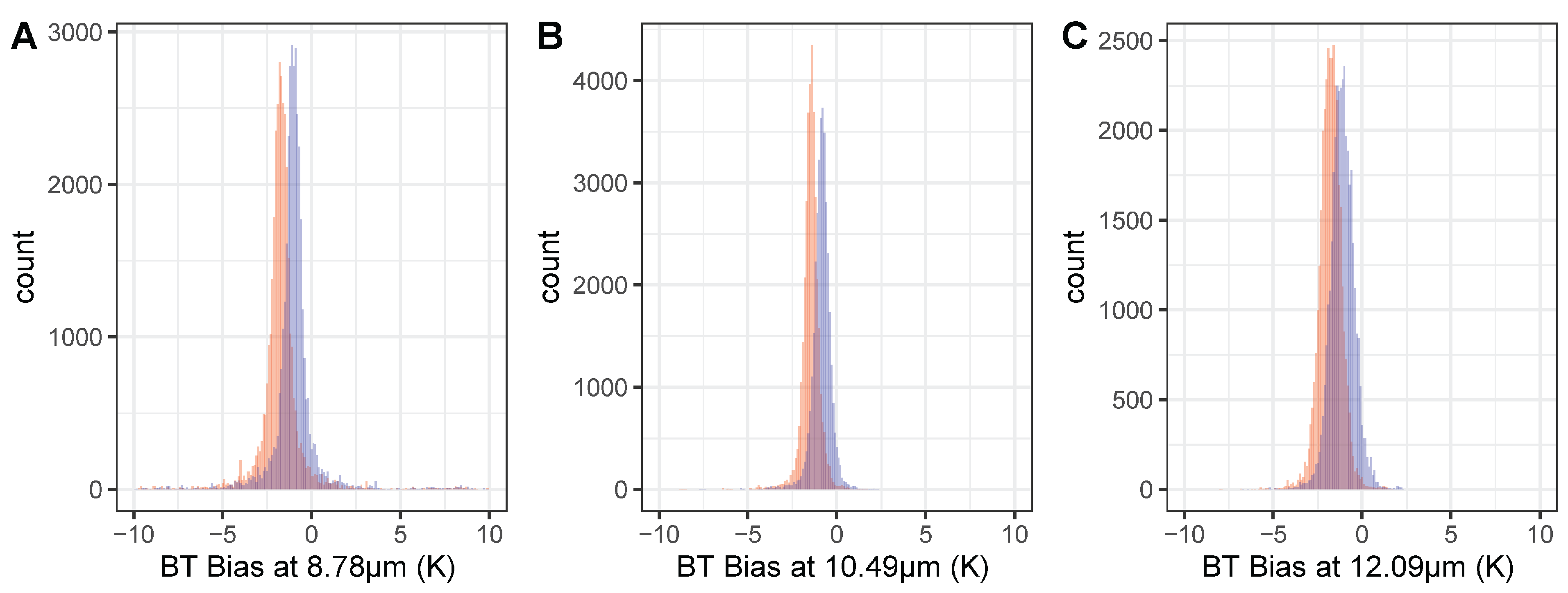
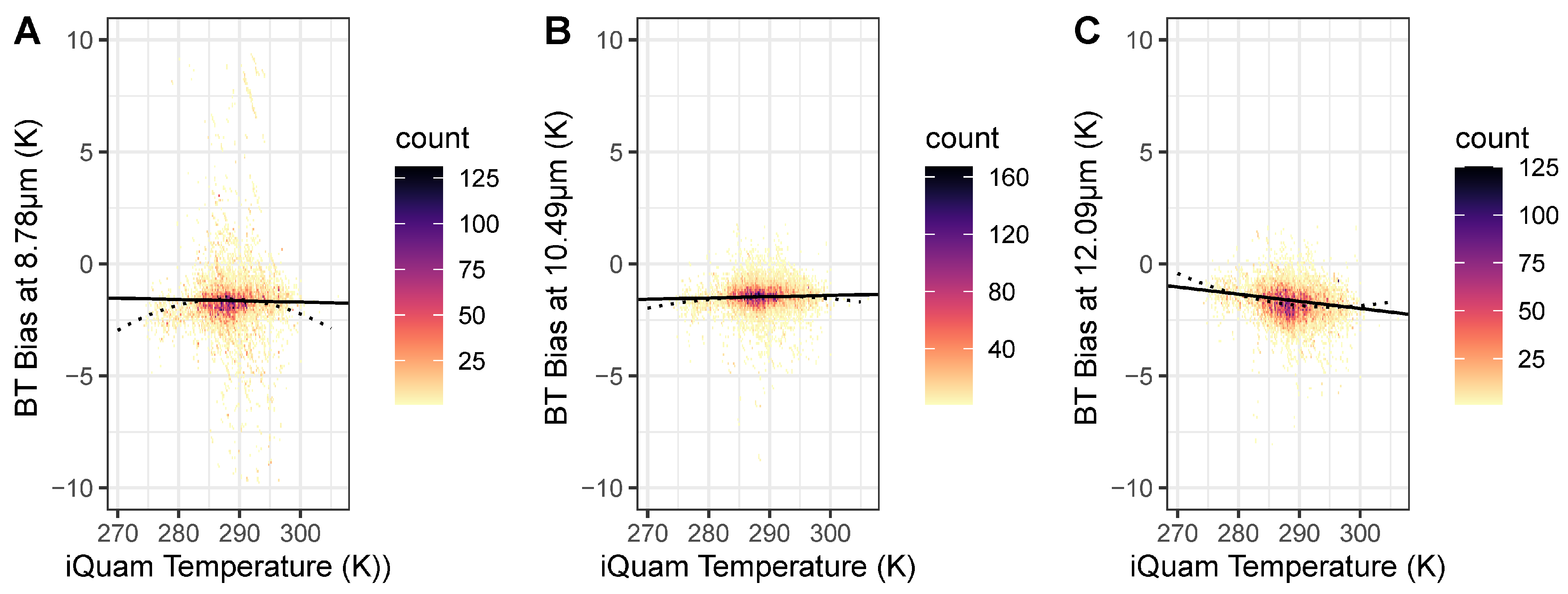
3.2. Bias Analysis
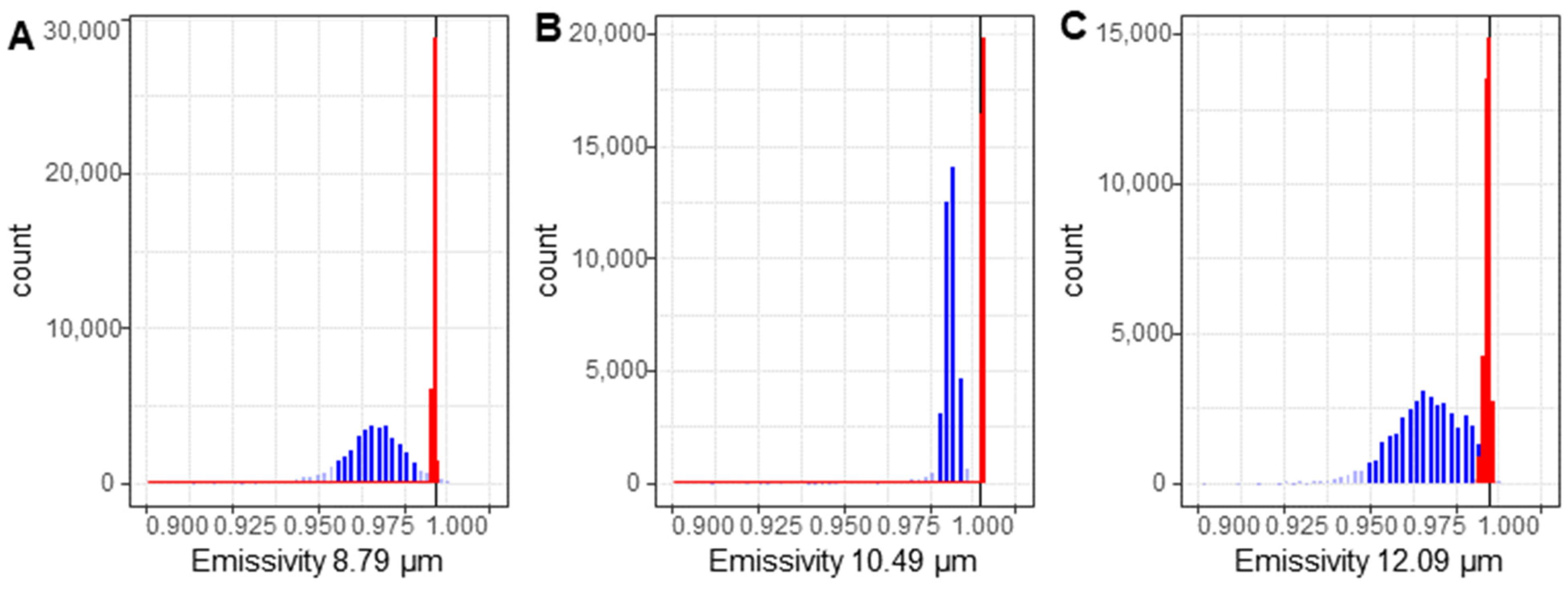
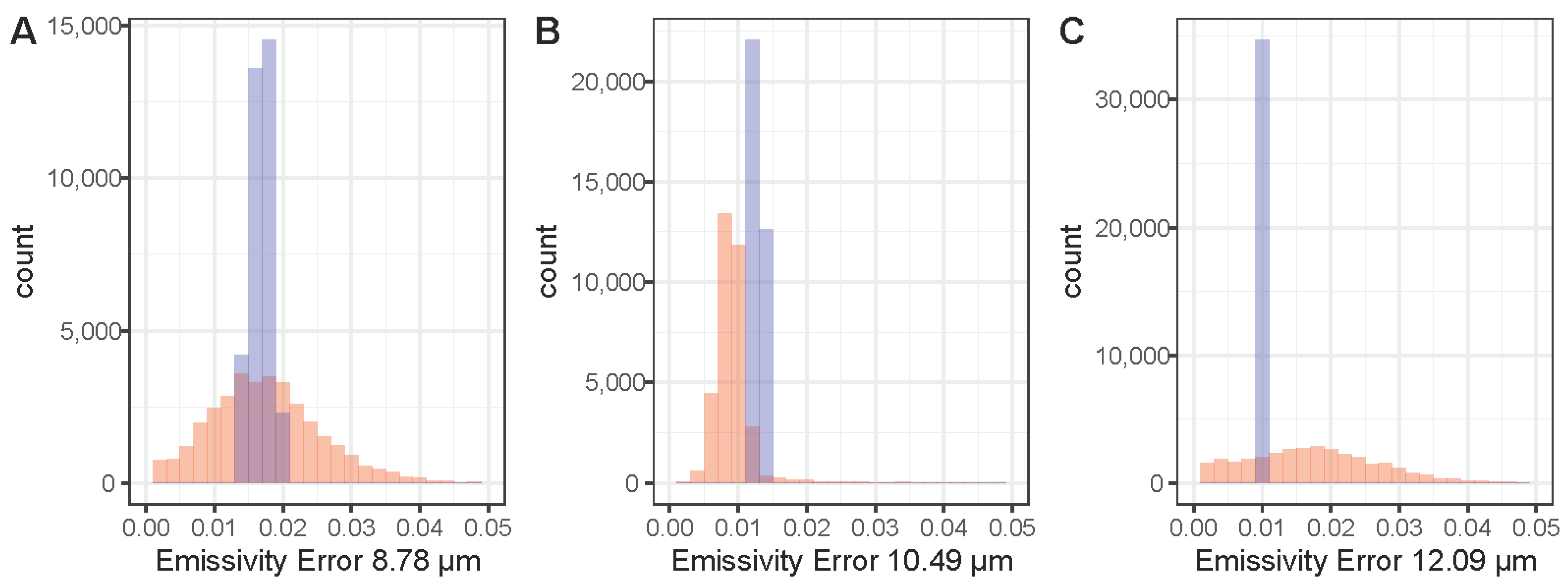
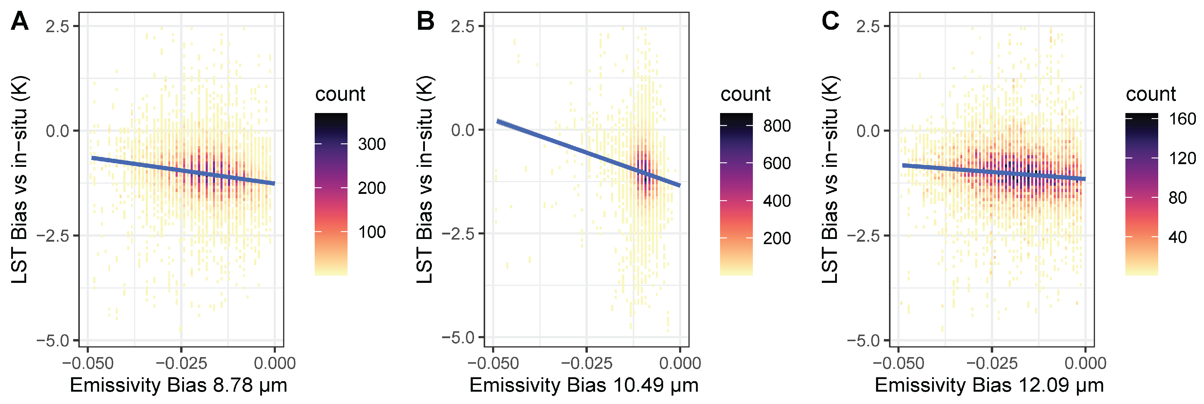
3.3. Emissivity Bias
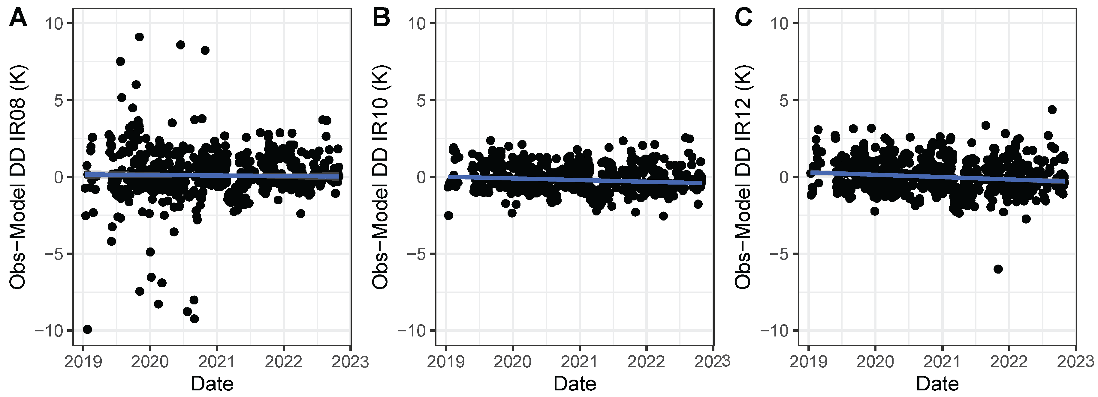
3.4. Sensor Stability
3.5. Focal Plane Detector Radiometric Noise (Temporal Noise)
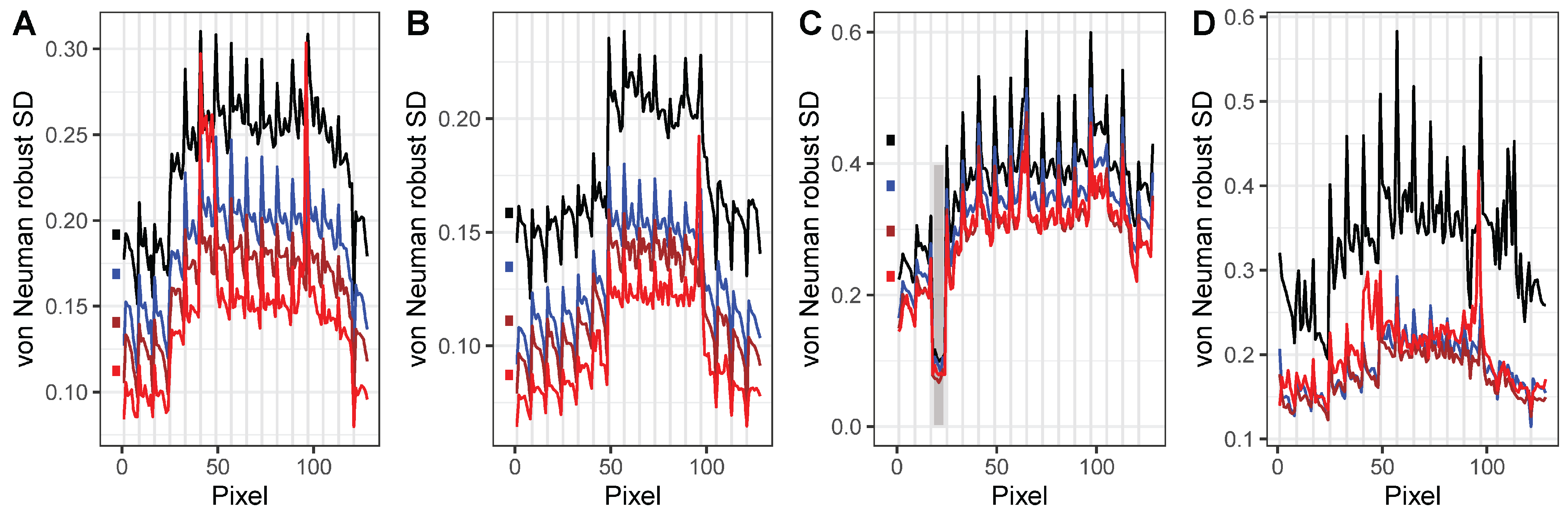
3.6. Focal Plane Non-Uniformity (Spatial Noise)
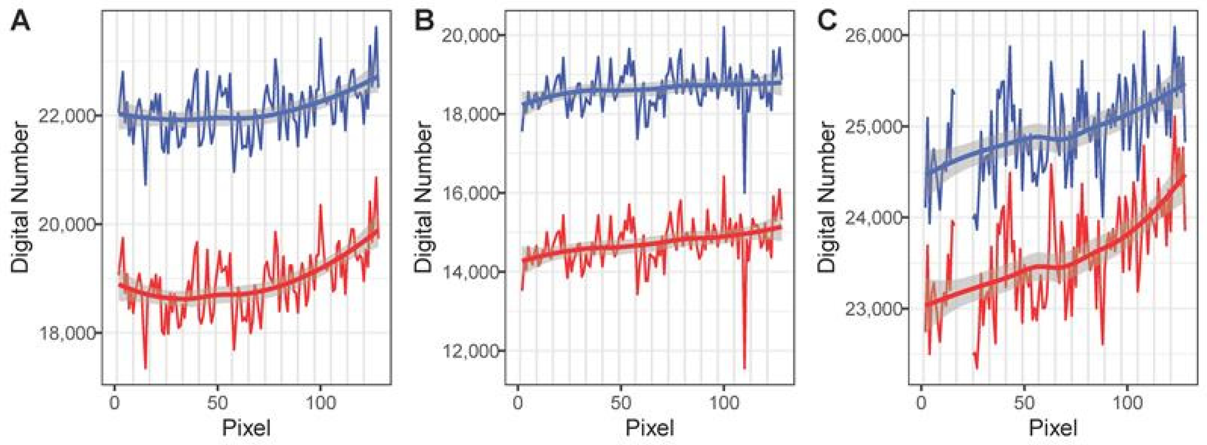
3.7. Black Body Performance
4. Discussion
4.1. Biases
4.2. Radiometric Noise (Temporal and Spatial Noise)
4.3. Black Body Performance
4.4. Radiometric Uncertainty
5. Conclusions
Author Contributions
Funding
Data Availability Statement
Acknowledgments
Conflicts of Interest
Appendix A
References
- Ohring, G.; Wielicki, B.; Spencer, R.; Emery, B.; Datla, R. Satellite Instrument Calibration For Measuring Global Climate Change—Workshop Report. Bull. Am. Meteorol. Soc. 2005, 86, 1303–1314. [Google Scholar] [CrossRef]
- Minnett, P.J.; Alvera-Azcárate, A.; Chin, T.M.; Corlett, G.K.; Gentemann, C.L.; Karagali, I.; Li, X.; Marsouin, A.; Marullo, S.; Maturi, E.; et al. Half a Century of Satellite Remote Sensing of Sea-Surface Temperature. Remote Sens. Environ. 2019, 233, 111366. [Google Scholar] [CrossRef]
- O’Carroll, A.G.; Armstrong, E.M.; Beggs, H.M.; Bouali, M.; Casey, K.S.; Corlett, G.K.; Dash, P.; Donlon, C.J.; Gentemann, C.L.; Høyer, J.L.; et al. Observational Needs of Sea Surface Temperature. Front. Mar. Sci. 2019, 6, 420. [Google Scholar] [CrossRef]
- Merchant, C.J.; Embury, O.; Bulgin, C.E.; Block, T.; Corlett, G.K.; Fiedler, E.; Good, S.A.; Mittaz, J.; Rayner, N.A.; Berry, D.; et al. Satellite-Based Time-Series of Sea-Surface Temperature since 1981 for Climate Applications. Sci. Data 2019, 6, 223. [Google Scholar] [CrossRef] [PubMed]
- Dash, P.; Ignatov, A.; Kihai, Y.; Sapper, J. The SST Quality Monitor (SQUAM). J. Atmos. Ocean. Technol. 2010, 27, 1899–1917. [Google Scholar] [CrossRef]
- Hook, S.; Smyth, M.; Logan, T.; Johnson, W. ECOSTRESS Geolocation Daily L1B Global 70 m V001 [Data Set]. Available online: https://doi.org/10.5067/ECOSTRESS/ECO1BGEO.001 (accessed on 17 March 2024).
- Hook, S.; Smyth, M.; Logan, T.; Johnson, W. ECOSTRESS At-Sensor Calibrated Radiance Daily L1B Global 70 m V001. Available online: https://doi.org/10.5067/ECOSTRESS/ECO1BRAD.001 (accessed on 17 March 2024).
- Hook, S.; Hulley, G. ECOSTRESS Land Surface Temperature and Emissivity Daily L2 Global 70 m V001. Available online: https://doi.org/10.5067/ECOSTRESS/ECO2LSTE.001 (accessed on 23 March 2024).
- Hook, S.; Hulley, G. ECOSTRESS Cloud Mask Daily L2 Global 70 m V001. Available online: https://doi.org/10.5067/ECOSTRESS/ECO2CLD.001 (accessed on 17 March 2024).
- Hulley, G.C.; Hook, S.J. ECOSTRESS Level-2 Land Surface Temperature and Emissivity Algorithm Theoretical Basis Document (ATBD); Jet Propulsion Laboratory: Pasadena, CA, USA, 2016. Available online: https://lpdaac.usgs.gov/documents/1324/ECO2_LSTE_ATBD_V1.pdf (accessed on 22 May 2024).
- Gillespie, A.; Rokugawa, S.; Matsunaga, T.; Cothern, J.S.; Hook, S.; Kahle, A.B. A Temperature and Emissivity Separation Algorithm for Advanced Spaceborne Thermal Emission and Reflection Radiometer (ASTER) Images. IEEE Trans. Geosci. Remote Sens. 1998, 36, 1113–1126. [Google Scholar] [CrossRef]
- Petrenko, B.; Ignatov, A.; Kihai, Y.; Stroup, J.; Dash, P. Evaluation and Selection of SST Regression Algorithms for JPSS VIIRS. JGR Atmos. 2014, 119, 4580–4599. [Google Scholar] [CrossRef]
- Merchant, C.J.; Harris, A.R.; Maturi, E.; Embury, O.; MacCallum, S.N.; Mittaz, J.; Old, C.P. Sea Surface Temperature Estimation from the Geostationary Operational Environmental Satellite-12 (GOES-12). J. Atmos. Ocean. Technol. 2009, 26, 570–581. [Google Scholar] [CrossRef]
- Watts, P.D.; Allen, M.R.; Nightingale, T.J. Wind Speed Effects on Sea Surface Emission and Reflection for the Along Track Scanning Radiometer. J. Atmos. Ocean. Technol. 1996, 13, 126–141. [Google Scholar] [CrossRef]
- Masuda, K. Infrared Sea Surface Emissivity Including Multiple Reflection Effect for Isotropic Gaussian Slope Distribution Model. Remote Sens. Environ. 2006, 103, 488–496. [Google Scholar] [CrossRef]
- Newman, S.M.; Smith, J.A.; Glew, M.D.; Rogers, S.M.; Taylor, J.P. Temperature and Salinity Dependence of Sea Surface Emissivity in the Thermal Infrared. Q. J. R. Meteorol. Soc. 2005, 131, 2539–2557. [Google Scholar] [CrossRef]
- Hocking, J.; Rayer, P.; Rundle, D.; Saunders, R.; Matricardi, M.; Geer, A.; Brunel, P.; Vidot, J. RTTOV V12 Users Guide; Eumetsat NWP SAF: Reading, UK, 2019; Available online: https://nwp-saf.eumetsat.int/site/download/documentation/rtm/docs_rttov12/users_guide_rttov12_v1.3.pdf (accessed on 22 May 2024).
- Gladkova, I.; Ignatov, A.; Semenov, A. Analaysis of ABI Bands and Regressors in the ACSPO GEO NLSST Algorithm. In Proceedings of the SPIE Defense + Commercial Sensing, Orlando, FL, USA, 3–7 April 2022; SPIE: Bellingham, WA, USA, 2022; Volume 12118, p. 1211804. [Google Scholar] [CrossRef]
- Saux Picart, S. Algorithms Theoretical Basis Document for Low Earth Orbiter Sea Surface Temperature Processing; Eumetsat OSI SAF: Lannion, France, 2018; Available online: https://osi-saf.eumetsat.int/lml/doc/osisaf_cdop2_ss1_atbd_leo_sst.pdf (accessed on 22 May 2024).
- Hook, S.J.; Cawse-Nicholson, K.; Barsi, J.; Radocinski, R.; Hulley, G.C.; Johnson, W.R.; Rivera, G.; Markham, B. In-Flight Validation of the ECOSTRESS, Landsats 7 and 8 Thermal Infrared Spectral Channels Using the Lake Tahoe CA/NV and Salton Sea CA Automated Validation Sites. IEEE Trans. Geosci. Remote Sens. 2020, 58, 1294–1302. [Google Scholar] [CrossRef]
- Hulley, G.C.; Gottsche, F.M.; Rivera, G.; Hook, S.J.; Freepartner, R.J.; Martin, M.A.; Cawse-Nicholson, K.; Johnson, W.R. Validation and Quality Assessment of the ECOSTRESS Level-2 Land Surface Temperature and Emissivity Product. IEEE Trans. Geosci. Remote Sens. 2022, 60, 1–23. [Google Scholar] [CrossRef]
- Shi, J.; Hu, C. Evaluation of ECOSTRESS Thermal Data over South Florida Estuaries. Sensors 2021, 21, 4341. [Google Scholar] [CrossRef] [PubMed]
- Weidberg, N.; Wethey, D.S.; Woodin, S.A. Global Intercomparison of Hyper-Resolution ECOSTRESS Coastal Sea Surface Temperature Measurements from the Space Station with VIIRS-N20. Remote Sens. 2021, 13, 5021. [Google Scholar] [CrossRef]
- Xu, F.; Ignatov, A. In Situ SST Quality Monitor (iQuam). J. Atmos. Ocean. Technol. 2014, 31, 164–180. [Google Scholar] [CrossRef]
- NOAA/NESDIS/STAR GHRSST L2P ACSPO America Region SST from GOES-16 ABI. Available online: https://doi.org/10.5067/GHG16-2PO27 (accessed on 23 March 2024).
- NOAA/NESDIS/STAR GHRSST L2P ACSPO America Region SST from GOES-17 ABI. Available online: https://doi.org/10.5067/GHG17-2PO71 (accessed on 23 March 2024).
- NOAA/NESDIS/STAR GHRSST NOAA/STAR Himawari-08 AHI L2P Pacific Ocean Region SST v2.70 Dataset in GDS2. Available online: https://doi.org/10.5067/GHH08-2PO27 (accessed on 23 March 2024).
- NOAA/NESDIS/OSPO GHRSST Level 2P Indian Ocean Regional Skin Sea Surface Temperature v1.0 from the Spinning Enhanced Visible and InfraRed Imager (SEVIRI) on the Meteosat Second Generation-1 (MSG-1) Satellite. Available online: https://doi.org/10.5067/GHMG1-2PO01 (accessed on 17 March 2024).
- NOAA/NESDIS/OSPO NOAA GHRSST Level 2P Indian Ocean Regional Skin Sea Surface Temperature v1.0 from the Spinning Enhanced Visible and InfraRed Imager (SEVIRI) on the Meteosat Second Generation-2 (MSG-2) Satellite. Available online: https://doi.org/10.5067/GHMG2-2PO10 (accessed on 17 March 2024).
- NOAA/NESDIS/OSPO NOAA GHRSST Level 2P Atlantic Ocean Regional Skin Sea Surface Temperature v1.0 from the Spinning Enhanced Visible and InfraRed Imager (SEVIRI) on the Meteosat Second Generation-4 (MSG-4) Satellite. Available online: https://doi.org/10.5067/GHMG4-2PO01 (accessed on 23 March 2024).
- Masuda, K.; Takashima, T.; Takayama, Y. Emissivity of Pure and Sea Waters for the Model Sea Surface in the Infrared Window Regions. Remote Sens. Environ. 1988, 24, 313–329. [Google Scholar] [CrossRef]
- Masuda, K. Dependence of Sea Surface Emissivity on Temperature-dependent Refractive Index. Q. J. R. Meteorol. Soc. 2008, 134, 541–545. [Google Scholar] [CrossRef]
- NOAA/NESDIS/OSPO NOAA GHRSST Level 2P Atlantic Ocean Regional Skin Sea Surface Temperature v1.0 from the Spinning Enhanced Visible and InfraRed Imager (SEVIRI) on the Meteosat Second Generation-3 (MSG-3) Satellite. Available online: https://doi.org/10.5067/GHMG3-2PO02 (accessed on 23 March 2024).
- Minnett, P.J.; Smith, M.; Ward, B. Measurements of the Oceanic Thermal Skin Effect. Deep. Sea Res. Part II Top. Stud. Oceanogr. 2011, 58, 861–868. [Google Scholar] [CrossRef]
- Hulley, G.C.; Hook, S.J. ECOSTRESS Level-2 Cloud Detection Algorithm Theoretical Basis Document (ATBD); Jet Propulsion Laboratory: Pasadena, CA, USA, 2018. Available online: https://lpdaac.usgs.gov/documents/296/ECO2_Cloud_ATBD_V1.pdf (accessed on 22 May 2024).
- Walton, C.C.; Sullivan, J.T.; Rao, C.R.N.; Weinreb, M.P. Corrections for Detector Nonlinearities and Calibration Inconsistencies of the Infrared Channels of the Advanced Very High Resolution Radiometer. J. Geophys. Res. 1998, 103, 3323–3337. [Google Scholar] [CrossRef]
- Theocharous, E.; Ishii, J.; Fox, N.P. Absolute Linearity Measurements on HgCdTe Detectors in the Infrared Region. Appl. Opt. 2004, 43, 4182. [Google Scholar] [CrossRef] [PubMed]
- Theocharous, E.; Theocharous, O.J. Practical Limit of the Accuracy of Radiometric Measurements Using HgCdTe Detectors. Appl. Opt. 2006, 45, 7753. [Google Scholar] [CrossRef] [PubMed]
- Arai, K.; Tonooka, H. Radiometric Performance Evaluation of ASTER VNIR, SWIR, and TIR. IEEE Trans. Geosci. Remote Sens. 2005, 43, 2725–2732. [Google Scholar] [CrossRef]
- Mittaz, J.P.D.; Harris, A.R.; Sullivan, J.T. A Physical Method for the Calibration of the AVHRR/3 Thermal IR Channels 1: The Prelaunch Calibration Data. J. Atmos. Ocean. Technol. 2009, 26, 996–1019. [Google Scholar] [CrossRef]
- Mittaz, J.; Harris, A. A Physical Method for the Calibration of the AVHRR/3 Thermal IR Channels. Part II: An In-Orbit Comparison of the AVHRR Longwave Thermal IR Channels on Board MetOp-A with IASI. J. Atmos. Ocean. Technol. 2011, 28, 1072–1087. [Google Scholar] [CrossRef]
- Chang, T.; Wu, X.; Weng, F. Modeling Thermal Emissive Bands Radiometric Calibration Impact with Reference to AVHRR. J. Geophys. Res. Atmos. 2017, 122, 2831–2843. [Google Scholar] [CrossRef]
- Sakuma, F.; Ono, A.; Tsuchida, S.; Ohgi, N.; Inada, H.; Akagi, S.; Ono, H. Onboard Calibration of the ASTER Instrument. IEEE Trans. Geosci. Remote Sens. 2005, 43, 2715–2724. [Google Scholar] [CrossRef]
- Tonooka, H.; Sakuma, F.; Tachikawa, T.; Kikuchi, M. Radiometric Calibration Status and Recalibration of Aster Thermal Infrared Images. In Proceedings of the IGARSS 2019—2019 IEEE International Geoscience and Remote Sensing Symposium, Yokohama, Japan, 28 July–2 August 2019; IEEE: New York, NY, USA, 2019; pp. 8530–8533. [Google Scholar] [CrossRef]
- Smith, D.; Barillot, M.; Bianchi, S.; Brandani, F.; Coppo, P.; Etxaluze, M.; Frerick, J.; Kirschstein, S.; Lee, A.; Maddison, B.; et al. Sentinel-3A/B SLSTR Pre-Launch Calibration of the Thermal InfraRed Channels. Remote Sens. 2020, 12, 2510. [Google Scholar] [CrossRef]
- Xiong, X.; Butler, J.J. MODIS and VIIRS Calibration History and Future Outlook. Remote Sens. 2020, 12, 2523. [Google Scholar] [CrossRef]
- Cao, C.; Wang, W.; Blonski, S.; Zhang, B. Radiometric Traceability Diagnosis and Bias Correction for the Suomi NPP VIIRS Long-wave Infrared Channels during Blackbody Unsteady States. JGR Atmos. 2017, 122, 5285–5297. [Google Scholar] [CrossRef]
- Efremova, B.; McIntire, J.; Moyer, D.; Wu, A.; Xiong, X. S-NPP VIIRS Thermal Emissive Bands on-Orbit Calibration and Performance. J. Geophys. Res. Atmos. 2014, 119, 10859–10875. [Google Scholar] [CrossRef]
- Pérez Díaz, C.L.; Xiong, X.; Li, Y.; Chiang, K. S-NPP VIIRS Thermal Emissive Bands 10-Year On-Orbit Calibration and Performance. Remote Sens. 2021, 13, 3917. [Google Scholar] [CrossRef]
- Logan, T.L.; Johnson, W.R. ECOSTRESS Level-1 Focal Plane Array and Radiometric Calibration Algorithm Theoretical Basis Document; Jet Propulsion Laboratory: Pasadena, CA, USA, 2018. Available online: https://lpdaac.usgs.gov/documents/222/ECO1B_Calibration_ATBD_V1.pdf (accessed on 22 May 2024).
- Johnson, W.R.; Hook, S.J.; Schmitigal, W.; Goullioud, R. ECOSTRESS End-to-End Radiometric Pre-Flight Calibration and Validation. In Proceedings of the SPIE Optical Engineering + Applications, San Diego, CA, USA, 19–23 August 2018. [Google Scholar] [CrossRef]
- Smyth, M.M.; Logan, T.L. ECOSTRESS Level 1 Product User Guide Version 3; Jet Propulsion Laboratory: Pasadena, CA, USA, 2022. Available online: https://lpdaac.usgs.gov/documents/1491/ECO1B_User_Guide_V2.pdf (accessed on 22 May 2024).
- Johnson, W. ECOSTRESS Lab Performance. In Proceedings of the HyspIRI Workshop, Pasadena, CA, USA, 19 October 2016; Available online: https://hyspiri.jpl.nasa.gov/downloads/2016_Workshop/day2/14_161019-ECOSTRESS_Lab_Performance_3.pdf (accessed on 22 May 2024).
- Smyth, M.; Leprince, S. ECOSTRESS Level-1B Resampling and Geolocation Algorithm Theoretical Basis Document (ATBD); Jet Propulsion Laboratory: Pasadena, CA, USA, 2018. Available online: https://lpdaac.usgs.gov/223/ECO1B_Geolocation_ATBD_V1.pdf (accessed on 22 May 2024).
- Krehbiel, K. ECOSTRESS Swath to Grid Conversion Script. Available online: https://git.earthdata.nasa.gov/projects/LPDUR/repos/ecostress_swath2grid/browse (accessed on 17 March 2024).
- Buffet, L.; Gamet, P.; Maisongrande, P.; Salcedo, C.; Crebassol, P. The TIR Instrument on TRISHNA Satellite: A Precursor of High Resolution Observation Missions in the Thermal Infrared Domain. In Proceedings of the International Conference on Space Optics—ICSO 2020, Virtual Conference, 30 March–2 April 2021; Cugny, B., Sodnik, Z., Karafolas, N., Eds.; SPIE: Bellingham, WA, USA, 2021; p. 118520. Available online: https://www.spiedigitallibrary.org/conference-proceedings-of-spie/11852/2599173/The-TIR-instrument-on-TRISHNA-satellite--a-precursor-of/10.1117/12.2599173.full (accessed on 22 May 2024).
- Cawse-Nicholson, K.; Townsend, P.A.; Schimel, D.; Assiri, A.M.; Blake, P.L.; Buongiorno, M.F.; Campbell, P.; Carmon, N.; Casey, K.A.; Correa-Pabón, R.E.; et al. NASA’s Surface Biology and Geology Designated Observable: A Perspective on Surface Imaging Algorithms. Remote Sens. Environ. 2021, 257, 112349. [Google Scholar] [CrossRef]
- Koetz, B.; Bastiaanssen, W.; Berger, M.; Defourney, P.; Del Bello, U.; Drusch, M.; Drinkwater, M.; Duca, R.; Fernandez, V.; Ghent, D.; et al. High Spatio-Temporal Resolution Land Surface Temperature Mission—A Copernicus Candidate Mission in Support of Agricultural Monitoring. In Proceedings of the IGARSS 2018—2018 IEEE International Geoscience and Remote Sensing Symposium, Valencia, Spain, 22–27 July 2018; IEEE: Bellingham, WA, USA, 2018; pp. 8160–8162. [Google Scholar] [CrossRef]
- Xu, F.; Ignatov, A. Error Characterization in iQuam SSTs Using Triple Collocations with Satellite Measurements. Geophys. Res. Lett. 2016, 43, 10826–10834. [Google Scholar] [CrossRef]
- Xu, F.; Ignatov, A. iQuam In Situ SST Quality Monitor v2.10. Available online: https://www.star.nesdis.noaa.gov/socd/sst/iquam/data.html (accessed on 18 March 2024).
- LPDAAC ECOSTRESS Brightness Temperature Lookup Tables. Available online: https://git.earthdata.nasa.gov/projects/LPDUR/repos/ecostress_swath2grid/browse/EcostressBrightnessTemperatureV01.h5 (accessed on 17 March 2024).
- European Centre for Medium-Range Weather Forecasts ERA5 Reanalysis (0.25 Degree Latitude-Longitude Grid). Available online: https://doi.org/10.5065/BH6N-5N20 (accessed on 17 March 2024).
- Saunders, R.; Hocking, J.; Rundle, D.; Rayer, P.; Havemann, S.; Matricardi, M.; Geer, A.; Lupu, C.; Brunel, P.; Vidot, J. RTTOV-12 Science and Validation Report; Eumetsat NWP SAF: Reading, UK, 2017; Available online: https://nwp-saf.eumetsat.int/site/download/documentation/rtm/docs_rttov12/rttov12_svr.pdf (accessed on 22 May 2024).
- Donlon, C.J.; Minnett, P.J.; Gentemann, C.; Nightingale, T.J.; Barton, I.J.; Ward, B.; Murray, M.J. Toward Improved Validation of Satellite Sea Surface Skin Temperature Measurements for Climate Research. J. Clim. 2002, 15, 353–369. [Google Scholar] [CrossRef]
- Liang, X.; Ignatov, A. Monitoring of IR Clear-Sky Radiances over Oceans for SST (MICROS). J. Atmos. Ocean. Technol. 2011, 28, 1228–1242. [Google Scholar] [CrossRef]
- Liberti, G.L.; Sabatini, M.; Wethey, D.S.; Ciani, D. A Multi-Pixel Split-Window Approach to Sea Surface Temperature Retrieval from Thermal Imagers with Relatively High Radiometric Noise: Preliminary Studies. Remote Sens. 2023, 15, 2453. [Google Scholar] [CrossRef]
- Von Neumann, J. Distribution of the Ratio of the Mean Square Successive Difference to the Variance. Ann. Math. Statist. 1941, 12, 367–395. [Google Scholar] [CrossRef]
- R Core Team. R: A Language and Environment for Statistical Computing. Available online: https://www.R-project.org (accessed on 22 May 2024).
- RStudio Team. RStudio: Integrated Development for R. Available online: https://www.posit.co (accessed on 22 May 2024).
- Pierce, D. Ncdf4: Interface to Unidata netCDF (Version 4 or Earlier) Format Data. Available online: https://CRAN.R-project.org/package=ncdf4 (accessed on 23 March 2024).
- Fischer, B.; Smith, M.; Pau, G. Rhdf5: R Interface to HDF5. Available online: https://doi.org/10.18129/B9.bioc.rhdf5 (accessed on 22 May 2024).
- Ooms, J. Sys: Powerful and Reliable Tools for Running System Commands in R. Available online: https://CRAN.R-project.org/package=sys (accessed on 23 March 2024).
- Schmidt, D.; Chen, W. getPass: Masked User Input. Available online: https://cran.r-project.org/package=getPass (accessed on 22 May 2024).
- Wickham, H. Httr: Tools for Working with Urls and Http. Available online: https://CRAN.R-project.org/package=httr (accessed on 23 March 2023).
- Wickham, H.; Henry, L. Purrr: Functional Programming Tools. Available online: https://CRAN.R-project.org/package=purrr (accessed on 23 March 2024).
- Wickham, H. Rvest: Easily Harvest (Scrape) Web Pages. Available online: https://CRAN.R-project.org/package=rvest (accessed on 23 March 2024).
- Wickham, H.; François, R.; Henry, L.; Müller, K.; Vaughan, D. Dplyr: A Grammar of Data Manipulation. Available online: https://CRAN.R-project.org/package=dplyr (accessed on 23 March 2024).
- Plate, T.; Heiberger, R. Abind: Combine Multidimensional Arrays. Available online: https://CRAN.R-project.org/package=abind (accessed on 23 March 2024).
- Hiebert, J. Udunits2: Udunits-2 Bindings for R. Available online: https://CRAN.R-project.org/package=udunits2 (accessed on 22 May 2024).
- Lai, R. Retry: Repeated Evaluation. Available online: https://CRAN.R-project.org/package=retry (accessed on 23 March 2024).
- Hijmans, R.J. Terra: Spatial Data Analysis. Available online: https://CRAN.R-project.org/package=terra (accessed on 23 March 2024).
- Arya, S.; Mount, D.; Kemp, S.E.; Jefferis, G. RANN: Fast Nearest Neighbour Search (Wraps ANN Library) Using L2 Metric. Available online: https://CRAN.R-project.org/package=RANN (accessed on 23 March 2024).
- Pebesma, E.; Bivand, R. Sp: Classes and Methods for Spatial Data in R. Available online: https://CRAN.R-project.org/package=sp (accessed on 23 March 2024).
- Baddeley, A.; Rubak, E.; Turner, R. Spatstat: An R Package for Analyzing Spatial Point Patterns. Available online: https://CRAN.R-project.org/package=spatstat (accessed on 23 March 2024).
- Dutky, S.; Maechler, M. Bitops: Bitwise Operations. Available online: https://CRAN.R-project.org/package=bitops (accessed on 23 March 2024).
- Chau, J. Gslnls: GSL Nonlinear Least Squares Fitting. Available online: https://CRAN.R-project.org/package=gslnls (accessed on 23 March 2024).
- Pierre-Jean, M.; Gigaill, G.; Neuvial, P. Jointseg: Joint Segmentation of Multivariate (Copy Number) Signals. Available online: https://CRAN.R-project.org/package=jointseg (accessed on 23 March 2024).
- Signorell, A. DescTools: Tools for Descriptive Statistics. Available online: https://CRAN.R-project.org/package=DescTools (accessed on 23 March 2024).
- Wickham, H. Ggplot2: Elegant Graphics for Data Analysis. Available online: https://ggplot2.tidyverse.org (accessed on 23 March 2024).
- Garnier, S.; Ross, N.; Rudis, R.; Camargo, A.P.; Sciaini, M.; Scherer, C. Viridis: Colorblind-Friendly Color Maps for R. Available online: https://cran.r-project.org/package=viridis (accessed on 23 March 2024).
- Kassambara, A. Ggpubr: “ggplot2” Based Publication Ready Plots. Available online: https://CRAN.R-project.org/package=ggpubr (accessed on 23 March 2024).
- NOAA SST Quality Monitor. Available online: https://www.star.nesdis.noaa.gov/socd/sst/squam/index.php (accessed on 5 April 2024).
- Baldridge, A.M.; Hook, S.J.; Grove, C.I.; Rivera, G. The ASTER Spectral Library Version 2.0. Remote Sens. Environ. 2009, 113, 711–715. [Google Scholar] [CrossRef]
- Padula, F.; Cao, C. Detector-Level Spectral Characterization of the Suomi National Polar-Orbiting Partnership Visible Infrared Imaging Radiometer Suite Long-Wave Infrared Bands M15 and M16. Appl. Opt. 2015, 54, 5109. [Google Scholar] [CrossRef] [PubMed]
- Wang, Z.; Cao, C. Assessing the Effects of Suomi NPP VIIRS M15/M16 Detector Radiometric Stability and Relative Spectral Response Variation on Striping. Remote Sens. 2016, 8, 145. [Google Scholar] [CrossRef]
- Oudrari, H.; McIntire, J.; Xiong, X.; Butler, J.; Ji, Q.; Schwarting, T.; Lee, S.; Efremova, B. JPSS-1 VIIRS Radiometric Characterization and Calibration Based on Pre-Launch Testing. Remote Sens. 2016, 8, 41. [Google Scholar] [CrossRef]
- Lin, L.; Cao, C. The Effects of VIIRS Detector-Level and Band-Averaged Relative Spectral Response Differences Between S-NPP and NOAA-20 on the Thermal Emissive Bands. IEEE J. Sel. Top. Appl. Earth Obs. Remote Sens. 2019, 12, 4123–4130. [Google Scholar] [CrossRef]
- Jau, B.M.; Hook, S.J.; Johnson, W.R.; Foote, M.C.; Paine, C.G.; Pannell, Z.W.; Smythe, R.F.; Kuan, G.M.; Jablonski, J.K.; Eng, B.T. PHyTIR-A Prototype Thermal Infrared Radiometer; IEEE: Big Sky, MT, USA, 2013; Available online: https://hdl.handle.net/2014/44954 (accessed on 22 May 2024).
- Wang, W.; Cao, C. NOAA-20 and S-NPP VIIRS Thermal Emissive Bands On-Orbit Calibration Algorithm Update and Long-Term Performance Inter-Comparison. Remote Sens. 2021, 13, 448. [Google Scholar] [CrossRef]
- Smith, D.; Hunt, S.E.; Etxaluze, M.; Peters, D.; Nightingale, T.; Mittaz, J.; Woolliams, E.R.; Polehampton, E. Traceability of the Sentinel-3 SLSTR Level-1 Infrared Radiometric Processing. Remote Sens. 2021, 13, 374. [Google Scholar] [CrossRef]
- Madhavan, S.; Xiong, X.; Wu, A.; Wenny, B.N.; Chiang, K.; Chen, N.; Wang, Z.; Li, Y. Noise Characterization and Performance of MODIS Thermal Emissive Bands. IEEE Trans. Geosci. Remote Sens. 2016, 54, 3221–3234. [Google Scholar] [CrossRef] [PubMed]
- Bouali, M.; Ignatov, A. Estimation of Detector Biases in MODIS Thermal Emissive Bands. IEEE Trans. Geosci. Remote Sens. 2013, 51, 4339–4348. [Google Scholar] [CrossRef]
- Charvet, D.; Gnata, X.; Toulemont, A.; Rizzolo, S.; Clénet, A.; Libouban, C.; Gossant, A.; Chassat, F.; Buffet, L.; Salcedo, C.; et al. TRISHNA TIR Instrument Development and Performance Status. In Proceedings of the ICSO 2022, Dubrovnik, Croatia, 3–7 October 2022; SPIE: Bellingham, WA, USA, 2022; Volume 12777, p. 1277742. [Google Scholar] [CrossRef]
- Basilio, R.R.; Hook, S.J.; Zoffoli, S.; Buongiorno, M.F. Surface Biology and Geology (SBG) Thermal Infrared (TIR) Free-Flyer Concept. In Proceedings of the 2022 IEEE Aerospace Conference (AERO), Big Sky, MT, USA, 5–12 March 2022; IEEE: Big Sky, MT, USA, 2022; pp. 1–9. [Google Scholar] [CrossRef]
- Bernard, F.; Bourgeois, G.; Manolis, I.; Barat, I.; Alamanac, A.B.; Taboada, M.S.; Mingorance, P.; Ciapponi, A.; Cardone, T.; Dutruel, E.; et al. The LSTM Instrument: Design, Technology and Performance. In Proceedings of the International Conference on Space Optics—ICSO 2022, Dubrovnik, Croatia, 3–7 October 2022; Minoglou, K., Karafolas, N., Cugny, B., Eds.; SPIE: Bellingham, WA, USA, 2023; p. 144. [Google Scholar] [CrossRef]
- Smith, D.; Mutlow, C.; Delderfield, J.; Watkins, B.; Mason, G. ATSR Infrared Radiometric Calibration and In-Orbit Performance. Remote Sens. Environ. 2012, 116, 4–16. [Google Scholar] [CrossRef]
- Xiong, X.; Wenny, B.N.; Wu, A.; Barnes, W.L. MODIS Onboard Blackbody Function and Performance. IEEE Trans. Geosci. Remote Sens. 2009, 47, 4210–4222. [Google Scholar] [CrossRef]
- Mason, I.M.; Sheather, P.H.; Bowles, J.A.; Davies, G. Blackbody Calibration Sources of High Accuracy for a Spaceborne Infrared Instrument: The Along Track Scanning Radiometer. Appl. Opt. 1996, 35, 629. [Google Scholar] [CrossRef] [PubMed]
- Maple Version 15.01. Available online: https://www.maplesoft.com (accessed on 23 March 2024).

| Scene Number | Orbit_Scene | Date Time (UTC) | Cold BB | Hot BB | ||
|---|---|---|---|---|---|---|
| Mean (K) | sd | Mean (K) | sd | |||
| 1 | 10043_007 | 13 April 2020 14:24:40 | 292.800 | 0.170 | 318.905 | 0.144 |
| 2 | 10072_005 | 15 April 2020 11:13:12 | 293.015 | 0.172 | 318.907 | 0.149 |
| 3 | 10392_001 | 6 May 2020 02:37:16 | 294.086 | 0.178 | 318.918 | 0.145 |
| 4 | 16665_003 | 14 June 2021 10:53:10 | 293.195 | 0.172 | 318.919 | 0.145 |
| 5 | 17169_005 | 16 July 2021 21:47:31 | 292.624 | 0.171 | 318.905 | 0.150 |
| 6 | 17615_009 | 14 August 2021 13:27:20 | 292.868 | 0.169 | 318.912 | 0.143 |
| 7 | 17983_010 | 7 September 2021 04:16:44 | 293.848 | 0.175 | 318.907 | 0.145 |
| Instrument | 8.5 µm | 10–11 µm | 12 µm | |||
|---|---|---|---|---|---|---|
| Noise Type | Spatial | Temporal | Spatial | Temporal | Spatial | Temporal |
| VIIRS | 55 | 25 | 23 | 30 | 39 | |
| SLSTR | 3 | 13 | 3 | 15 | ||
| MODIS | 600 | 30 | 26 | 30 | 32 | 40 |
| ECOSTRESS | 375 | 100–300 | 375 | 60–180 | 625 | 180–520 |
| TRISHNA | 95 | 80 | 70 | 70 | 60 | 70 |
| SBG * | 100 | 100 | 100 | |||
| LSTM * | 100 | 100 | 100 | |||
| Instrument | Hot BB sd (mK) | Cold BB sd (mK) | Source |
|---|---|---|---|
| ATSR | 6.2 | 5.02 | 62 |
| SLSTR-A | 11.6 | 9 | 60 |
| SLSTR-B | 27 | 8 | 63 |
| MODIS-A | 30 | 7 | 64 |
| VIIRS-SNPP | 4 | 59 | |
| VIIRS-N20 | 8 | 59 | |
| ECOSTRESS | 146 | 172 | Table 1 |
| Source of Uncertainty | Uncertainty Estimation | 8.78 µm | 10.49 µm | 12.09 µm |
|---|---|---|---|---|
| NEdT | Figure 11 | 120–250 | 60–180 | 180–520 |
| Cold BB PRT temperatures | 10 | 9.6 | 9.4 | |
| Hot BB PRT temperatures | 11.4 | 10.2 | 9.6 | |
| Focal Plane Non-uniformity | Figure 14 | 125 | 250 | 750 |
| Total | 266–396 | 330–450 | 949–1289 |
Disclaimer/Publisher’s Note: The statements, opinions and data contained in all publications are solely those of the individual author(s) and contributor(s) and not of MDPI and/or the editor(s). MDPI and/or the editor(s) disclaim responsibility for any injury to people or property resulting from any ideas, methods, instructions or products referred to in the content. |
© 2024 by the authors. Licensee MDPI, Basel, Switzerland. This article is an open access article distributed under the terms and conditions of the Creative Commons Attribution (CC BY) license (https://creativecommons.org/licenses/by/4.0/).
Share and Cite
Wethey, D.S.; Weidberg, N.; Woodin, S.A.; Vazquez-Cuervo, J. Characterization and Validation of ECOSTRESS Sea Surface Temperature Measurements at 70 m Spatial Scale. Remote Sens. 2024, 16, 1876. https://doi.org/10.3390/rs16111876
Wethey DS, Weidberg N, Woodin SA, Vazquez-Cuervo J. Characterization and Validation of ECOSTRESS Sea Surface Temperature Measurements at 70 m Spatial Scale. Remote Sensing. 2024; 16(11):1876. https://doi.org/10.3390/rs16111876
Chicago/Turabian StyleWethey, David S., Nicolas Weidberg, Sarah A. Woodin, and Jorge Vazquez-Cuervo. 2024. "Characterization and Validation of ECOSTRESS Sea Surface Temperature Measurements at 70 m Spatial Scale" Remote Sensing 16, no. 11: 1876. https://doi.org/10.3390/rs16111876
APA StyleWethey, D. S., Weidberg, N., Woodin, S. A., & Vazquez-Cuervo, J. (2024). Characterization and Validation of ECOSTRESS Sea Surface Temperature Measurements at 70 m Spatial Scale. Remote Sensing, 16(11), 1876. https://doi.org/10.3390/rs16111876