Article

Optimized Transfer Learning for Chlorophyll Content Estimations across Datasets of Different Species Using Sun-Induced Chlorophyll Fluorescence and Reflectance

by
Yu-an Zhou
1,2,
Zichen Huang
1,3,
Weijun Zhou
4 and
Haiyan Cen
1,2,*
1
College of Biosystems Engineering and Food Science, Zhejiang University, Hangzhou 310058, China
2
Key Laboratory of Spectroscopy Sensing, Ministry of Agriculture, Hangzhou 310058, China
3
The Rural Development Academy & Agricultural Experiment Station, Zhejiang University, Hangzhou 310058, China
4
College of Agriculture and Biotechnology, Zhejiang University, Hangzhou 310058, China
*
Author to whom correspondence should be addressed.
Remote Sens. 2024, 16(11), 1869; https://doi.org/10.3390/rs16111869
Submission received: 20 April 2024 / Revised: 18 May 2024 / Accepted: 21 May 2024 / Published: 23 May 2024
(This article belongs to the Special Issue Advancements in Remote Sensing for Sustainable Agriculture)

Abstract

:
Remote sensing-based techniques have been widely used for chlorophyll content (Cab) estimations, while they are challenging when transferred across different species. Sun-induced chlorophyll fluorescence (SIF) provides a new approach to address these issues. This research explores whether SIF has transferability for Cab estimation and to enhance between-species transferability. Here, three rice datasets and a rapeseed dataset were collected. Initially, direct transfer models were constructed using partial least squares regression (PLSR) based on SIF yield (SIFY) and reflectance, respectively. Subsequently, methods were employed within the rice datasets to improve the models’ transferability. Finally, the between-species transferability of two data sources was validated in the rapeseed dataset. Direct transfer models indicated that the reflectance-based model exhibited a higher accuracy in predicting Cab when the training dataset acquired sufficient features, whereas the SIFY-based model showed better performance with fewer features. Spectral preprocessing methods can enhance the transferability, especially for SIFY-based models. In addition, supplementing 10% of out-of-sample data significantly improved the transferability. The proposed methods only require a small amount of new data to extend the original model for predicting Cab in other species. Specifically, the new method reduced the average RMSE based on SIFY and reflectance models by 23.59% and 35.51%, respectively.

1. Introduction

Chlorophyll is a crucial photosynthetic pigment that is not only responsible for capturing solar radiation and converting it into chemical energy but also is significantly associated with the physiological status of vegetation [1]. Traditional chemical methods for estimating the chlorophyll content (Cab) are time-consuming and labor-intensive. To address this, researchers have developed non-destructive monitoring methods and equipment based on the principles of electromagnetic radiation, utilizing reflectance or transmittance [2,3]. There are many widely used spectral indices, such as the normalized difference vegetation index (NDVI) [4], machine learning models [5], and commercial instruments like soil plant analysis development (SPAD) [6]. However, some commonly used wavebands for chlorophyll estimation overlap with the absorption regions of other pigments, such as carotenoids (350–500 nm) [7]. Wavelengths near 700 nm of the red edge region are prone to saturation at high chlorophyll levels, altering the empirical relationship between reflectance and biochemical components, and thus limiting model accuracy [8]. Additionally, besides pigment and other chemical components, the plant tissue structure also significantly influences reflectance [9]. Species with thicker leaves tend to have lower reflectance compared to those with thinner leaves when the Cab value is similar [10]. Furthermore, some trees under stress may secrete salts on the surface of their leaves, resulting in an increase in leaf reflectance in the red and blue regions [11].
Variations in data distribution, environmental changes, and differences in instrumentation can make models built on one set of samples challenging to apply to another set [12]. Machine learning-based models, although typically performing well on specific samples, often lose their generalization ability when applied to new datasets with different plant species and growth conditions [13,14]. Developing new models for each new dataset incurs high costs and is time-consuming, leading to the paradox where the more models are created, the greater the uncertainty [15]. Therefore, transfer learning, a technique that has been successfully applied in computer vision [16] and hyperspectral image classification [17], holds significant importance for non-destructive assessments of plant biochemical components. Spectral preprocessing techniques are common methods used to achieve calibration transfer and represent the first step in spectral analysis processing [18]. Xiao [19] found that the transfer model improved after processing with first derivative (FD) and standard normal variate transformation (SNV) compared to traditional partial least squares regression (PLSR) or support vector regression (SVR) models. Additionally, incorporating a portion of new data into the training dataset can improve the transfer learning performance. For example, Wan [20] found that supplementing around 5% of off-site samples to the source dataset enabled the effective assessment of the leaf nitrogen concentration (LNC). Meacham-Hensold [21] improved the coefficient of determination (R2) of the reflectance-based maximum electron transport rate (Jmax) prediction model from 0.17 to 0.62 by incorporating data from a single year and a portion of the second year compared to using data from a single year alone.
Chlorophyll fluorescence (ChlF) is an endogenous light emitted by plants. In photosynthesis, the energy absorbed by plant leaves is utilized for thermal dissipation, re-emitted chlorophyll fluorescence, and photochemical reactions [22]. As shown in Figure S1, ChlF and reflectance are the easiest remote sensing signals to capture. Compared to reflectance spectra, sun-induced chlorophyll fluorescence (SIF) is more closely related to the physiological activity of plants [23]. Consequently, researchers have currently utilized SIF technology to assess chlorophyll or other physiological and biochemical parameters highly correlated with chlorophyll in plants. Tubuxin [24] used the ChlF686/ChlF760 index to evaluate leaf Cab under sunlight and artificial light, with model R2 values of 0.73 and 0.94, respectively. Jia [25] constructed vegetation indices based on SIF and found that they provided better estimates of LNC compared to reflectance-based red edge indices, with slight increases in optimal estimation R2 accuracy at the canopy scale. However, Fu [26] found that the SIF yield (SIFY) within several measurement days had a good assessment capability for photosynthetic capacity, but the effectiveness decreased when using data from all measurement days. Few studies have considered using the complete SIF spectra as input for the model. Magney [27] found that the spectral shape of SIF could explain 84% of the variance across a wide range of species. With technological advancements, continuous leaf-scale SIF spectra (650–850 nm) can now be fully measured, providing a new approach for addressing cross-year and between-species transfer models [28]. These findings suggest that constructing transfer learning models based on SIF has strong potential.
The objective of this research is to explore robust transfer learning models for chlorophyll content estimations across datasets of different species using SIF and reflectance. The specific objectives include (1) comparing the performance of direct transfer models between reflectance and SIFY; (2) identifying the most suitable spectral preprocessing methods and the optimal model updating proportion for different data sources; and (3) establishing a between-species Cab prediction model based on the optimal processing combination.

2. Materials and Methods

2.1. Experimental Design

Measurements of rice SIF and reflectance were conducted at the China National Rice Research Institute (CNRRI, 30°05′N, 119°56′E) and the Wuxi High-tech Agricultural Demonstration Park (WHADP, 30°39′N, 120°29′E). Additionally, measurements of rapeseed SIF and reflectance were conducted at the Agricultural Research Station of Zhejiang University (ARSZJU, 30°18′N, 120°4′E). Normal field management practices, including appropriate irrigation, fertilization, and weed control, were implemented throughout the entire growth stages of the experiments.
Table 1 highlights some differences in the number of varieties, planting methods, and the number of samples collected for different rice or rapeseed datasets. In 2021, rice cultivation included three nitrogen gradients without affecting normal growth. Given the large number of cultivars or materials included in this study, detailed information on the specific cultivars or materials used in each experiment is presented in Table S1. The materials in Table S1 referred to rice germplasm materials from anther culture-derived double haploid (DH) lines, which were undergoing breeding and had relatively unstable plant traits. Although the four datasets involved three locations, their climate conditions were all subtropical monsoon climates. The average temperatures between different years differed by within 0.5 ℃, but there was a significant difference in precipitation. The annual average precipitation for the years 2020 to 2022 was 1665.4 mm, 1936.8 mm, and 1500.6 mm, respectively. According to the China Soil Science Database, the soil types in the three locations are all red-yellow soil. The number of leaf samples collected under different conditions varied due to differences in growth cycles and climate influences.

2.2. Leaf Sun-Induced Chlorophyll Fluorescence and Reflectance Measurements

The SIF dataset was collected using an Analytical Spectral Devices (ASD) spectroradiometer (FieldSpec Pro FR2500, Boulder, CO, USA) with a FluoWat leaf clip (Producción por mecanizados villanueva S.L. U, Castelló de La Plana, Spain) under natural sunlight conditions on clear days [25]. A low-pass filter (<650 nm, Producción por mecanizados villanueva S.L. U, Spain) was used to block light before 650 nm, and optical fibers were inserted into the top or bottom of the leaf clip to obtain upward and downward SIF emissions. Additional details regarding data collection are provided in Figure S2. Leaves covering a sufficient area to encompass the instrument’s field of view were selected for measurements. Measurements were taken halfway along the leaf length, with five repeated measurements at each point, and the average value was used. Smoothing was performed to stitch the data captured by three sensors (VIS, SWIR, and NIR) in the ASD FieldSpec using the ViewSpec Pro software (version 6.2). To account for variations in incident light intensity on different days during the rice growth stages, the dimensionless parameter SIFY was computed by normalizing the absorbed incoming photosynthetically active radiation (APAR). This normalization helped mitigate the rapid fluctuations of SIF in the natural environment [29]. APAR was calculated as the integration of incoming sun radiance I in the photosynthetically active radiance (PAR) region (400–700 nm) multiplied by the fraction of the light absorbed in the PAR region of (fAPAR) (Equations (1)–(3)). The steady-state fluorescence was normalized by APAR to calculate the SIFY (Equation (4)). For the scalability of future research, only upward SIFY was only utilized as the data source for modeling. Therefore, all occurrences of SIFY in this paper referred to upward SIFY.
P A R = 400 700 I ·   d λ
f A P A R = 400 700 A ·   d λ   = 400 700 (   1 R T   ) ·   d λ
A P A R = f A P A R × P A R
u p w a r d   S I F   y i e l d = u p w a r d   F / A P A R
where A, R, T, and F represent the leaf absorbance, leaf apparent reflectance (contains fluorescence emission), leaf apparent transmittance (contains fluorescence emission), and measured steady-state fluorescence, respectively.
The reflectance spectra (dataset #1) for the year 2020 was derived from measurements obtained using an ASD spectroradiometer and a FluoWat leaf clip. Data in certain wavelength ranges, 1200–1400 nm and 1600–1900 nm, were excluded from processing due to the interference from water absorption in the atmosphere. Reflectance data for other datasets were measured using a leaf clip paired with the ASD spectroradiometer, providing complete spectra from 400 to 2400 nm. The leaf clip paired with the ASD spectroradiometer is equipped with a halogen lamp as a light source, with a color temperature of 2900 K, a beam diameter of 10 mm, and a power of 6.5 W. The spectral resolution in the visible and near-infrared (NIR) regions (350–1000 nm) was 3 nm, and that in the shortwave infrared (SWIR) region (1000–2500 nm) was 8 nm. Each reflectance measurement was performed after a white reference calibration. For consistency, the leaf positions used for measuring reflectance were identical to those used for measuring SIF, and all measurements were taken at the same time of day.

2.3. Leaf Chlorophyll and Carotenoid Measurements

Following the field measurements, leaf samples were transported to the laboratory and cut into small discs with a diameter of 8.5 mm. The chlorophyll (a + b) and carotenoid contents were chemically analyzed using ethanol (95% v/v) until the samples became colorless when submerged in the solution. Absorbance values (A470, A649, and A665) at wavelengths of 470 nm, 649 nm, and 665 nm were measured using a microplate spectrophotometer (Epoch 2, BioTek Inc., Winooski, VT, USA). Subsequently, the concentrations (μg/mL) of chlorophyll a, chlorophyll b, and carotenoids (Chla, Chlb, and Car) were determined using the following equations [30]:
C h l a = 13.95 × A 665 6.88 × A 649
C h l b = 24.96 × A 649 7.32 × A 665
C a r = 1000 × A 470 2.05 × C h l a   114.8 × C h l b / 245
The contents (μg/cm2) of Cab and Cxc were derived using the following equations:
C a b = C h l a   + C h l b × V / A
C x c = C a r × V / A
where V is the volume of the centrifuge tube, and the volume in this experiment was 2 mL. A represents the area of the small round leaf with a diameter of 8.5 mm.

2.4. Modeling Approaches

2.4.1. Regression Models and Model Evaluation

In this study, PLSR was employed, which is a classic multivariate statistical method. Its advantage lies in its ability to improve model accuracy as the number of variables and observations increases [31]. Initially, one rice dataset was used as the training set, while the remaining rice datasets were used as the testing set. Subsequently, the rice dataset was employed as the training set to validate the cross-species transferability of various data sources in the rapeseed dataset. The accuracy of the models was evaluated using the following mathematical metrics. The performance of different models was evaluated by comparing the differences in the R2 and root mean square error (RMSE) in their predictions. A higher R2 and lower RMSE indicate greater precision and accuracy provided by the model. Additionally, the study employed the variable importance in projection (VIP) algorithm to assess the contributions of individual bands from each data source to the models. The VIP algorithm, which highlights variable importance in PLSR, is widely used across various domains [32]. A higher the VIP score, the more important the band is for the model. Bands with VIP scores greater than 1 are generally considered meaningful.

2.4.2. Spectral Preprocessing

In general, the optimal spectral preprocessing approach is often empirical and exploratory. To enhance the predictive capability and robustness of the model, the following spectral preprocessing techniques were employed in this study: standard normal variate transformation (SNV), multiplicative scatter correction (MSC), and first derivative (FD). SNV was applied to mitigate the effects of the particle size, surface scattering, and pathlength variations on the spectra [33]. Additionally, derivatives are commonly used to enhance spectral resolution by calculating the slope wavelengths of adjacent points. Typically, smoothing is applied before derivation to reduce its impact on the signal-to-noise ratio. In this study, Savitzky–Golay smoothing was applied before FD preprocessing. In addition to using individual preprocessing algorithms, various combinations of preprocessing methods were also considered.

2.4.3. Model Updating

To obtain more sample features for modeling, a model updating strategy was employed in this research. Specifically, transfer samples were randomly sampled from the testing dataset at a proportion of 0–30%, with a step size of 2%. These samples were then added to the source dataset as a new training set. By comparing the R2 and RMSE of the testing set under various model updating proportions, the most suitable proportion could be determined.
Before performing spectral preprocessing and model updating, the direct transfer results of each rice dataset on the rapeseed dataset were evaluated at first. Then the predictive performance of models using the optimal spectral preprocessing approach and the best model updating proportion was validated on the rapeseed dataset. The conceptual framework of this research is illustrated in Figure 1.

3. Results

3.1. Spectral Profiles and Distribution of Physiological Parameters

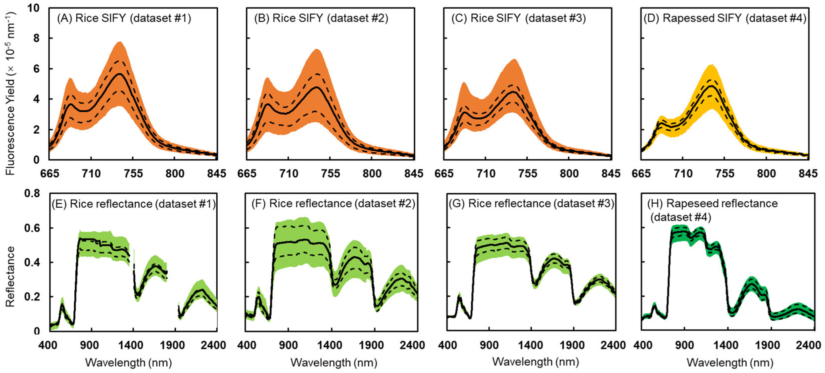
The SIFY and reflectance spectra of the four leaf datasets obtained from measurements are shown in Figure 2. The SIFY of the three rice datasets displayed a distinct peak at approximately 680 nm, showcasing considerable variability (Figure 2A–C), while the rapeseed dataset showed a less pronounced peak around 680 nm with relatively lower variability. (Figure 2D). Except for rice dataset #2, the variation observed in reflectance was not significant across the other datasets. Additionally, the rice reflectance was notably higher than that of the rapeseed datasets in the 1500–1800 nm and 2000–2300 nm spectral bands. In contrast, in the visible light band, the reflectance of the rapeseed dataset was lower than that of the rice dataset.
The attenuated peak around 680 nm in the SIFY spectra of rapeseed might be attributed to the thicker and more complex leaf structure of rapeseed leaves, resulting in a more pronounced reabsorption effect for SIF before 700 nm [34]. Moreover, both the rice and rapeseed datasets exhibited clear dual peaks, indicating that the samples used in all four datasets were grown under relatively normal nutrient and moisture levels [25,35], thereby avoiding changes in SIF signal characteristics due to environmental stress. The observed reflectance spectra showed variations across spectral bands associated with Cab (450–750 nm), mesophyll structure (800–1250 nm), water absorption (1300–2400 nm), and dry matter content (1600–2500 nm) [36]. Among these, the changes in bands related to mesophyll structure were the most noticeable. Except for rice dataset #2, the magnitude of variations in SIFY spectra was greater than that in reflectance spectra for the other three datasets.
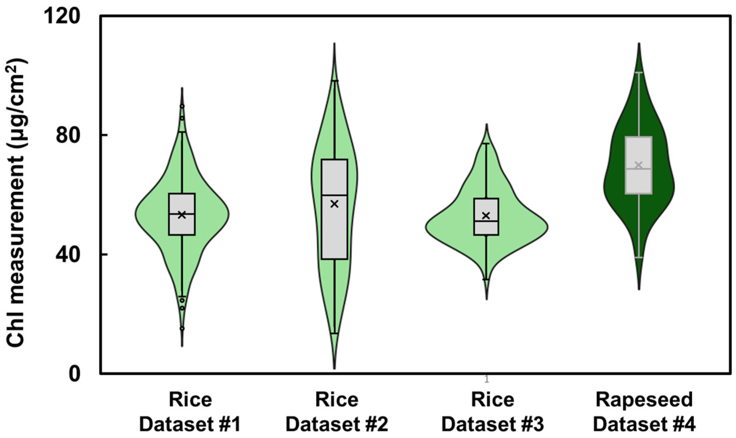
As shown in Figure 3, the means of the three rice datasets used in this study were relatively proximate, but their distributions differed. In terms of averages, they were in ascending order from rice dataset #3, #1, to #2, with a minimal difference between datasets #1 and #2. Concerning the maximum and minimum values, rice dataset #2 exhibited the broadest data distribution, ranging from 13.29 μg cm−2 to 96.83 μg cm−2. As shown in Table S2, rice dataset #2 exhibited a larger standard deviation, while dataset #3 had the smallest standard deviation. Detailed statistical data can be found in Table S2 in the Supplementary Materials. Conversely, rapeseed dataset #4 demonstrated the highest Cab, which elucidates why the reflectance of rapeseed dataset #4 had the lowest value in the visible light band.
Rice dataset #2, which had the widest distribution of Cab, also exhibited the largest variations in both SIFY and reflectance spectra. The narrower range of Cab in rice dataset #3 was attributed to the more precise fertilizer application in the potted cultivation medium compared to field conditions, ensuring that rice plants avoided nitrogen deficiency and progressed to the grain-filling stage.

3.2. Model Transferability between Different Rice Datasets

3.2.1. The Direct Transfer Results between Different Rice Datasets

The PLSR models demonstrated acceptable predictions of Cab using either SIFY or reflectance spectra. With the exception of predicting the Cab of rice dataset #1 using reflectance spectra from rice dataset #3 (Figure 4E), the R2 of the transfer models exceeded 0.5 in other cases. Additionally, except for this specific case (Figure 4E), transfer models based on reflectance spectra exhibited a lower RMSE compared to those based on SIFY. For transfer models based on SIFY, the average R2 and RMSE across different training sets were relatively close, with R2 ranging from 0.64 to 0.70 and RMSE ranging from 12.92 to 13.35 μg cm−2 (Table S3). In contrast, for transfer models based on reflectance spectra, the average R2 and RMSE across different dataset pairs were relatively close, with R2 ranging from 0.59 to 0.68 and RMSE ranging from 10.15 to 13.74 μg cm−2 (Table S4). When considering the average R2 and RMSE of the six transfer models (Figure 4A–F), there was little difference between those based on SIFY and reflectance spectra, with R2 of 0.67 and 0.64, respectively, and RMSE of 13.16 μg cm−2 and 13.30 μg cm−2, respectively.

3.2.2. Effects of Different Pretreatments and Model Updating Ratios on Model Transfer

The study investigated the transfer performance of models across diverse datasets and examined the impacts of spectral preprocessing techniques. The results of spectral preprocessed transfer models based on SIFY and reflectance are shown in Table 2 and Table 3, respectively. Across the transfer models based on SIFY, most preprocessing methods improved the model accuracy, with only a few cases where the performance was reduced. Compared to models without preprocessing, each transfer model showed an increase in R2 and a decrease in RMSE after applying the optimal preprocessing scheme. Specifically, the optimal results of the six transfer models showed an average increase in R2 of 0.05 and an average decrease in RMSE of 31.72%. Except for the mutual transfer between rice dataset #2 and rice dataset #3, where “MSC + SNV” was chosen as the optimal spectral preprocessing method, “MSC + FD” was the best preprocessing approach in other cases.
As shown in Table 3, compared to using SIFY as the data source, spectral preprocessing had limited effects on improving the transfer models based on reflectance, with only half of the cases showing improvements in both R2 and RMSE. Among the cases where improvements were observed, the “MSC + FD” scheme was still chosen by the majority of transfer models. Additionally, it was worth noting that spectral preprocessing significantly improved the performance of the worst-performing direct transfer model between rice datasets #3 and #1 (Figure 4E), with R2 increasing by 0.19 and RMSE decreasing by 60.74%.
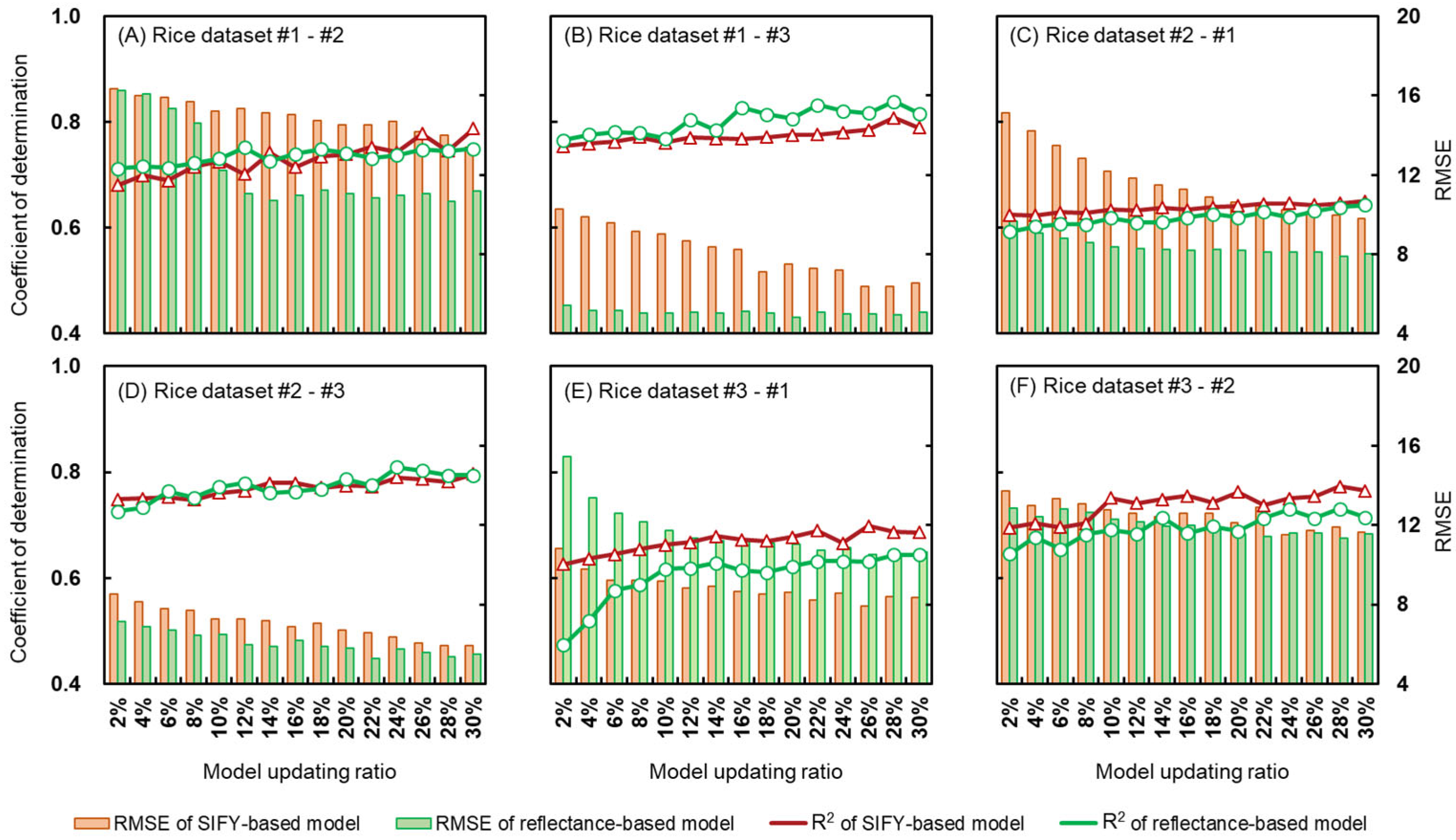
Moreover, model updating was conducted to enhance the Cab estimation achieved by both SIFY-based and reflectance-based models across different dataset pairs, as depicted in Figure 5. Through the transfer of samples from the target dataset to the source dataset, model updating resulted in improved Cab estimations. When the transferred data volume approached 30%, in almost all cases (except for rice datasets #2–#3, Figure 5D), both R2 and RMSE tended to stabilize. The accuracy gradually increased with the increase in the number of transferred samples, and when the transferred sample percentage exceeded 10%, R2 and RMSE showed a relatively stable trend in some cases (Figure 5A,C,E). Specifically, in Figure 5A,E, the R2 and RMSE of the reflectance-based models showed significant variation in the first 10% model updates; whereas in Figure 5C, the results of the SIFY-based model exhibited greater variation. However, for some cases where direct modeling already exhibited high accuracy, such as the reflectance transfer model from rice dataset #1 to rice dataset #2, the reduction in RMSE was not significant (Figure 5B). From the statistical results, when the transferred sample quantity reached 10% and 30% of the source dataset, the average R2 of the SIFY-based transfer models increased by 6.94% and 11.42%, respectively, while the RMSE decreased by 19.59% and 29.83%, respectively (Table S5). For the reflectance-based models, the average R2 increased by 11.96% and 16.30%, respectively, while the RMSE decreased by 25.89% and 27.01%, respectively (Table S6).
For the average R2 and RMSE, the improvement effect of the SIFY-based models at a data transfer rate of 10% accounted for over 60% of the improvement effect at a data transfer rate of 30%. For the reflectance-based models, these data reached over 70%. With only one-third of the data transfer volume, a significant improvement of over 60% was achieved in the models of both data sources, indicating that a data transfer rate of 10% can have a substantial impact.

3.3. Between-Species Data Transfer Results

Compared to intra-species transfer models, the results of between-species transfer showed notable differences. The SIFY-based models demonstrated relatively consistent predictive capabilities across the three rice datasets for rapeseed, with R2 ranging from 0.52 to 0.55 and RMSE ranging from 10.01 to 11.65 μg cm−2. However, the performance of the reflectance-based models in the between-species prediction was somewhat poorer; except for the predictive model based on the 2020 rice dataset #1 (Figure 6A, R2 = 0.63, RMSE = 10.14 μg cm−2), the other two cases were less satisfactory (R2 < 0.5, RMSE > 13 μg cm−2).
A total of 10% of the rapeseed samples were transferred into the source dataset, and the SIFY dataset was preprocessed using the “MSC + FD” approach, as shown in Figure 6D–F. Subsequently, there was a significant improvement in the predictive performance of between-species transfer models. For SIFY-based models, the R2 values increased by 0.12, 0.09, and 0.10, respectively, while the RMSE values decreased by 26.01%, 25.40%, and 19.38%. For reflectance-based models, the R2 values increased by 0.09, 0.31, and 0.49, respectively, with corresponding decreases in RMSE of 28.50%, 34.05%, and 43.53%.
The between-species transfer results amplified the conclusions obtained from direct modeling, revealing the constraints faced by reflectance-based models in scenarios where substantial discrepancies existed between the attributes of the training and testing sets. On the contrary, SIFY, an endogenous light closely correlated with chlorophyll, yielded acceptable results even in direct between-species predictions (Figure 6). Through model updating and spectral preprocessing, both between-species transfer models based on SIFY and reflectance can achieve a level of accuracy similar to that of intra-species transfer models across different rice datasets.

4. Discussion

The transfer model results in this study were slightly better than the Cab assessment models established by Wittenberghe [7] based on upward and downward SIFY. The weakest performance among SIFY-based models was observed between rice dataset #1 and dataset #2, possibly due to the limited overlap in cultivars between these two datasets (Table S1) and inconsistencies in nitrogen application levels, leading to variations in the chlorophyll-to-nitrogen ratio. This conclusion was supported by the chlorophyll-to-carotenoid ratio among different datasets (Figure S3). Most samples from rice dataset #1 and dataset #3 exhibited ratios between six and eight, while rice dataset #2 showed a higher proportion of samples with ratios exceeding eight, and even reaching ten or more in some cases. The chlorophyll-to-carotenoid ratio provides insights into leaf functionality because Cab varies dynamically throughout the plant growth cycle, while the carotenoid content remains relatively stable before advanced stage of senescence [37,38]. On the other hand, the reflectance-based model yielded results consistent with previous studies, such as Xiao [19] who established transfer models between different cotton cultivars with R2 ranging from 0.58 to 0.73. For the models based on reflectance spectra, those employing rice dataset #3 as the training set showed the worst average R2 and RMSE. This may be due to rice dataset #3 containing the fewest features; for instance, it lacked data pairs with Cab below 30 μg cm−2 or above 77 μg cm−2. Moreover, compared to rice dataset #2, rice dataset #1 also lacked data pairs with Cab higher than 88 μg cm−2, resulting in unsatisfactory prediction performance of the transfer models. After excluding the results of rice dataset #3 for predicting dataset #1, the transfer models based on reflectance (average R2 = 0.68 and RMSE = 10.64 μg cm−2) outperformed those based on SIFY (average R2 = 0.68 and RMSE = 13.23 μg cm−2). From the direct transfer results between the rice datasets, the transfer model based on SIFY showed relatively consistent predictive performance, albeit being influenced by the physiological status and biochemical composition ratios of the plants. In contrast, the transfer model based on reflectance required adequate learning of features in the training set to maintain good predictive capabilities, otherwise the prediction performance would be significantly influenced.
The most commonly selected preprocessing method, MSC, was originally applied in the near-infrared spectrum domain [39]. Its principle lies in eliminating the influence of scatter on the shape and intensity of spectra, thereby enhancing the accuracy of model establishment [40]. While scatter phenomena also occur in SIF within leaves [29], SIF does not exhibit the complex relationships coupled with various biochemical components, as seen in reflectance [41]. Therefore, MSC significantly augments the transfer learning performance of SIFY models. This study employed Savizkye–Golay smoothing followed by a first derivative calculation, a method that can remove background noise and enhance spectral resolution, making some less pronounced peaks and valleys in the original spectra more distinct [33]. Therefore, FD was applied to both SIFY-based and reflectance-based models.
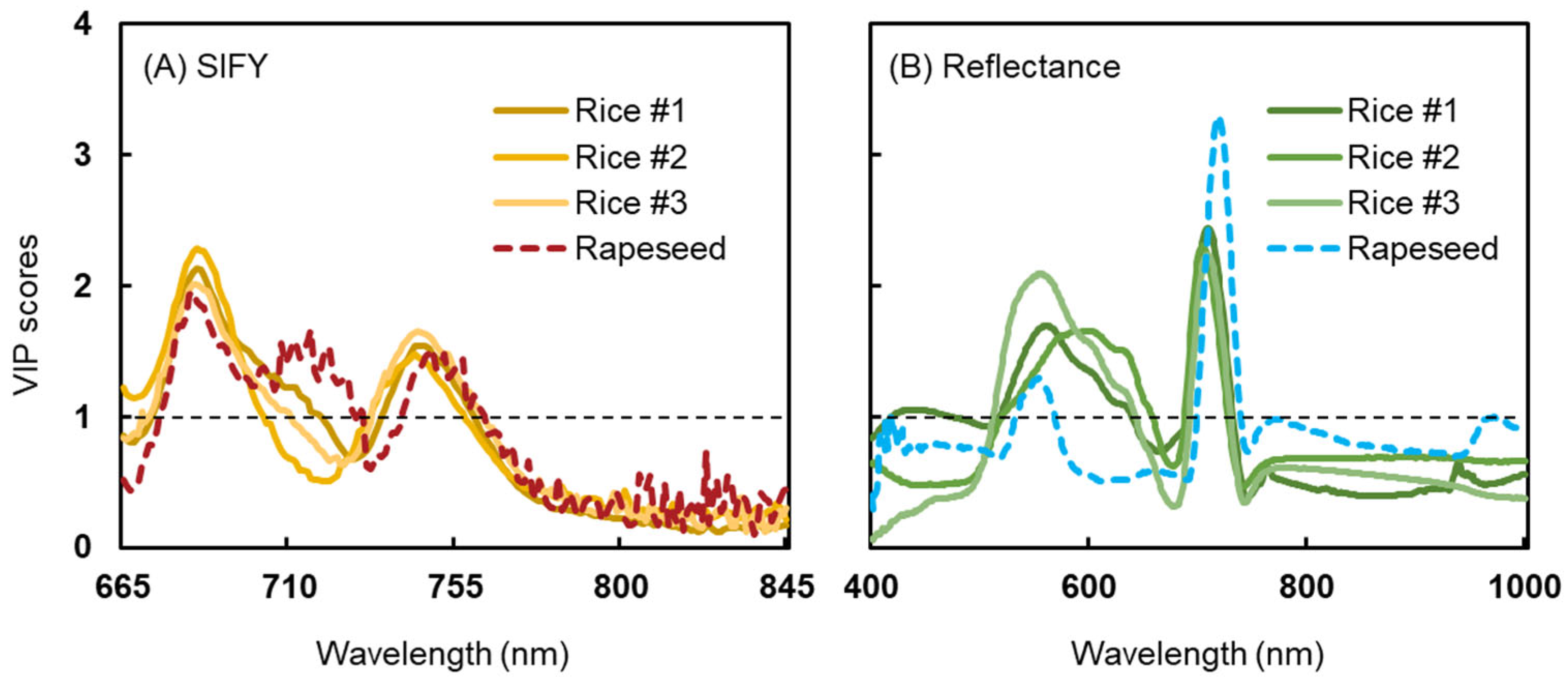
Figure 7 illustrates the importance of each SIFY and 400–1000 nm reflectance spectra band in the PLSR model. For SIFY spectra, except for the 710–730 nm band, the VIP scores for rice and rapeseed were very close in other bands, with peaks observed at 680 nm and 740 nm in both cases. Regarding reflectance, although there was some similarity in the trend lines of VIP scores between the rice and rapeseed datasets, such as exhibiting two peaks between 400–1000 nm and scores dropping below one after 740 nm, there were still many differences between them. The VIP scores of the three rice datasets exceeded one between 500–640 nm, while only the 540–570 nm VIP scores of the rapeseed dataset exceeded one. Additionally, the second peak position of all three rice datasets was approximately at 710 nm, while for rapeseed, it was close to 720 nm. The magnitudes of the peaks in rice datasets were relatively consistent, whereas the intensity of the second peak in rapeseed was nearly three times that of the first peak.
Compared to reflectance, the VIP score curves of the SIFY-based models for different species were more similar (Figure 7A), which may explain why SIFY-based models still performed well in direct between-species transfer. The 710–725 nm range, with different VIP scores in rice and rapeseed datasets, encompasses fluorescence emitted by both Photosystem I (PSI) and Photosystem II (PSII) [42]. Studies suggest that the ratio of PSII- to PSI-excited fluorescence may differ between different plant species [43]. As for reflectance, chlorophyll absorption predominates within the 660–680 nm range, resulting in low VIP scores. The red-edge reflectance in the 680–750 nm range is sensitive to chlorophyll while also avoiding interference from other pigments [44]. Consequently, it has been widely recognized as an important spectral band for assessing chlorophyll levels, for instance, in the development of vegetation indices like the CIred-edge [45]. The red-edge bands in the reflectance-based models exhibited the highest VIP scores, which were especially notable in the rapeseed dataset when compared to other bands. However, a significant disparity in VIP scores between the rice and rapeseed datasets was observed within the 550–650 nm range, corresponding closely to wavelengths strongly associated with leaf Cab in the original spectra. This limitation hinders the between-species applicability of the reflectance model. Prior to 450 nm, both rice dataset #1 and rapeseed datasets showed relatively similar VIP scores, and studies has demonstrated a strong correlation between the first derivative spectra and chlorophyll within the 450–500 nm range [36], which may explain why rice dataset #1 performed the best in the between-species prediction.
Therefore, this study proposes that when predicting species using existing extensive datasets without introducing new datasets, reflectance should be given consideration. Because when the features of the training set are sufficient, it often performs better. The best original transfer model used in this study was based on reflectance (Figure 4B). However, in scenarios where there is no pre-existing dataset for the target species, employing SIF would be preferable because of its robustness. All original transfer models constructed based on SIF in this study had an R2 exceeding 0.5. The limitation of this study may lie in the fact that although the datasets used included dozens of varieties and materials and various planting methods, the sample size was still limited. Canola and rice are both C3 crops, and considering that the photosynthetic processes of C3 and C4 plants are not completely consistent, further validation may be needed in more species in the future. Compared to the well-established and extensive databases for reflectance, such as EcoSIS [46], there are relatively few publicly available datasets that simultaneously have SIF measurements and corresponding biochemical components of leaf samples. This study advocates for the establishment of databases for SIF and SIFY, along with conducting data mining and innovative research based on these datasets. Such endeavors would facilitate explorations of the correlations and regularities between SIF and various biochemical components and photosynthetic parameters, thereby contributing to the advancement of knowledge in this research domain.

5. Conclusions

The study findings demonstrated that PLSR models based on reflectance and SIFY spectra both possess transferability for Cab estimations. After spectral preprocessing and data transfer, models utilizing both reflectance and SIFY spectra demonstrated notable between-species predictive abilities. In particular, in scenarios where the training dataset featured fewer sample attributes, SIFY-based models showcased enhanced robustness, yielding R2 values surpassing 0.5 for both inter-species and between-species direct transfer models, whereas reflectance-based models performed better with more sample attributes. Spectral preprocessing techniques enhanced the transfer performance of the models, particularly for SIFY-based models. Moreover, updating the data significantly improved the transferability of both reflectance-based and SIFY-based models, with an approximately 10% augmentation in the transfer dataset typically resulting in a significant improvement in model accuracy. The proposed methods minimize the necessity for supplementary data, extending the initial model’s predictive capacity for Cab to diverse species, thereby reducing production costs by leveraging existing extensive crop datasets.
However, since the datasets employed in this study exclusively consisted of C3 crops, future research endeavors may delve into examining the transferability of alternative physiological and biochemical parameters. This could be achieved by incorporating datasets from a wider variety of species, thereby expanding and refining the findings delineated in this study.

Supplementary Materials

The following supporting information can be downloaded at https://www.mdpi.com/article/10.3390/rs16111869/s1: Table S1. The detailed cultivars and materials included in each dataset. Table S2. Summary of statistical data for the chlorophyll content in each dataset. Mean, standard deviation, minimum, and maximum values of chlorophyll content were given (unit: μg cm−2). Table S3. The R2 and RMSE of transfer models based on SIFY spectra averaged across different datasets or training sets. Table S4. The R2 and RMSE of transfer models based on reflectance spectra averaged across different datasets or training sets. Table S5. The R2 and RMSE of the transfer models based on SIFY with different model update ratios, as well as the changes in predictive performance compared to no processing. Table S6. The R2 and RMSE of the transfer models based on reflectance with different model update ratios, as well as the changes in predictive performance compared to no processing. Figure S1. Photosynthetic energy partitioning and leaf structure. The green arrow represents reflected radiation and the red arrow represents sun-induced chlorophyll fluorescence, both of which are easy-to-capture remote sensing signals. Figure S2. Schematic of the FluoWat leaf clip. Reflectance (R) and transmittance (T) are measured by placing a fiber optic either in the upward (↑) or downward (↓) position (subplot A). After placing the shortpass filter to restrict incoming PAR to visible wavelengths up to 650 nm (subplot B), upward and downward sun-induced fluorescence (↑SIF, ↓SIF) are measured. The total light arriving at the sample is obtained by measuring with the white reference, then PAR absorbed by the sample is calculated through the R and T obtained from the subplot A, and finally the SIF yield is obtained (subplot C). Figure S3. The chlorophyll-to-carotenoid ratios among different datasets. The datasets are sorted by the magnitude of the ratio.

Author Contributions

Conceptualization, H.C.; methodology, Y.-a.Z.; software, Y.-a.Z.; investigation, H.C. and W.Z.; resources, W.Z.; data curation, Y.-a.Z.; writing—original draft preparation, Y.-a.Z.; writing—review and editing, Z.H. and H.C.; visualization, Y.-a.Z.; funding acquisition, H.C. All authors have read and agreed to the published version of the manuscript.

Funding

This research was supported by the Fundamental Research Funds for the Central Universities (226-2022-00217), the Key R&D Program of Zhejiang Province (2021C02057), and Zhejiang University Global Partnership Fund (188170+194452208/005).

Data Availability Statement

All data used to support the findings of this study are included within the article.

Conflicts of Interest

The authors declare no conflicts of interest.

References

  1. Gitelson, A.A.; Peng, Y.; Arkebauer, T.J.; Schepers, J. Relationships between gross primary production, green LAI, and canopy chlorophyll content in maize: Implications for remote sensing of primary production. Remote Sens. Environ. 2014, 144, 65–72. [Google Scholar] [CrossRef]
  2. Richardson, A.D.; Duigan, S.P.; Berlyn, G.P. An evaluation of noninvasive methods to estimate foliar chlorophyll content. New Phytol. 2002, 153, 185–194. [Google Scholar] [CrossRef]
  3. Andrianto, H.; Faizal, A. Measurement of chlorophyll content to determine nutrition deficiency in plants: A systematic literature review. In Proceedings of the 2017 International Conference on Information Technology Systems and Innovation (ICITSI), Bandung, Indonesia, 23–24 October 2017; pp. 392–397. [Google Scholar]
  4. Kior, A.; Sukhov, V.; Sukhova, E. Application of Reflectance Indices for Remote Sensing of Plants and Revealing Actions of Stressors. Photonics 2021, 8, 582. [Google Scholar] [CrossRef]
  5. Verrelst, J.; Muñoz, J.; Alonso, L.; Delegido, J.; Rivera, J.P.; Camps-Valls, G.; Moreno, J. Machine learning regression algorithms for biophysical parameter retrieval: Opportunities for Sentinel-2 and -3. Remote Sens. Environ. 2012, 118, 127–139. [Google Scholar] [CrossRef]
  6. Chang, S.X.; Robison, D.J. Nondestructive and rapid estimation of hardwood foliar nitrogen status using the SPAD-502 chlorophyll meter. For. Ecol. Manag. 2003, 181, 331–338. [Google Scholar] [CrossRef]
  7. Van Wittenberghe, S.; Verrelst, J.; Rivera, J.P.; Alonso, L.; Moreno, J.; Samson, R. Gaussian processes retrieval of leaf parameters from a multi-species reflectance, absorbance and fluorescence dataset. J. Photochem. Photobiol. B 2014, 134, 37–48. [Google Scholar] [CrossRef]
  8. Sims, D.A.; Gamon, J.A. Relationships between leaf pigment content and spectral reflectance across a wide range of species, leaf structures and developmental stages. Remote Sens. Environ. 2002, 81, 337–354. [Google Scholar] [CrossRef]
  9. Slaton, M.R.; Raymond Hunt, E.; Smith, W.K. Estimating near-infrared leaf reflectance from leaf structural characteristics. Am. J. Bot. 2001, 88, 278–284. [Google Scholar] [CrossRef] [PubMed]
  10. Serrano, L. Effects of leaf structure on reflectance estimates of chlorophyll content. Int. J. Remote Sens. 2010, 29, 5265–5274. [Google Scholar] [CrossRef]
  11. Esteban, R.; Fernández-Marín, B.; Hernandez, A.; Jiménez, E.T.; León, A.; García-Mauriño, S.; Silva, C.D.; Dolmus, J.R.; Dolmus, C.M.; Molina, M.J.; et al. Salt crystal deposition as a reversible mechanism to enhance photoprotection in black mangrove. Trees 2012, 27, 229–237. [Google Scholar] [CrossRef]
  12. Feng, L.; Wu, B.; He, Y.; Zhang, C. Hyperspectral Imaging Combined with Deep Transfer Learning for Rice Disease Detection. Front. Plant Sci. 2021, 12, 693521. [Google Scholar] [CrossRef] [PubMed]
  13. Berger, K.; Verrelst, J.; Féret, J.-B.; Wang, Z.; Wocher, M.; Strathmann, M.; Danner, M.; Mauser, W.; Hank, T. Crop nitrogen monitoring: Recent progress and principal developments in the context of imaging spectroscopy missions. Remote Sens. Environ. 2020, 242, 111758. [Google Scholar] [CrossRef] [PubMed]
  14. Verrelst, J.; Malenovsky, Z.; Van der Tol, C.; Camps-Valls, G.; Gastellu-Etchegorry, J.P.; Lewis, P.; North, P.; Moreno, J. Quantifying Vegetation Biophysical Variables from Imaging Spectroscopy Data: A Review on Retrieval Methods. Surv. Geophys. 2019, 40, 589–629. [Google Scholar] [CrossRef] [PubMed]
  15. Yin, X.; Struik, P.C.; Goudriaan, J. On the needs for combining physiological principles and mathematics to improve crop models. Field Crops Res. 2021, 271, 108254. [Google Scholar] [CrossRef]
  16. Brodzicki, A.; Piekarski, M.; Kucharski, D.; Jaworek-Korjakowska, J.; Gorgon, M. Transfer Learning Methods as a New Approach in Computer Vision Tasks with Small Datasets. Found. Comput. Decis. Sci. 2020, 45, 179–193. [Google Scholar] [CrossRef]
  17. Wan, G.; Yu, A.; Yu, X.; Liu, B. Deep convolutional recurrent neural network with transfer learning for hyperspectral image classification. J. Appl. Remote Sens. 2018, 12, 026028. [Google Scholar] [CrossRef]
  18. Qiao, L.; Mu, Y.; Lu, B.; Tang, X. Calibration Maintenance Application of Near-infrared Spectrometric Model in Food Analysis. Food Rev. Int. 2021, 39, 1628–1644. [Google Scholar] [CrossRef]
  19. Xiao, Q.; Tang, W.; Zhang, C.; Zhou, L.; Feng, L.; Shen, J.; Yan, T.; Gao, P.; He, Y.; Wu, N. Spectral Preprocessing Combined with Deep Transfer Learning to Evaluate Chlorophyll Content in Cotton Leaves. Plant Phenomics 2022, 2022, 9813841. [Google Scholar] [CrossRef] [PubMed]
  20. Wan, L.; Zhou, W.; He, Y.; Wanger, T.C.; Cen, H. Combining transfer learning and hyperspectral reflectance analysis to assess leaf nitrogen concentration across different plant species datasets. Remote Sens. Environ. 2022, 269, 112826. [Google Scholar] [CrossRef]
  21. Meacham-Hensold, K.; Montes, C.M.; Wu, J.; Guan, K.; Fu, P.; Ainsworth, E.A.; Pederson, T.; Moore, C.E.; Brown, K.L.; Raines, C.; et al. High-throughput field phenotyping using hyperspectral reflectance and partial least squares regression (PLSR) reveals genetic modifications to photosynthetic capacity. Remote Sens. Environ. 2019, 231, 111176. [Google Scholar] [CrossRef]
  22. Stirbet, A.; Lazar, D.; Guo, Y.; Govindjee, G. Photosynthesis: Basics, history and modelling. Ann. Bot. 2020, 126, 511–537. [Google Scholar] [CrossRef] [PubMed]
  23. Guan, K.; Berry, J.A.; Zhang, Y.; Joiner, J.; Guanter, L.; Badgley, G.; Lobell, D.B. Improving the monitoring of crop productivity using spaceborne solar-induced fluorescence. Glob. Chang. Biol. 2016, 22, 716–726. [Google Scholar] [CrossRef] [PubMed]
  24. Tubuxin, B.; Rahimzadeh-Bajgiran, P.; Ginnan, Y.; Hosoi, F.; Omasa, K. Estimating chlorophyll content and photochemical yield of photosystem II (PhiPSII) using solar-induced chlorophyll fluorescence measurements at different growing stages of attached leaves. J. Exp. Bot. 2015, 66, 5595–5603. [Google Scholar] [CrossRef] [PubMed]
  25. Jia, M.; Zhu, J.; Ma, C.; Alonso, L.; Li, D.; Cheng, T.; Tian, Y.; Zhu, Y.; Yao, X.; Cao, W. Difference and Potential of the Upward and Downward Sun-Induced Chlorophyll Fluorescence on Detecting Leaf Nitrogen Concentration in Wheat. Remote Sens. 2018, 10, 1315. [Google Scholar] [CrossRef]
  26. Fu, P.; Meacham-Hensold, K.; Siebers, M.H.; Bernacchi, C.J. The inverse relationship between solar-induced fluorescence yield and photosynthetic capacity: Benefits for field phenotyping. J. Exp. Bot. 2021, 72, 1295–1306. [Google Scholar] [CrossRef] [PubMed]
  27. Magney, T.S.; Frankenberg, C.; Köhler, P.; North, G.; Davis, T.S.; Dold, C.; Dutta, D.; Fisher, J.B.; Grossmann, K.; Harrington, A.; et al. Disentangling Changes in the Spectral Shape of Chlorophyll Fluorescence: Implications for Remote Sensing of Photosynthesis. J. Geophys. Res. Biogeosci. 2019, 124, 1491–1507. [Google Scholar] [CrossRef]
  28. Van Wittenberghe, S.; Alonso, L.; Verrelst, J.; Hermans, I.; Delegido, J.; Veroustraete, F.; Valcke, R.; Moreno, J.; Samson, R. Upward and downward solar-induced chlorophyll fluorescence yield indices of four tree species as indicators of traffic pollution in Valencia. Environ. Pollut. 2013, 173, 29–37. [Google Scholar] [CrossRef]
  29. Van Wittenberghe, S.; Alonso, L.; Verrelst, J.; Moreno, J.; Samson, R. Bidirectional sun-induced chlorophyll fluorescence emission is influenced by leaf structure and light scattering properties—A bottom-up approach. Remote Sens. Environ. 2015, 158, 169–179. [Google Scholar] [CrossRef]
  30. Chen, S.; Zhai, L.; Zhou, Y.; Xie, J.; Shao, Y.; Wang, W.; Li, H.; He, Y.; Cen, H. Early diagnosis and mechanistic understanding of citrus Huanglongbing via sun-induced chlorophyll fluorescence. Comput. Electron. Agric. 2023, 215, 108357. [Google Scholar] [CrossRef]
  31. Wold, S.; Sjostrom, M.; Eriksson, L. PLS-regression: A basic tool of chemometrics. Chemometrics and Intelligent Laboratory Systems 2001, 58, 109–130. [Google Scholar] [CrossRef]
  32. Farrés, M.; Platikanov, S.; Tsakovski, S.; Tauler, R. Comparison of the variable importance in projection (VIP) and of the selectivity ratio (SR) methods for variable selection and interpretation. J. Chemom. 2015, 29, 528–536. [Google Scholar] [CrossRef]
  33. Cen, H.; He, Y. Theory and application of near infrared reflectance spectroscopy in determination of food quality. Trends Food Sci. Technol. 2007, 18, 72–83. [Google Scholar] [CrossRef]
  34. Buschmann, C. Variability and application of the chlorophyll fluorescence emission ratio red/far-red of leaves. Photosynth. Res. 2007, 92, 261–271. [Google Scholar] [CrossRef] [PubMed]
  35. Xu, S.; Liu, Z.; Han, S.; Chen, Z.; He, X.; Zhao, H.; Ren, S. Exploring the Sensitivity of Solar-Induced Chlorophyll Fluorescence at Different Wavelengths in Response to Drought. Remote Sens. 2023, 15, 1077. [Google Scholar] [CrossRef]
  36. Zhu, J.; He, W.; Yao, J.; Yu, Q.; Xu, C.; Huang, H.; Mhae, B.; Jandug, C. Spectral Reflectance Characteristics and Chlorophyll Content Estimation Model of Quercus aquifolioides Leaves at Different Altitudes in Sejila Mountain. Appl. Sci. 2020, 10, 3636. [Google Scholar] [CrossRef]
  37. Féret, J.B.; Gitelson, A.A.; Noble, S.D.; Jacquemoud, S. PROSPECT-D: Towards modeling leaf optical properties through a complete lifecycle. Remote Sens. Environ. 2017, 193, 204–215. [Google Scholar] [CrossRef]
  38. Spafford, L.; le Maire, G.; MacDougall, A.; de Boissieu, F.; Féret, J.-B. Spectral subdomains and prior estimation of leaf structure improves PROSPECT inversion on reflectance or transmittance alone. Remote Sens. Environ. 2021, 252, 112176. [Google Scholar] [CrossRef]
  39. Geladi, P.; MacDougall, D.; Martens, H. Linearization and Scatter-Correction for Near-Infrared Reflectance Spectra of Meat. Appl. Spectrosc. 1985, 39, 491–500. [Google Scholar] [CrossRef]
  40. Isaksson, T.; Næs, T. The effect of multiplicative scatter correction (MSC) and linearity improvement in NIR spectroscopy. Appl. Spectrosc. 1988, 42, 1273–1284. [Google Scholar] [CrossRef]
  41. Ollinger, S.V. Sources of variability in canopy reflectance and the convergent properties of plants. New Phytol. 2011, 189, 375–394. [Google Scholar] [CrossRef]
  42. Porcar-Castell, A.; Malenovsky, Z.; Magney, T.; Van Wittenberghe, S.; Fernandez-Marin, B.; Maignan, F.; Zhang, Y.; Maseyk, K.; Atherton, J.; Albert, L.P.; et al. Chlorophyll a fluorescence illuminates a path connecting plant molecular biology to Earth-system science. Nat. Plants 2021, 7, 998–1009. [Google Scholar] [CrossRef] [PubMed]
  43. Peterson, R.B.; Oja, V.; Eichelmann, H.; Bichele, I.; Dall’Osto, L.; Laisk, A. Fluorescence F 0 of photosystems II and I in developing C3 and C 4 leaves, and implications on regulation of excitation balance. Photosynth. Res. 2014, 122, 41–56. [Google Scholar] [CrossRef] [PubMed]
  44. Horler, D.; Dockray, M.; Barber, J. The red edge of plant leaf reflectance. Int. J. Remote Sens. 1983, 4, 273–288. [Google Scholar] [CrossRef]
  45. Gitelson, A.A.; Gritz, Y.; Merzlyak, M.N. Relationships between leaf chlorophyll content and spectral reflectance and algorithms for non-destructive chlorophyll assessment in higher plant leaves. J. Plant Physiol. 2003, 160, 271–282. [Google Scholar] [CrossRef] [PubMed]
  46. Wagner, E.P.; Merz, J.; Townsend, P.A. EcoSIS: A spectral library and the tools to use it. In Proceedings of the AGU Fall Meeting, San Francisco, CA, USA, 9–13 December 2019; p. B11F-2396. [Google Scholar]
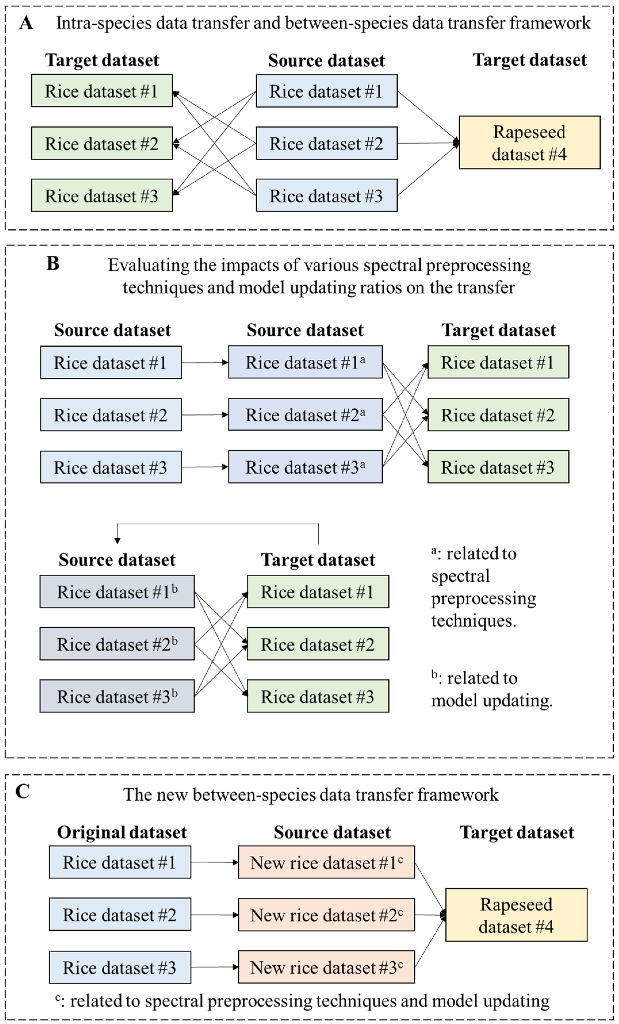
Figure 1. Architecture of the transfer learning method for estimating the leaf chlorophyll content across different datasets. (A) The transfer effects between different rice datasets and between-species transfer effects. (B) Determination of the optimal spectral preprocessing scheme using different spectral preprocessing techniques and their combinations, and exploration of the best transfer ratio by updating the model by transferring samples from the target dataset to the source dataset. (C) Between-species transfer effects after using the optimal spectral preprocessing scheme and transfer ratio for the source dataset. Each step in the framework diagram utilizes both reflectance and SIFY spectra.
Remotesensing 16 01869 g001
Figure 2. Overview of upward SIFY (AD) and reflectance (EH) spectra of the four datasets. The average spectra (continuous black line), the first and third quartiles (dashed black lines), and the range of all measured spectra (shaded area) are shown. In particular, the rapeseed dataset is represented using colors from the same color family but with different shades (D,H). Since the reflectance of dataset #1 is calculated by irradiance, the 1350–1400 nm and 1800–1940 nm bands affected by water absorption were removed.
Remotesensing 16 01869 g002
Figure 3. Violin and box plots of chlorophyll measurement values for four datasets. The boxes show the interquartile range with the median as a solid horizontal line. Whiskers show data outside the interquartile range but within 1.5× the interquartile range. Dots show outliers. Specifically, the rapeseed dataset is represented in a deeper shade of green.
Remotesensing 16 01869 g003
Figure 4. Transfer learning for assessing the chlorophyll content across different rice datasets. For example, “rice dataset #1–#2” indicates the use of the PLSR models established from rice dataset #1 to estimate the chlorophyll content of rice dataset #2. The black dashed line presents the 1:1 line, and the color dashed lines represent the linear regression fit to the data. The green color represents reflectance-based models, while the orange color represents SIFY-based models. RMSE (unit, μg cm−2) and R2 are inset for each graph.
Remotesensing 16 01869 g004
Figure 5. Transfer learning with model updating for assessing chlorophyll contents across different datasets. For example, “rice dataset #1–#2” indicates the use of the PLSR models established from rice dataset #1 to estimate the chlorophyll content of rice dataset #2. All figures use the same legend, which is located below the horizontal axis. The blue color represents reflectance-based models, while the orange color represents SIFY-based models. The bar chart represents the results for RMSE, while the line chart represents the results for R2.
Remotesensing 16 01869 g005
Figure 6. Results for the predicted chlorophyll content in the rapeseed dataset using models constructed based on different original rice datasets (AC) and rice datasets after spectral pretreatment and model updating (DF). The green color represents reflectance-based models, while the orange color represents SIFY-based models. RMSE and R2 are inset for each graph. Datasets marked with * indicate that spectral preprocessing techniques and model updating have been applied to them.
Remotesensing 16 01869 g006
Figure 7. Variable importance in projection (VIP) scores for the partial least-squares (PLS) regression models of the four datasets. Variables with a VIP score greater than 1 are considered important for the projection of the PLSR models.
Remotesensing 16 01869 g007
Table 1. Description of the three rice leaf datasets and the rapeseed leaf dataset.
DatasetPlantsLocationsNumber of SamplesPlanting MethodsYears
#112 rice cultivars and 15 rice materialsCNRRI and WHADP356Field and potted plants2020
#22 rice cultivarsCNRRI119Field2021
#32 rice cultivarsCNRRI149Potted plants2022
#46 rapeseed cultivarsARSZJU49Field2021–2022
Table 2. Results of transfer models built on different preprocessed SIFY spectra. For example, “rice dataset #1–#2” indicates the use of the PLSR models established from rice dataset #1 to estimate the chlorophyll content of rice dataset #2. The numbers in bold highlight models with relatively good results (unit for RMSE: μg cm−2).
PretreatmentR2 and RMSE
Rice Dataset
#1–#2
Rice Dataset
#1–#3
Rice Dataset
#2–#1
Rice Dataset
#2–#3
Rice Dataset
#3–#1
Rice Dataset
#3–#2
None0.6617.460.749.240.6116.490.739.340.6012.810.6813.62
MSC 10.7217.450.578.620.6216.970.757.260.6310.990.7811.37
SNV 20.7216.910.578.070.4818.270.757.980.6512.120.6512.12
FD 30.5717.250.738.130.6115.100.686.450.5511.500.5913.89
MSC + SNV0.7216.630.8010.430.6218.200.756.360.6312.080.7811.16
MSC + FD0.7412.270.796.000.629.530.7512.820.658.540.7511.43
SNV + FD0.7117.20.808.980.6218.70.779.260.6311.690.7511.28
1 MSC stands for multiplicative scatter correction. 2 SNV stands for standard normal variate transformation. 3 FD stands for first derivative.
Table 3. Results of transfer models built on different preprocessed reflectance spectra. For example, “rice dataset #1–#2” indicates the use of the PLSR models established from rice dataset #1 to estimate the chlorophyll content of rice dataset #2. The numbers in bold highlight models with relatively good results.
PretreatmentR2 and RMSE
Rice Dataset
#1–#2
Rice Dataset
#1–#3
Rice Dataset
#2–#1
Rice Dataset
#2–#3
Rice Dataset
#3–#1
Rice Dataset
#3–#2
None0.6916.320.735.410.5911.160.737.230.4426.620.6313.07
MSC 10.7114.700.726.070.6012.630.737.930.6313.700.7212.12
SNV 20.7114.850.725.960.6012.260.737.920.5813.890.7212.66
FD 30.6114.480.718.280.5011.030.697.470.5914.610.6512.96
MSC + SNV0.7114.940.725.960.6012.270.737.430.6312.350.7212.25
MSC + FD0.7113.340.775.970.5913.060.696.980.6310.450.7511.78
SNV + FD0.7213.170.616.510.6113.540.707.000.6413.810.7511.85
1 MSC stands for multiplicative scatter correction. 2 SNV stands for standard normal variate transformation. 3 FD stands for first derivative.
Disclaimer/Publisher’s Note: The statements, opinions and data contained in all publications are solely those of the individual author(s) and contributor(s) and not of MDPI and/or the editor(s). MDPI and/or the editor(s) disclaim responsibility for any injury to people or property resulting from any ideas, methods, instructions or products referred to in the content.