Chlorophyll-a Estimation in 149 Tropical Semi-Arid Reservoirs Using Remote Sensing Data and Six Machine Learning Methods

Abstract

It is crucial to monitor algal blooms in freshwater reservoirs through an examination of chlorophyll-a (Chla) concentrations, as they indicate the trophic condition of these waterbodies. Traditional monitoring methods, however, are expensive and time-consuming. Addressing this hindrance, we conducted a comprehensive investigation using several machine learning models for Chla modeling. To this end, we used in situ collected water sample data and remote sensing data from the Sentinel-2 satellite, including spectral bands and indices, for large-scale coverage. This approach allowed us to conduct a comprehensive analysis and characterization of the Chla concentrations across 149 freshwater reservoirs in Ceará, a semi-arid region of Brazil. The implemented machine learning models included k-nearest neighbors, random forest, extreme gradient boosting, the least absolute shrinkage, and the group method of data handling (GMDH); in particular, the GMDH approach has not been previously explored in this context. The forward stepwise approach was used to determine the best subset of input parameters. Using a 70/30 split for the training and testing datasets, the best-performing model was the GMDH model, achieving an R² of 0.91, an MAPE of 102.34%, and an RMSE of 20.4 μg/L, which were values consistent with the ones found in the literature. Nevertheless, the predicted Chla concentration values were most sensitive to the red, green, and near-infrared bands.

1. Introduction

Chlorophyll-a (Chla), a photosynthetic pigment in major algae groups, is widely used as a critical indicator of phytoplankton presence [1,2]. As the abundance of algae can reflect the state of eutrophication, Chla is one of the most important parameters for evaluating the trophic condition of water bodies [3,4]. While Chla concentration has long served as a critical parameter in monitoring harmful algal blooms, accurately predicting Chla concentration in reservoirs has proven to be a persistent challenge [5,6]. This difficulty is mainly due to the non-linear and non-stationary characteristics of Chla concentration, which are influenced by anthropogenic and hydrometeorological factors [7].

Regularly monitoring Chla concentrations is crucial for effective water quality management, as it helps prevent further deterioration [8]. However, traditional sampling methods are expensive, time-consuming, and impractical for many reservoirs [9,10]. Satellite remote sensing offers a cost-effective approach for monitoring Chla concentrations and their spatiotemporal variations, providing large-scale data on complex environmental systems [11]. In this context, because of its improved spatial resolution, the Sentinel-2 constellation has demonstrated its value in monitoring inland and coastal waters, setting it apart from other freely available remote sensing systems, such as Landsat 8 [12,13].

Estimations of Chla concentrations from remote sensing data can be achieved using machine learning (ML). The ML approach retrieves complex non-linear relationships within satellite data by capturing the underlying structure connecting the satellite data and the desired target variable [14,15]. Combining ML architectures with remote sensing data has been used to successfully monitor Chla in inland and ocean waters. For ocean waters, including coastal waters, specific Chla ML forecasting models using Sentinel-3 satellite data, namely the OLCI Neural Network Swarm (ONNS) and Ocean Colour 4 for MERIS (OC4ME), showed good performance for such a task [16,17].

In a previous study, a random forest (RF)-based model was developed for inland waters [18]. The authors used Sentinel-2 imagery to estimate Chla concentrations in Lake Chagan in China. Their proposed model provided good performance in determining Chla concentrations while complying with the biological mechanism in lakes, offering results that were robust to seasonal changes. Cao et al. [3] used Landsat-8 remote sensing data together with an extreme gradient boosting tree model (XGBoost) to determine Chla concentrations in lakes located in China. Their approach was implemented to analyze spatiotemporal data from 2013 to 2018 and demonstrated satisfactory performance in identifying the Chla behavior in the study location. Hu et al. [19] developed methodologies to mitigate spectral noise in remote sensing data from several satellites to improve the performance of ML models in estimating Chla concentrations in global oceans. Their results proved that the support vector regression (SVR) model was the best-performing ML approach, surpassing the traditional band-ratio models and providing reduced image noise.

The group method of data handling (GMDH) has also been applied to hydrological scenarios, including Chla estimation [20], water quality prediction [21], and image classification for plant diseases [22]. However, there is a gap in the knowledge regarding the usage of this approach in modeling Chla concentrations using satellite data, which the present study aims to fulfill. A proper investigation of the capacity of the GMDH to model Chla concentrations can contribute significantly to the development of real-time monitoring tools, as this approach does not require parameter tuning and has a fast processing time.

Another major contribution of the present study is to provide in-depth insight into the performance of several ML paradigms when applied to a vast area containing heterogeneous reservoirs. This proposed methodology is paramount in promoting the development of a more general ML structure able to provide accurate and precise results for a vast area. Given that reservoirs in semi-arid regions are often poorly monitored, the potential of algal blooms and further degradation of these aquatic systems have increased the need to study them. Therefore, this study aims to estimate Chla concentrations by combining remote sensing data and machine learning techniques. The following specific objectives were pursued in this research:

• A comprehensive investigation of several input parameters for Chla modeling, including all of the 13 bands registered by the MSI on board the Sentinel-2 constellation and 16 different spectral indices.
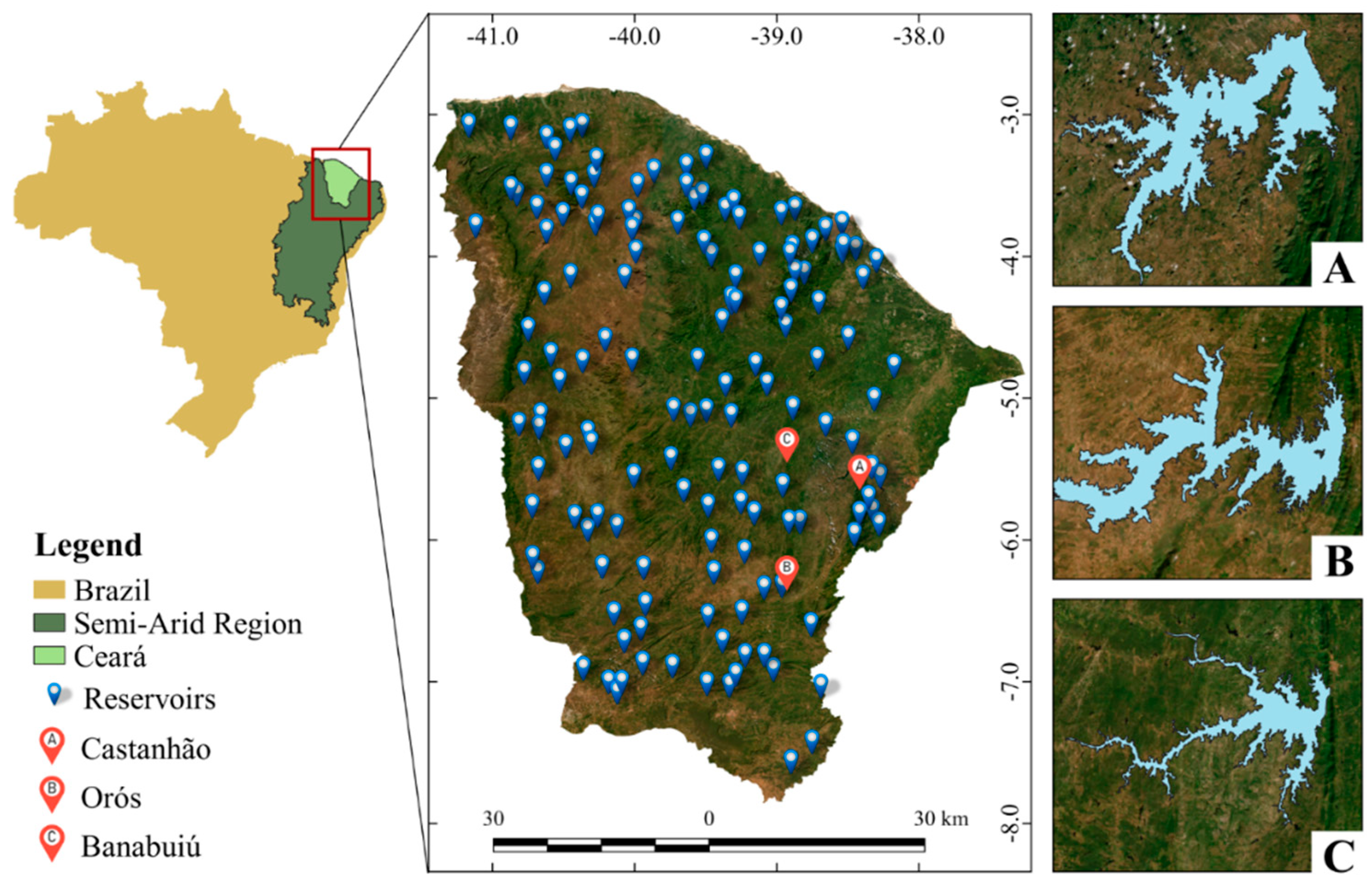
• A comprehensive analysis and characterization of all of the 149 tropical reservoirs that extensively spread across the state of Ceará, a Brazilian semi-arid region.
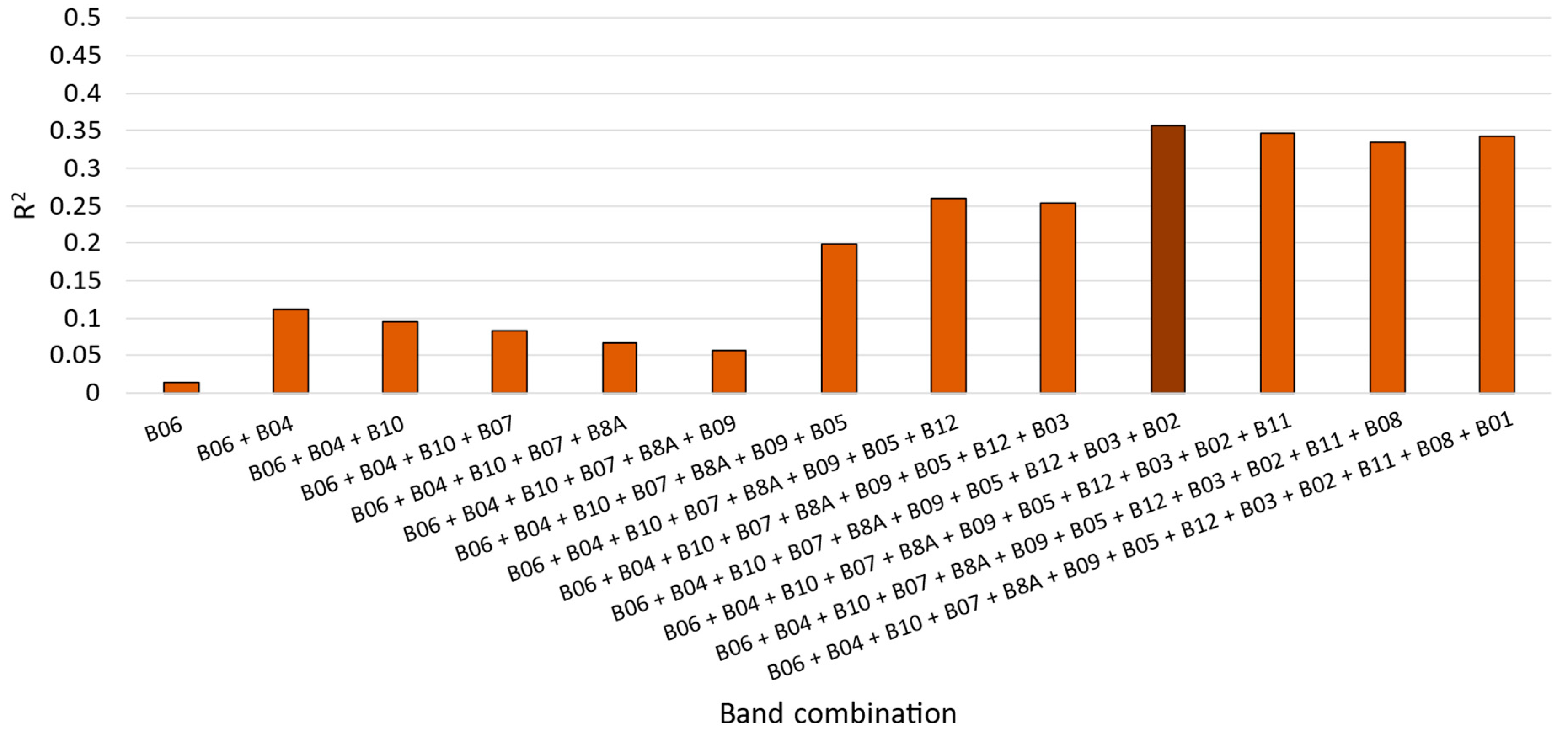
• The usage of the forward stepwise approach for parameter selection.
• The investigation of different machine learning paradigms for modeling Chla values in heterogeneous reservoirs distributed over a vast region.
• The usage of the GMDH ML model for Chla modeling using remote sensing data and spectral indices to fill the current knowledge gap.

2. Materials and Methods

2.1. Study Site Location

According to the Köppen classification [23], a semi-arid climate is classified as ‘BSh’ and is characterized by a mean precipitation of 750 mm per year, a potential evaporation rate of 2000 mm per year, a mean annual temperature of 31 °C, and negative water balances for most of the year [24,25]. In semi-arid regions, such as northeastern Brazil, which has approximately 28 million inhabitants in an area that occupies 12% of the national territory [26], the establishment of an extensive network of multi-purpose artificial reservoirs has emerged as a reliable solution to the water scarcity challenges imposed by environmental constraints [24,27]. These reservoirs are notably susceptible to eutrophication due to a combination of hydroclimatic characteristics that favor photosynthesis and biodegradation [28,29], such as interannual variability of precipitation and stored volume [30], high temperatures and evaporation rates [31], and prolonged hydraulic retention time [32]. Moreover, this susceptibility is further aggravated by continued anthropogenic pressure on water bodies due to internal enrichment from aquaculture practices [33,34], livestock and agriculture practices [35], inadequate coverage of sanitation systems [36], and a dense reservoir network [37,38].

The study site of the present study, the state of Ceará, houses roughly 9 million people and encompasses an area comparable to England (150,000 km²), with 98.6% of its territory within the semi-arid region [39]. Ceará’s water supply serves more than 90% of the region’s water needs [39] and has a storage capacity of approximately 18.6 billion cubic meters; its three largest reservoirs are Castanhão (6700 hm³), Orós (1940 hm³), and Banabuiú (1600 hm³), which collectively represent approximately 55% of the total storage capacity [40]. This study used data from 149 monitored reservoirs distributed across Ceará in 12 watersheds. These reservoirs are mainly used for human water supply, aquaculture, fish farming, and irrigation. The longitude, latitude, and basic information of the reservoirs are listed in Table S1 in the Supplementary Materials section. Figure 1 illustrates the geographical location of Ceará within the Brazilian territory and in the semi-arid region, as well as the location of the reservoirs distributed across its area.

2.2. Water Quality Data

This study used data from 149 spatially distributed reservoirs (Figure 1), covering the years 2015 to 2021 and including 1399 Chla samples. The data were obtained from the database of the Portal Hidrológico do Ceará platform, a system used for monitoring reservoirs by the Water Resources Management Company (COGERH) [40], a public agency maintained by the local government. The database presents consistent time series of hydrological and water quality parameters. The company carries out monitoring campaigns in all seasons of the year through quarterly sampling campaigns and in situ measurements, resulting in approximately 9.4 samples per reservoir. This value is an approximation given that some reservoirs are completely dry during the drought season.

The Chla concentration data were obtained through in situ water sampling carried out by the COGERH. The samples were gathered at each reservoir sampling point (0.3 m from the surface) and collected in a dark flask to avoid exposure to light. Subsequently, each sample’s pigments were cold-extracted using a solution of 90% acetone. Finally, the pigments were used to assess the Chla concentration in each sample, as analyzed by accredited laboratories according to a standardized protocol (APHA 10,200 H spectrometric method [24,41]).

2.3. Sentinel-2 Satellite Data

2.3.1. Spectral Band Data

The Sentinel-2 mission is an effort of the European Space Agency (ESA) to monitor the Earth’s environment. This mission comprises a constellation of two polar-orbiting satellites, namely Sentinel-2A and Sentinel-2B. Both satellites are placed in the same sun-synchronous orbit to monitor the Earth’s environmental changes [42,43]. The mission started with the launch of the first Sentinel-2A satellite in June 2015. The latter deployment of the second satellite, Sentinel-2B, in March 2017 reduced the revisiting time from 10 days to 5 days [44].

In addition to the shorter revisiting time, the Sentinel-2 mission is equipped with a multispectral instrument (MSI), whose state-of-the-art anastigmatic telescope provides information at different spatial resolutions ranging from 10 m to 60 m [43,45,46]. The MSI can register data from 13 spectral bands, varying from visible to near-infrared (NIR) and short-wave infrared (SWIR), to provide high-resolution data for both inland and coastal areas [13,43,47].

The remote sensing data used in the present work underwent Level-1C processing. For this level of data processing, the Earth’s spatial region was partitioned into tiles based on the UTM/WGS84 projection, with each tile separated by a distance of 100 km. The radiometric values of each tile’s pixel were determined for the top-of-atmosphere reflectances, which were later converted to radiance [48,49]. The quality of the Level-1C processing is ensured by the ESA monthly, following rigorous quality standards [50]. Finally, a maximum of 20% cloud coverage was set when downloading the satellite images to prevent excessive cloud obstruction, which could harm the models’ performances.

The combination of reduced revisiting time, high spatial resolution, and wide range of spectral bands has made the Sentinel-2 an important mission for agriculture applications and forest monitoring [12].

Table 1. Characteristics of spectral bands captured by the MSI.

Band	Central Wavelength (nm)	Bandwidth (nm)	Spatial Resolution (m)	Band Spectral Range
1	443	20	60	Coastal aerosol
2	490	65	10	Blue
3	560	35	10	Green
4	665	30	10	Red
5	705	15	20	Vegetation red edge 1
6	740	15	20	Vegetation red edge 2
7	783	20	20	Vegetation red edge 3
8	842	115	10	NIR
8A	865	20	20	Narrow NIR
9	945	20	60	Water vapor
10	1380	30	60	SWIR-Cirrus
11	1610	90	20	SWIR 1
12	2190	180	20	SWIR 2

presents the wavelength for each spectral band captured by the MSI [43,51]. The wavelengths around 700 nm (NIR) suggest that the Sentinel-2 constellation is suitable for capturing phytoplankton spectral characteristics, including Chla, as these microscopic organisms cause a surge in spectral reflectance at around the 700 nm mark [13,24,52].

Furthermore, given the different satellite band resolutions, the water samples from the reservoirs were taken at a minimum distance of 60 m from the shoreline. This precaution ensured that the pixel corresponding to the lowest spatial resolution was entirely encompassed within the reservoir boundaries. In addition, given the satellite revisiting time, most of the remote sensing data were captured at an interval of ca. 1 to 2 days. To achieve this time window, the date of sample collection was used to identify the closest satellite overpass, both before and after the in situ measurement, within a maximum allowable time difference of 7 days. For instance, if a sample was collected on 6 July, and the satellite’s previous and subsequent visits occurred on 4 July and 9 July, respectively, only the 4 July overpass was considered due to its proximity to the collection date. Given the typical satellite revisit period of 5–7 days, the maximum time difference between the in situ measurement and the closest overpass ranged from 2.5 to 3.5 days. In most cases, the actual difference fell within a range of 1 to 2 days. Since Chla concentrations did not vary significantly for the given period, this time range was valid for our study application.

2.3.2. Satellite Spectral Indices

Satellite spectral indices are derived from mathematical equations combining two or more spectra of the satellite bands. The use of these indices is a helpful approach for extracting information from the pixelwise spectral bands to model terrestrial processes and features, such as vegetation, water, urban development, and agriculture [51,53,54]. A comprehensive investigation of 16 different indices and their impact on each model’s result was performed in the present study. Their mathematical formulations are displayed in Equations (1) to (16).

$$NDVI = \frac{Band 8 - Band 4}{Band 8 + Band 4}$$

(1)

Equation (1) shows the formulation for the difference vegetation index (NDVI). This index is widely applied in remote sensing, primarily for the evaluation of green areas and related changes. It is a valuable input in different remote sensing applications [55,56].

$$GNDVI =\frac{Band 8 - Band 3}{Band 8 + Band 3}$$

(2)

Equation (2) shows the formulation for the green normalized difference vegetation index (GNDVI), an adapted version of the NDVI aimed explicitly at detecting Chla in vegetation [57,58].

$$EVI = 2.5\cdot \frac{\left(Band 8 - Band 4\right)}{\left(Band 8 + 6\cdot Band 4 -7.5\cdot Band 2 + 1\right)}$$

(3)

The enhanced vegetation index (EVI) is similar to the NDVI but removes the impacts of the atmosphere and soil on vegetation signals [59,60].

$$SAVI = \frac{Band 8-Band4 }{Band 8 + Band 4 + 0.428}\cdot 1.428$$

(4)

The soil-adjusted vegetation index (SAVI) improves the NDVI by considering the effects of the multiple scattering of soil [60,61].

$$NDMI=\frac{Band 8 - Band 11}{Band 8 + Band 11}$$

(5)

The normalized difference moisture index (NDMI) is used to verify changes in vegetation physiology by determining its water content [62,63].

$$MSI = \frac{Band 11}{Band 8}$$

(6)

The moisture stress index (MSI) is used to evaluate changes in the water content in vegetation via canopy stress analysis. It is also used to indicate water concentration in soil [64,65].

$$GCI = \frac{Band 9}{Band 3}-1$$

(7)

As its name implies, the green chlorophyll vegetation index (GCI) is applied to remote sensing data to estimate chlorophyll concentration in vegetation and, consequently, determine the health of the vegetation [66,67].

$$NBRI =\frac{ Band 8 - Band 12}{Band 8 + Band 12}$$

(8)

The normalized burn ratio index (NBRI) is used to identify the occurrence and severity of natural or human-caused fires in vegetation areas [68,69].

$$BSI =\frac{ \left(Band 11 + Band 4\right) - \left(Band 8 +Band 2\right)}{\left(Band 11 + Band 4\right) + \left(Band 8 +Band 2\right)}$$

(9)

The bare soil index (BSI), shown in Equation (9), is used to retrieve information from vegetation in cases where its coverage is less than half of the assessed area. This index allows us to determine the vegetation health of the exposed soil area [70,71].

$$NDWI = \frac{Band 3 - Band 8}{Band 3 + Band 8}$$

(10)

The normalized difference water index (NDWI) is used to effectively retrieve information about water bodies from remote sensing data [72,73].

$$NDSI = \frac{Band 3 - Band 11}{Band 3 + Band 11}$$

(11)

The normalized difference snow index (NDSI) is a tool used to detect snow cover in a specific area by analyzing the light reflection properties of ice. This index retrieves information by distinguishing snow coverage from other surfaces and adjusting for atmospheric and terrain effects [74,75,76].

$$NDGI = \frac{Band 3 - Band 4}{Band 3 + Band 4}$$

(12)

Similar to the NDSI, the normalized difference glacier index (NDGI) is used to identify glacier coverage in a region mainly composed of snow, ice, and debris [77,78].

$$ARVI = \frac{Band 8 - 2\cdot Band 4+Band 2}{Band 8 + 2\cdot Band 4}$$

(13)

The atmospherically resistant vegetation index (ARVI) is an improvement over the NDVI by implementing atmospheric corrections. The ARVI is especially useful for regions under dense aerosol coverage [79,80].

$$IPI = \frac{Band 8 - Band 2}{Band 8 - Band 4}$$

(14)

The structure-insensitive pigment index (SIPI) was initially proposed to identify vegetation stress through the ratio between carotenoid and chlorophyll in vegetation. It is also useful for analyzing vegetation structures with different canopy configurations [81,82].

$$SWM = \frac{Band 2 + Band 3}{Band 8 + Band 11}$$

(15)

The sentinel water mask (SWM) is specifically used to analyze water data from the Sentinel-2 constellation [83].

$$AWEI = 4\cdot \left(Band 3 - Band 11\right)-\left(0.25\cdot Band 8 + 2.75\cdot Band 12\right)$$

(16)

The automated water extraction index (AWEI) is used to detect water accurately given various environmental interferences [84,85].

While a preliminary analysis might suggest that the NDSI and NDGI are less suitable for our semi-arid study area in Ceará, a closer examination of Equations (11) and (12), alongside the information presented in Table 1, revealed otherwise. These indices utilize bands within the spectral range ideal for Chla detection and offer a high spatial resolution [13,24,52]. Notably, bands 3 and 4 consistently contribute to Chla identification. Band 11, located in the infrared spectrum, can provide valuable temporal information as surface temperature varies systematically throughout the year. Therefore, these indices may contain relevant spatial and temporal data that could help uncover the relationships between the input parameters and Chla, potentially improving the performance of the machine learning models. This justifies further investigation into their role in Chla modeling.

Figure 2 and Figure 3 illustrate the correlation between the satellite bands and Chla and the indices and Chla, respectively. In both figures, lighter colors indicate stronger correlations.

Figure 2 shows a strong correlation between the spectral bands, except for band 10. In contrast, Figure 3 reveals that the spectral indices exhibit a lower correlation with each other, indicating their potential to be used in ML models due to their low collinearity. Regarding their correlation with the Chla attribute, the bands present significantly lower values, up to ten times smaller than the correlation between the indices and Chla.

When used as inputs in a predictive model, highly correlated variables may introduce noise into the dataset, thereby increasing the model’s variance and reducing its accuracy [86,87]. However, discarding variables solely based on a high or low correlation may also be detrimental, as they may still carry relevant spatiotemporal information that can improve forecasting performance [14].

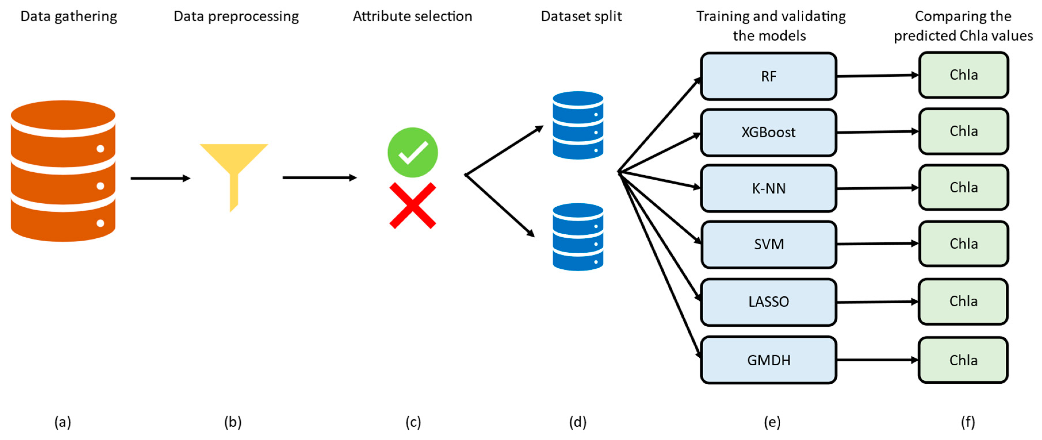
2.4. Machine Learning Models

In this study, Chla was estimated using satellite data and machine learning models. The first implemented approach was a random forest (RF) model. An RF model is a model of trees trained using the bagging method of resampling while considering only a subset of predictors (Figure 2 and Figure 3) [88,89], making it an ensemble model. The trained trees have a low correlation, thus reducing the ensemble model variance and improving performance [90]. A number of published works have investigated the RF methodology [91,92,93].

XGBoost [94] is tree-based approach that is also an ensemble model, representing an extreme improvement over the random forest approach. It consists of bag sampling smaller tree models to combine them into a larger and more robust tree model, thereby reducing the model variance while improving its generalization and reducing the tendency to overfit [90,95]. The XGBoost approach can handle missing data and manipulate increasing dataset size, thus maintaining its generalization. This approach has been reported to reach excellent results when applied to different time series forecasting tasks [84,96,97].

K-nearest neighbors (k-NN) is a supervised ML model that uses non-parametric vectors to determine an unknown point, which can be applied to data classification and regression cases [85,98]. Despite its simplicity, the regression performed by the k-NN approach offers competitive results within the ML field and has been explored for different scenarios in previous studies [99,100,101].

Support vector machine (SVM) is a flexible ML approach with diverse applications in classification, regression, and outlier detection [102]. A unique feature of SVM is the use of kernel functions that allow a dataset to be transformed into higher-dimensional spaces, making it possible for the model to learn complex non-linear relationships by applying convex optimization without being computationally expensive, thus reducing the training error [98,103,104]. However, one drawback of the SVM approach is that it does not handle large datasets efficiently as it requires extended computational time to be trained [105,106].

The least absolute shrinkage and selection operator (LASSO) regression [107] was another ML methodology implemented in this study. This approach is a more straightforward ML methodology that seeks to implement the best linear regression to a dataset. In addition to that, the LASSO paradigm is also a regularization and parameter selection approach, making its results more interpretable than other traditional ML models [90,107].

Lastly, we investigated the application of the GMDH ML model for Chla modeling using satellite data. This methodology is a feedforward unidirectional ML model, similar to a multilayer perceptron [108,109]. It is a self-organizing model whose parameters are selected automatically without the need for tuning [110]. The resulting value obtained by the GMDH model is a quadratic approximation, using pair combinations of the input variables [111,112] to model the relationship between the input and output parameters [113]. Unlike other artificial neural network paradigms, the GMDH model does not need large amounts of training data, as the estimation of its parameters is automatically determined without recursion [20]. The performance of the GMDH model has been verified in previous studies for time series challenges, including hydrological applications [114,115,116].

2.5. Evaluation Metrics

To assess the forecast performance of the proposed models, we opted to calculate the root mean squared error (RMSE), normalized RMSE (nRMSE), mean absolute error (MAE), mean absolute percentage error (MAPE), mean bias error (MBE), and coefficient of determination (R²). The equation for R² can be found in [117], and the equations for the remaining metrics can be found in [118].

2.6. Dataset Preprocessing and Attribute Selection

Dataset standardization is a technique that rescales the features within a dataset to a common scale, typically by setting the mean to zero and the standard deviation to one. This can improve the performance of some machine learning models [119]. In addition to data standardization, the Yeo–Johnson transformation [120] was implemented in this study for some of the ML models. This transformation is an improvement over the Box–Cox approach, which is restricted to handling positive numbers only. The Yeo–Johnson transformation is based on the power transformation of different parameters to positive and negative values and is presented in Equation (18) [120]:

$$\psi \left(y,\mathsf{\lambda }\right)=\left\{\begin{array}{ll}\frac{(y+1{)}^{\lambda }+1}{\lambda }& y\ge 0,\lambda \ne 0\\ \log \left(y+1\right)& y\ge 0,\lambda =0\\ -\frac{(-y+1{)}^{2-\lambda }-1}{2-\lambda }& y<0,\lambda \ne 2\\ -\log \left(-y+1\right)& y<0,\lambda =2\end{array}\right.$$

(17)

where the transformed value ψ is a function of the original attribute value, $y$, and a parameter $\lambda$, which is determined via maximum likelihood. This transformation seeks to reduce data skewness by approximating the original dataset distribution to a normal distribution as $\psi \left(y,\lambda \right) \sim N\left(\mu , {\sigma }^2\right)$ [121,122].

To select the most relevant features for the models, a step-by-step approach was implemented [85]. We began by investigating the influence of the individual bands 1 to 12, using the XGBoost model as a benchmark. The choice of XGBoost was motivated because it is a state-of-the-art model well known for its robustness and for providing excellent outcomes [119,123]. The band that returned the best R² was chosen. After that, we tested the combination of the selected feature with the remaining bands, one by one, and kept the band combination that returned the highest coefficient of determination. This process continued until all bands were evaluated, and the combination that yielded the best overall performance was identified [85]. A visual illustration of this process is depicted in Figure 4 for the selection of the most informative spectral bands.

The same procedure was repeated for the selection of the indices. This time, we started the investigation with the best band that was previously selected. Then, we added one index at a time to the input parameters and selected the index that yielded the highest R². This process was repeated until all the indices were assessed. The selections of the best bands and indices are presented in Figure 5 and Figure 6, respectively.

As depicted in Figure 5, the modeling for Chla detection substantially improved with the combination of bands 6, 4, 10, 7, 8A, 9, 5, 12, and 3, achieving an R² of 0.36. Figure 6 shows that incorporating additional indices, namely NBRI, NDSI, AWEI, SAVI, NDVI, MSI, GCI, GNDVI, and ARVI, further increased the coefficient of determination to 0.50. Interestingly, including the NDSI, an index related to snow coverage, improved the Chla identification, as shown in Figure 5. This suggests that the NDSI conveys valuable spatiotemporal information for the modeling approach. Therefore, the results discussed in the subsequent section are based on grouping the aforementioned spectral bands and indices.

Figure 7 summarizes the proposed methodology of this study. It depicts a step-by-step process, from acquiring data (a) to evaluating the performance of various machine learning models (f).

3. Results

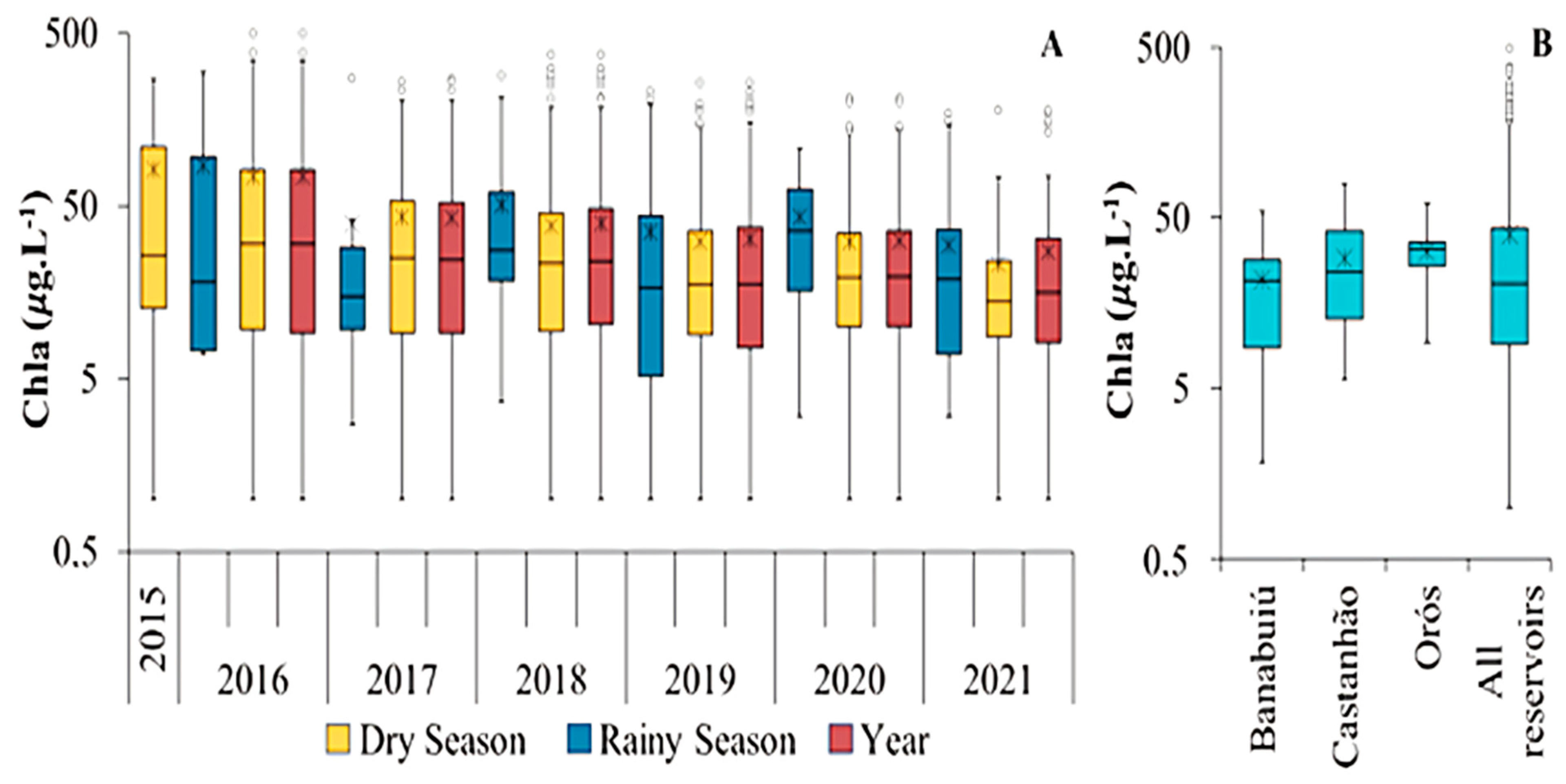
3.1. Limnological Behavior

The mean values for chlorophyll-a varied significantly across the reservoirs and according to seasonality. Considering the entire dataset, Chla ranged from 1 μg/L to 1001.78 μg/L, with an average of 39.62 μg/L and a standard deviation of 65.78 μg/L. Figure 8A shows the distribution of Chla concentrations across years and seasons. The mean values decreased over the years (from 81.34 μg/L in 2015 to 27.84 μg/L in 2021), while the maximum values did not follow this trend, showing occasional spikes with values ranging from 707.06 in 2015 to 1001.78 in 2016. This indicated periods of concentrated blooms. Regarding the seasonal distribution of Chla, higher concentrations were detected during the rainy seasons for most of the studied years, except in 2017.

Figure 8B shows the Chla concentrations in the state’s three largest reservoirs. Orós had the highest recorded average, at 31.89 μg/L, with a range from 9.20 to 60.94 μg/L. The mean Chla concentration for Banabuiú was the lowest recorded, at 21.64 μg/L, fluctuating between 1.82 and 54.55 μg/L. Lastly, the values for Castanhão ranged from 5.65 to 78.72 μg/L, with the second highest mean Chla value of 29.03 μg/L.

3.2. Results of Chla Concentrations Estimated by the ML Models

The proposed models were built using the variables presented in Figure 5 and Figure 6 as the input parameters. We used data from the Sentinel-2 satellite and on-site measurements from the 149 reservoirs to train and test these models. We adopted a 70/30 split for the training and validation datasets, which were randomly assembled using data from 2015 to 2021. It is important to note that given the random sampling for the training and validation datasets, not all reservoirs might have been included in the validation dataset. However, this does not mean that the validation dataset does not have statistical characteristics similar to the training dataset.

The models were implemented in Python language, version 3.11.7. The hyperparameters of the tested ML models, except for the GMDH self-organizing model, were selected using the GridSearch tool from Scikit-Learn version 1.2.2, with fivefold cross-validation [124,125]. The outcomes of Chla modeling by each of the assessed models are presented in

Table 2. Results of Chla concentrations estimated by the models.

Model	RMSE (μg/L)	nRMSE (%)	MAE (μg/L)	MAPE (%)	MBE (μg/L)	R2	Yeo–Johnson Transformation
k-NN	61.82	146.07	30.90	260.60	−4.91	0.38	Yes
XGBoost	55.60	131.36	29.41	288.34	−2.53	0.50	No
RF	56.75	134.10	29.92	311.58	−1.54	0.48	No
SVR	50.64	119.64	25.07	182.60	−6.97	0.58	Yes
LASSO	89.87	212.34	47.41	466.35	−3.60	0.41	Yes
GMDH	20.38	53.20	14.09	102.34	−4.86	0.91	Yes

.

Table 2 shows that the ML models reached similar results regarding the RMSE metric, except for the GMDH model, which surpassed all other models, achieving an RMSE of 20.38 μg/L and an R² of 91%. The LASSO model achieved the highest value of RMSE, at 89.87 μg/L, followed by the k-NN model, with an RMSE value of 61.82 μg/L. The tree-based XGBoost and RF models achieved similar RMSE values of 55.60 μg/L and 56.75 μg/L, respectively. The SVR output scored an RMSE value equal to 50.64 μg/L. It is essential to note that an analysis of the RMSE alone may be misleading when assessing the performance of models. The coefficient of determination is another crucial factor to consider in this scenario. This parameter indicates the total variance in the dependent variable Chla, which can be adequately forecasted by the input parameters and may be viewed as an indication of the accuracy achieved by a model [126]. This behavior can be better visualized by examining Figure 8.

Figure 9 shows how the predicted data compare with the measured Chla values. We used log values to facilitate the comparison due to differences in the variables’ scales. The histograms show the normal distribution of the data after the logarithm transformation. In Figure 9, given the log scale, minor fluctuations in Chla values correspond to negligible alterations in the satellite-captured data. This is not related to the GMDH model itself but is a consequence of the chosen scale. The use of remote sensing data lacks the sensibility to convey sufficient information at low Chla values, since a main characteristic of high Chla concentrations is their tendency to converge to a specific spectral pattern that appears green, while at low values, they tend to converge to different spectral patterns depending on the characteristics of each reservoir.

However, in Figure 9, it is still possible to observe that both the predicted and measured data present similar distributions, which indicates the GMDH model’s good performance in predicting Chla levels. The regression line displayed in the plotting area shows a positive correlation between the predicted and measured Chla data, further attesting to the robust performance of the GMDH model. The points clustered around the regression line also indicate the superior performance of the GMDH model, especially for extreme values, as depicted by the top-rightmost points in the graph area. Comparing the results in Table 2, we can see that the highest R² value reached by the GMDH model was 0.91, representing a significant improvement of 57% over the SVR result, the second-best-performing model regarding the same parameter. The third- and fourth-best-performing models were the tree-based XGBoost and RF models, which achieved R² values equal to 0.50 and 0.48, respectively.

Regarding the performance of the k-NN model, the R² was 0.38, and for the LASSO model, the R² was 0.38 and the coefficient of determination was 0.41, indicating it was the worst-performing modeling paradigm. An analysis of the values of MAE and MAPE indicated that the GMDH model could output more accurate and precise results compared to the other assessed models. The negative values of MBE were a trend present in all of the investigated models. This result indicates that the ML models share the tendency to underestimate the Chla values.

4. Discussion

Advanced analysis is required to understand the mechanisms that regulate phytoplankton growth in tropical regions due to the complexity and non-linearity of the relationship between chlorophyll and physicochemical/environmental factors [24,127]. The approach presented in this study achieved such an analysis by using a highly heterogeneous collection of in situ observations and investigating the performance of different ML models in determining the Chla levels in 149 reservoirs in the Brazilian state of Ceará. Although most reservoirs are predominantly eutrophic throughout the years, various human activities and pollution sources have contributed to the eutrophication processes, leading to Chla spatiotemporal fluctuations and algal blooms [30,34,128,129].

4.1. Parameter Selection

We applied the forward stepwise approach to select the parameters, including bands and spectral indices. To the best of our knowledge, this method has not yet been applied in previous remote sensing studies. The forward stepwise approach significantly improved the accuracy of the ML models in determining the Chla levels. Existing literature regarding the influence of spectral bands on Chla determination can be found. In [130], the authors applied the SHAP analysis to determine the influence of the Sentinel-2 spectral bands on the estimation of Chla values. Their results showed that bands 2, 3, and 8 were the top three most influential parameters for Chla determination. Bands 2 and 3 exhibited a positive correlation with the Chla value, while band 8 showed a negative correlation with the same parameter. A similar approach was conducted by Kim et al. [131]. In their work, the SHAP analysis showed the participation of red bands, i.e., bands 4, 5, and 6, as well as blue and green bands in Chla prediction (Table 1). A similar conclusion was reported by Ha et al. [132].

The influence of different spectral indices on Chla modeling has been investigated in previous works. Castro et al. [133] showed that indices merging red and NIR bands yielded the best outcomes for determining Chla concentrations in small reservoirs. Similar conclusions were drawn by Buma and Lee [134] and Aubriot et al. [135], who confirmed the importance of bands within the red spectral range for Chla characterization in a lake in Chad and the Rio de La Plata, respectively. On the other hand, Viso-Vazquez et al. [136] showed that a green band, i.e., band 3, contributed the most to the correlation between the remote sensing data and Chla levels.

4.2. ML Model Comparison

The “no free lunch theorem” states that no single best machine learning model exists for every task [137]. In fact, different models will perform differently on the same task under the same conditions, and one of the models may achieve better outcomes compared to the others. In this case, the proposed GMDH model was the best-performing approach. The GMDH model has also been found to achieve excellent results in time series hydrological applications, which could, in part, justify its superior results [108,138].

Our results show the GMDH approach could efficiently identify the latent non-linear ties influencing the input and output attributes. The GMDH approach proved to be a more robust model for analyzing satellite imagery as it was more resilient to noise. Additionally, it provided satisfactory results in handling different band information. Therefore, given its simple implementation and superior performance, the GMDH model poses as a strong contender for a real-time Chla monitoring tool.

4.3. Comparison with Previous Works

To better understand where the GMDH results lie within the literature, we compared our results with those found in previously published works. Such an evaluation, however, may not be representative given the different methodologies, models, and input attributes used in different studies, as well as the different study areas. Yet, comparing their evaluation metrics is still a viable approach for assessing the performance of different models [139].

Table 3. Results of the GMDH model’s estimation of Chla levels.

Model	RMSE (μg/L)	MAE (μg/L)	MBE (μg/L)	MAPE (%)	R2
GMDH	20.38	14.09	−4.86	102.34	0.91

presents the results of the GMDH model, while

Table 4. Compilation of results of Chla modeling found in the literature.

Model	Location	Dataset	RMSE μg/L	R2	Reference
Multimodal Deep Learning	Lake Simcoe, Canada	Sentinel-2 and Landsat-8 imagery	60	0.92	[140]
Convolutional Neural Network	Lake Balik, Turkey	Sentinel-2 imagery	2.9	0.95	[141]
Convolutional Neural Network	11 lakes in Karlsruhe, Germany	Simulated Chla data used for training, data from SpecWa used for evaluation	12.4	0.82	[142]
SVR	45 lakes across China	Sentinel-2 imagery	6.3	0.88	[143]
SVR	Buffalo Pound Lake, Canada	Sentinel-2 imagery	13.9	0.66	[144]
Toming’s Index	A Baxe reservoir, Spain	Sentinel-2 imagery	-	0.86	[136]
3BSI Index	5 reservoirs in Ceará, Brazil	Sentinel-2 imagery	-	0.80	[24]
C2RCC Atmospheric Correction	6 reservoirs in São Paulo, Brazil	Sentinel-2 imagery	2.3	0.75	[145]

presents the results found in the literature.

Table 4 shows that the models based on the deep learning methodology all performed remarkably well in determining Chla levels. Compared to the results found in our study, it is noted that the R-squared values reported in references [140,141] are in the same range, over 90%. Nevertheless, in the work by Guo et al. [140], the combined utilization of Sentinel-2 and Landsat-8 data significantly enhanced the machine learning model’s performance. This improvement was primarily due to the reduction in revisit time, which subsequently minimized the variance in the dataset. Consequently, this led to a more robust and accurate machine learning model. It is important to note that, although the results were slightly superior in that work, the study location was limited to only one site.

Adding data from more water bodies is expected to add variance to the dataset. The model in reference [142] was built using simulated data from 11 times more water bodies than the previous studies. The results proved slightly inferior to the other two previous works and were closer to the values found in the present assessment, with the RMSE in the same order of magnitude.

Regarding the R², our GMDH model showed a nearly 10% superior value. However, it must be noted that since the data used for training the ML model were simulated, the authors of [142] might not have considered several naturally occurring situations. This would lead to a more homogeneous dataset with less variance, thus improving the ML model performance compared to the model proposed in our study. Another significant difference is the time window used for testing the developed model in reference [142], which was significantly smaller than the one used in our model [146]; this also reduced the dataset variance, thereby improving the ML model performance.

The DL approaches presented in Table 4 require considerable amounts of data to yield reliable outputs. Depending on the data availability for a study location, this characteristic may pose a major drawback. On the other hand, the GMDH approach can be promptly implemented with less information available and does not require extensive training datasets, making it more flexible for different situations.

The authors of [143,144] applied SVR to determine the Chla levels. It is noticeable that although the models were the same, their methodology was different. Regarding reference [143], the RMSE values were within the same order of magnitude and the R² values were relatively close to each other. In contrast, the authors of [144] performed a much broader study on several lakes spread across the Chinese territory. As previously mentioned, including a greater number of lakes allows the forecasting model to better generalize its results, thus providing more robust outcomes. Another critical difference between these two works is that the former implemented only the spectral bands of the MSI on board Sentinel-2 as the input information, while the latter used both bands and indices. In this respect, the present study achieved superior performance, attesting that the GMDH model benefited from the inclusion of spectral indices, which improved the Chla values.

The work conducted by Aranha et al. [24] shared the same location as the one used in this study. However, they used only a subset of 5 reservoirs out of 149. In their approach, the authors fitted a regression line to their dataset using the three-band spectral index (3BSI), showing good agreement between the index and the Chla values. A similar methodology was implemented in reference [136], where the Toming’s index was used to fit a regression line for the Chla values. These two studies implemented spectral bands to estimate Chla concentrations. By evaluating the R² metric values in [24,136], the proposed GMDH model was superior to the models used in both studies, with significant improvements of 12% and 5%, respectively. Furthermore, a major difference in methodology between these two studies and the present work was data handling. The other studies proceeded to fit a regression line using the proposed indices over the entire dataset, making no distinction between training and testing datasets. This would be analogous to assessing our ML model’s performance considering the training dataset only. Therefore, their methodologies lacked generalization, being bound to a particular time and geographic location. Nevertheless, while these approaches were considerably less complex than the proposed ML model, they provided valuable insights into Chla’s behavior when analyzed using the evaluated indices.

In the work conducted by Pompêo et al. [145], the Sentinel application platform (SNAP) algorithm was used to model the Secchi disk depth, Chla concentration, and number of cyanobacteria cells. The study location was the Cantareira System (CS) in the Brazilian state of São Paulo, Brazil. The authors used in situ collected water samples from six reservoirs in the CS as ground truth for the evaluation of water quality parameters. These data were later compared with the data obtained using the case-2 regional coast color (C2RCC) atmospheric correction algorithm. This is a machine learning paradigm based on neural networks trained to reproduce top-of-atmosphere reflectance [147]. The results of their study showed a good correlation between the modeled data and the real collected sample data for Chla, achieving an RMSE value of 2.3 μg/L and an R² of 0.75.

A direct comparison of these results with the ones found in our study showed an R-squared value that was 16% superior for the GMDH approach, while the C2RCC had better RMSE values. The reason behind this discrepancy for the error metrics is twofold. First, even though both studies were conducted in the Brazilian territory, the state of São Paulo is characterized by a subtropical and tropical climate type [148]. Such a climatic configuration is much less prone to dry seasons compared to the studied semi-arid region of the Ceará state. This leads to less fluctuation in Chla levels. Consequently, this could decrease the model’s variance, thus enhancing its performance. Second, the work presented by Pompêo et al. used significantly fewer reservoirs compared to the present work. As previously mentioned, a reduced number of reservoirs hinders a model’s capacity to generalize to unknown data while diminishing the dataset’s variance, leading to improved error outcomes. However, despite the improved error, the C2RCC model is a less robust approach when compared to the GMDH model, as evidenced in the comparison of the R² metrics of the two models.

4.4. Most Relevant Spectral Bands

A comprehensive investigation of the spectral indices from the Sentinel-2 constellation allowed us to gain deeper insights into the spatiotemporal influence of both bands and indices on Chla prediction. Our results from parameter selection (Figure 5 and Figure 6) show that while bands 8 and 11 were not part of the selected band set, they were still present in the form of indices. A detailed review of the GMDH results (available in Supplementary Spreadsheet 1) highlights the significant contribution of bands 3, 4, 5, 7, 8, and 11 to Chla prediction. This suggests that the proposed model benefits from a higher spatial resolution and the inclusion of green, red, and infrared bands in the indices, which aligns with the existing literature [13,24,52].

5. Conclusions

This study evaluated several input parameters for Chla modeling using data from 149 freshwater reservoirs that span a vast semi-arid tropical region across the Brazilian state of Ceará. This assessment was conducted using satellite remote sensing data and ground-truth Chla measurements, reflecting the temporal and spatial distributions, which were notably impacted by interannual rainfall variability. To this end, we investigated the performance of several ML approaches using forward stepwise parameter selection. From the obtained results, we can make the following conclusions:

• Using forward stepwise selection, a new approach in the remote sensing field, succeeded in improving Chla modeling by selecting input parameters that consisted of both spectral bands and indices.
• Proper separation between training and testing datasets, which is usually overlooked in similar works, improved model generalization, as demonstrated by the models’ results in Table 2.
• The best-performing model was the GMDH model, achieving an R² value of 91%, a significant improvement over the results obtained by the other assessed models. This superior performance shows that this approach is suitable for Chla modeling using remote sensing data.
• Chla modeling benefited most from the inclusion of the red, NIR, and green bands, specifically bands 3, 4, 5, 7, 8, and 11.
• An extensive comparison with previous studies showed that the models tested in this work offered competitive results.

In future works, the inclusion of more spectral indices and the Landsat-8 MODIS data would provide more spatiotemporal information and reduce data variance due to the finer temporal resolution. Furthermore, implementing atmospheric correction preprocessing could also benefit the predictive paradigms being evaluated, as it would reduce data noise, diminish the error variance, and improve the forecasting of Chla concentrations. Finally, understanding how dataset size influences uncertainty in deep learning models could be crucial for optimizing their performance in this specific application.

References

1. Kayastha, P.; Dzialowski, A.R.; Stoodley, S.H.; Wagner, K.L.; Mansaray, A.S. Effect of Time Window on Satellite and Ground-Based Data for Estimating Chlorophyll-a in Reservoirs. Remote Sens. 2022, 14, 846. [Google Scholar] [CrossRef]
2. Zhu, W.-D.; Qian, C.-Y.; He, N.-Y.; Kong, Y.-X.; Zou, Z.-Y.; Li, Y.-W. Research on Chlorophyll-a Concentration Retrieval Based on BP Neural Network Model—Case Study of Dianshan Lake, China. Sustainability 2022, 14, 8894. [Google Scholar] [CrossRef]
3. Cao, Z.; Ma, R.; Duan, H.; Pahlevan, N.; Melack, J.; Shen, M.; Xue, K. A Machine Learning Approach to Estimate Chlorophyll-a from Landsat-8 Measurements in Inland Lakes. Remote Sens. Environ. 2020, 248, 111974. [Google Scholar] [CrossRef]
4. Fu, L.; Zhou, Y.; Liu, G.; Song, K.; Tao, H.; Zhao, F.; Li, S.; Shi, S.; Shang, Y. Retrieval of Chla Concentrations in Lake Xingkai Using OLCI Images. Remote Sens. 2023, 15, 3809. [Google Scholar] [CrossRef]
5. Dzurume, T.; Dube, T.; Shoko, C. Remotely Sensed Data for Estimating Chlorophyll-a Concentration in Wetlands Located in the Limpopo Transboundary River Basin, South Africa. Phys. Chem. Earth Parts A/B/C 2022, 127, 103193. [Google Scholar] [CrossRef]
6. Karimian, H.; Huang, J.; Chen, Y.; Wang, Z.; Huang, J. A Novel Framework to Predict Chlorophyll-a Concentrations in Water Bodies through Multi-Source Big Data and Machine Learning Algorithms. Environ. Sci. Pollut. Res. 2023, 30, 79402–79422. [Google Scholar] [CrossRef] [PubMed]
7. Zhang, X.; Chen, X.; Zheng, G.; Cao, G. Improved Prediction of Chlorophyll-a Concentrations in Reservoirs by GRU Neural Network Based on Particle Swarm Algorithm Optimized Variational Modal Decomposition. Environ. Res. 2023, 221, 115259. [Google Scholar] [CrossRef] [PubMed]
8. Li, J.; Pei, Y.; Zhao, S.; Xiao, R.; Sang, X.; Zhang, C. A Review of Remote Sensing for Environmental Monitoring in China. Remote Sens. 2020, 12, 1130. [Google Scholar] [CrossRef]
9. Pahlevan, N.; Smith, B.; Schalles, J.; Binding, C.; Cao, Z.; Ma, R.; Alikas, K.; Kangro, K.; Gurlin, D.; Hà, N.; et al. Seamless Retrievals of Chlorophyll-a from Sentinel-2 (MSI) and Sentinel-3 (OLCI) in Inland and Coastal Waters: A Machine-Learning Approach. Remote Sens. Environ. 2020, 240, 111604. [Google Scholar] [CrossRef]
10. Song, K.; Wang, Q.; Liu, G.; Jacinthe, P.-A.; Li, S.; Tao, H.; Du, Y.; Wen, Z.; Wang, X.; Guo, W.; et al. A Unified Model for High Resolution Mapping of Global Lake (>1 Ha) Clarity Using Landsat Imagery Data. Sci. Total Environ. 2022, 810, 151188. [Google Scholar] [CrossRef] [PubMed]
11. Shi, J.; Shen, Q.; Yao, Y.; Li, J.; Chen, F.; Wang, R.; Xu, W.; Gao, Z.; Wang, L.; Zhou, Y. Estimation of Chlorophyll-a Concentrations in Small Water Bodies: Comparison of Fused Gaofen-6 and Sentinel-2 Sensors. Remote Sens. 2022, 14, 229. [Google Scholar] [CrossRef]
12. Segarra, J.; Buchaillot, M.L.; Araus, J.L.; Kefauver, S.C. Remote Sensing for Precision Agriculture: Sentinel-2 Improved Features and Applications. Agronomy 2020, 10, 641. [Google Scholar] [CrossRef]
13. Bramich, J.; Bolch, C.J.S.; Fischer, A. Improved Red-Edge Chlorophyll-a Detection for Sentinel 2. Ecol. Indic. 2021, 120, 106876. [Google Scholar] [CrossRef]
14. Oliveira Santos, V.; Costa Rocha, P.A.; Thé, J.V.G.; Gharabaghi, B. Graph-Based Deep Learning Model for Forecasting Chloride Concentration in Urban Streams to Protect Salt-Vulnerable Areas. Environments 2023, 10, 157. [Google Scholar] [CrossRef]
15. Oliveira Santos, V.; Costa Rocha, P.A.; Scott, J.; Van Griensven Thé, J.; Gharabaghi, B. Spatiotemporal Air Pollution Forecasting in Houston-TX: A Case Study for Ozone Using Deep Graph Neural Networks. Atmosphere 2023, 14, 308. [Google Scholar] [CrossRef]
16. Hieronymi, M.; Müller, D.; Doerffer, R. The OLCI Neural Network Swarm (ONNS): A Bio-Geo-Optical Algorithm for Open Ocean and Coastal Waters. Front. Mar. Sci. 2017, 4, 140. [Google Scholar] [CrossRef]
17. Moutzouris-Sidiris, I.; Topouzelis, K. Assessment of Chlorophyll-a Concentration from Sentinel-3 Satellite Images at the Mediterranean Sea Using CMEMS Open Source In Situ Data. Open Geosci. 2021, 13, 85–97. [Google Scholar] [CrossRef]
18. Shi, X.; Gu, L.; Jiang, T.; Zheng, X.; Dong, W.; Tao, Z. Retrieval of Chlorophyll-a Concentrations Using Sentinel-2 MSI Imagery in Lake Chagan Based on Assessments with Machine Learning Models. Remote Sens. 2022, 14, 4924. [Google Scholar] [CrossRef]
19. Hu, C.; Feng, L.; Guan, Q. A Machine Learning Approach to Estimate Surface Chlorophyll a Concentrations in Global Oceans From Satellite Measurements. IEEE Trans. Geosci. Remote Sens. 2021, 59, 4590–4607. [Google Scholar] [CrossRef]
20. Alizamir, M.; Heddam, S.; Kim, S.; Mehr, A.D. On the Implementation of a Novel Data-Intelligence Model Based on Extreme Learning Machine Optimized by Bat Algorithm for Estimating Daily Chlorophyll-a Concentration: Case Studies of River and Lake in USA. J. Clean. Prod. 2021, 285, 124868. [Google Scholar] [CrossRef]
21. Loc, H.H.; Do, Q.H.; Cokro, A.A.; Irvine, K.N. Deep Neural Network Analyses of Water Quality Time Series Associated with Water Sensitive Urban Design (WSUD) Features. J. Appl. Water Eng. Res. 2020, 8, 313–332. [Google Scholar] [CrossRef]
22. Chen, J.; Yin, H.; Zhang, D. A Self-Adaptive Classification Method for Plant Disease Detection Using GMDH-Logistic Model. Sustain. Comput. Inform. Syst. 2020, 28, 100415. [Google Scholar] [CrossRef]
23. Beck, H.E.; Zimmermann, N.E.; McVicar, T.R.; Vergopolan, N.; Berg, A.; Wood, E.F. Present and Future Köppen-Geiger Climate Classification Maps at 1-Km Resolution. Sci. Data 2018, 5, 180214. [Google Scholar] [CrossRef]
24. Aranha, T.R.B.T.; Martinez, J.-M.; Souza, E.P.; Barros, M.U.G.; Martins, E.S.P.R. Remote Analysis of the Chlorophyll-a Concentration Using Sentinel-2 MSI Images in a Semiarid Environment in Northeastern Brazil. Water 2022, 14, 451. [Google Scholar] [CrossRef]
25. do Sacramento, E.M.; Carvalho, P.C.M.; de Araújo, J.C.; Riffel, D.B.; Corrêa, R.M. da C.; Pinheiro Neto, J.S. Scenarios for Use of Floating Photovoltaic Plants in Brazilian Reservoirs. IET Renew. Power Gener. 2015, 9, 1019–1024. [Google Scholar] [CrossRef]
26. INSA O Semiárido Brasileiro. Available online: https://www.gov.br/insa/pt-br/semiarido-brasileiro/o-semiarido-brasileiro (accessed on 1 December 2023).
27. Barros, M.U.G.; Wilson, A.E.; Leitão, J.I.R.; Pereira, S.P.; Buley, R.P.; Fernandez-Figueroa, E.G.; Capelo-Neto, J. Environmental Factors Associated with Toxic Cyanobacterial Blooms across 20 Drinking Water Reservoirs in a Semi-Arid Region of Brazil. Harmful Algae 2019, 86, 128–137. [Google Scholar] [CrossRef]
28. Lu, K.; Gao, X.; Yang, F.; Gao, H.; Yan, X.; Yu, H. Driving Mechanism of Water Replenishment on DOM Composition and Eutrophic Status Changes of Lake in Arid and Semi-Arid Regions of Loess Area. Sci. Total Environ. 2023, 899, 165609. [Google Scholar] [CrossRef]
29. Raulino, J.B.S.; Silveira, C.S.; Lima Neto, I.E. Assessment of Climate Change Impacts on Hydrology and Water Quality of Large Semi-Arid Reservoirs in Brazil. Hydrol. Sci. J. 2021, 66, 1321–1336. [Google Scholar] [CrossRef]
30. Guimarães, B.M.D.M.; Neto, I.E.L. Chlorophyll-a Prediction in Tropical Reservoirs as a Function of Hydroclimatic Variability and Water Quality. Environ. Sci. Pollut. Res. 2023, 30, 91028–91045. [Google Scholar] [CrossRef] [PubMed]
31. Rocha Junior, C.A.N.D.; Costa, M.R.A.D.; Menezes, R.F.; Attayde, J.L.; Becker, V. Water Volume Reduction Increases Eutrophication Risk in Tropical Semi-Arid Reservoirs. Acta Limnol. Bras. 2018, 30, e106. [Google Scholar] [CrossRef]
32. Rocha, M.D.J.D.; Lima Neto, I.E. Modeling Flow-Related Phosphorus Inputs to Tropical Semiarid Reservoirs. J. Environ. Manag. 2021, 295, 113123. [Google Scholar] [CrossRef]
33. Rocha, M.D.J.D.; Lima Neto, I.E. Internal Phosphorus Loading and Its Driving Factors in the Dry Period of Brazilian Semiarid Reservoirs. J. Environ. Manag. 2022, 312, 114983. [Google Scholar] [CrossRef]
34. Wiegand, M.C.; Do Nascimento, A.T.P.; Costa, A.C.; Lima Neto, I.E. Trophic State Changes of Semi-Arid Reservoirs as a Function of the Hydro-Climatic Variability. J. Arid Environ. 2021, 184, 104321. [Google Scholar] [CrossRef]
35. COGERH Matriz Dos Usos Mútiplos Dos Açudes. Available online: http://www.hidro.ce.gov.br/hidro-ce-zend/mi/midia/show/149 (accessed on 1 December 2023).
36. Freire, L.L.; Costa, A.C.; Neto, I.E.L. Effects of Rainfall and Land Use on Nutrient Responses in Rivers in the Brazilian Semiarid Region. Environ. Monit. Assess. 2023, 195, 652. [Google Scholar] [CrossRef]
37. Rabelo, U.P.; Dietrich, J.; Costa, A.C.; Simshäuser, M.N.; Scholz, F.E.; Nguyen, V.T.; Lima Neto, I.E. Representing a Dense Network of Ponds and Reservoirs in a Semi-Distributed Dryland Catchment Model. J. Hydrol. 2021, 603, 127103. [Google Scholar] [CrossRef]
38. Rabelo, U.P.; Costa, A.C.; Dietrich, J.; Fallah-Mehdipour, E.; Van Oel, P.; Lima Neto, I.E. Impact of Dense Networks of Reservoirs on Streamflows at Dryland Catchments. Sustainability 2022, 14, 14117. [Google Scholar] [CrossRef]
39. IBGE Ceará|Cidades e Estados|IBGE. Available online: https://www.ibge.gov.br/cidades-e-estados/ce.html (accessed on 1 December 2023).
40. COGERH Portal Hidrológico Do Ceará. Available online: http://www.hidro.ce.gov.br/ (accessed on 1 December 2023).
41. American Public Health Association; American Water Works Association; Water Environment Federation (Eds.) Standard Methods for the Examination of Water and Wastewater, 22nd ed.; American Public Health Association: Washington, DC, USA, 2012; ISBN 978-0-87553-013-0. [Google Scholar]
42. Phiri, D.; Simwanda, M.; Salekin, S.; Nyirenda, V.; Murayama, Y.; Ranagalage, M. Sentinel-2 Data for Land Cover/Use Mapping: A Review. Remote Sens. 2020, 12, 2291. [Google Scholar] [CrossRef]
43. Drusch, M.; Del Bello, U.; Carlier, S.; Colin, O.; Fernandez, V.; Gascon, F.; Hoersch, B.; Isola, C.; Laberinti, P.; Martimort, P.; et al. Sentinel-2: ESA’s Optical High-Resolution Mission for GMES Operational Services. Remote Sens. Environ. 2012, 120, 25–36. [Google Scholar] [CrossRef]
44. Zhang, T.; Su, J.; Liu, C.; Chen, W.-H.; Liu, H.; Liu, G. Band Selection in Sentinel-2 Satellite for Agriculture Applications. In Proceedings of the 2017 23rd International Conference on Automation and Computing (ICAC), Huddersfield, UK, 7–8 September 2017; IEEE: Piscataway, NJ, USA, 2017; pp. 1–6. [Google Scholar]
45. Ienco, D.; Interdonato, R.; Gaetano, R.; Ho Tong Minh, D. Combining Sentinel-1 and Sentinel-2 Satellite Image Time Series for Land Cover Mapping via a Multi-Source Deep Learning Architecture. ISPRS J. Photogramm. Remote Sens. 2019, 158, 11–22. [Google Scholar] [CrossRef]
46. Zhang, T.-X.; Su, J.-Y.; Liu, C.-J.; Chen, W.-H. Potential Bands of Sentinel-2A Satellite for Classification Problems in Precision Agriculture. Int. J. Autom. Comput. 2019, 16, 16–26. [Google Scholar] [CrossRef]
47. Ma, Y.; Xu, N.; Liu, Z.; Yang, B.; Yang, F.; Wang, X.H.; Li, S. Satellite-Derived Bathymetry Using the ICESat-2 Lidar and Sentinel-2 Imagery Datasets. Remote Sens. Environ. 2020, 250, 112047. [Google Scholar] [CrossRef]
48. European Space Agency User Guides—Sentinel-2 MSI—Level-1C Product—Sentinel Online. Available online: https://copernicus.eu/user-guides/sentinel-2-msi/product-types/level-1c (accessed on 3 February 2024).
49. European Space Agency Sentinel-2 MSI Level-1C TOA Reflectance. Available online: https://sentinels.copernicus.eu/web/sentinel/sentinel-data-access/sentinel-products/sentinel-2-data-products/collection-1-level-1c (accessed on 3 February 2024).
50. European Space Agency Annual Performance Report. Available online: https://sentinels.copernicus.eu/web/sentinel/technical-guides/sentinel-2-msi/data-quality-reports (accessed on 3 February 2024).
51. Prasad, A.D.; Ganasala, P.; Hernández-Guzmán, R.; Fathian, F. Remote Sensing Satellite Data and Spectral Indices: An Initial Evaluation for the Sustainable Development of an Urban Area. Sustain. Water Resour. Manag. 2022, 8, 19. [Google Scholar] [CrossRef]
52. Gitelson, A. The Peak near 700 Nm on Radiance Spectra of Algae and Water: Relationships of Its Magnitude and Position with Chlorophyll Concentration. Int. J. Remote Sens. 1992, 13, 3367–3373. [Google Scholar] [CrossRef]
53. Hamunzala, B.; Matsumoto, K.; Nagai, K. Improved Method for Estimating Construction Year of Road Bridges by Analyzing Landsat Normalized Difference Water Index 2. Remote Sens. 2023, 15, 3488. [Google Scholar] [CrossRef]
54. Abd El-Sadek, E.; Elbeih, S.; Negm, A. Coastal and Landuse Changes of Burullus Lake, Egypt: A Comparison Using Landsat and Sentinel-2 Satellite Images. Egypt. J. Remote Sens. Space Sci. 2022, 25, 815–829. [Google Scholar] [CrossRef]
55. Moravec, D.; Komárek, J.; López-Cuervo Medina, S.; Molina, I. Effect of Atmospheric Corrections on NDVI: Intercomparability of Landsat 8, Sentinel-2, and UAV Sensors. Remote Sens. 2021, 13, 3550. [Google Scholar] [CrossRef]
56. Huang, S.; Tang, L.; Hupy, J.P.; Wang, Y.; Shao, G. A Commentary Review on the Use of Normalized Difference Vegetation Index (NDVI) in the Era of Popular Remote Sensing. J. For. Res. 2021, 32, 1–6. [Google Scholar] [CrossRef]
57. Gitelson, A.A.; Kaufman, Y.J.; Merzlyak, M.N. Use of a Green Channel in Remote Sensing of Global Vegetation from EOS-MODIS. Remote Sens. Environ. 1996, 58, 289–298. [Google Scholar] [CrossRef]
58. Ge, Y.; Atefi, A.; Zhang, H.; Miao, C.; Ramamurthy, R.K.; Sigmon, B.; Yang, J.; Schnable, J.C. High-Throughput Analysis of Leaf Physiological and Chemical Traits with VIS–NIR–SWIR Spectroscopy: A Case Study with a Maize Diversity Panel. Plant Methods 2019, 15, 66. [Google Scholar] [CrossRef]
59. Huete, A. A Comparison of Vegetation Indices over a Global Set of TM Images for EOS-MODIS. Remote Sens. Environ. 1997, 59, 440–451. [Google Scholar] [CrossRef]
60. Zhen, Z.; Chen, S.; Yin, T.; Gastellu-Etchegorry, J.-P. Globally Quantitative Analysis of the Impact of Atmosphere and Spectral Response Function on 2-Band Enhanced Vegetation Index (EVI2) over Sentinel-2 and Landsat-8. ISPRS J. Photogramm. Remote Sens. 2023, 205, 206–226. [Google Scholar] [CrossRef]
61. Huete, A.R. A Soil-Adjusted Vegetation Index (SAVI). Remote Sens. Environ. 1988, 25, 295–309. [Google Scholar] [CrossRef]
62. Ghazaryan, G.; Dubovyk, O.; Graw, V.; Kussul, N.; Schellberg, J. Local-Scale Agricultural Drought Monitoring with Satellite-Based Multi-Sensor Time-Series. GIScience Remote Sens. 2020, 57, 704–718. [Google Scholar] [CrossRef]
63. Lastovicka, J.; Svec, P.; Paluba, D.; Kobliuk, N.; Svoboda, J.; Hladky, R.; Stych, P. Sentinel-2 Data in an Evaluation of the Impact of the Disturbances on Forest Vegetation. Remote Sens. 2020, 12, 1914. [Google Scholar] [CrossRef]
64. Welikhe, P.; Quansah, J.E.; Fall, S.; McElhenney, W. Estimation of Soil Moisture Percentage Using LANDSAT-Based Moisture Stress Index. J. Remote Sens. GIS 2017, 6, 1–5. [Google Scholar] [CrossRef]
65. Hunt, E., Jr.; Rock, B. Detection of Changes in Leaf Water Content Using Near- and Middle-Infrared Reflectances. Remote Sens. Environ. 1989, 30, 43–54. [Google Scholar] [CrossRef]
66. Gitelson, A.A.; Gritz, Y.; Merzlyak, M.N. Relationships between Leaf Chlorophyll Content and Spectral Reflectance and Algorithms for Non-Destructive Chlorophyll Assessment in Higher Plant Leaves. J. Plant Physiol. 2003, 160, 271–282. [Google Scholar] [CrossRef]
67. Vasudeva, V.; Nandy, S.; Padalia, H.; Srinet, R.; Chauhan, P. Mapping Spatial Variability of Foliar Nitrogen and Carbon in Indian Tropical Moist Deciduous Sal (Shorea Robusta) Forest Using Machine Learning Algorithms and Sentinel-2 Data. Int. J. Remote Sens. 2021, 42, 1139–1159. [Google Scholar] [CrossRef]
68. Escuin, S.; Navarro, R.; Fernández, P. Fire Severity Assessment by Using NBR (Normalized Burn Ratio) and NDVI (Normalized Difference Vegetation Index) Derived from LANDSAT TM/ETM Images. Int. J. Remote Sens. 2008, 29, 1053–1073. [Google Scholar] [CrossRef]
69. Meneses, B.M. Vegetation Recovery Patterns in Burned Areas Assessed with Landsat 8 OLI Imagery and Environmental Biophysical Data. Fire 2021, 4, 76. [Google Scholar] [CrossRef]
70. Xu, N.; Tian, J.; Tian, Q.; Xu, K.; Tang, S. Analysis of Vegetation Red Edge with Different Illuminated/Shaded Canopy Proportions and to Construct Normalized Difference Canopy Shadow Index. Remote Sens. 2019, 11, 1192. [Google Scholar] [CrossRef]
71. Saha, S.; Saha, M.; Mukherjee, K.; Arabameri, A.; Ngo, P.T.T.; Paul, G.C. Predicting the Deforestation Probability Using the Binary Logistic Regression, Random Forest, Ensemble Rotational Forest, REPTree: A Case Study at the Gumani River Basin, India. Sci. Total Environ. 2020, 730, 139197. [Google Scholar] [CrossRef] [PubMed]
72. McFeeters, S.K. The Use of the Normalized Difference Water Index (NDWI) in the Delineation of Open Water Features. Int. J. Remote Sens. 1996, 17, 1425–1432. [Google Scholar] [CrossRef]
73. Yang, X.; Zhao, S.; Qin, X.; Zhao, N.; Liang, L. Mapping of Urban Surface Water Bodies from Sentinel-2 MSI Imagery at 10 m Resolution via NDWI-Based Image Sharpening. Remote Sens. 2017, 9, 596. [Google Scholar] [CrossRef]
74. Dozier, J. Spectral Signature of Alpine Snow Cover from the Landsat Thematic Mapper. Remote Sens. Environ. 1989, 28, 9–22. [Google Scholar] [CrossRef]
75. Salomonson, V.V.; Appel, I. Estimating Fractional Snow Cover from MODIS Using the Normalized Difference Snow Index. Remote Sens. Environ. 2004, 89, 351–360. [Google Scholar] [CrossRef]
76. Gascoin, S.; Grizonnet, M.; Bouchet, M.; Salgues, G.; Hagolle, O. Theia Snow Collection: High-Resolution Operational Snow Cover Maps from Sentinel-2 and Landsat-8 Data. Earth Syst. Sci. Data 2019, 11, 493–514. [Google Scholar] [CrossRef]
77. Keshri, A.K.; Shukla, A.; Gupta, R.P. ASTER Ratio Indices for Supraglacial Terrain Mapping. Int. J. Remote Sens. 2009, 30, 519–524. [Google Scholar] [CrossRef]
78. Dirscherl, M.; Dietz, A.J.; Kneisel, C.; Kuenzer, C. Automated Mapping of Antarctic Supraglacial Lakes Using a Machine Learning Approach. Remote Sens. 2020, 12, 1203. [Google Scholar] [CrossRef]
79. Kaufman, Y.J.; Tanre, D. Atmospherically Resistant Vegetation Index (ARVI) for EOS-MODIS. IEEE Trans. Geosci. Remote Sens. 1992, 30, 261–270. [Google Scholar] [CrossRef]
80. Somvanshi, S.S.; Kumari, M. Comparative Analysis of Different Vegetation Indices with Respect to Atmospheric Particulate Pollution Using Sentinel Data. Appl. Comput. Geosci. 2020, 7, 100032. [Google Scholar] [CrossRef]
81. Penuelas, J.; Frederic, B.; Filella, I. Semi-Empirical Indices to Assess Carotenoids/Chlorophyll a Ratio from Leaf Spectral Reflectance. Photosynthetica 1995, 31, 221–230. [Google Scholar]
82. Zhang, N.; Su, X.; Zhang, X.; Yao, X.; Cheng, T.; Zhu, Y.; Cao, W.; Tian, Y. Monitoring Daily Variation of Leaf Layer Photosynthesis in Rice Using UAV-Based Multi-Spectral Imagery and a Light Response Curve Model. Agric. For. Meteorol. 2020, 291, 108098. [Google Scholar] [CrossRef]
83. Robak, A.; Gadawska, A.; Milczarek, M.; Lewiński, S. The detection of water on Sentinel-2 imagery. Teledetekcja Sr. 2016, 55, 59–72. [Google Scholar]
84. Sanders, W.; Li, D.; Li, W.; Fang, Z.N. Data-Driven Flood Alert System (FAS) Using Extreme Gradient Boosting (XGBoost) to Forecast Flood Stages. Water 2022, 14, 747. [Google Scholar] [CrossRef]
85. James, G.; Witten, D.; Hastie, T.; Tibshirani, R.; Taylor, J. An Introduction to Statistical Learning: With Applications in Python; Springer International Publishing: Berlin/Heidelberg, Germany, 2023; ISBN 978-3-031-38746-3. [Google Scholar]
86. Dawoud, I.; Abonazel, M.R. Robust Dawoud–Kibria Estimator for Handling Multicollinearity and Outliers in the Linear Regression Model. J. Stat. Comput. Simul. 2021, 91, 3678–3692. [Google Scholar] [CrossRef]
87. Chan, J.Y.-L.; Leow, S.M.H.; Bea, K.T.; Cheng, W.K.; Phoong, S.W.; Hong, Z.-W.; Chen, Y.-L. Mitigating the Multicollinearity Problem and Its Machine Learning Approach: A Review. Mathematics 2022, 10, 1283. [Google Scholar] [CrossRef]
88. Breiman, L. Random Forests. Mach. Learn. 2001, 45, 5–32. [Google Scholar] [CrossRef]
89. Liaw, A.; Wiener, M. Classification and Regression by randomForest. R News 2002, 2, 18–22. [Google Scholar]
90. Ghojogh, B.; Crowley, M. The Theory Behind Overfitting, Cross Validation, Regularization, Bagging, and Boosting: Tutorial. arXiv 2023, arXiv:1905.12787v2. [Google Scholar]
91. Gislason, P.O.; Benediktsson, J.A.; Sveinsson, J.R. Random Forests for Land Cover Classification. Pattern Recognit. Lett. 2006, 27, 294–300. [Google Scholar] [CrossRef]
92. Chen, X.; Ishwaran, H. Random Forests for Genomic Data Analysis. Genomics 2012, 99, 323–329. [Google Scholar] [CrossRef] [PubMed]
93. Mei, J.; He, D.; Harley, R.; Habetler, T.; Qu, G. A Random Forest Method for Real-Time Price Forecasting in New York Electricity Market. In Proceedings of the 2014 IEEE PES General Meeting|Conference & Exposition, National Harbor, MD, USA, 27–31 July 2014; IEEE: Piscataway, NJ, USA; pp. 1–5. [Google Scholar]
94. Chen, T.; Guestrin, C. XGBoost: A Scalable Tree Boosting System. In Proceedings of the 22nd ACM SIGKDD International Conference on Knowledge Discovery and Data Mining, San Francisco, CA, USA, 13–17 August 2016; ACM: New York, NY, USA, 2016; pp. 785–794. [Google Scholar]
95. Bentéjac, C.; Csörgő, A.; Martínez-Muñoz, G. A Comparative Analysis of Gradient Boosting Algorithms. Artif. Intell. Rev. 2021, 54, 1937–1967. [Google Scholar] [CrossRef]
96. Dai, H.; Huang, G.; Zeng, H.; Zhou, F. PM2.5 Volatility Prediction by XGBoost-MLP Based on GARCH Models. J. Clean. Prod. 2022, 356, 131898. [Google Scholar] [CrossRef]
97. Zhang, C.; Hu, D.; Yang, T. Anomaly Detection and Diagnosis for Wind Turbines Using Long Short-Term Memory-Based Stacked Denoising Autoencoders and XGBoost. Reliab. Eng. Syst. Saf. 2022, 222, 108445. [Google Scholar] [CrossRef]
98. Goodfellow, I.; Bengio, Y.; Courville, A. Deep Learning; MIT Press: Cambridge, MA, USA, 2016; ISBN 978-0-262-03561-3. [Google Scholar]
99. Cai, L.; Yu, Y.; Zhang, S.; Song, Y.; Xiong, Z.; Zhou, T. A Sample-Rebalanced Outlier-Rejected $k$ -Nearest Neighbor Regression Model for Short-Term Traffic Flow Forecasting. IEEE Access 2020, 8, 22686–22696. [Google Scholar] [CrossRef]
100. Liu, W.; Wang, P.; Meng, Y.; Zhao, C.; Zhang, Z. Cloud Spot Instance Price Prediction Using kNN Regression. Hum. Cent. Comput. Inf. Sci. 2020, 10, 34. [Google Scholar] [CrossRef]
101. Ho, W.T.; Yu, F.W. Chiller System Optimization Using k Nearest Neighbour Regression. J. Clean. Prod. 2021, 303, 127050. [Google Scholar] [CrossRef]
102. Géron, A. Hands-On Machine Learning with Scikit-Learn, Keras, and TensorFlow; O’Reilly Media, Inc.: Sebastopol, CA, USA, 2022; ISBN 978-1-09-812246-1. [Google Scholar]
103. Chollet, F. Deep Learning with Python, 2nd ed.; Simon and Schuster: New York, NY, USA, 2021; ISBN 978-1-63835-009-5. [Google Scholar]
104. Tanveer, M.; Rajani, T.; Rastogi, R.; Shao, Y.H.; Ganaie, M.A. Comprehensive Review on Twin Support Vector Machines. Ann. Oper. Res. 2022. [Google Scholar] [CrossRef]
105. Bansal, M.; Goyal, A.; Choudhary, A. A Comparative Analysis of K-Nearest Neighbor, Genetic, Support Vector Machine, Decision Tree, and Long Short Term Memory Algorithms in Machine Learning. Decis. Anal. J. 2022, 3, 100071. [Google Scholar] [CrossRef]
106. Manoharan, A.; Begam, K.M.; Aparow, V.R.; Sooriamoorthy, D. Artificial Neural Networks, Gradient Boosting and Support Vector Machines for Electric Vehicle Battery State Estimation: A Review. J. Energy Storage 2022, 55, 105384. [Google Scholar] [CrossRef]
107. Tibshirani, R. Regression Shrinkage and Selection Via the Lasso. J. R. Stat. Soc. Ser. B (Methodol.) 1996, 58, 267–288. [Google Scholar] [CrossRef]
108. Elkurdy, M.; Binns, A.D.; Bonakdari, H.; Gharabaghi, B.; McBean, E. Early Detection of Riverine Flooding Events Using the Group Method of Data Handling for the Bow River, Alberta, Canada. Int. J. River Basin Manag. 2022, 20, 533–544. [Google Scholar] [CrossRef]
109. Zaji, A.H.; Bonakdari, H.; Gharabaghi, B. Reservoir Water Level Forecasting Using Group Method of Data Handling. Acta Geophys. 2018, 66, 717–730. [Google Scholar] [CrossRef]
110. Azimi, H.; Bonakdari, H.; Ebtehaj, I.; Gharabaghi, B.; Khoshbin, F. Evolutionary Design of Generalized Group Method of Data Handling-Type Neural Network for Estimating the Hydraulic Jump Roller Length. Acta Mech. 2018, 229, 1197–1214. [Google Scholar] [CrossRef]
111. Stajkowski, S.; Laleva, A.; Farghaly, H.; Bonakdari, H.; Gharabaghi, B. Modelling Dry-Weather Temperature Profiles in Urban Stormwater Management Ponds. J. Hydrol. 2021, 598, 126206. [Google Scholar] [CrossRef]
112. Stajkowski, S.; Hotson, E.; Zorica, M.; Farghaly, H.; Bonakdari, H.; McBean, E.; Gharabaghi, B. Modeling Stormwater Management Pond Thermal Impacts during Storm Events. J. Hydrol. 2023, 620, 129413. [Google Scholar] [CrossRef]
113. Bonakdari, H.; Ebtehaj, I.; Gharabaghi, B.; Vafaeifard, M.; Akhbari, A. Calculating the Energy Consumption of Electrocoagulation Using a Generalized Structure Group Method of Data Handling Integrated with a Genetic Algorithm and Singular Value Decomposition. Clean Technol. Environ. Policy 2019, 21, 379–393. [Google Scholar] [CrossRef]
114. Ashrafzadeh, A.; Kişi, O.; Aghelpour, P.; Biazar, S.M.; Masouleh, M.A. Comparative Study of Time Series Models, Support Vector Machines, and GMDH in Forecasting Long-Term Evapotranspiration Rates in Northern Iran. J. Irrig. Drain. Eng. 2020, 146, 04020010. [Google Scholar] [CrossRef]
115. Ebtehaj, I.; Sammen, S.S.; Sidek, L.M.; Malik, A.; Sihag, P.; Al-Janabi, A.M.S.; Chau, K.-W.; Bonakdari, H. Prediction of Daily Water Level Using New Hybridized GS-GMDH and ANFIS-FCM Models. Eng. Appl. Comput. Fluid Mech. 2021, 15, 1343–1361. [Google Scholar] [CrossRef]
116. Wang, W.; Du, Y.; Chau, K.; Chen, H.; Liu, C.; Ma, Q. A Comparison of BPNN, GMDH, and ARIMA for Monthly Rainfall Forecasting Based on Wavelet Packet Decomposition. Water 2021, 13, 2871. [Google Scholar] [CrossRef]
117. Weisberg, S. Applied Linear Regression; John Wiley & Sons: Hoboken, NJ, USA, 2005; ISBN 978-0-471-70408-9. [Google Scholar]
118. Yang, D.; Kleissl, J.; Gueymard, C.A.; Pedro, H.T.C.; Coimbra, C.F.M. History and Trends in Solar Irradiance and PV Power Forecasting: A Preliminary Assessment and Review Using Text Mining. Sol. Energy 2018, 168, 60–101. [Google Scholar] [CrossRef]
119. Rocha, P.A.C.; Santos, V.O. Global Horizontal and Direct Normal Solar Irradiance Modeling by the Machine Learning Methods XGBoost and Deep Neural Networks with CNN-LSTM Layers: A Case Study Using the GOES-16 Satellite Imagery. Int. J. Energy Environ. Eng. 2022, 13, 1271–1286. [Google Scholar] [CrossRef]
120. Yeo, I.-K.; Johnson, R.A. A New Family of Power Transformations to Improve Normality or Symmetry. Biometrika 2000, 87, 954–959. [Google Scholar] [CrossRef]
121. He, Y.; Zheng, Y. Short-Term Power Load Probability Density Forecasting Based on Yeo-Johnson Transformation Quantile Regression and Gaussian Kernel Function. Energy 2018, 154, 143–156. [Google Scholar] [CrossRef]
122. Vidal Batista, L. Turbidity classification of the Paraopeba River using machine learning and Sentinel-2 images. IEEE Lat. Am. Trans. 2022, 20, 799–805. [Google Scholar] [CrossRef]
123. Hajek, P.; Abedin, M.Z.; Sivarajah, U. Fraud Detection in Mobile Payment Systems Using an XGBoost-Based Framework. Inf. Syst. Front. 2023, 25, 1985–2003. [Google Scholar] [CrossRef] [PubMed]
124. Pedregosa, F.; Varoquaux, G.; Gramfort, A.; Michel, V.; Thirion, B.; Grisel, O.; Blondel, M.; Prettenhofer, P.; Weiss, R.; Dubourg, V.; et al. Scikit-Learn: Machine Learning in Python. J. Mach. Learn. Res. 2011, 12, 2825–2830. [Google Scholar]
125. Vidal Bezerra, F.D.; Pinto Marinho, F.; Costa Rocha, P.A.; Oliveira Santos, V.; Van Griensven Thé, J.; Gharabaghi, B. Machine Learning Dynamic Ensemble Methods for Solar Irradiance and Wind Speed Predictions. Atmosphere 2023, 14, 1635. [Google Scholar] [CrossRef]
126. Chicco, D.; Warrens, M.J.; Jurman, G. The Coefficient of Determination R-Squared Is More Informative than SMAPE, MAE, MAPE, MSE and RMSE in Regression Analysis Evaluation. PeerJ Comput. Sci. 2021, 7, e623. [Google Scholar] [CrossRef]
127. Mendonça, J.C.D.; Lopes, F.B.; Andrade, E.M.D.; Praxedes, C.F.; Lima, F.J.D.O.; Silva, F.H.O.D. Qualitative Vulnerability of the Waters of a Surface Reservoir Subjected to Drought in a Tropical Semi-Arid Region. RCA 2023, 54, e20207803. [Google Scholar] [CrossRef]
128. Nunes Carvalho, T.M.; Lima Neto, I.E.; Souza Filho, F.D.A. Uncovering the Influence of Hydrological and Climate Variables in Chlorophyll-A Concentration in Tropical Reservoirs with Machine Learning. Environ. Sci. Pollut. Res. 2022, 29, 74967–74982. [Google Scholar] [CrossRef] [PubMed]
129. Wilkinson, G.M.; Walter, J.A.; Buelo, C.D.; Pace, M.L. No Evidence of Widespread Algal Bloom Intensification in Hundreds of Lakes. Front. Ecol. Environ. 2022, 20, 16–21. [Google Scholar] [CrossRef]
130. Zhu, X.; Guo, H.; Huang, J.J.; Tian, S.; Xu, W.; Mai, Y. An Ensemble Machine Learning Model for Water Quality Estimation in Coastal Area Based on Remote Sensing Imagery. J. Environ. Manag. 2022, 323, 116187. [Google Scholar] [CrossRef] [PubMed]
131. Woo Kim, Y.; Kim, T.; Shin, J.; Lee, D.-S.; Park, Y.-S.; Kim, Y.; Cha, Y. Validity Evaluation of a Machine-Learning Model for Chlorophyll a Retrieval Using Sentinel-2 from Inland and Coastal Waters. Ecol. Indic. 2022, 137, 108737. [Google Scholar] [CrossRef]
132. Ha, N.T.T.; Thao, N.T.P.; Koike, K.; Nhuan, M.T. Selecting the Best Band Ratio to Estimate Chlorophyll-a Concentration in a Tropical Freshwater Lake Using Sentinel 2A Images from a Case Study of Lake Ba Be (Northern Vietnam). IJGI 2017, 6, 290. [Google Scholar] [CrossRef]
133. Cillero Castro, C.; Domínguez Gómez, J.A.; Delgado Martín, J.; Hinojo Sánchez, B.A.; Cereijo Arango, J.L.; Cheda Tuya, F.A.; Díaz-Varela, R. An UAV and Satellite Multispectral Data Approach to Monitor Water Quality in Small Reservoirs. Remote Sens. 2020, 12, 1514. [Google Scholar] [CrossRef]
134. Buma, W.G.; Lee, S.-I. Evaluation of Sentinel-2 and Landsat 8 Images for Estimating Chlorophyll-a Concentrations in Lake Chad, Africa. Remote Sens. 2020, 12, 2437. [Google Scholar] [CrossRef]
135. Aubriot, L.; Zabaleta, B.; Bordet, F.; Sienra, D.; Risso, J.; Achkar, M.; Somma, A. Assessing the Origin of a Massive Cyanobacterial Bloom in the Río de La Plata (2019): Towards an Early Warning System. Water Res. 2020, 181, 115944. [Google Scholar] [CrossRef]
136. Viso-Vázquez, M.; Acuña-Alonso, C.; Rodríguez, J.L.; Álvarez, X. Remote Detection of Cyanobacterial Blooms and Chlorophyll-a Analysis in a Eutrophic Reservoir Using Sentinel-2. Sustainability 2021, 13, 8570. [Google Scholar] [CrossRef]
137. Wolpert, D.H.; Macready, W.G. No Free Lunch Theorems for Optimization. IEEE Trans. Evol. Computat. 1997, 1, 67–82. [Google Scholar] [CrossRef]
138. Bonakdari, H.; Binns, A.D.; Gharabaghi, B. A Comparative Study of Linear Stochastic with Nonlinear Daily River Discharge Forecast Models. Water Resour. Manag. 2020, 34, 3689–3708. [Google Scholar] [CrossRef]
139. Nevo, S.; Morin, E.; Gerzi Rosenthal, A.; Metzger, A.; Barshai, C.; Weitzner, D.; Voloshin, D.; Kratzert, F.; Elidan, G.; Dror, G.; et al. Flood Forecasting with Machine Learning Models in an Operational Framework. Hydrol. Earth Syst. Sci. 2022, 26, 4013–4032. [Google Scholar] [CrossRef]
140. Guo, H.; Zhu, X.; Jeanne Huang, J.; Zhang, Z.; Tian, S.; Chen, Y. An Enhanced Deep Learning Approach to Assessing Inland Lake Water Quality and Its Response to Climate and Anthropogenic Factors. J. Hydrol. 2023, 620, 129466. [Google Scholar] [CrossRef]
141. Aptoula, E.; Ariman, S. Chlorophyll-a Retrieval From Sentinel-2 Images Using Convolutional Neural Network Regression. IEEE Geosci. Remote Sens. Lett. 2022, 19, 1–5. [Google Scholar] [CrossRef]
142. Maier, P.M.; Keller, S.; Hinz, S. Deep Learning with WASI Simulation Data for Estimating Chlorophyll a Concentration of Inland Water Bodies. Remote Sens. 2021, 13, 718. [Google Scholar] [CrossRef]
143. Li, S.; Song, K.; Wang, S.; Liu, G.; Wen, Z.; Shang, Y.; Lyu, L.; Chen, F.; Xu, S.; Tao, H.; et al. Quantification of Chlorophyll-a in Typical Lakes across China Using Sentinel-2 MSI Imagery with Machine Learning Algorithm. Sci. Total Environ. 2021, 778, 146271. [Google Scholar] [CrossRef]
144. Chegoonian, A.M.; Pahlevan, N.; Zolfaghari, K.; Leavitt, P.R.; Davies, J.-M.; Baulch, H.M.; Duguay, C.R. Comparative Analysis of Empirical and Machine Learning Models for Chl a Extraction Using Sentinel-2 and Landsat OLI Data: Opportunities, Limitations, and Challenges. Can. J. Remote Sens. 2023, 49, 2215333. [Google Scholar] [CrossRef]
145. Pompêo, M.; Moschini-Carlos, V.; Bitencourt, M.D.; Sòria-Perpinyà, X.; Vicente, E.; Delegido, J. Water Quality Assessment Using Sentinel-2 Imagery with Estimates of Chlorophyll a, Secchi Disk Depth, and Cyanobacteria Cell Number: The Cantareira System Reservoirs (São Paulo, Brazil). Environ. Sci. Pollut. Res. 2021, 28, 34990–35011. [Google Scholar] [CrossRef]
146. Maier, P.M.; Keller, S. SpecWa: Spectral Remote Sensing Data and Chlorophyll a Values of Inland Waters; GFZ Data Services: Potsdam, Germany, 2020. [Google Scholar]
147. Brockmann, C.; Doerffer, R.; Peters, M.; Stelzer, K.; Embacher, S.; Ruescas, A. Evolution of the C2rcc Neural Network for Sentinel 2 and 3 for the Retrieval of Ocean Colour Products in Normal and Extreme Optically Complex Waters. In Proceedings of the Living Planet Symposium, Prague, Czech Republic, 9–13 May 2016. [Google Scholar]
148. De Souza Rolim, G.; De, O. Aparecido, L.E. Camargo, Köppen and Thornthwaite Climate Classification Systems in Defining Climatical Regions of the State of São Paulo, Brazil. Int. J. Climatol. 2016, 36, 636–643. [Google Scholar] [CrossRef]
Figure 1. Geographical context of the study area and distribution of sampling points. Each blue marker represents a reservoir Chla sampling point. Red markers indicate Ceara’s largest reservoirs: (A) Castanhão, (B) Orós, and (C) Banabuiú.
Remotesensing 16 01870 g001
Figure 2. Correlation matrix for the satellite spectral bands and Chla.
Remotesensing 16 01870 g002
Figure 3. Correlation matrix for the satellite spectral indices and Chla.
Remotesensing 16 01870 g003
Figure 4. Parameter selection of spectral bands: (a) each band is fed to the (b) XGBoost model to select the best predictor. (c) The remaining bands are combined with the previously chosen B06 attribute and fed to the (d) XGBoost model, resulting in the B06 + B04 selection. (e) The process is repeated with the remaining bands. This continues until all variables are investigated.
Remotesensing 16 01870 g004
Figure 5. Selected spectral band combination. The darker color indicates the best result in terms of R2.
Remotesensing 16 01870 g005
Figure 6. Combination of selected bands plus selected spectral indices. The darker color indicates the best result in terms of R2.
Remotesensing 16 01870 g006
Figure 7. Flow chart of the proposed methodology. (a) Remote sensing data and in situ collected samples are acquired. (b) The dataset is preprocessed to remove incorrect values and data normalization is applied. (c) The best set of attributes is selected, composed of both spectral bands and indices. (d) The dataset is split into training and validation sets, (e) which are then used to build and assess the ML models. (f) The forecasted Chla values of each model are compared using several metrics and values found in the relevant literature.
Remotesensing 16 01870 g007
Figure 8. Boxplots presenting basic statistics of Chla concentrations in logarithmic scale: (A) grouped by sampling year and season (rainy: January to April; dry: remaining months); (B) grouped by the state’s largest reservoirs (Castanhão, Banabuiú, and Orós) and all studied reservoirs. The lower and upper limits represent the minimum and maximum values, respectively. The bottom and top of the box represent the first and third quartiles, respectively. The inner lines, asterisks, and circles indicate the media, means, and outliers, respectively.
Remotesensing 16 01870 g008
Figure 9. Scatter plot with marginal distribution of the Chla concentrations forecasted by the GMDH model.
Remotesensing 16 01870 g009