Mesoscale Eddy Effects on Vertical Correlation of Sound Field and Array Gain Performance

Abstract

To solve the problem of array detection performance in environments with mesoscale eddies, this study utilizes the Gaussian eddy model to describe the sound speed structure disturbed by eddies. Through numerical simulations, the corresponding sound field is obtained, and the transmission loss influenced by the eddy is analyzed. Furthermore, to investigate the relation between the array gain and spatial correlation in the eddy environments, the differences in vertical correlation at different positions and their effects on the vertical array gain of conventional beamforming (CBF) are studied. When the source is around the eddy center, the conclusions drawn are as follows: (1) The presence of an eddy changes the turning-point depth and the sound field distribution, significantly affecting the direct sound region and the first convergence zone, while having a minor impact on the first shadow zone. (2) In different eddy-induced environments, the first convergence zone maintains a high vertical correlation, but the vertical correlation of the direct sound region is greatly influenced by the eddy. (3) The array gain of CBF is consistent with the vertical correlation. When the correlation between each element of the sound field is great, the array gain increases with the number of array elements.

1. Introduction

Underwater acoustic arrays constitute a fundamental component of modern sonar systems, employed for target detection through the analysis of received acoustic signals [1,2]. The array gain, crucial for assessing the detection performance of a sonar array, quantifies the improvement in the signal-to-noise ratio (SNR) achieved by the array compared to that obtained by a single element. The acquisition and investigation of the array gain are important in underwater weak target detection. Broadly speaking, there is an intrinsic relationship between spatial correlation of the sound field and the array gain, which is significant for underwater array design and spatial gain enhancement. However, the complex marine environments, including topography, sea surface fluctuation, and mesoscale phenomena, introduce temporal and spatial variations in transmission channels. Consequently, the signals received by array elements exhibit distortions, further affecting the spatial correlation characteristics of the sound field. These alterations result in differences and fluctuations in the array gain, ultimately impacting the detection capabilities of sonar arrays [3,4,5].

To fully utilize the array gain and enhance sonar array performance, numerous scholars have devoted themselves to studying the internal relationship between the spatial correlation and array gain. Based on an exponential attenuation model of signal correlation in uniform linear arrays, Cox et al. [6] validated the impact of signal correlation decay on the array gain. Both shallow and deep-sea experiments have demonstrated that the correlation length can be estimated through the utilization of the array gain [7]. To effectively use the array gain, the effects of different beamforming methods on the array gain were analyzed [8]. In practical applications, the marine environment can introduce disturbances to the amplitude and phase of signals, which will diminish the spatial correlation and consequently reduce the array gain. Zavol’Skii et al. [9] analyzed the influence of horizontal array performance under the rough sea surface environment through spatial correlation. The research showed that winds and waves played a significant role in influencing array performance. Xie et al. [10] analyzed the impact of sound field characteristics on the array gain using conventional beamforming (CBF) in the shelf-slope area, revealing that the array gain was collectively influenced by transmission loss (TL) and sound field correlation at the array location.

In most of the previous literature, the discussion about the array gain mainly focuses on horizontal arrays. However, vertical arrays have several advantages in deep sea. Vertical arrays offer the ease of deployment and the ability to achieve full coverage of the sea depth. Moreover, they effectively enhance the SNR during array processing and facilitate the estimation of the target elevation angle, thereby exhibiting promising applications. Urick [11] examined the signal correlation between two deep-water receivers and discovered that the multipath effect contributes to a reduction in correlation. Additionally, an expression about the attenuation of the multipath effect on the array gain in linear vertical arrays was provided. In a separate study, Dong et al. [12] investigated the impacts of vertical correlation on array gain performance through experimental data, considering both flat and uneven seabed environments. Furthermore, the array gain was analyzed using different beamforming methods under the same condition of vertical correlation.

Various oceanic processes can disturb the sound speed profile (SSP), which is crucial in understanding the spatial correlation characteristics of the sound field with such spatiotemporal variations and their implications on the array gain [13]. With the development of satellite remote sensing technology, it is known that mesoscale eddies, pervasive in the ocean, significantly contribute to the kinetic energy of currents [14]. These eddies influence the distribution of temperature, salinity, density, and flow, thereby altering the structural features of SSP and subsequently impacting sound propagation [15,16]. Heaney et al. [17] employed an ocean forecasting database and a three-dimensional parabolic equation model to numerically investigate the impact of mesoscale eddies on global low-frequency sound propagation. It revealed that mesoscale phenomena can cause horizontal refraction of up to 1.8°, significantly affecting the localization of remote sound sources. Xiao et al. [18] focused on the influence of warm eddies in the Gulf of Mexico on sound propagation, observing the alteration in sound propagation paths, the expansion of convergence zones (CZs), and the dispersion of energy. Gao et al. delved into the spatial correlation in warm and cold eddies, elucidating the correlation mechanism using ray theory [19]. While current research about the influence of eddies on sound propagation characteristics primarily concentrates on energy changes [20,21,22], there is an absence of comprehensive investigations into the spatial correlation of the sound field and its impact on the array gain.

This study investigates vertical correlations of the sound field across various acoustic regions (CZ, direct sound region, and shadow zone) and their impacts on array gain in the environment with an eddy through numerical simulation. The Gaussian eddy model is employed to construct the spatial distribution of the sound speed field induced by an eddy, which is then incorporated into the sound field calculation model. The investigation compares TL across different environments and analyzes the variances in vertical correlation among various acoustic regions. Furthermore, how these disparities influence array gain using CBF is analyzed. This study aims to provide the theoretical guidance for the design and utilization of vertical arrays in mesoscale eddy environments.

The rest of this paper is organized as follows. In Section 2, the relevant details of the simulation environment for sound propagation, vertical correlation, and array gain are described. Based on the environments described in Section 2, the eddy-induced differences in TL are numerically analyzed, while the effects of vertical correlation on array gain performance within different acoustic regions in the eddy are provided in Section 3. The conclusions are presented in Section 4.

2. Materials and Methods

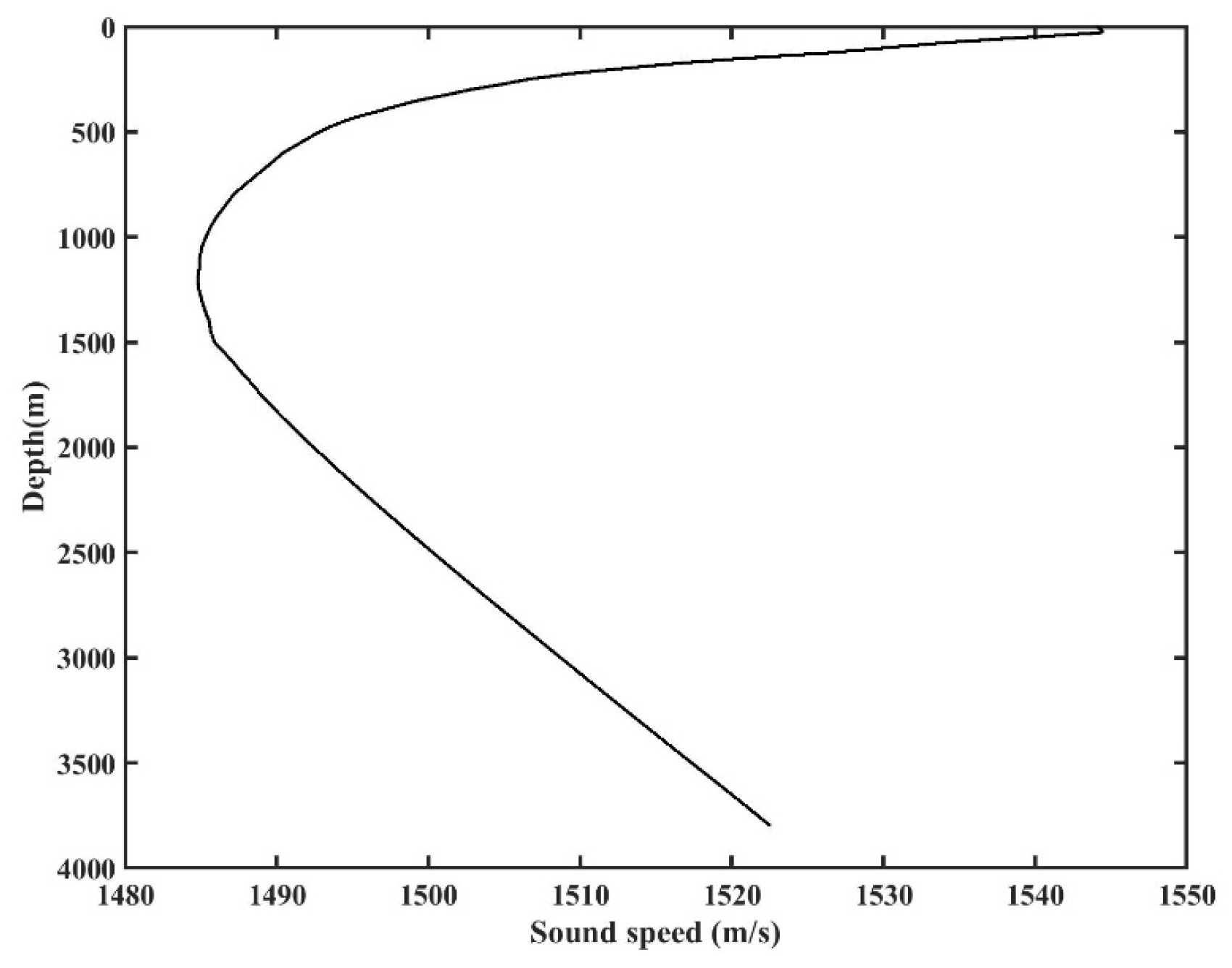
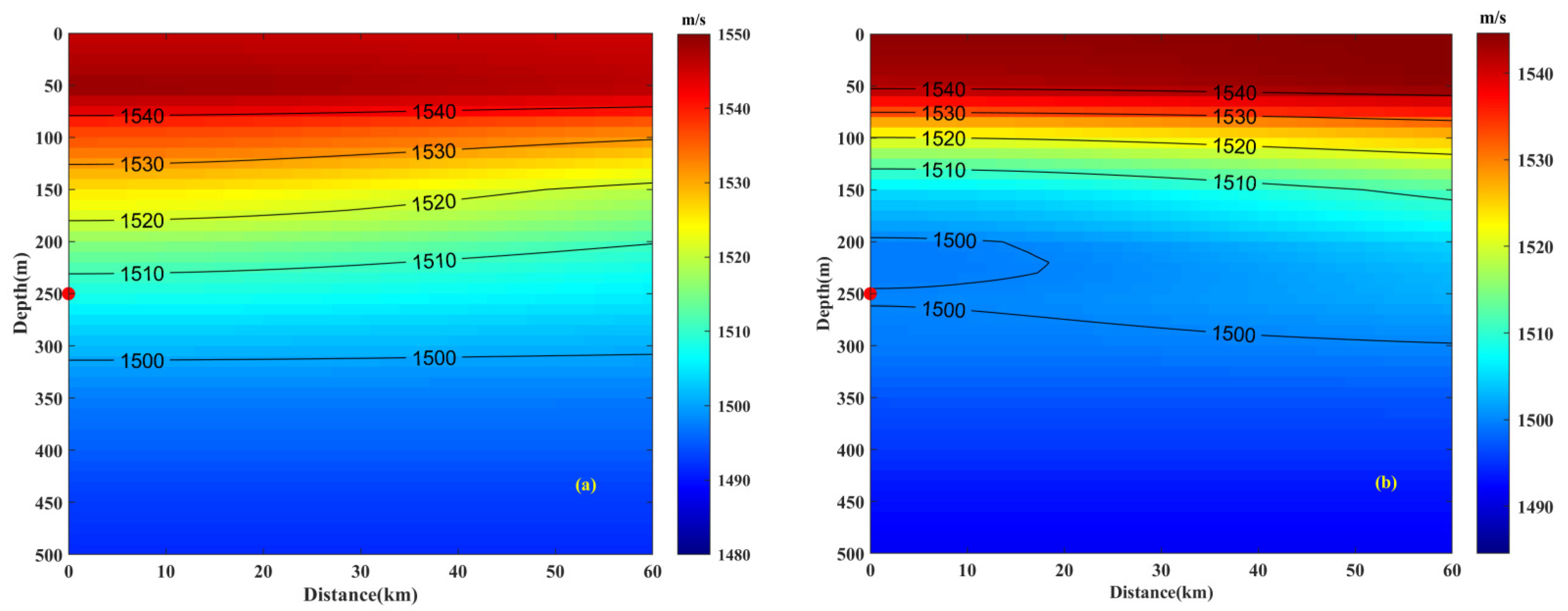
2.1. Sound Propagation Environment

The horizontal scales of oceanic eddies typically vary from tens to hundreds of kilometers, with a lifespan from several weeks to months. Consequently, obtaining synchronized hydrological and acoustic data in the eddy environment during experiments poses a significant challenge. This challenge hinders the fulfillment of research requirements. However, the extensive analysis of satellite remote sensing data reveals several typical structural characteristics of eddies [23], including: (1) an elliptical cross-sectional shape exerting horizontal and vertical influence on seawater and (2) a slow movement speed, appearing quasi-static in comparison to sound propagation speed. Therefore, it is feasible to parameterize the sound speed structure induced by eddies through appropriate models. By integrating these models with sound field calculation methods, it is possible to quantitatively analyze the impact of various eddy parameters on sound propagation characteristics. The Gaussian eddy model [24] is frequently used to reconstruct the sound speed field with the presence of an eddy. Compared to other similar models, the Gaussian eddy model can describe the sound speed field induced by an eddy with fewer parameters, which is suitable for the analysis of eddy effects on the sound field. In the Gaussian eddy model, the expression for sound speed in the r-z cylindrical coordinate plane is given as follows:

$$c(r,z)=c_0(z)+\delta c(r,z),$$

(1)

$$\delta c(r,z)=D_c\times \exp [-{\left(\frac{r-R_{\mathrm{e}}}{D_r}\right)}^2-{\left(\frac{z-Z_{\mathrm{e}}}{D_z}\right)}^2],$$

(2)

where $c_0(z)$ is the sound speed background field, representing the sound speed distribution without an eddy. $\delta c(r,z)$ is the sound speed disturbance caused by an eddy. $D_c$ is the eddy intensity, representing the maximum sound speed disturbance caused by an eddy. This parameter can be negative or positive, corresponding to the environment with a cold or warm eddy, respectively. $R_{\mathrm{e}}$ represents the relative distance between the eddy center and the source. $Z_{\mathrm{e}}$ denotes the depth of the eddy center. $D_r$ is the horizontal influence radius of the eddy. $D_z$ is the vertical influence radius of the eddy.

In numerical analysis, the simulation parameters are chosen based on an experiment conducted in the China Sea. The measured SSP serves as the background field without the influence of an eddy, as illustrated in Figure 1. Figure 2 shows the distribution of sound speed induced by a warm ($D_c$ = 10 m/s) and cold ($D_c$ = −10 m/s) eddy within the depth of 500 m. In these simulations, only the eddy intensity is varied, while all other parameters remain the same. The eddy center ($R_{\mathrm{e}}$) is positioned at a distance of 0 km, with a depth ($Z_{\mathrm{e}}$) of 150 m, a horizontal radius ($D_r$) of 60 km, and a vertical radius ($D_z$) of 100 m, which is a subsurface eddy. The maximum sound speed perturbations in cold and warm eddy environments are 10 m/s and −10 m/s. The simulation configuration is shown in Figure 3, where the seabed remains constant at a depth of 3800 m. Based on sediment sampling results in the China Sea [25], a two-layer seabed model is employed. The model comprises a sediment layer with a thickness of 20 m, a sound speed of 1499 m/s, and a density of 1.36 g/cm³. The homogeneous half-space basement has a sound speed of 1650 m/s and a density of 1.8 g/cm³. The attenuation coefficients for both layers are set to 0.068 $\mathrm{d}\mathrm{B}/\lambda$. The sound source is positioned at the horizontal center of the eddy, with a depth of 250 m and a center frequency of 150 Hz. The signals are generated by the sound field calculation model. To meet the narrowband condition essential for subsequent array gain analysis, only acoustic signals within a frequency range of 145–155 Hz are selected for examination, with a frequency interval of 0.1 Hz and a duration of 10 s.

2.2. Vertical Correlation and Array Gain

The vertical correlation of the sound field is the cross-correlation between acoustic signals received at two points within the ocean waveguide. These points have the same horizontal distance but differ in their receiver depth. The vertical correlation serves to quantify the spatial similarity of the sound field and can be expressed as follows:

$$\rho (△z)=\underset{\tau }{\max }\frac{\mathrm{Re}[{\displaystyle {\int }_{{\omega }_0-△\omega /2}^{{\omega }_0+△\omega /2}{P}_z(\omega )P_{z+△z}^{*}(\omega )e^{\mathrm{j}\omega \tau }\mathrm{d}\omega }]}{\sqrt{{\displaystyle {\int }_{{\omega }_0-△\omega /2}^{{\omega }_0+△\omega /2}{\left|P_z(\omega )\right|}^{2}d\omega }}\sqrt{{\displaystyle {\int }_{{\omega }_0-△\omega /2}^{{\omega }_0+△\omega /2}{\left|P_{z+△z}(\omega )\right|}^2\mathrm{d}\omega }}},$$

(3)

where $\omega$ and $△\omega$ represent the angular frequency and bandwidth of the received signal, respectively. $P$ represents the spectrum of the received signal. * denotes complex conjugation. $\mathrm{Re}$ represents the real part of the calculation result. The threshold for the correlation coefficient is set as $\rho =0.707$, and the vertical correlation radius is defined as the array spacing when the vertical correlation coefficient drops to 0.707.

The array gain is defined as the ratio of the SNR after array processing to the SNR on a single element, and the formula is as follows:

$$\mathrm{A}\mathrm{G}=\frac{\mathrm{S}\mathrm{N}{\mathrm{R}}_{array}}{\mathrm{S}\mathrm{N}{\mathrm{R}}_{\mathrm{elem}}}=10{\log }_{10}\frac{{\left(S/N\right)}_{\mathrm{array}}}{{\left(S/N\right)}_{\mathrm{elem}}},$$

(4)

where $\mathrm{S}\mathrm{N}{\mathrm{R}}_{\mathrm{array}}$ and $\mathrm{S}\mathrm{N}{\mathrm{R}}_{\mathrm{elem}}$ represent the output SNR of an array and a single array element, respectively. $S_{\mathrm{array}}$ and $S_{\mathrm{elem}}$, respectively, denote the output signal power after array processing and the signal power of a single array element, while $N_{\mathrm{array}}$ and $N_{\mathrm{ele}m}$, respectively, represent the output noise power after array processing and the noise power of a single array element. For the sake of maintaining generality, the array gain is obtained by CBF. The conventional beamformer is based on the planewave model whose weighting coefficient can be written as:

$$\mathbf{w}=\exp [-\mathrm{j}{\omega }_0\mathbf{z}\sin \theta /c],$$

(5)

where ${\omega }_0$ represents the center frequency. $\mathbf{z}$ is the distance vector between each element and the first element. $c$ is the sound speed. $\theta$ is the steering angle. The signal vector is defined as:

$$\mathbf{x}(t)={[x_1(t),x_2(t),\cdots ,x_N(t)]}^{\mathrm{T}}.$$

(6)

The cross-correlation matrix of the received signals is:

$${\mathbf{R}}_x=E\left\{\mathbf{x}(t){\mathbf{x}}^H(t)\right\}.$$

(7)

Then the array output and the output power are:

$$y(t,\theta )={\mathbf{w}}^H\left(\theta \right)\mathbf{x}(t),$$

(8)

$$P_{CBF}(\theta )=E\left\{y(t,\theta )y^H(t,\theta )\right\}={\mathbf{w}}^{\mathrm{H}}(\theta ){\mathbf{R}}_x\mathbf{w}(\theta ).$$

(9)

In an ideal scenario, the array gain after beamforming can approach $10{\log }_{10}(N)$, and $N$ is the number of array elements. However, in actual ocean environments, the signal wavefront is distorted due to the influence of the ocean waveguide. As a result, the array gain cannot reach the theoretical limit value.

2.3. Acoustic Modelling Method

Various sound field calculation models have their advantages and disadvantages and can be selected according to the specific requirements. The Bellhop [26] and RAM [27] models can be applied to describe sound propagation in range-dependent environments, which are suitable for acoustic modelling in the mesoscale eddy areas. The RAM model exhibits high precision in calculating the sound field affected by eddies. Furthermore, the result of the ray method is intuitive and clear, which is used to explain the mechanism of sound field characteristics. By integrating these models with simulation environments, the result of sound field calculation models can be obtained and analyzed. The parameter setting of the RAM model is as follows: the vertical resolution is 10 m, and the horizontal resolution is 200 m. The range of grazing angles in the Bellhop model is selected based on actual needs.

3. Results and Discussion

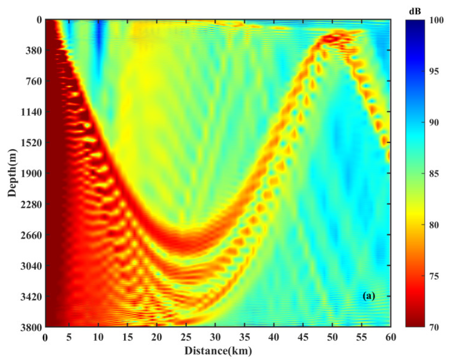
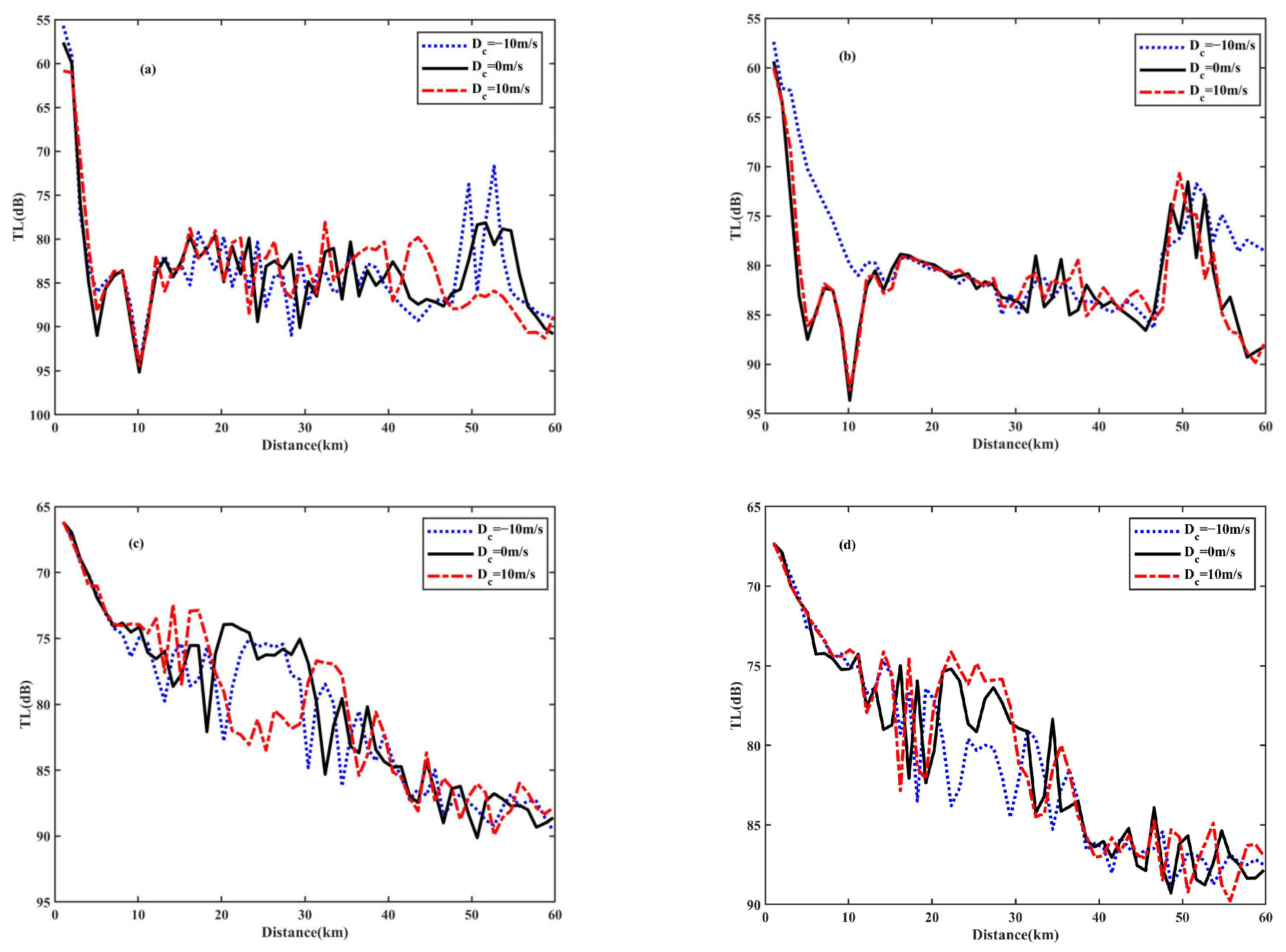
3.1. Transmission Loss Disturbance Analysis

Mesoscale eddies cause the energy redistribution of the sound field, which can be directly reflected by TL. According to the simulation environments shown in Figure 2 and Figure 3, the sound speed distribution induced by the eddy is constructed using the Gaussian eddy model. This distribution is then integrated into the RAM sound field calculation model, which is approximated by the parabolic equation. Subsequently, the eddy-induced differences in TL are numerically analyzed.

Figure 4 shows TL in the range of 60 km with or without an eddy. It can be seen that the environment without an eddy exhibits typical deep-sea sound propagation characteristics, with the propagation distance spanning a complete CZ. Notably, there are striation patterns in the direct sound region, corresponding to four interference beams. By comparing TL in the no-eddy environment with the results under different eddy conditions, it can be observed that: (1) Near the first CZ, the upper turning points are deeper, and the sound energy is more concentrated, influenced by the warm eddy in Figure 4b. Conversely, the cold eddy, as shown in Figure 4c, leads to shallower upper turning points and divergent sound energy. (2) In the ranges of 0~10 km and 50~60 km of Figure 4c, the existence of a cold eddy near the source depth induces the formation of an eddy waveguide with deeper depth and lower sound speed, similar to the classical sound waveguide. While part of the energy propagates in the waveguide, it decays rapidly with distance. (3) Within the range of 20–30 km, the warm eddy (as shown in Figure 4b) deepens the direct sound region, leading to a reduction in the interference beam number and the coverage area. Conversely, in the cold-eddy environment shown in Figure 4c, the corresponding direct sound region becomes shallower, the interference beam number increases, and the coverage area widens.

To accurately analyze the changes in TL affected by the eddy, TLs at four receiver depths (150 m, 250 m, 2700 m, and 3100 m) are presented in Figure 5. The differences of energy distribution in the eddy are quantitatively described through comparison. (1) Within the first CZ, the TL in the warm eddy at a depth of 150 m is approximately 5 dB higher than that in the no-eddy environment, while the TL in the cold eddy is slightly reduced. (2) As shown in Figure 5b, at a receiver depth of 250 m, the cold eddy reduces TL by 10 dB in the ranges of 0–10 km and 50–60 km, while no similar phenomenon is observed under the influence of the warm eddy. (3) In Figure 5c, at a receiver depth of 2700 m, the TL increases by about 6 dB at a distance of 25 km in the warm eddy, whereas the energy changes little in the cold eddy. However, at the same distance, the change in TL at the receiver depth of 3100 m in Figure 5d is different. The TL is slightly reduced in the presence of a warm eddy, while it is increased in the cold eddy.

To explain the differences in TL caused by the eddy in Figure 4 and Figure 5, ray diagrams in the different environments are given in Figure 6, where the black dot represents the sound source located at a depth of 250 m. The red rays indicate the water-refracted paths without bottom bounce. The blue rays indicate the bottom-bounce paths. The cyan rays represent surface-bottom-bounce paths. The black horizontal lines represent different receiver depths, including 150 m, 250 m, 2700 m, and 3100 m. As depicted in Figure 6b, when the receiver depth is 150 m, the presence of a warm eddy increases the sound speed in the upper layer. As a result, the turning points in the CZ deepen, and the refracted paths cannot reach the receiver depth, thus leading to an increase in TL. Conversely, in Figure 6c, the cold eddy reduces the upper sound speed, allowing more refracted paths to reach the receiver depth. As a result, the turning points in the CZ become shallower, leading to a reduction in TL. At a receiver depth of 250 m, there is an eddy waveguide with lower sound speed in Figure 6c. The small-angle launch rays are deflected towards the depth of the cold-eddy waveguide (150 m) within the initial 10 km. This deflection causes a part of the refracted paths propagating in this region. However, the thickness of the waveguide is thin and gradually decreases with distance from the eddy, causing rays to leak from the waveguide after propagating with a certain distance. Furthermore, the TL is small within a distance of 0 to 10 km. The refracted paths affected by the waveguide converge near the first CZ, leading to a uniform ray distribution and an expanded convergence area. As shown in Figure 6b and c, the presence of a warm or cold eddy changes the sound speed at the source, causing the depth of refracted paths to be deeper or shallower, respectively, in the direct sound region. In Figure 6b, at a receiver depth of 2700 m, the refracted paths fail to reach the receiver within the range of 20 to 30 km in the warm eddy, resulting in an increase in TL in this region. At a receiver depth of 3100 m, the deepening of turning points in the warm eddy leads to a concentration of refracted paths, thereby diminishing TL at this depth. Due to different launch angles, the turning-point depths of refracted paths change differently in the cold-eddy environment, as shown in Figure 6c. This variation results in fewer rays within a distance of 20 to 30 km, thus increasing TL at this receiver depth. In summary, the presence of an eddy changes the sound speed at the source location and sound speed horizontal distribution, which ultimately impacts the overall sound field distribution.

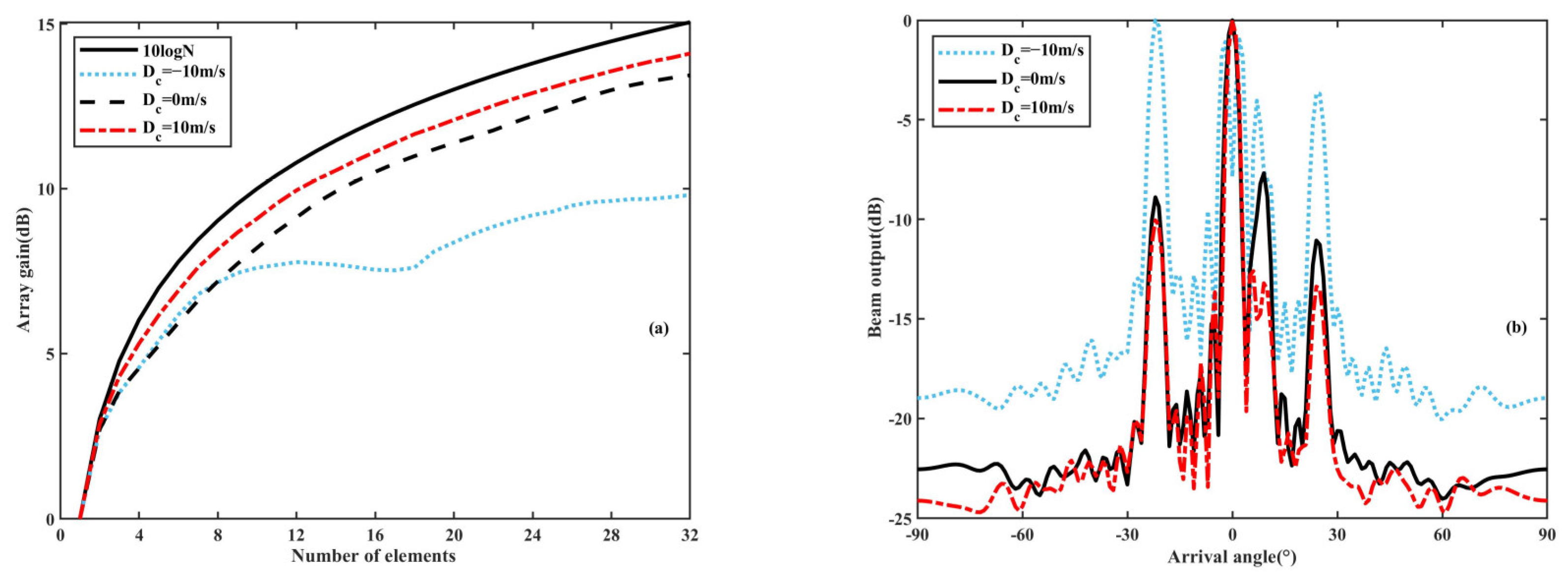
3.2. Effect on Vertical Correlation and Array Gain

The preceding analysis has highlighted the eddy effects on the energy distribution in the sound field. Expanding upon this analysis, the study focuses on the numerical analysis of variations in the vertical correlation of the sound field. It considers different acoustic regions affected by a cold or warm eddy. Moreover, the influence on array gain is studied using the same parameters.

For the purpose of clarity, Figure 7 (same as Figure 4) illustrates the positions of receiver arrays in different eddy environments. In the absence of an eddy, the first CZ is located approximately 50 km away from the source. To analyze the effects of vertical correlation on array gain in the eddy, three sound zones have been selected: the first CZ, the direct sound region and the first shadow zone. These zones are highlighted with black boxes in Figure 7a. In the figure, the black lines represent the positions of the receiver arrays. The environmental parameters used in the numerical calculation are the same as those described in the previous section. The vertical receiver arrays are set at 25 km and 50 km, with the depth ranges of 175~330 m and 3075~3230 m, respectively. The array elements are spaced at intervals of 5 m, ensuring compliance with a half wavelength (150 Hz sound source). Each array comprises 32 elements, labeled consecutively from 1 (uppermost element) to 32 (lowest element). The Gaussian white noise is assumed as the receiving noise of the vertical array, with a SNR of 10 dB for each element. It is evident from Figure 7 that the presence of an eddy affects the received signals of the vertical array and the distribution of sound energy in the specific regions. The vertical correlation in different sound zones and the corresponding changes in the array gain influenced by an eddy are discussed below.

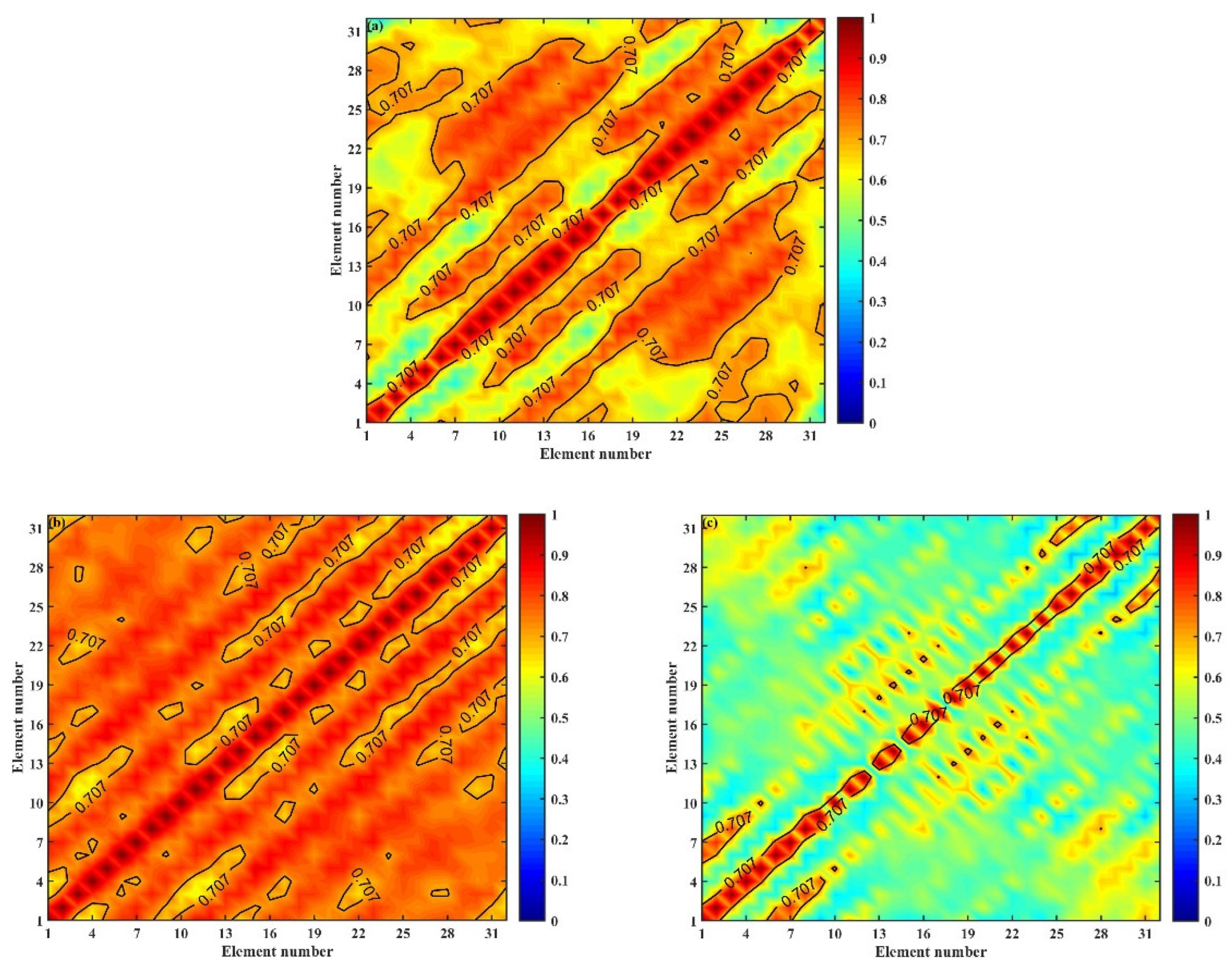
3.2.1. The First Convergence Zone

In the first CZ, a vertical array is located near the sea surface and approximately 50 km away from the sound source. In this region, the sound energy mainly comes from refracted paths. As these paths are turned near the CZ, the sound speed disturbance has a significant impact on the energy distribution. To analyze the vertical correlation of this region in different eddy environments, the Gaussian eddy model is used. Figure 8 shows the vertical correlation coefficient with or without an eddy in the first CZ. By combining Figure 7 and Figure 8, it can be observed that in the absence of an eddy, all the elements are located within the first CZ. In this case, the received signals are mainly contributed by refracted paths, resulting in a high correlation coefficient among each element. However, when a warm eddy exists, the vertical correlation coefficients between the shallower elements decrease rapidly. Conversely, in the case of a cold eddy, the correlation coefficients in the region decrease slightly overall, but individual array elements exhibit a significant decrease. This phenomenon is primarily attributed to the deepening of turning points in the CZ, which is induced by the warm eddy. As a result, the shallow receiver elements are outside the CZ (Figure 7b), causing the arrivals to be complex and a decline in vertical correlation. On the other hand, the cold eddy makes the CZ shallower and the energy distribution more divergent (Figure 7c). Consequently, the vertical correlation is affected, which is consistent with the change in TL in Figure 5a.

To further explain the influence of eddies on vertical correlation, Figure 9 shows the corresponding eigenrays and time-arrival structures in the first CZ for the environments with or without an eddy. The receiver depth is 250 m, corresponding to the central depth of an array. The black dots respect the source and receiver. Different colors are used to distinguish the interaction frequency of rays with the bottom or sea surface, and the meanings are the same as those in Figure 6. The line with circle respects the amplitude of the different path. As can be seen from Figure 9, there are differences in eigenrays and time-arrival structures across different eddy environments. When there is no eddy, the multipath structure at the receiver is the simplest, and the main contribution to the sound field is a cluster of refracted paths corresponding to a small grazing angle. However, the multipath structure induced by an eddy becomes relatively complex, where the primary contribution comprises two clusters of rays with comparable amplitude. Moreover, the eddy affects the turning-point depths of the eigenrays, resulting in a smaller time difference in the warm eddy and a larger time difference in the cold eddy. This difference in the multipath structure is mainly caused by the horizontally non-uniform distribution of sound speed. Consequently, two clusters of rays arrive with comparable absolute amplitudes, resulting in a generally smaller vertical correlation in eddy environments compared to no-eddy environments.

The array gain and beam output in the first CZ for environments with or without an eddy are shown in Figure 10, with the theoretical limit of the array gain $10{\log }_{10}(N)$. It can be seen that the arrival angle is near 0°, corresponding to the refracted paths turned in this region. With the increase in the number of elements, the array gain in this region increases first and then decreases. Additionally, the array gain in the absence of an eddy exceeds that in eddy environments. Specifically, when the number of elements is small (n < 5), the array gain in a warm eddy is smaller than that in other environments. However, as the element number increases, the array gain increases rapidly in the warm eddy. Combined with Figure 7 and Figure 8, it is evident that for small element numbers (n < 5), the array elements are located outside the first CZ, resulting in a decrease in vertical correlation and array gain. Nonetheless, with an increase in array elements, some array elements are located in the first CZ, leading to a continuous improvement in vertical correlation and array gain in the warm eddy. Similarly, there is a corresponding relationship between vertical correlation and array gain in the cold eddy. When the number of array elements exceeds a certain threshold, some elements of the vertical array are outside the first CZ, leading to a decrease in vertical correlation and array gain. Ultimately, when n = 32, the differences in beam output and array gain among various environments become small.

In various eddy environments, the correlation distribution among array elements in the first CZ differs. Nonetheless, the element near the center of the vertical array always maintains a high correlation coefficient (see Figure 8). To further analyze the impact of vertical correlation on array gain, the beamforming method starts from regions of high correlation to those of low correlation. The array gain results of this approach across different eddy environments are obtained and illustrated in Figure 11. Notably, the analysis reveals that as elements are numbered outward from the middle in the receiver array, the correlation generally remains high, and the curve of the array gain with respect to the element number is relatively smooth. This trend differs from the rapid increase in array gain observed after n = 5 in the warm eddy, as depicted in Figure 10. With an increase in the element number to 15 (corresponding to the high correlation region), the array gain tends to saturate in both cold and warm-eddy environments, whereas saturation occurs around n = 20 in the no-eddy environment. It is crucial to emphasize that, for the entire receiver array with n = 32, the beamforming sequence does not alter the overall array gain results across different eddy environments. However, when the beamforming method starts from regions of high correlation, it significantly improves the corresponding array gain, especially with a smaller number of array elements.

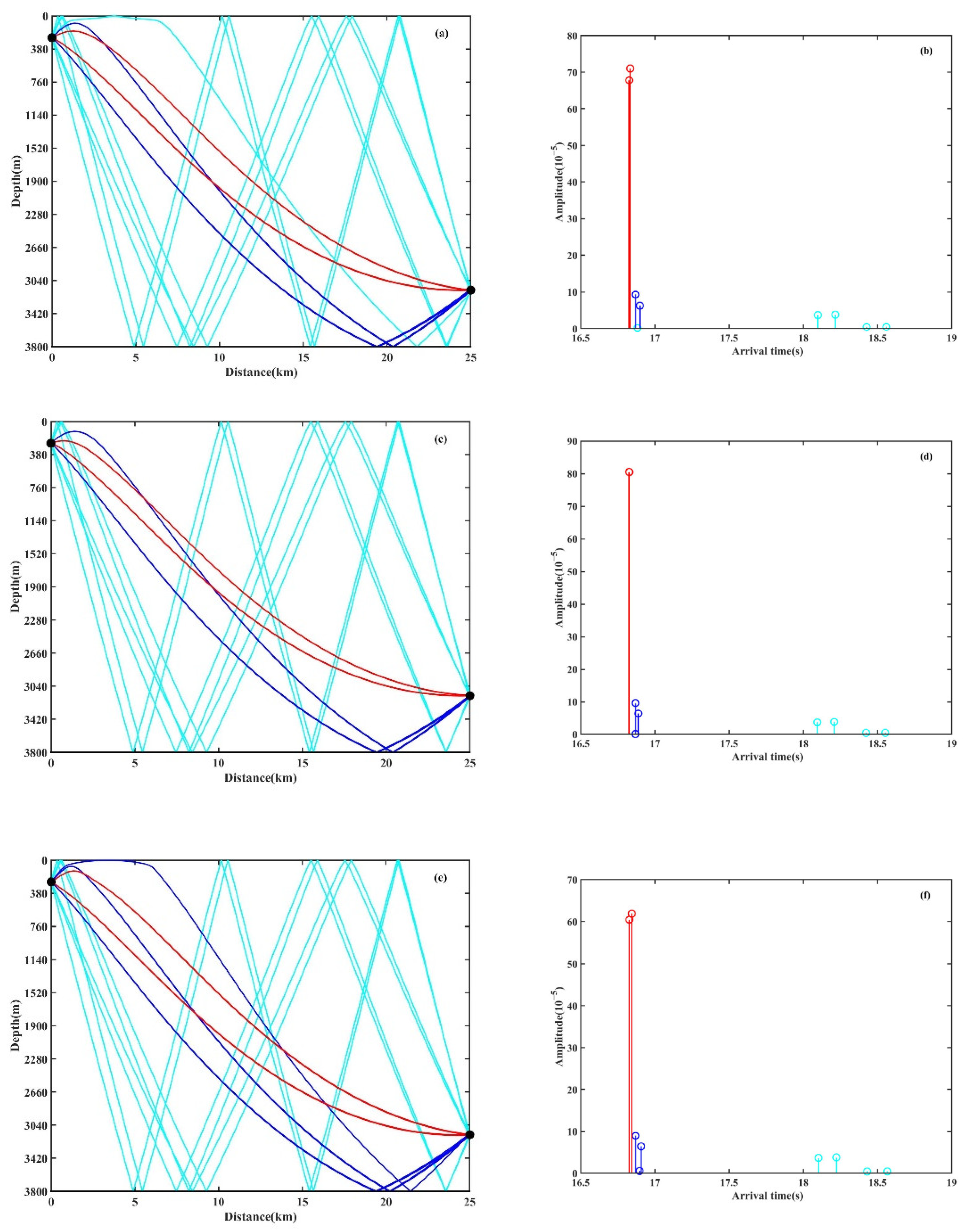
3.2.2. The Direct Sound Region

The vertical array is placed at a large depth of 25 km from the sound source in the direct sound region. The main rays are refracted without bottom bounce in this area, resulting in a large amount of sound energy. The vertical correlation with or without an eddy in the direct sound region is shown in Figure 12. As observed in Figure 7 and Figure 12, when there is no eddy ($D_c$ = 0 m/s), each element is located at the second interference beam in the direct sound region (Figure 7a), leading to a good vertical correlation, while the correlation coefficient diminishes as the elements move away from the center. In the presence of a warm eddy ($D_c$ = 10 m/s), the entire vertical correlation is high. This can be attributed to the warm eddy that deepens the turning points in the direct sound region, thereby placing the entire vertical array within the first interference beam (Figure 7b). On the other hand, the existence of a cold eddy ($D_c$ = −10 m/s) results in a rapid decrease in vertical correlation. This decline occurs due to the presence of a cold eddy, as illustrated in Figure 7c, causing the turning points to be shallow. Consequently, the elements are located outside the interference beam, consistent with the change in TL in Figure 5d.

To explain the impact of eddies on vertical correlation in the direct sound region, Figure 13 illustrates the corresponding eigenrays and time-arrival structures in the direct sound region for the environments with or without an eddy. The black dots respect the source and receiver. The line with circle respects the amplitude of the different path. The receiver depth, set at 3150 m, corresponds to the central depth of an array. It can be observed that the types of eigenrays and the time-arrival structures are similar across different eddy environments. When there is no eddy, the main contributions to the sound energy at the receiver depth are two refracted rays with similar paths, amplitudes, and arrival times. However, due to the different launch angles of refracted rays, the lower turning-point depths of rays are affected differently by eddies, leading to variations in the corresponding multipath arrival structure. In the case of a warm eddy, the down-turning depths of rays are deepened, causing the two direct paths to arrive almost simultaneously. This minimization of the time difference between the two paths enhances the vertical correlation. Conversely, in the cold eddy, the down-turning depths of rays become shallower, resulting in an increased distance between two direct paths and a larger time difference. Consequently, the vertical correlation in the cold eddy is lower compared to the other two environments.

The array gain and beam output in the direct sound region for the environments with or without an eddy are shown in Figure 14. In warm-eddy and no-eddy environments, it is evident that the direct paths mainly contribute to the sound field, with arrival angles of around 0°. However, in a cold eddy, there are multiple arrival angles present. The array gain in the warm eddy is larger than in the other environments. As the element number increases, the array gain in the warm eddy increases continuously, but the array gain tends to saturate in the presence of a cold eddy, resulting in a significant difference between the two environments. The disparity arises due to the distinct effects of the eddies on the sound propagation. As shown in Figure 7b, the warm eddy makes the vertical array locate in the first interference beam, thereby concentrating the arrival angles of the main rays and enhancing the correlation coefficients among the array elements. Conversely, as depicted in Figure 7c, the cold eddy makes the turning points of direct paths shallow, causing the vertical array to lie outside the interference beam. Consequently, signals coming from multiple directions and the interference of different paths lead to dispersed energy distribution, decreased vertical correlation, and reduced array gain.

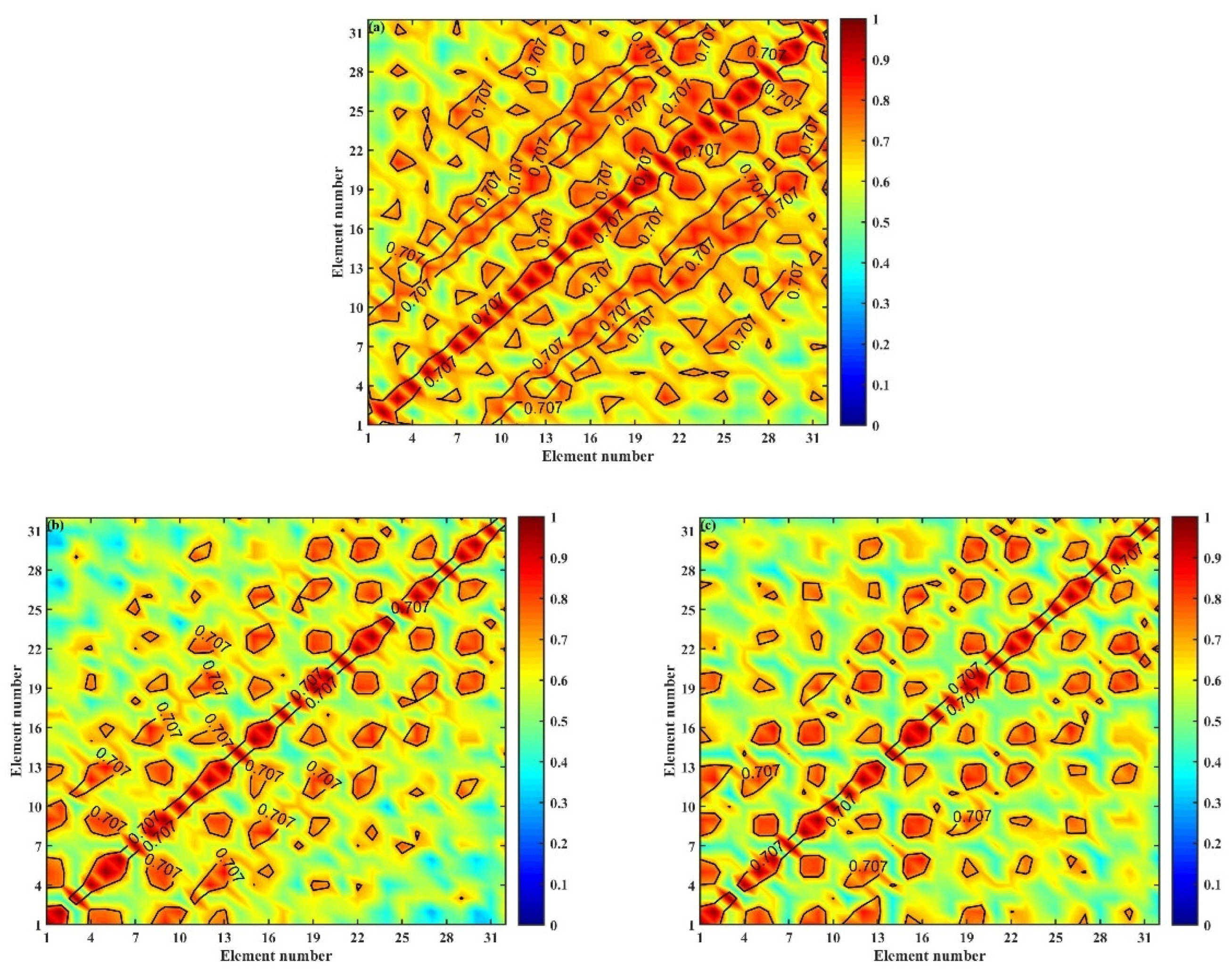
3.2.3. The First Shadow Zone

The vertical array is placed in the first shadow zone near the sea surface, approximately 25 km away from sound source. In this region, there is no direct path, and only the bottom-bounce paths are received. Figure 15 shows the vertical correlation coefficient in the first shadow zone under the environments with or without an eddy. It can be observed from Figure 7 and Figure 15 that the vertical correlation coefficient in the first shadow zone remains relatively stable regardless of element positions. This observation suggests that the existence of an eddy has little impact on the vertical correlation in this region. The main contribution to the sound field in the first shadow zone are the bottom-bounce paths. As a result of these complex multipath interference patterns, the received signal pulse of each element is relatively complex. Therefore, the vertical correlation in this region is generally low. Moreover, this area is characterized by rays with large launch angles, which have more interaction with the bottom and are less affected by sound speed disturbance. Therefore, the received signals have little impact from the eddy, and changes in the vertical correlation are not obvious. In practice, the SNR of received signals in the shadow zone is lower compared to the direct sound region and the first CZ. Hence, the corresponding vertical correlation in the shadow zone will further decline due to the lower SNR.

To explain the impact of eddies on vertical correlation in the first shadow zone, Figure 16 illustrates the corresponding eigenrays and time-arrival structures in the first shadow zone for the environments with or without an eddy. The black dots respect the source and receiver. The receiver depth of 250 m corresponds to the central depth of an array. Notably, the types of eigenrays and the time-arrival structures are almost unchanged across different eddy environments. The received signals, corresponding to large launch angles, exhibit little variations in amplitude and arrival time across different eddy-induced environments. Therefore, this phenomenon results in a small difference in vertical correlation attributed to the presence of an eddy.

The array gain and beam output in the first shadow zone for the environments with or without an eddy are shown in Figure 17. It can be seen from the figure that the main directions of arrivals are concentrated at angles of 20° and −20°, corresponding to surface paths and bottom-surface bounce paths, respectively. When the receiver array is located in the first shadow zone, a significant reduction in the array gain is observed compared to that in the direct sound region due to the weakening of correlation. With the increase in elements, the array gain keeps increasing. However, among different eddy environments, the array gain remains relatively similar, with a difference of only about 1 dB, which is consistent with the change in the vertical correlation coefficient in Figure 15. In addition, in the first shadow zone, it is evident that the energy of main arrivals is affected by the eddy. Specifically, the energy is observed to be more concentrated and distinct in the eddy environment. Moreover, the corresponding array gain is slightly higher than that in the no-eddy environment.

4. Conclusions

The present study investigates the characteristics of the sound field with eddy disturbance by employing a Gaussian eddy model. This model constructs the distribution of sound speed, which is subsequently used as the parameter input for the sound field calculation model. Specifically, the propagation properties in the environment with or without an eddy are compared. Additionally, the vertical correlation differences of sound fields in typical regions with an eddy and their effects on the array gain using CBF are studied.

The presence of an eddy introduces perturbations in the sound speed field along the sound propagation path and redistributes the energy in the ocean. When the sound source is near the center of an eddy, the cold eddy promotes the formation of a cold-eddy waveguide. As a result, a part of the energy propagates within this waveguide, leading to the emergence of a high-energy region and the reduction in TL by 10 dB. Conversely, the warm eddy deepens the turning points in the first CZ, resulting in an increase of approximately 5 dB in TL compared to the no-eddy environment. Moreover, the presence of an eddy can change the coverage of the direct sound region, leading to a redistribution of sound field energy within that region. However, the eddy has little influence on TL in the first shadow zone.

The environment between the source and the receiver array can be disturbed by the presence of eddies, leading to changes in the amplitude and phase of received signals at the array elements. Moreover, these eddies alter the vertical correlation of the sound field, consequently impacting the array gain. This paper focuses on the relationship between vertical correlation and array gain with varying eddy intensities.

It is found that the vertical correlation is relatively high in the first CZ, while the vertical correlation in the direct sound region is significantly affected by the eddy, and the influence of the eddy on the first shadow zone is minimal. Moreover, there is a positive correlation between array gain and vertical correlation. Specifically, when the sound field correlation is good, the array gain increases with the number of array elements. The research results provide important guidance for the performance analysis and practical application of vertical arrays in mesoscale eddy environments.

References

1. Abraham, D.A. Underwater Acoustic Signal Processing: Modeling, Detection, and Estimation; Springer: Cham, Switzerland, 2019. [Google Scholar]
2. Sun, D.J.; Zheng, C.E.; Zhang, J.C.; Han, Y.F.; Cui, H.Y. Development and prospect for underwater acoustic positioning and navigation technology. Chin. Acad. Sci. 2019, 34, 331–338. [Google Scholar] [CrossRef]
3. Colosi, J.A.; Chandrayadula, T.K.; Voronovich, A.G.; Ostashev, V.E. Coupled mode transport theory for sound transmission through an ocean with random sound speed perturbations: Coherence in deep water environments. J. Acoust. Soc. Am. 2013, 134, 3119–3133. [Google Scholar] [CrossRef] [PubMed]
4. Dong, F.C.; Hu, Z.G.; Li, Z.L. Effects of uneven bottom on vertical correlation of sound field in the deep water area of the South China Sea. Chin. Acta Acust. 2020, 45, 785–800. [Google Scholar] [CrossRef]
5. Hu, Z.G.; Li, Z.L.; Zhang, R.H.; Ren, Y.; Li, J. The effects of the uneven bottom on horizontal longitudinal correlation of acoustic field in the deep water. Chin. Acta Acust. 2016, 41, 758–767. [Google Scholar] [CrossRef]
6. Cox, H. Line array performance when the signal coherence is spatially dependent. J. Acoust. Soc. Am. 1973, 54, 1743–1746. [Google Scholar] [CrossRef]
7. Carey, W.; Reese, J.; Bucker, H. Environmental acoustic influences on array beam response. J. Acoust. Soc. Am. 1998, 104, 133–140. [Google Scholar] [CrossRef]
8. Morgan, D.R.; Smith, T.M. Coherence effects on the detection performance of quadratic array processors, with applications to large-array matched-field beamforming. J. Acoust. Soc. Am. 1990, 87, 737–747. [Google Scholar] [CrossRef]
9. Zavol’skii, N.; Malekhanov, A.; Raevskii, M.; Smirnov, A. Effects of wind waves on horizontal array performance in shallow-water conditions. Acoust. Phys. 2017, 63, 542–552. [Google Scholar] [CrossRef]
10. Xie, L.; Sun, C.; Liu, X.H.; Jiang, G.Y. Array gain of conventional beamformer affected by structure of acoustic field in continental slope area. Acta Phys. Sin. 2016, 65, 171–181. [Google Scholar] [CrossRef]
11. Urick, R. Measurements of the vertical coherence of the sound from a near-surface source in the sea and the effect on the gain of an additive vertical array. J. Acoust. Soc. Am. 1973, 54, 115–120. [Google Scholar] [CrossRef]
12. Dong, F.; Li, Z.; Hu, Z.; Wu, S. The Effects of Vertical Correlation Characteristics on Vertical Array Gain Performance in Deep Water. IEEE J. Ocean. Eng. 2022, 47, 751–766. [Google Scholar] [CrossRef]
13. Smith, G.C.; Fortin, A.-S. Verification of eddy properties in operational oceanographic analysis systems. Ocean. Model. 2022, 172, 101982. [Google Scholar] [CrossRef]
14. Chen, W.; Zhang, Y.C.; Liu, Y.Y.; Ma, L.N.; Wang, H.D.; Ren, K.J.; Chen, S.Y. Parametric Model for Eddies-Induced Sound Speed Anomaly in Five Active Mesoscale Eddy Regions. J. Geophys. Res. Oceans. 2022, 127, 018408. [Google Scholar] [CrossRef]
15. Evans, D.G.; Frajka Williams, E.; Naveira Garabato, A.C.; Polzin, K.L.; Forryan, A. Mesoscale eddy dissipation by a ‘Zoo’ of submesoscale processes at a western boundary. J. Geophys. Res. Oceans 2020, 125, 016246. [Google Scholar] [CrossRef]
16. Liu, J.Q.; Piao, S.C.; Gong, L.J.; Zhang, M.H.; Guo, Y.C.; Zhang, S.Z. The Effect of Mesoscale Eddy on the Characteristic of Sound Propagation. J. Mar. Sci. Eng. 2021, 9, 787. [Google Scholar] [CrossRef]
17. Heaney, K.D.; Campbell, R.L. Three-dimensional parabolic equation modeling of mesoscale eddy deflection. J. Acoust. Soc. Am 2016, 139, 918–926. [Google Scholar] [CrossRef]
18. Xiao, Y.; Li, Z.; Li, J.; Liu, J.; Sabra, K.G. Influence of warm eddies on sound propagation in the Gulf of Mexico. Chin. Phys. B 2019, 28, 054301. [Google Scholar] [CrossRef]
19. Gao, F.; Xu, F.H.; Li, Z.L. The Effects of Mesoscale Eddies on Spatial Coherence of Middle Range Sound Field in Deep Water. Chin. Phys. B 2022, 11, 114302. [Google Scholar] [CrossRef]
20. Hassantabar Bozroudi, S.H.; Ciani, D.; Mohammad Mahdizadeh, M.; Akbarinasab, M.; Aguiar, A.C.B.; Peliz, A.; Chapron, B.; Fablet, R.; Carton, X. Effect of Subsurface Mediterranean Water Eddies on Sound Propagation Using ROMS Output and the Bellhop Model. Water 2021, 13, 3617. [Google Scholar] [CrossRef]
21. Khan, S.; Song, Y.; Huang, J.; Piao, S. Analysis of Underwater Acoustic Propagation under the Influence of Mesoscale Ocean Vortices. J. Mar. Sci. Eng. 2021, 9, 799. [Google Scholar] [CrossRef]
22. Liu, Y.; Xu, J.; Jin, K.; Feng, R.; Xu, L.; Chen, L.; Chen, D.; Qiao, J. A FEM Flow Impact Acoustic Model Applied to Rapid Computation of Ocean-Acoustic Remote Sensing in Mesoscale Eddy Seas. Remote Sens. 2024, 16, 326. [Google Scholar] [CrossRef]
23. Della Penna, A.; Gaube, P. Mesoscale Eddies Structure Mesopelagic Communities. Front. Mar. Sci. 2020, 7, 454. [Google Scholar] [CrossRef]
24. Shang, E.C. Ocean acoustic tomography based on adiabatic mode theory. J. Acoust. Soc. Am. 1989, 85, 1531–1537. [Google Scholar] [CrossRef]
25. Zhang, P.; Li, Z.L.; Wu, L.X.; Zhang, R.H.; Qin, J.X. Characteristics of convergence zone formed by bottom reflection in deep water. Acta Phys. Sin. 2019, 68, 174–185. [Google Scholar] [CrossRef]
26. Porter, M.B.; Bucker, H.P. Gaussian beam tracing for computing ocean acoustic fields. J. Acoust. Soc. Am. 1987, 82, 1349–1359. [Google Scholar] [CrossRef]
27. Collins, M.D. A split-step Padé solution for the parabolic equation method. J. Acoust. Soc. Am. 1993, 93, 1736–1742. [Google Scholar] [CrossRef]
Figure 1. Background sound speed measured during an experiment conducted in the China Sea.
Remotesensing 16 01862 g001
Figure 2. Distribution of sound speed for the environments with an eddy within the depth of 500 m; (a) a warm eddy ( D c  = 10 m/s), (b) a cold eddy ( D c  = −10 m/s). The red dot respects the sound source.
Remotesensing 16 01862 g002
Figure 3. Simulation configuration.
Remotesensing 16 01862 g003
Figure 4. TL for the environments with or without an eddy; (a) no eddy ( D c  = 0 m/s), (b) a warm eddy ( D c  = 10 m/s), and (c) a cold eddy ( D c  = −10 m/s). The areas enclosed by black dotted boxes are the main areas for discussion.
Remotesensing 16 01862 g004aRemotesensing 16 01862 g004b
Figure 5. Comparison of transmission loss for the environments with or without an eddy at different receiver depths. (a) 150 m, (b) 250 m, (c) 2700 m, and (d) 3100 m.
Remotesensing 16 01862 g005
Figure 6. Ray traces for the environments with or without an eddy; (a) no eddy ( D c  = 0 m/s), (b) a warm eddy ( D c  = 10 m/s), and (c) a cold eddy ( D c  = −10 m/s).
Remotesensing 16 01862 g006aRemotesensing 16 01862 g006b
Figure 7. Positions of receiver arrays for the environments with or without an eddy; (a) no eddy ( D c  = 0 m/s), (b) a warm eddy ( D c  = 10 m/s), and (c) a cold eddy ( D c  = −10 m/s).
Remotesensing 16 01862 g007aRemotesensing 16 01862 g007b
Figure 8. Vertical correlation coefficient in the first convergence zone for the environments with or without an eddy; (a) no eddy ( D c  = 0 m/s), (b) a warm eddy ( D c  = 10 m/s), and (c) a cold eddy ( D c  = −10 m/s). The values on the diagonal are equal to 1.
Remotesensing 16 01862 g008aRemotesensing 16 01862 g008b
Figure 9. Eigenrays and time arrivals at the depth of 250 m in the first convergence zone for the environments with or without an eddy; (a) the eigenrays without an eddy ( D c  = 0 m/s), (b) the time arrivals without an eddy ( D c  = 0 m/s), (c) the eigenrays with a warm eddy ( D c  = 10 m/s), (d) the time arrivals with a warm eddy ( D c  = 10 m/s), (e) the eigenrays with a cold eddy ( D c  = −10 m/s), and (f) the time arrivals with a cold eddy ( D c  = −10 m/s). The red and blue colors indicate the water-refracted path without bottom bounce and the bottom-bounce path, respectively.
Remotesensing 16 01862 g009aRemotesensing 16 01862 g009b
Figure 10. Array gain and beam output in the first convergence zone for the environments with or without an eddy; (a) array gain with the number of array elements and (b) beam output.
Remotesensing 16 01862 g010
Figure 11. Array gain in the first convergence zone for the environments with or without an eddy (the smaller element numbers, the closer to the array center).
Remotesensing 16 01862 g011
Figure 12. Vertical correlation coefficient in the direct sound region for the environments with or without an eddy; (a) no eddy ( D c  = 0 m/s), (b) a warm eddy ( D c  = 10 m/s), and (c) a cold eddy ( D c  = −10 m/s). The values on the diagonal are equal to 1.
Remotesensing 16 01862 g012
Figure 13. Eigenrays and time arrivals at the depth of 3150 m in the direct sound region for the environments with or without an eddy; (a) the eigenrays without an eddy ( D c  = 0 m/s), (b) the time arrivals without an eddy ( D c  = 0 m/s), (c) the eigenrays with a warm eddy ( D c  = 10 m/s), (d) the time arrivals with a warm eddy ( D c  = 10 m/s), (e) the eigenrays with a cold eddy ( D c  = −10 m/s), and (f) the time arrivals with a cold eddy ( D c  = −10 m/s). The red, blue and cyan colors indicate the water-refracted path without bottom bounce, the bottom-bounce path, and surface-bottom-bounce path, respectively.
Remotesensing 16 01862 g013
Figure 14. Array gain and beam output in the direct sound region for the environments with or without an eddy; (a) array gain with the number of array elements and (b) beam output.
Remotesensing 16 01862 g014
Figure 15. Vertical correlation coefficient in the shadow zone for the environments with or without an eddy; (a) no eddy ( D c  = 0 m/s), (b) a warm eddy ( D c  = 10 m/s), and (c) a cold eddy ( D c  = −10 m/s). The values on the diagonal are equal to 1.
Remotesensing 16 01862 g015
Figure 16. Eigenrays and time arrivals at the depth of 250 m in the first shadow zone for the environments with or without an eddy; (a) the eigenrays without an eddy ( D c  = 0 m/s), (b) the time arrivals without an eddy ( D c  = 0 m/s), (c) the eigenrays with a warm eddy ( D c  = 10 m/s), (d) the time arrivals with a warm eddy ( D c  = 10 m/s), (e) the eigenrays with a cold eddy ( D c  = −10 m/s), and (f) the time arrivals with a cold eddy ( D c  = −10 m/s). The blue and cyan colors indicate the bottom-bounce path and surface-bottom-bounce path, re-spectively.
Remotesensing 16 01862 g016aRemotesensing 16 01862 g016b
Figure 17. Array gain and beam output in the first shadow zone for the environments with or without an eddy; (a) array gain with the number of array elements and (b) beam output.
Remotesensing 16 01862 g017
Disclaimer/Publisher’s Note: The statements, opinions and data contained in all publications are solely those of the individual author(s) and contributor(s) and not of MDPI and/or the editor(s). MDPI and/or the editor(s) disclaim responsibility for any injury to people or property resulting from any ideas, methods, instructions or products referred to in the content.