A Machine-Learning-Based Framework for Retrieving Water Quality Parameters in Urban Rivers Using UAV Hyperspectral Images

Abstract

Efficient monitoring of water quality parameters (WQPs) is crucial for environmental health. Drone hyperspectral images have offered the potential for the flexible and accurate retrieval of WQPs. However, a machine learning (ML)-based multi-process strategy for WQP inversion has yet to be established. Taking a typical urban river in Guangzhou city, China, as the study area, this paper proposes a machine learning-based strategy combining spectral preprocessing and ML regression models with ground truth WQP data. Fractional order derivation (FOD) and discrete wavelet transform (DWT) methods were used to explore potential spectral information. Then, multiple methods were applied to select sensitive features. Three modeling strategies were constructed for retrieving four WQPs, including the Secchi depth (SD), turbidity (TUB), total phosphorus (TP), and permanganate index (COD_Mn). The highest R²s were 0.68, 0.90, 0.70, and 0.96, respectively, with corresponding RMSEs of 13.73 cm, 6.50 NTU, 0.06 mg/L, and 0.20 mg/L. Decision tree regression (DTR) was found to have the potential with the best performance for the first three WQPs, and eXtreme Gradient Boosting Regression (XGBR) for the COD_Mn. Moreover, tailored feature selection methods emphasize the importance of fitting processing strategies for specific parameters. This study provides an effective framework for WQP inversion that combines spectra mining and extraction based on drone hyperspectral images, supporting water quality monitoring and management in urban rivers.

1. Introduction

A healthy water environment is essential for urban sustainable development. However, with rapid urbanization and population growth in recent decades, industrial wastewater and domestic sewage discharge into urban rivers has severely degraded water quality, negatively impacting human health and aquatic ecosystems. Water pollution has become a global public health concern [1], necessitating timely and effective water quality monitoring as a prerequisite for urban ecological protection and management. Traditional monitoring methods based on manual sampling are costly and labor-intensive. In recent years, satellite images, such as MODIS, Landsat, and Sentinel, have emerged as a crucial means for detecting inland water quality parameters (WQPs) [2,3] due to their advantages of having a wide monitoring range [4], high efficiency, and low cost [5]. However, for non-optically active parameters such as the total phosphorus (TP) and permanganate index (COD_Mn), the spectral characteristics within the visible–shortwave infrared range are imprecise, resulting in a limited accuracy from traditional satellite sensors for WQP inversion [6]. Moreover, in densely urbanized cities, urban rivers commonly exhibit widths ranging between 10 and 30 m [7]. These rivers present intricate spectral attributes and are highly susceptible to alterations in water quality due to human activities. However, satellite images usually capture data with relatively coarse spatial and spectral resolutions [8]. Therefore, the real-time and acceptable quantitative inversion of WQPs in small-to-medium-sized urban rivers requires support from images with higher spatial and spectral resolutions.

The development of unmanned aerial vehicle (UAV) systems and airborne sensors has presented new opportunities for the remote sensing identification of WQPs in urban rivers [9,10]. UAV systems, due to their flexibility, real-time capabilities, and efficiency, have overcome limitations associated with satellite images, namely the restricted revisit time and information losses in cloudy and rainy weather [11], providing higher spatial resolution images [12] and filling the gaps between ground-based and satellite monitoring. Compared with multispectral images, hyperspectral imagers can rapidly acquire tens or hundreds of high-resolution, narrow-band spectral images [13], offering abundant spectral information [14] and opportunities for the inversion of non-optically active WQPs such as the chemical oxygen demand [6]. UAV hyperspectral images have already found extensive applications in agriculture [15,16,17], with various strategies involving spectral preprocessing, feature selection, and regression modeling [18]. However, the utilization of UAV-borne hyperspectral images for water quality inversion has just witnessed gradual advancement in recent years [19,20]. Limited water quality samples, synchronized UAV images, and the complexity of spectral features in water bodies have emerged as obstacles [14,21,22].

Hyperspectral images present a significant data volume, resulting in information redundancy and computational complexity [15]. Consequently, adopting efficient and dependable methods to uncover and extract valuable spectral information becomes imperative [23]. Spectral preprocessing plays a vital role in reducing noise and enhancing spectral characteristics [16]. Common methods encompass Savitzky–Golay (SG) smoothing, first and second derivatives, singular value decomposition, etc. Fractional order derivation (FOD) has been adopted to explore more subtle spectral details beyond integer orders [16,23]. Combining FOD and discrete wavelet transform (DWT) methods to denoise hyperspectral images has demonstrated improvements, as the R² for the total nitrogen (TN) concentration based on preprocessed reflectance notably surpassed that obtained using original reflectance (OR) data [23].

Feature selection methods curtail the dimensionality of input data by choosing minimally redundant and collinear bands from the full spectra [24]. These methods eliminate noise and unimportant information, thus enhancing model accuracy and robustness [17,25], while also reducing computation time [26]. However, feature selection methods have been seldom used in water quality retrieval using airborne hyperspectral images. Additionally, few studies have compared the effects of diverse feature selection techniques. Some studies [16] selected input variables with the recursive feature elimination (RFE) algorithm, revealing a higher estimation accuracy. Overall, the spectral preprocessing that integrates both spectral transformation and feature selection remains relatively restricted in water quality inversion.

The construction of inversion models is a pivotal step in establishing the mapping relationship between spectral features and WQPs. Nevertheless, empirical methods are confined by samples [27,28], and optical estimation approaches are constrained to the inversion of optical-sensitive parameters. It is challenging to perform inversions for non-optically active parameters like TP [6]. In contrast, in complex inland aquatic environments, machine learning (ML) techniques can accurately discern linear and nonlinear relationships [29] between image spectra and ground data [30]. They have been proven to be effective in identifying various WQPs, particularly non-optically active ones [6,31]. Classic ML algorithms like Random Forest (RF) and eXtreme Gradient Boosting (XGBoost) have been frequently applied [32,33]. In addition to individual ML models [34], some studies have integrated multiple ML algorithms [22] to capitalize on their strengths and achieve higher precision [8]. Moreover, some deep learning (DL) frameworks quantified multiple WQPs and achieved high accuracies [31,35,36]. But the process is comparatively intricate, and the scarcity of sampling data challenges the applicability of these methods in other regions. In summary, the current studies on water quality inversion mainly focus on spectra exploration and the improvement of regression models. However, a comprehensive multi-process combination strategy for water quality inversion based on drone hyperspectral images has yet to be established.

Based on UAV-borne hyperspectral images, this paper aims to: (1) validate the effectiveness of FOD, DWT, and feature selection in the inversion of WQPs; (2) compare the regression results of WQPs under three modeling strategies; (3) explore the sensitive bands of UAV hyperspectral images and the estimation mechanisms for WQPs. The ultimate goal of this paper is to provide an effective machine learning-based framework for WQP inversion via spectral information mining and extraction, contributing to the monitoring of water quality in urban rivers.

2. Materials and Methods

2.1. Study Area

This study focuses on a portion of the rivers in the Liwan District of Guangzhou City (Figure 1a). The Liwan District is situated in the central urban area of Guangzhou, a southeastern coastal city in China. The region is densely populated, characterized by a plethora of old urban structures, and well-developed floral and trading industries. Located in the northern part of the Pearl River Delta, the study area features a flat terrain, an intricate network of water bodies, and ample rainfall in the summer. There are numerous small creeks and streams, making the water quality highly susceptible to human activities. Pollutants from human activities flow into the urban rivers through drainage systems, resulting in severe water pollution issues and even black and odorous water [37,38]. Since 2015, the Guangzhou government has implemented a series of practical measures for water environmental management, leading to significant improvements in the water quality [37]. The sampling points are distributed across four rivers: the Huadi River, Kuipeng River, Guangfo River, and Jiansha River. The collected UAV image and partial views are presented in Figure 1b, where the input channels for the red, green, and blue were selected as 620 nm, 520 nm, and 432 nm, respectively.

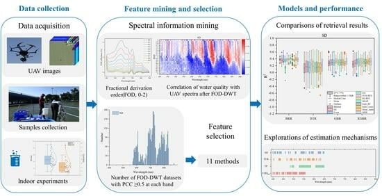
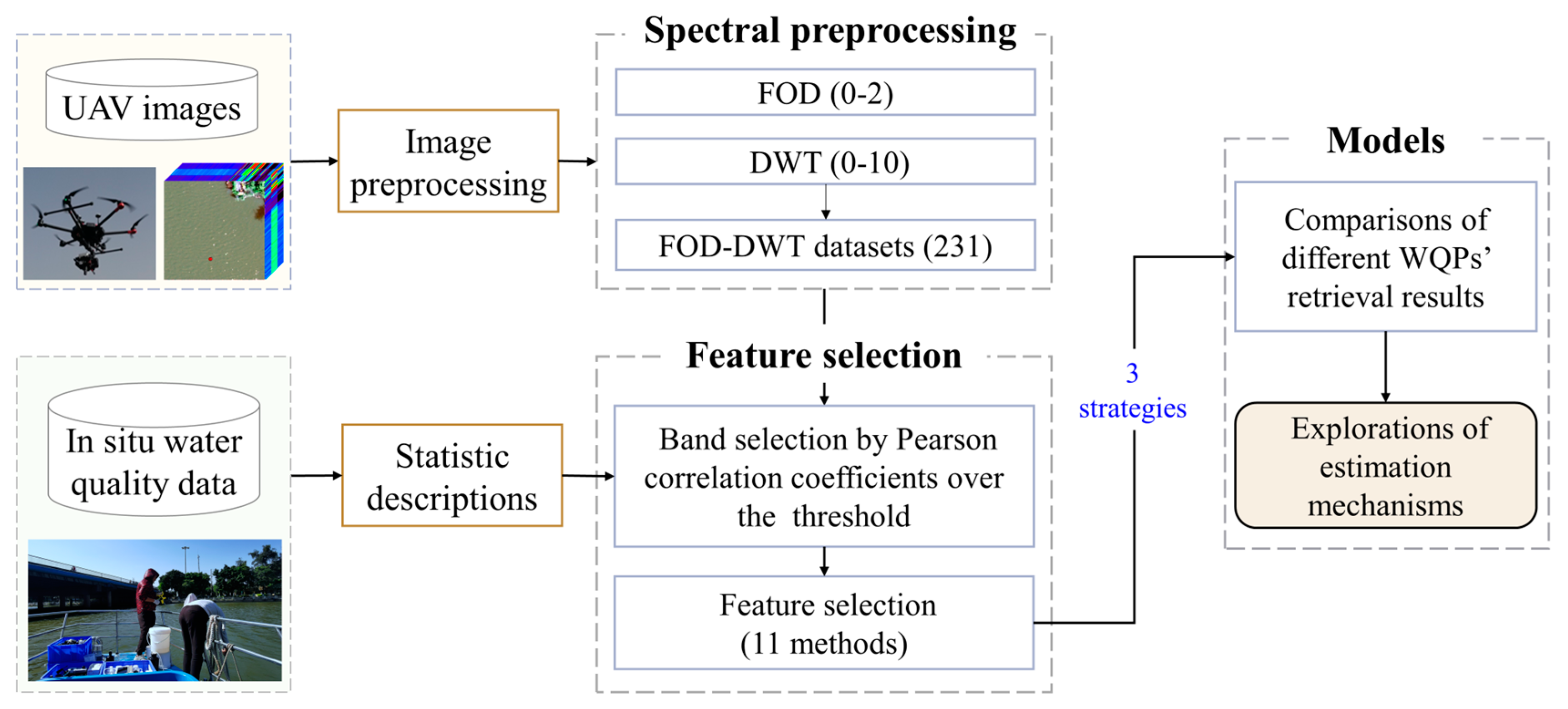
2.2. Research Framework

The research framework is illustrated in Figure 2. Initially, in Section 2.3.2, UAV images underwent image preprocessing, followed by spectral preprocessing in Section 2.4 and feature selection in Section 2.5. Furthermore, the features extracted after FOD-DWT processing were explored in Section 3.2. Subsequently, four ML regression models were adopted, and the accuracy comparisons for different WQPs were conducted under three strategies with distinct procedures in Section 3.3. Lastly, sensitive spectral bands were presented in Section 3.3.2, and the mechanisms behind the water quality inversion were analyzed in Section 4.2.

2.3. Data Acquisition

2.3.1. Water Quality Data Sampling

On 14 October 2022 and 15 October 2022, 45 water samples were collected from the locations in Figure 1a, at a depth of 0.5 m below the water surface. Most sampling points on the Huadi River were obtained by boat from the center of the river, while small rivers that were inaccessible to boats were sampled ~3 m away from the shore. Boat sampling in the narrow Kuipeng and Jiansha Rivers was impossible due to local constraints. The water depth of the two rivers was approximately 1.5–2 m, and the riverbed was not visible around the sampling points. Therefore, the UAV images recorded the reflectance of the water surface without the optical effect of the bottom interference.

Each sampling point involved the collection of five 250 mL water samples for laboratory analysis, along with two 1 L backup samples. Those samples were stored in brown light-avoiding bottles, sealed, labeled, fixed, and preserved to prevent any alterations in test results due to water quality changes during transportation. All WQPs were assayed within 3 days. SD and TUB were determined on-site by a Secchi disk and a turbidity meter, respectively. TP and COD_Mn were measured in laboratory conditions. Portable GPS devices were utilized during the sampling process to record the geographical locations accurately.

Parallel sampling was employed to ensure sampling quality. Among the 45 sampling points, 5 were selected for parallel sampling, achieving a proportion of 11.1%. Three parallel samples were taken at each point, and the final value at each point was the mean of the three parallel samples. When the relative standard deviation (RSD) in Equation (1) for each point is ≤10%, it indicates that the sampling quality meets the requirements.

$$RSD=\frac{S}{\overline{x}}\times 100\mathrm{\%}=\frac{\sqrt{\frac{{\sum }_{i=1}^n{(x_i-\overline{x})}^2}{n-1}}}{\overline{x}}\times 100\mathrm{\%}$$

(1)

where $S$ represents the standard deviation;$\overline{x}$ signifies the corresponding mean value; $n$ is the number of samples.

2.3.2. UAV Acquisition and Processing

The collection of UAV images and ground samples occurred simultaneously during the same periods (morning and afternoon), as indicated in

Table 1. UAV flight time and speed.

Flights	Time	Speed (m/s)
1	14 October 2022; 10:56–11:19	5.0
2	14 October 2022; 11:55–12:17	5.0
3	14 October 2022; 13:35–14:06	5.0
4	14 October 2022; 14:33–15:09	5.0
5	15 October 2022; 09:32–09:54	5.5
6	15 October 2022; 10:42–11:08	5.5
7	15 October 2022; 14:01–14:22	5.5
8	15 October 2022; 14:44–15:03	5.5

. The weather was clear and cloudless. Since the UAV flight time was from approximately 9 am to 3 pm, when the wind speed was actually minimal, its impact on the UAV images was very slight. The drone flew smoothly over the rivers.

The UAV system was the DJI M300 RTK, flying at an altitude of 200 m. Flight times and speeds are detailed in Table 1. The UAV was equipped with the Pika L hyperspectral camera produced by RESONON in the United States, weighing 0.6 kg. It utilizes a linear push-broom imaging method, which is highly efficient for large-scale operations. The spectral range is 400–1000 nm, encompassing 561 channels with a spectra bandwidth of 1.07 nm. Due to the weak optical reflection signals from the water surface, a binning technique [39] was employed to combine several adjacent pixels into one, thereby enhancing the pixel responsiveness and signal-to-noise ratio of the linear CCD. The spectra intervals of the final collected UAV images were 4 nm. Considering the sensor noise at both ends, spectral information within the 400–900 nm range was finally chosen. Therefore, the number of input bands for spectral preprocessing was 125. The spatial resolution of the acquired UAV images was resampled from 0.199 m to 0.2 m in ENVI 5.3, to facilitate possible subsequent comparisons with satellite images in the future. The field of view (FOV) was 17.6@17 mm. To minimize the time gap between the imaging of the UAV images and the ground sampling, the overlap between adjacent images was set to 30%. The stitched images were then examined to ensure they met the requirements. The UAV imagers covered all sampling points and approximately 12 km of river length (Figure 1b).

The data obtained directly from UAV flights are in the form of digital number (DN) values. These data require processing and stitching to obtain reflectance values. During the acquisition of the hyperspectral images, several gray standard cloths with known reflectance values of 0.1 and 0.3 were placed on the ground as calibration targets, which created a higher-frequency calibration reference. Given the flight altitude of 200 m, complex atmospheric effects can be ignored [40]. The processing workflow involved the following steps. Firstly, geometric correction and radiometric correction were conducted using MegaCube 2.9.6.3 software. Secondly, using ArcMap 10.4 for georeferencing, all images in this study were defined in the same coordinate system, namely the Universal Transverse Mercator (UTM) projection. Finally, image stitching and the generation of reflectance images were conducted based on ENVI 5.3. Each pixel can yield a complete high-resolution spectral curve. To enhance stability, the mean DN value of a 3 × 3 window corresponding to each sampling point on the image was selected as the final DN value for that point [41].

2.4. Spectral Preprocessing

First, SG smoothing was applied to reduce noise interference and achieve smoother curve transitions [14]. Then, the FOD method was employed to uncover latent spectral information, followed by the DWT to extract spectral features.

2.4.1. Fractional Order Derivation

Integer-order differentials might overlook subtle spectral information details. FOD can compute fractional-order differentials, allowing for the highlighting of differences between spectral information and minimizing spectral information loss. The FOD order range was set from 0 to 2 with a step of 0.1, resulting in 21 orders. Setting the order to 0 represents the OR, while orders of 1.0 and 2.0 correspond to the first and second derivatives, respectively. FOD is defined by the Grünwald–Letnikov method [42] as follows:

$$D^{\alpha }f\left(x\right)=\underset{h\to 0}{\lim }{h}^{-\alpha }\sum _{k=0}^{\frac{t-t_0}{h}}{(-1)}^k\frac{\Gamma (\alpha +1)}{\Gamma (k+1)\Gamma (\alpha -k+1)}f(x-kh)$$

(2)

where $f\left(x\right)$ is the reflectance of the spectra; $\alpha$ is the order; $h$ is the step size; $k$ is a constant; $t$ and $t_0$ are the upper and lower wavelength ranges of the FOD, respectively. $\Gamma \left(\gamma \right)$ is the gramm function, expressed as follows:

$$\Gamma \left(\gamma \right)={\int }_0^{\infty }\exp \left(-u\right)u^{\gamma -1}du=\left(\gamma -1\right)!$$

(3)

2.4.2. Discrete Wavelet Transform

DWT is used to extract spectral features, offering distinct advantages such as time-scale representation, multi-scale analysis, and multi-resolution analysis [16]. The DWT decomposition level was set from 0 to 10, employing the db4 mother wavelet and VisuShrink thresholding for threshold selection. The processing of DWT decomposition and reconstruction involves filtering to remove noise from high-frequency components, ultimately reconstructing various signal subbands in the spatial domain. Consequently, DWT not only eliminates noise but also simplifies the disparities in spectral bands. DWT can be defined using Equation (4) [23,43]:

$$W_f(j,k)=2^{j/2}{\int }_{-\infty }^{+\infty }f\left(t\right)\overline{\psi \left(2^{j}t-k\right)} dt=〈f\left(t\right), {\psi }_{j,k}(t)〉$$

(4)

where $W_f(j,k)$ is the $f\left(t\right)$ wavelet transform coefficient; $j$,$kϵZ$; $f\left(t\right)$ is the length of the signal sequence; ${\psi }_{j,k}(t)$ is the mother wavelet. $\overline{\psi \left(2^{j}t-k\right)}$ is the conjugate of $\psi \left(2^{j}t-k\right)$. And $〈f\left(t\right), {\psi }_{j,k}(t)〉$ represents the inner product.

2.5. Feature Selection Methods

Various feature selection methods were realized to extract distinctive spectral information. To explore suitable methods for different WQPs, this study selected a total of 11 methods, including 3 from the filter, 4 from the wrapper, 2 from the embedded, and 2 from the ensemble categories. Except for the genetic algorithms (GA), which cannot directly set the output number of bands, the amount of the optimal output feature was set to 30 to reduce data dimensionality.

In the filter methods, features are ranked based on statistical criteria such as distance, correlation, and information gain. RReliefF considers inter-feature relationships, effectively capturing the nonlinear relationships between features and output variables, thus being applied to high-dimensional and nonlinear problems [44]. Mutual information regression (MI) employs an information gain to select features and is more powerful than an F-test, which is limited to linear relationships [45].

Wrapper methods employ feature subset search algorithms, exploring possible subsets and evaluating regressor performance to identify the best feature subset. However, this approach is prone to overfitting with limited data and can be time-consuming when dealing with numerous features. GA is time-intensive [46], influenced by settings like population_size and generations. Support vector machines—RFE (SVM-RFE) and RF-RFE have a notably improved performance in vegetation [17,24] but have been scarcely used in water quality retrieval. SHapley Additive exPlanations (SHAP) combines game theory and local explanations [45], offering accurate local feature attribution, though its application in water quality retrieval has been limited.

Embedded methods incorporate optimal feature subsets into regressor construction, benefiting from a guided search during the learning process, resulting in high accuracy and lower computational costs. Lasso regression (Emb_Lasso) utilizes L1 regularization to select features, while random forest (Emb_RF) employs feature importance indices from the random forest model.

Ensemble feature selection methods aggregate predictions of multiple base models through weighted averaging, ultimately yielding the final prediction. The mean ranks (Mean_ranks) method in Equation (5) ranks the results of various feature selectors by importance, selecting the features with the highest mean value of the scores’ sum [47], seldom used in water quality inversion. The mean reciprocal ranking (MRR) in Equation (6) ranks the results of multiple feature selectors, obtaining the rank of each feature across different feature selectors. It then calculates the sum of the reciprocal ranks for each feature, with the highest-scoring feature being selected [45].

$${Mean\_rank}_i=\frac{1}{n}{\sum }_{j=1}^n{f}_{ij}$$

(5)

$${MRR}_i=\frac{1}{n}{\sum }_{j=1}^n\frac{1}{f_{ij}}$$

(6)

where $i$ is the number of bands for input spectra. $n$ is the amount of single feature selection methods (including RReliefF, MI, F-test, GA, SVM-RFE, RF-RFE, SHAP, Emb_Lasso, and Emb_RF), and n = 9. $f_{ij}$ represents the ranking assigned to feature $i$ by ranker $j$.

2.6. Modeling of WQP Inversion

Four ML models were adopted to invert these four WQPs. The Bayesian ridge regression (BRR) algorithm, used for collinear data analysis in regression, is an estimation bias that optimizes and extends traditional least squares estimation. The algorithm employs a hyperparameter that governs the regularization intensity and fully integrates this hyperparameter within the posterior distribution, utilizing a hyperprior chosen to approximate a noninformative stance. It performs better in simulating ill-conditioned data than ordinary least squares [34]. The decision tree regression (DTR) algorithm falls under the category of the supervised learning algorithms. It works for both continuous as well as categorical output variables, which consists of two steps: firstly, building a decision tree of a certain size for the training dataset; secondly, pruning the established tree using a validation dataset to select the optimal subtree that meets practical requirements [34]. The gradient boosting regression (GBR) updates the regression coefficients using only one sample point, greatly improving computational complexity [34] and time consumption. An XGBoost regression (XGBR) constructs multiple weak estimators on the dataset and aggregates the modeling results of all weak estimators to achieve better regression performance than a single model [40]. An XGBR strikes a balance between model performance and computational speed, demonstrating advantages in small-volume sample data [22]. Some studies [32,33] have shown good performance in water quality prediction using an XGBR, even based on the small sample size.

The ‘train_test_split’ method provided by Scikit-learn [48] was employed to randomly divide the total samples into 70% training samples (31) and 30% validation samples (14). To explore the impact of the spectral preprocessing and feature selection methods, 3 strategies were designed (

Table 2. Regression strategies for WQPs combining different treatment procedures.

Procedures	FOD-DWT Processing	Select Bands by PCC > 0.5	Feature Selection by 11 Methods	Calculation Accuracies
Strategy 1				√
Strategy 2			√	√
Strategy 3	√	√	√	√

). The OR data was processed using FOD and DWT, resulting in 231 different datasets with combinations of FOD and DWT values. The Pearson correlation coefficient (PCC) between each FOD-DWT dataset and each WQP was calculated, where a higher value indicates a stronger correlation [40].

2.7. Accuracy Evaluation

The performance of the regression models was assessed using four metrics. The first metric is the coefficient of determination (R²) in Equation (7), which explains the variance score of a regression model, with values ranging from 0 to 1. A value closer to 1 indicates a more stable model, while a lower value suggests poorer performance.

$$R^2=1-\frac{{\sum }_{i=1}^n{(y_i-\widehat{y_i})}^2}{{\sum }_{i=1}^n{(y_i-\overline{y_i})}^2}$$

(7)

where n is the number of samples.$y_i$ and $\widehat{y_i}$ are the actual value and corresponding predicted value of a parameter for the sample $i$, respectively. $\overline{y_i}$ represents the average value of the actual values of the parameter.

The root-mean-square error (RMSE) is defined in Equation (8) as sensitive to both large and small errors, making it a reflection of the accuracy of predictions [8]. The mean absolute error (MAE) in Equation (9) is used to assess the degree of closeness between the predicted values and the actual data. The mean absolute percentage error (MAPE) takes into account the relative error as a percentage of the actual values in Equation (10), which helps address the issue of neglecting small-scale errors. The smaller RMSE, MAE and MAPE indicate a better fitting performance.

$$RMSE=\sqrt{\frac{{\sum }_{i=1}^n{(y_i-\widehat{y_i})}^2}{n}}$$

(8)

$$MAE=\frac{1}{n}\sum _{i=0}^{n-1}\left|y_i-\widehat{y_i}\right|$$

(9)

$$MAPE=\frac{1}{n}\sum _{i=0}^{n-1}\frac{\left|y_i-\widehat{y_i}\right|}{max(ϵ, {|y}_i|)}$$

(10)

where $ϵ$ is an arbitrary small, yet positive number to avoid undefined results when $y$ is 0.

3. Results

3.1. Descriptive Characteristics

3.1.1. Descriptive Characteristics

Firstly, the determination of WQPs met the requirements of quality control in Section 2.3.1, namely the RSD of each WQP at these parallel sampling points ranged from 0% to 9%. Then, the fluctuation of the water quality data was depicted using a box plot (Figure 3). The SD showed relatively large variations. In the TUB, a few extreme values were contributing to a higher standard deviation (

Table 3. Statistical results of the WQPs.

Parameters	Unit	Min	Max	Mean	Std	Skew	Kurtosis
SD	cm	11.00	90.00	47.20	19.90	0.58	−0.37
TUB	NTU	7.10	75.00	24.76	17.40	1.49	2.04
TP	mg/L	0.09	0.49	0.19	0.08	1.64	4.04
CODMn	mg/L	2.30	6.80	4.32	1.06	0.64	−0.11

). This is attributed to rapid changes in suspended solid concentrations due to the opening and closing of the Huadi River sluice gates during sampling, causing the observed extreme values.

According to the “Environmental Quality Standards for Surface Water” of China, two sampling points have TP values exceeding 0.3 mg/L, referred to as Class IV water, while the rest of the samples are classified as Class III or better. The COD_Mn content in all samples is below 10 mg/L, with only a small portion of Class IV exceeding 6 mg/L.

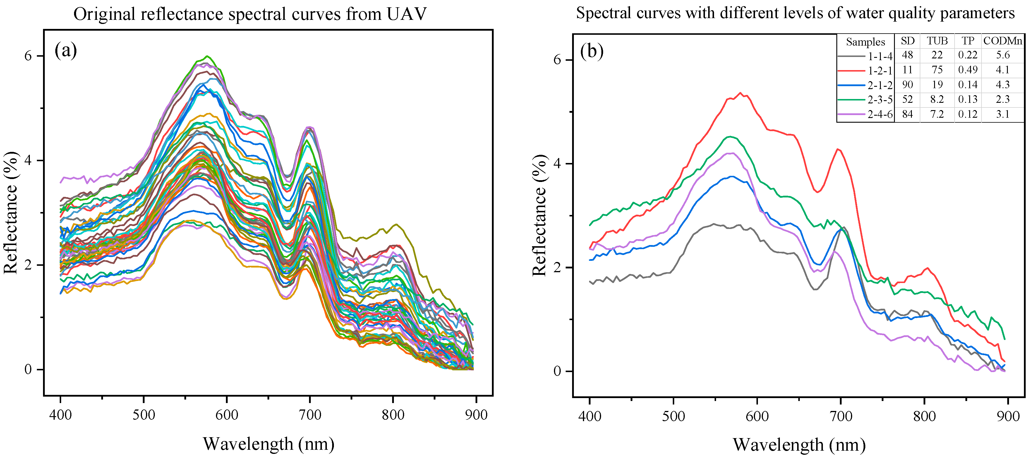
3.1.2. Spectral Characteristics

The spectra of each ground sampling point were extracted from the UAV images and plotted as continuous curves with 125 bands (Figure 4a). Overall, the image reflectance ranged below 6%, with higher reflectance observed in 500–700 nm. The spectral reflectance between 550–600 nm was significantly higher. Prominent peaks appeared around 550 nm and 700 nm, while a distinct trough was visible around 675 nm. After 800 nm, there was a noticeable decrease in reflectance.

Varying water constituents make differences in the spectral curves. Five curves representing different WQP concentrations were selected for comparison (Figure 4b). With increasing TUB, spectral reflectance increased notably. However, for non-optically active parameters like TP and COD_Mn, there was not a clear pattern of significant spectral differences with varying concentrations. Curves like 1-2-1, 2-3-5, and 2-4-6 were from the upstream section near the northern gate of the Huadi River, the lower section of the Huadi River, and near the southern gate of the Huadi River, respectively. Curve 1-1-4 was from the Guangfo River, sampled on 14 October 2022, but it showed a smoother peak in the 550–600 nm range and an overall lower reflectance. Curve 2-1-2 was from the Jiansha River, showing no distinct difference from spectral curves on the Huadi River. Additionally, variations in the spectral features among sampling points of the Huadi River and small rivers like the Jiansha River were observed.

3.2. Features of Preprocessed Spectra

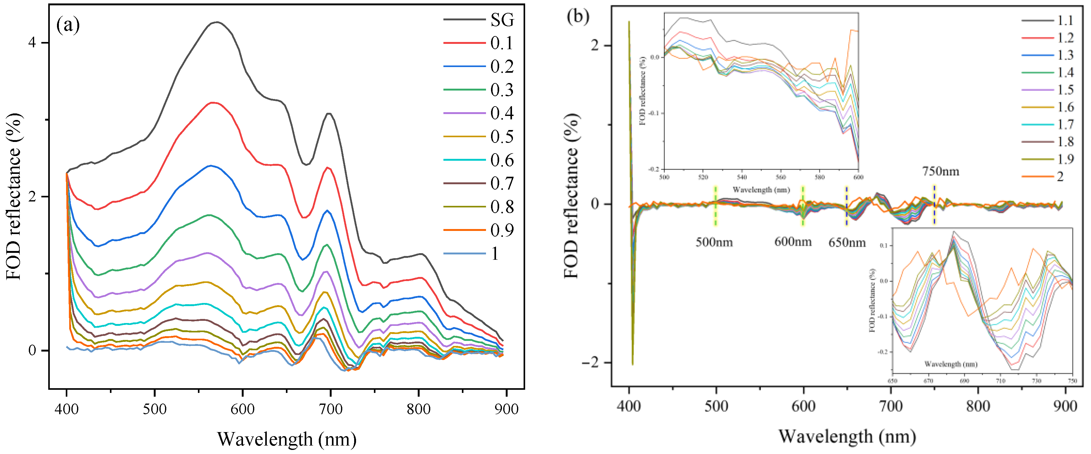
3.2.1. Spectral Features with FOD

The mean spectral reflectance curves based on the UAV images were employed to investigate the influence of the FOD processing. In Figure 5a, as the order increased, the FOD reflectance gradually decreased. However, all curves still exhibited similar trends, particularly evident in the (0.1, 1.0) range of orders. As the order increases from 0.6 to 2.0, the fluctuations in the FOD-processed curves become more pronounced, with an increasing number of peaks and valleys appearing on the curves. Specifically, when the order was set within (1.1, 2.0), the FOD-processed curves showed increased distinct features between 500–600 nm and 650–750 nm (Figure 5b). This may offer more specific information for the identification of WQPs. The closer spacing of orders in FOD provided more subtle spectral features.

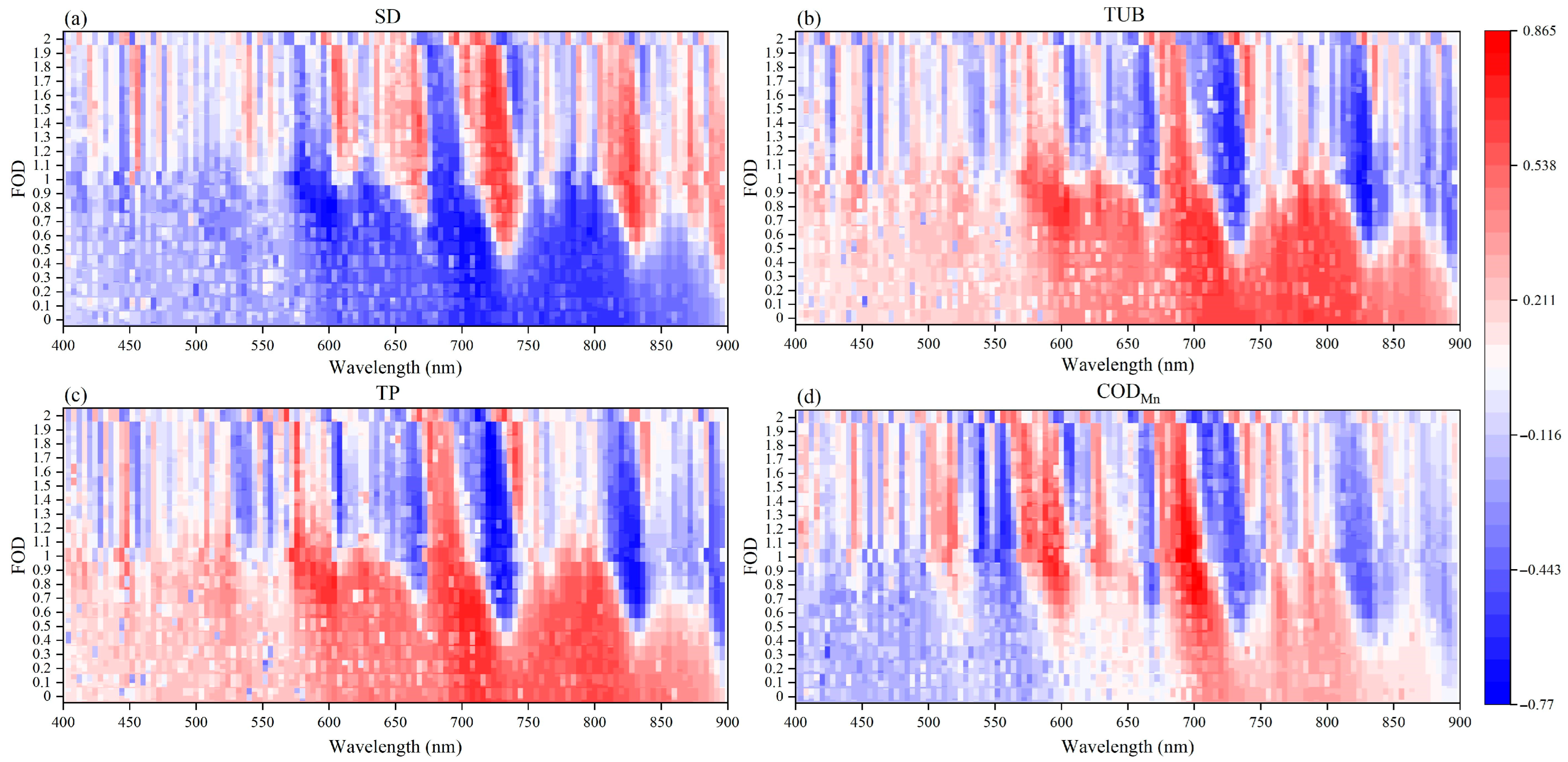
3.2.2. Correlation Analysis between WQPs and Preprocessed Spectra

The selection of a spectral range between 400 to 900 nm in Section 2.3.2 helped to neglect the peripheral spectral data prone to noise, resulting in small changes after the DWT processing [23]. Therefore, a correlation analysis was adopted to further explore the effects of the FOD-DWT processing. With the combinations of FOD orders (0–2.0) and DWT levels (0–10), a total of 231 sets of FOD-DWT preprocessed spectra were obtained. The PCCs between the WQPs and the 231 FOD-DWT datasets were computed and compared on different UAV bands (Figure 6).

Taking TUB as an example (Figure 6b), the exploration of spectral features was conducted. For the OR data, high correlations were concentrated between 680–844 nm. For the FOD-DWT processed spectra, the number of bands with a higher PCC increased, and the correlation became stronger when the orders were set as 0.6, 0.7, and 0.8. The processing with FOD and DWT highlighted the spectral features of WQPs. However, as the FOD order gradually increased and surpassed 1.3, the number of bands with high correlations decreased, suggesting that the spectra might be less stable. Furthermore, as illustrated in Figure 6, the PCC did not show significant changes with variations in DWT levels, indicating a limited role of DWT in improving correlation.

The number of FOD-DWT datasets with which PCCs exceeded the threshold of 0.5 for each wavelength $\mathrm{i}(400\le \mathrm{i}\le 900)$ was tabulated and denoted as ${\mathrm{N}\mathrm{u}\mathrm{m}}_{\mathrm{i}}$ ($0\le {\mathrm{N}\mathrm{u}\mathrm{m}}_{\mathrm{i}}\le 231$) (Figure 7). A higher value of ${\mathrm{N}\mathrm{u}\mathrm{m}}_{\mathrm{i}}$ at wavelength $\mathrm{i}$ implies a greater possibility of reflecting features of WQPs. For SD, at 720 nm, 724 nm and 728 nm, ${\mathrm{N}\mathrm{u}\mathrm{m}}_{\mathrm{i}}$ counted 176, 173, and 165, respectively, which underscored high correlations. For SD, TUB, and TP, the ${\mathrm{N}\mathrm{u}\mathrm{m}}_{\mathrm{i}}$ was predominantly highest at 572–612 nm, 680–740 nm, and 760–832 nm, respectively. This implies a heightened sensitivity of these wavelength intervals to the three aforementioned WQPs. In contrast, for COD_Mn, the range of 536–608 nm also exhibited a significant ${\mathrm{N}\mathrm{u}\mathrm{m}}_{\mathrm{i}}$, while no datasets demonstrated a PCC exceeding 0.5 after 732 nm. COD_Mn exhibited distinctive characteristics, potentially rendering it more advantageous for WQP inversion.

3.3. Regression Results

3.3.1. Comparisons of Different Strategies

The optimal accuracies of the regression models based on the validation samples under the three strategies are compared in

Table 4. Regression accuracies of the WQPs obtained by different strategies. OR, OR_FS, and FOD_DWT_231 correspond to strategies 1, 2, and 3, respectively. The bold ones are the highest R² for each WQP based on a certain strategy.

WQPs	Models	OR				OR_FS				FOD_DWT_231
		R2	RMSE	MAPE	MAE	R2	RMSE	MAPE	MAE	R2	RMSE	MAPE	MAE	FOD	DWT
SD	BRR	0.45	18.19	0.36	14.77	0.47	17.72	0.33	14.00	0.65	14.47	0.25	10.66	1.6	4
	DTR	0.45	18.11	0.38	14.21	0.53	16.70	0.38	13.29	0.68	13.73	0.32	10.86	1.6	5
	GBR	0.50	17.31	0.35	12.90	0.56	16.22	0.34	12.46	0.62	15.01	0.36	11.58	1.6	6
	XGBR	0.41	18.85	0.35	13.44	0.54	16.49	0.33	12.06	0.64	14.62	0.34	10.86	1.6	4
TUB	BRR	0.61	12.84	0.37	8.25	0.70	11.28	0.31	7.11	0.55	13.80	0.32	8.29	0.8	9
	DTR	0.49	14.72	0.21	7.59	0.69	11.50	0.16	6.00	0.90	6.50	0.17	4.07	2	4
	GBR	0.46	15.21	0.38	9.13	0.52	14.36	0.30	8.67	0.65	12.14	0.23	6.93	1.2	6
	XGBR	0.19	18.55	0.33	11.02	0.40	15.95	0.24	8.40	0.72	10.87	0.23	7.08	0.5	0
TP	BRR	0.27	0.09	0.26	0.05	0.44	0.08	0.27	0.05	0.50	0.07	0.19	0.04	0.3	5
	DTR	−0.17	0.11	0.43	0.07	0.74	0.05	0.25	0.04	0.70	0.06	0.28	0.04	0	5
	GBR	0.18	0.09	0.36	0.06	0.32	0.08	0.33	0.05	0.51	0.07	0.25	0.05	1.5	1
	XGBR	0.35	0.08	0.31	0.05	0.51	0.07	0.31	0.05	0.59	0.07	0.26	0.04	1.2	2
CODMn	BRR	0.88	0.36	0.06	0.28	0.87	0.36	0.07	0.29	0.94	0.26	0.05	0.21	1.7	5
	DTR	0.64	0.61	0.12	0.46	0.82	0.43	0.09	0.35	0.92	0.29	0.05	0.24	0.7	2
	GBR	0.82	0.43	0.08	0.32	0.90	0.33	0.07	0.27	0.94	0.24	0.04	0.17	0.8	9
	XGBR	0.72	0.53	0.11	0.43	0.83	0.41	0.06	0.28	0.96	0.20	0.04	0.15	1.8	6

.

For Strategy 1, OR data was used as the input of the regression models, and the precision for the first three parameters was relatively low. The maximum R² value for SD lay between 0.41 and 0.50, while TUB’s maximum R² ranged from 0.19 to 0.61, indicating an inadequate stability in precision. The accuracy for TP was notably deficient, reaching a maximum of only 0.27. Notably, the BRR model exhibited higher precision in predicting TUB and COD_Mn. An occasional negative R² for TP with the DTR model possibly resulted from small sample sizes and inadequate model fitting.

From the results of Strategy 2, regression models with feature selection significantly enhanced regression performance for all four WQPs. Except for COD_Mn with BRR, the precision based on feature-selection-treated spectral data surpassed that of the OR data. For instance, TP achieved a maximum R² of 0.74, while COD_Mn’s peak accuracy reached 0.90. Regarding SD, the XGBR model showed the most substantial improvement escalating from 0.41 to 0.54, marking a 34.3% enhancement. For TUB, XGBR’s improvement was equally significant, ascending from 0.19 to 0.40, representing a 110% increase. Notably, for TP, the DTR model exhibited the highest R², 0.74. As for COD_Mn, DTR achieved the most considerable enhancement, rising from 0.64 to 0.82, a 27.9% increment.

Results after FOD-DWT processing exhibited relatively higher precision. In Table 4, the DTR model attained the highest relative R² (0.68, 0.90, 0.70 for SD, TUB, and TP, respectively). For COD_Mn, the XGBR model achieved the best precision (R² = 0.96). For almost all FOD and DWT combinations that achieved the highest R², the FOD order took on fractional values and the DWT level was non-zero. That underscored the utility of the composite processing involving FOD, DWT, and feature selection in enhancing regression precision for WQPs.

To investigate the impact of feature selection methods on the regression performance of Strategy 3, the precision of the 231 FOD-DWT-processed datasets was further computed and analyzed (Figure 8). For each regression model, the statistical R² results of 11 different feature selection methods were shown in each subfigure. Despite DTR achieving the highest R² values for the first three WQPs (Table 4), the majority of the 231 results exhibited notable fluctuations, with an average R² lower than that of the other models (Figure 8), indicating a lack of stability. In general, the results of the BRR model appeared to be more stable, with an average precision higher than that of other ML models. Additionally, according to the best R² in Table 4, RRF-RFE, GA, MI, and MRR were identified as the optimal feature selection methods for the four WQPs. For TUB, the GA feature selection method demonstrated relatively better overall performance. However, for the other WQPs, the optimal feature selection method varied under different spectral preprocessing methods and regression models. Relief, RF-RFE, and MRR performed well across multiple WQPs and regression models. This emphasizes the necessity of considering appropriate methods to filter features.

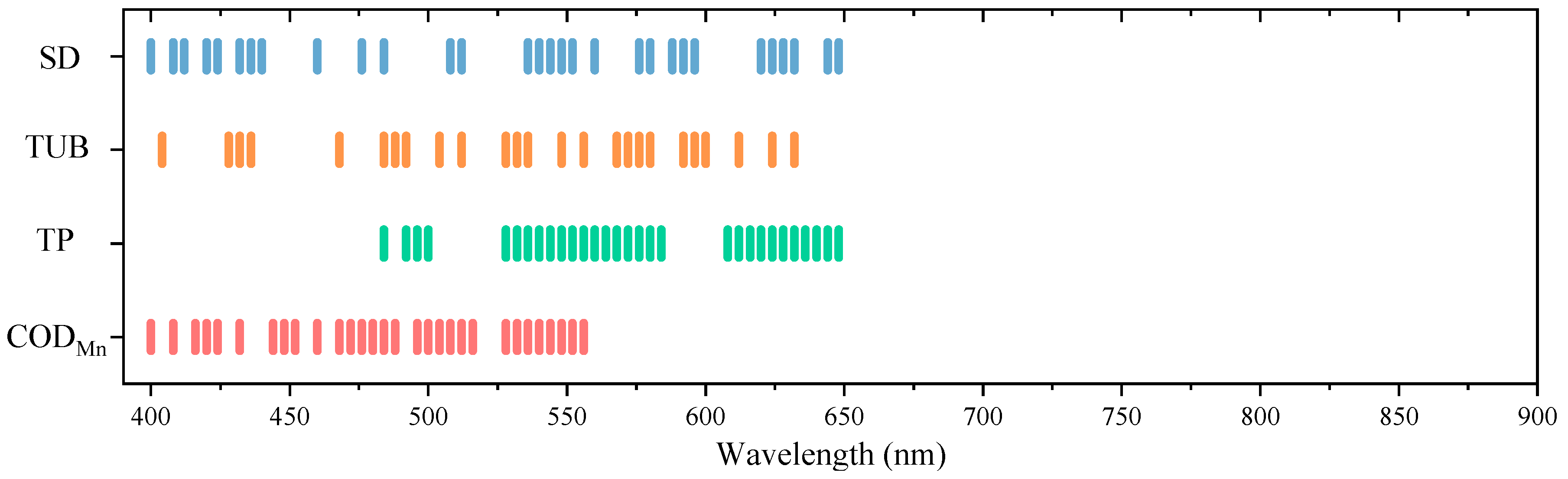
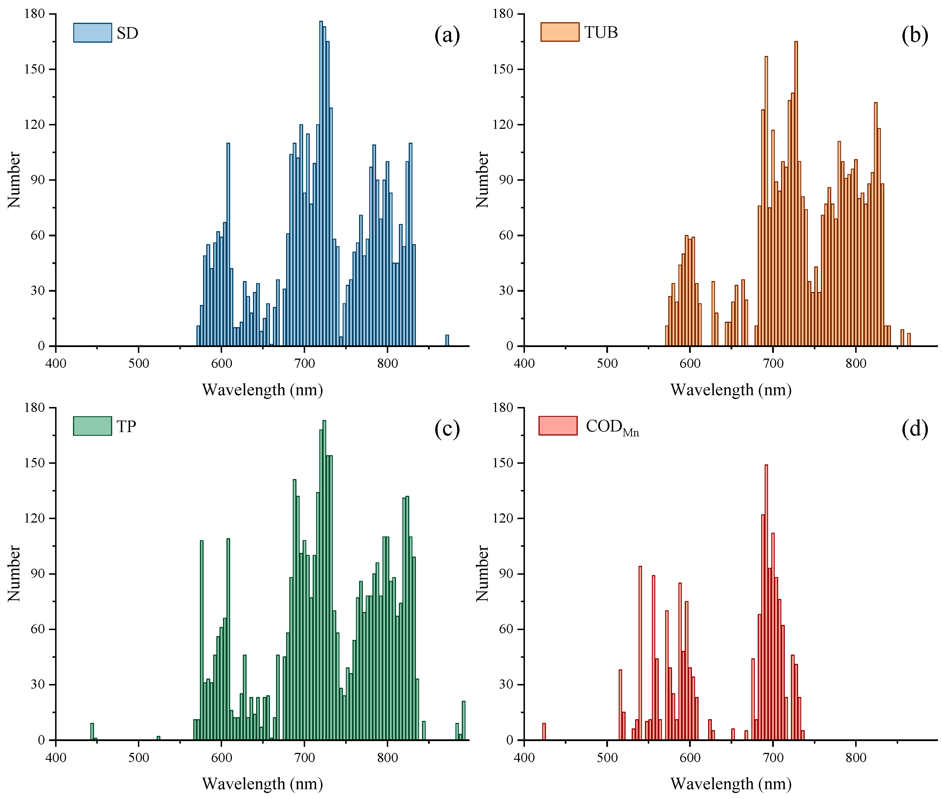
3.3.2. Sensitive Spectral Bands of WQPs

To further explore the sensitive spectral bands for each WQP, Figure 9 was employed for presentation based on the maximum R² values obtained from Strategies 3 in Table 4. Sensitive bands varied for different WQPs. For optical sensitive parameters, namely SD and TUB, the sensitive bands were primarily distributed between 400 nm and 650 nm. As for TP, the sensitive bands were situated between 484–500 nm, 528–584 nm, and 608–648 nm. COD_Mn’s sensitive bands were concentrated more in the range of 400 nm to 560 nm. Notably, for the TUB with 25 sensitive bands, the actual amount was noticeably reduced due to filtering using the PCC > 0.5 in Section 2.6, potentially falling below 30.

4. Discussion

4.1. Analysis of Regression Performance

The combination of FOD and DWT for spectral preprocessing has improved the accuracy of WQP inversion. Extending FOD from an integer order to a non-integer order enables the extraction of more detailed spectral information from hyperspectral data [23]. Moreover, DWT was employed to remove high-frequency noise. As depicted in Figure 4, the complexity and diversity of urban rivers [6] made it challenging to discern a clear relationship between the original hyperspectral data and the concentrations of WQPs directly. However, the correlation between the spectra processed by FOD-DWT and the WQPs had been significantly enhanced in Figure 6. Despite the absence of explicit physical interpretations, the 0.1 step in FOD proves instrumental in revealing finer-grained information [8]. In Figure 5b, distinct curve patterns were unveiled for orders > 1. Some studies suggested that spectra based on high FOD orders (≥1) might be influenced by inherent spectral noise [16]. However, the highest accuracies were achieved with FOD orders > 1 for SD, TUB, and COD_Mn in Table 4, suggesting favorable outcomes. In conclusion, the combination of FOD and DWT had a good effect on the feature mining of non-optical active parameters via remote sensing techniques.

Furthermore, some studies [46] selected sensitive spectral bands based solely on the mean PCCs of a band after DWT processing. However, as correlations can exist between hyperspectral bands, relying solely on correlation for sensitive band selection may lack reliability. In this study, taking TP as an example, a heatmap (Figure 10) illustrated the maximum and average of the PCCs across different FOD and DWT values. The use of average PCCs in Figure 10b might obscure the prominently correlated spectral information reflected in Figure 10a. To ensure that the maximum PCC was not ignored, the correlation of all bands in each FOD-DWT combination was considered, and the bands with correlations greater than 0.5 (Figure 7) were then selected as inputs for the regression models with feature selection.

Feature selection methods have played a significant role in extracting sensitive information. In Figure 8, the advantages of those methods varied for different WQPs and regression models. The RFE algorithm can reduce redundant information in hyperspectral data, effectively improving model efficiency [16]. For TUB, the GA method outperformed other algorithms, compensating for the model’s slow convergence and susceptibility to optimal local solutions [22]. Moreover, the significant superiority of the ensemble model was only evident in the COD_Mn inversion. This indicates the continued necessity of integrating actual water quality data and preprocessing to select appropriate feature selection approaches for better regression performance.

Furthermore, the most suitable regression models differ for distinct WQPs [30]. Both DTR and XGBR are suitable for small sample size data. DTR’s learning relies on a greedy algorithm, optimizing local optimal nodes to achieve overall optimization, which does not guarantee the return of a global optimal result [24]. In Figure 8, although the DTR model lacked stability and indicated the risk of overfitting, it could fully exploit regression prediction potential. In contrast, XGBR incorporates regularization techniques to reduce overfitting, enhancing generalization capabilities and resulting in more excellent performance, but relatively conservative results where specific extreme values might not be precisely estimated [49]. Compared with published articles [30,50], the regression accuracy of the COD_Mn in this paper was relatively higher. Therefore, it is crucial to select appropriate models based on actual WQPs.

4.2. Exploration of WQP Estimation Mechanisms

Different spectral preprocessing and feature selection methods result in distinct sensitive spectral features. The sensitive bands for SD were predominantly distributed within 400–650 nm in Figure 9. Previous studies have indicated that the most correlated spectral bands for TUB are the blue bands within 400–500 nm [51] and the near-infrared band within 720–850 nm [50], with the optimal sensitive bands at 808 nm, 850 nm, and 880 nm [52]. In Figure 9, the sensitive bands corresponding to the optimal WQP inversion fell within the 404–635 nm range, consistent with previous research [51] and encompassed some spectral characteristics specific to the study area’s rivers.

For TP and COD_Mn, there are no apparent spectral curve features. Nonetheless, ML methods can identify highly correlated bands. Within the range of 450 to 630 nm, a strong positive correlation existed between the phosphorus concentration and spectral reflectance [36]. TP primarily originates from wastewater discharges from production and daily life, and an increase in its concentration may stimulate algal growth, subsequently elevating the chlorophyll-a concentration and leading to decreased SD [53]. For TP, the sensitive bands were within the ranges of 440–485 nm, 688–730 nm, and 760–832 nm in Figure 9. Hence, variations in the TP concentration can also impact the optical properties of water bodies.

4.3. Implications and Limitations

This study proposes a comprehensive ML-based framework for WQP inversion by comparing different modeling strategies. Initially, the combination of FOD and DWT was employed to unearth spectral information. To address the issue of weak spectral signatures corresponding to WQPs, this framework makes several contributions. Initially, it utilizes a combination of FOD-DWT processing to deeply mine potential spectral information and employs refined feature selection to identify valuable features while reducing computational costs. Subsequently, by selecting ML models tailored to different WQPs, it specifically enhances inversion accuracies. Furthermore, various feature selection methods were utilized to filter sensitive features, which were obtained in conjunction with the best regression model for each WQP. Although the sample size in this study remains small, the construction of a water quality inversion framework, based on the thorough mining and extraction of spectral features and the selection of suitable ML models, significantly improves the prediction accuracy of WQPs, offering insights into WQP inversion with UAV hyperspectral images under limited sample sizes.

Moreover, achieving the highest precision for the four WQPs requires suitable feature selection and ML models. Differences between algorithms best suited for optically active parameter inversion versus non-optically active parameter inversion should be considered by employing diverse algorithms for constructing inversion models [30]. Furthermore, despite the instability of the inversion results from the DTR model, it had the potential to provide superior accuracy exploration over other methods. Lastly, the revelation of sensitive spectral bands for different WQPs will contribute to combining drone hyperspectral data and satellite images for WQP monitoring [54,55]. UAV hyperspectral images will facilitate the rapid acquisition of water quality in urban rivers, supporting pollution source tracing and health protection [6,22].

Nevertheless, there are some limitations in this paper. Firstly, the limited volume of samples might result in unstable outcomes or overfitting. More in situ samples are crucial for establishing highly applicable and accurate water quality inversion models [30]. Secondly, considering that the majority of rivers in this area are influenced by tides, like the operation of the north and south gates of the Huadi River based on the tidal patterns of the Pearl River, transient turbidity events resulting from abrupt mixing could potentially impact spectral patterns and the assessment of SD and TUB values. Additionally, constructing models solely with a single ML algorithm might lead to instability and estimation errors [11]. Integrative ML models [56] and DL algorithms [10] offer alternative possibilities.

Future exploration should include the further optimization of spectral preprocessing and feature extraction methods, the investigation of new inversion algorithms such as neural network models with DL methods, and the expansion of the sample database to encompass a broader range of water quality conditions and riverine contexts. Moreover, considering the sensitivity differences of various WQPs to algorithms, future research should focus more on the choice and customization of algorithms, as well as the precise identification and application of sensitive spectral bands.

5. Conclusions

This study demonstrates that combining spectral preprocessing through FOD and DWT for hyperspectral image denoising, along with feature selection to filter sensitive features, was effective in improving the accuracy of WQP estimation. Using the FOD-DWT processed spectral data as input, the DTR model showed promising potential for WQP inversion. The proper selection of feature extraction methods and ML regression models based on the WQPs’ spectral characteristics and available sampling data is crucial for achieving higher regression precision. Based on the UAV-borne hyperspectral images, an effective ML-based framework is presented for the WQP retrieval of rivers in highly urbanized areas.

References

1. Giri, S. Water quality prospective in Twenty First Century: Status of water quality in major river basins, contemporary strategies and impediments: A review. Environ. Pollut. 2021, 271, 116332. [Google Scholar] [CrossRef]
2. Wang, S.; Shen, M.; Liu, W.; Ma, Y.; Shi, H.; Zhang, J.; Liu, D. Developing remote sensing methods for monitoring water quality of alpine rivers on the Tibetan Plateau. GISci. Remote Sens. 2022, 59, 1384–1405. [Google Scholar] [CrossRef]
3. Zhang, Y.; Shi, K.; Sun, X.; Zhang, Y.; Li, N.; Wang, W.; Zhou, Y.; Zhi, W.; Liu, M.; Li, Y.; et al. Improving remote sensing estimation of Secchi disk depth for global lakes and reservoirs using machine learning methods. GISci. Remote Sens. 2022, 59, 1367–1383. [Google Scholar] [CrossRef]
4. Jia, M.; Li, F.; Zhang, Y.; Wu, M.; Li, Y.; Feng, S.; Wang, H.; Chen, H.; Ju, W.; Lin, J.; et al. The Nord Stream pipeline gas leaks released approximately 220,000 tonnes of methane into the atmosphere. Environ. Sci. Ecotechnol. 2022, 12, 100210. [Google Scholar] [CrossRef]
5. Cillero Castro, C.; Domínguez Gómez, J.A.; Delgado Martín, J.; Hinojo Sánchez, B.A.; Cereijo Arango, J.L.; Cheda Tuya, F.A.; Díaz-Varela, R. An UAV and Satellite Multispectral Data Approach to Monitor Water Quality in Small Reservoirs. Remote Sens. 2020, 12, 1514. [Google Scholar] [CrossRef]
6. Cai, J.; Meng, L.; Liu, H.; Chen, J.; Xing, Q. Estimating Chemical Oxygen Demand in estuarine urban rivers using unmanned aerial vehicle hyperspectral images. Ecol. Indic. 2022, 139, 108936. [Google Scholar] [CrossRef]
7. Zhou, X.; Liu, C.; Akbar, A.; Xue, Y.; Zhou, Y. Spectral and Spatial Feature Integrated Ensemble Learning Method for Grading Urban River Network Water Quality. Remote Sens. 2021, 13, 4591. [Google Scholar] [CrossRef]
8. Wang, J.; Shi, T.; Yu, D.; Teng, D.; Ge, X.; Zhang, Z.; Yang, X.; Wang, H.; Wu, G. Ensemble machine-learning-based framework for estimating total nitrogen concentration in water using drone-borne hyperspectral imagery of emergent plants: A case study in an arid oasis, NW China. Environ. Pollut. 2020, 266, 115412. [Google Scholar] [CrossRef]
9. Giles, A.B.; Correa, R.E.; Santos, I.R.; Kelaher, B. Using multispectral drones to predict water quality in a subtropical estuary. Environ. Technol. 2024, 45, 1300–1312. [Google Scholar] [CrossRef]
10. Zhao, C.; Li, M.; Wang, X.; Liu, B.; Pan, X.; Fang, H. Improving the accuracy of nonpoint-source pollution estimates in inland waters with coupled satellite-UAV data. Water Res. 2022, 225, 119208. [Google Scholar] [CrossRef]
11. Cheng, Q.; Xu, H.; Fei, S.; Li, Z.; Chen, Z. Estimation of Maize LAI Using Ensemble Learning and UAV Multispectral Imagery under Different Water and Fertilizer Treatments. Agriculture 2022, 12, 1267. [Google Scholar] [CrossRef]
12. Bussières, S.; Kinnard, C.; Clermont, M.; Campeau, S.; Dubé-Richard, D.; Bordeleau, P.-A.; Roy, A. Monitoring Water Turbidity in a Temperate Floodplain Using UAV: Potential and Challenges. Can. J. Remote Sens. 2022, 48, 565–574. [Google Scholar] [CrossRef]
13. Khan, M.J.; Khan, H.S.; Yousaf, A.; Khurshid, K.; Abbas, A. Modern Trends in Hyperspectral Image Analysis: A Review. IEEE Access 2018, 6, 14118–14129. [Google Scholar] [CrossRef]
14. Kwon, S.; Seo, I.W.; Noh, H.; Kim, B. Hyperspectral retrievals of suspended sediment using cluster-based machine learning regression in shallow waters. Sci. Total Environ. 2022, 833, 155168. [Google Scholar] [CrossRef]
15. Laamrani, A.; Berg, A.A.; Voroney, P.; Feilhauer, H.; Blackburn, L.; March, M.; Dao, P.D.; He, Y.; Martin, R.C. Ensemble Identification of Spectral Bands Related to Soil Organic Carbon Levels over an Agricultural Field in Southern Ontario, Canada. Remote Sens. 2019, 11, 1298. [Google Scholar] [CrossRef]
16. Meng, X.; Bao, Y.; Ye, Q.; Liu, H.; Zhang, X.; Tang, H.; Zhang, X. Soil Organic Matter Prediction Model with Satellite Hyperspectral Image Based on Optimized Denoising Method. Remote Sens. 2021, 13, 2273. [Google Scholar] [CrossRef]
17. Pullanagari, R.R.; Kereszturi, G.; Yule, I. Integrating Airborne Hyperspectral, Topographic, and Soil Data for Estimating Pasture Quality Using Recursive Feature Elimination with Random Forest Regression. Remote Sens. 2018, 10, 1117. [Google Scholar] [CrossRef]
18. Li, Z.; Chen, Z.; Cheng, Q.; Duan, F.; Sui, R.; Huang, X.; Xu, H. UAV-Based Hyperspectral and Ensemble Machine Learning for Predicting Yield in Winter Wheat. Agronomy 2022, 12, 202. [Google Scholar] [CrossRef]
19. Harringmeyer, J.P.; Ghosh, N.; Weiser, M.W.; Thompson, D.R.; Simard, M.; Lohrenz, S.E.; Fichot, C.G. A hyperspectral view of the nearshore Mississippi River Delta: Characterizing suspended particles in coastal wetlands using imaging spectroscopy. Remote Sens. Environ. 2024, 301, 113943. [Google Scholar] [CrossRef]
20. Stroud, M.K.; Allen, G.H.; Simard, M.; Jensen, D.; Gorr, B.; Selva, D. Optimizing Satellite Mission Requirements to Measure Total Suspended Solids in Rivers. IEEE Trans. Geosci. Remote Sens 2024, 62, 1–9. [Google Scholar] [CrossRef]
21. Arango, J.G.; Nairn, R.W. Prediction of Optical and Non-Optical Water Quality Parameters in Oligotrophic and Eutrophic Aquatic Systems Using a Small Unmanned Aerial System. Drones 2020, 4, 1. [Google Scholar] [CrossRef]
22. Chen, B.; Mu, X.; Chen, P.; Wang, B.; Choi, J.; Park, H.; Xu, S.; Wu, Y.; Yang, H. Machine learning-based inversion of water quality parameters in typical reach of the urban river by UAV multispectral data. Ecol. Indic. 2021, 133, 108434. [Google Scholar] [CrossRef]
23. Liu, J.; Ding, J.; Ge, X.; Wang, J. Evaluation of Total Nitrogen in Water via Airborne Hyperspectral Data: Potential of Fractional Order Discretization Algorithm and Discrete Wavelet Transform Analysis. Remote Sens. 2021, 13, 4643. [Google Scholar] [CrossRef]
24. Hu, Y.; Xu, L.; Huang, P.; Luo, X.; Wang, P.; Kang, Z. Reliable Identification of Oolong Tea Species: Nondestructive Testing Classification Based on Fluorescence Hyperspectral Technology and Machine Learning. Agriculture 2021, 11, 1106. [Google Scholar] [CrossRef]
25. Hu, W.; Liu, J.; Wang, H.; Miao, D.; Shao, D.; Gu, W. Retrieval of TP Concentration from UAV Multispectral Images Using IOA-ML Models in Small Inland Waterbodies. Remote Sens. 2023, 15, 1250. [Google Scholar] [CrossRef]
26. Prati, R.C. Combining feature ranking algorithms through rank aggregation. In Proceedings of the 2012 International Joint Conference on Neural Networks (IJCNN), Brisbane, Australia, 10–15 June 2012; pp. 1–8. [Google Scholar]
27. Prior, E.M.; O’Donnell, F.C.; Brodbeck, C.; Donald, W.N.; Runion, G.B.; Shepherd, S.L. Measuring High Levels of Total Suspended Solids and Turbidity Using Small Unoccupied Aerial Systems (sUAS) Multispectral Imagery. Drones 2020, 4, 54. [Google Scholar] [CrossRef]
28. Tang, Y.; Pan, Y.; Zhang, L.; Yi, H.; Gu, Y.; Sun, W. Efficient Monitoring of Total Suspended Matter in Urban Water Based on UAV Multi-spectral Images. Water Resour. Manag. 2023, 37, 2143–2160. [Google Scholar] [CrossRef]
29. Li, Z.; Liu, H.; Zhang, C.; Fu, G. Generative adversarial networks for detecting contamination events in water distribution systems using multi-parameter, multi-site water quality monitoring. Environ. Sci. Ecotechnol. 2023, 14, 100231. [Google Scholar] [CrossRef]
30. Xiao, Y.; Guo, Y.; Yin, G.; Zhang, X.; Shi, Y.; Hao, F.; Fu, Y. UAV Multispectral Image-Based Urban River Water Quality Monitoring Using Stacked Ensemble Machine Learning Algorithms—A Case Study of the Zhanghe River, China. Remote Sens. 2022, 14, 3272. [Google Scholar] [CrossRef]
31. Niu, C.; Tan, K.; Jia, X.; Wang, X. Deep learning based regression for optically inactive inland water quality parameter estimation using airborne hyperspectral imagery. Environ. Pollut. 2021, 286, 117534. [Google Scholar] [CrossRef]
32. Liu, M.; Huang, Y.; Hu, J.; He, J.; Xiao, X. Algal community structure prediction by machine learning. Environ. Sci. Ecotechnol. 2023, 14, 100233. [Google Scholar] [CrossRef]
33. Lu, Q.; Si, W.; Wei, L.; Li, Z.; Xia, Z.; Ye, S.; Xia, Y. Retrieval of Water Quality from UAV-Borne Hyperspectral Imagery: A Comparative Study of Machine Learning Algorithms. Remote Sens. 2021, 13, 3928. [Google Scholar] [CrossRef]
34. Qun’ou, J.; Lidan, X.; Siyang, S.; Meilin, W.; Huijie, X. Retrieval model for total nitrogen concentration based on UAV hyper spectral remote sensing data and machine learning algorithms—A case study in the Miyun Reservoir, China. Ecol. Indic. 2021, 124, 107356. [Google Scholar] [CrossRef]
35. Zhang, Y.; Kong, X.; Deng, L.; Liu, Y. Monitor water quality through retrieving water quality parameters from hyperspectral images using graph convolution network with superposition of multi-point effect: A case study in Maozhou River. J. Environ. Manag. 2023, 342, 118283. [Google Scholar] [CrossRef]
36. Zhang, Y.; Wu, L.; Deng, L.; Ouyang, B. Retrieval of water quality parameters from hyperspectral images using a hybrid feedback deep factorization machine model. Water Res. 2021, 204, 117618. [Google Scholar] [CrossRef]
37. Liu, B.; Xi, H.; Li, T.; Borthwick, A.G.L. Black-odorous water bodies annual dynamics in the context of climate change adaptation in Guangzhou City, China. J. Clean. Prod. 2023, 414, 137781. [Google Scholar] [CrossRef]
38. Cao, J.; Sun, Q.; Zhao, D.; Xu, M.; Shen, Q.; Wang, D.; Wang, Y.; Ding, S. A critical review of the appearance of black-odorous waterbodies in China and treatment methods. J. Hazard. Mater. 2020, 385, 121511. [Google Scholar] [CrossRef]
39. Nasibov, A.; Kholmatov, A.; Nasibov, H.; Hacizade, F. The influence of CCD pixel binning option to its modulation transfer function. In Proceedings of the SPIE Proceedings, Gebze, Turkey, 30 April 2010. [Google Scholar]
40. Wei, L.; Wang, Z.; Huang, C.; Zhang, Y.; Wang, Z.; Xia, H.; Cao, L. Transparency Estimation of Narrow Rivers by UAV-Borne Hyperspectral Remote Sensing Imagery. IEEE Access 2020, 8, 168137–168153. [Google Scholar] [CrossRef]
41. Cui, M.; Sun, Y.; Huang, C.; Li, M. Water Turbidity Retrieval Based on UAV Hyperspectral Remote Sensing. Water 2022, 14, 128. [Google Scholar] [CrossRef]
42. Midya, T.; Garai, D.; Dasgupta, T. A Fast and Accurate Module for Calculating Fractional Order Derivatives and Integrals in Python. In Proceedings of the 2018 9th International Conference on Computing, Communication and Networking Technologies (ICCCNT), Bengaluru, India, 10–12 July 2018. [Google Scholar]
43. Zhang, X.; Zhu, G.; Ma, S. Remote-sensing image encryption in hybrid domains. Opt. Commun. 2012, 285, 1736–1743. [Google Scholar] [CrossRef]
44. Urbanowicz, R.J.; Meeker, M.; La Cava, W.; Olson, R.S.; Moore, J.H. Relief-based feature selection: Introduction and review. J. Biomed. Inform. 2018, 85, 189–203. [Google Scholar] [CrossRef]
45. Effrosynidis, D.; Arampatzis, A. An evaluation of feature selection methods for environmental data. Ecol. Inform. 2021, 61, 101224. [Google Scholar] [CrossRef]
46. Zhao, D.; Wang, J.; Miao, J.; Zhen, J.; Wang, J.; Gao, C.; Jiang, J.; Wu, G. Spectral features of Fe and organic carbon in estimating low and moderate concentration of heavy metals in mangrove sediments across different regions and habitat types. Geoderma 2022, 426, 116093. [Google Scholar] [CrossRef]
47. Moghimi, A.; Yang, C.; Marchetto, P.M. Ensemble Feature Selection for Plant Phenotyping: A Journey From Hyperspectral to Multispectral Imaging. IEEE Access 2018, 6, 56870–56884. [Google Scholar] [CrossRef]
48. Fabian, P.; Gaël, V.; Alexandre, G.; Vincent, M.; Bertrand, T.; Olivier, G.; Mathieu, B.; Peter, P.; Ron, W.; Vincent, D.; et al. Scikit-learn: Machine Learning in Python. J. Mach. Learn. Res. 2011, 12, 2825–2830. [Google Scholar]
49. Wu, D.; Jiang, J.; Wang, F.; Luo, Y.; Lei, X.; Lai, C.; Wu, X.; Xu, M. Retrieving Eutrophic Water in Highly Urbanized Area Coupling UAV Multispectral Data and Machine Learning Algorithms. Water 2023, 15, 354. [Google Scholar] [CrossRef]
50. Lo, Y.; Fu, L.; Lu, T.; Huang, H.; Kong, L.; Xu, Y.; Zhang, C. Medium-Sized Lake Water Quality Parameters Retrieval Using Multispectral UAV Image and Machine Learning Algorithms: A Case Study of the Yuandang Lake, China. Drones 2023, 7, 244. [Google Scholar] [CrossRef]
51. Liu, Y.; Liu, J.; Zhao, Y.; Wang, X.; Song, S.; Liu, H.; Yu, T. Retrieving Water Quality Parameters from Noisy-Label Data Based on Instance Selection. Remote Sens. 2022, 14, 4742. [Google Scholar] [CrossRef]
52. Wang, L.; Yue, X.; Wang, H.; Ling, K.; Liu, Y.; Wang, J.; Hong, J.; Pen, W.; Song, H. Dynamic Inversion of Inland Aquaculture Water Quality Based on UAVs-WSN Spectral Analysis. Remote Sens. 2020, 12, 402. [Google Scholar] [CrossRef]
53. Su, T.-C.; Chou, H.-T. Application of Multispectral Sensors Carried on Unmanned Aerial Vehicle (UAV) to Trophic State Mapping of Small Reservoirs: A Case Study of Tain-Pu Reservoir in Kinmen, Taiwan. Remote Sens. 2015, 7, 10078–10097. [Google Scholar] [CrossRef]
54. Rahul, T.S.; Brema, J.; Wessley, G.J.J. Evaluation of surface water quality of Ukkadam lake in Coimbatore using UAV and Sentinel-2 multispectral data. Int. J. Environ. Sci. Technol. 2023, 20, 3205–3220. [Google Scholar] [CrossRef]
55. Alvarez-Vanhard, E.; Corpetti, T.; Houet, T. UAV & satellite synergies for optical remote sensing applications: A literature review. Sci. Remote Sens. 2021, 3, 100019. [Google Scholar] [CrossRef]
56. Feng, L.; Zhang, Z.; Ma, Y.; Du, Q.; Williams, P.; Drewry, J.; Luck, B. Alfalfa Yield Prediction Using UAV-Based Hyperspectral Imagery and Ensemble Learning. Remote Sens. 2020, 12, 2028. [Google Scholar] [CrossRef]
Figure 1. Map of the study area and the location of sampling sites. (a) Location of the study area and sampling points and (b) The collected UAV images.
Remotesensing 16 00905 g001
Figure 2. Research framework.
Remotesensing 16 00905 g002
Figure 3. Statistical graphs of the water quality data. (a) SD and TUB, and (b) TP and CODMn.
Remotesensing 16 00905 g003
Figure 4. Spectral curves of the UAV images corresponding to ground sampling points: (a) Original reflectance spectral curves corresponding to the sampling points from the UAV; (b) Spectral curves with different levels of WQPs.
Remotesensing 16 00905 g004
Figure 5. The curves of the FOD-processed mean spectra. SG is the mean value of the OR after the SG smoothing: (a) FOD reflectance with orders from 0–1; (b) FOD reflectance with orders from 1.1–2.0.
Remotesensing 16 00905 g005
Figure 6. Heatmaps for correlations between processed spectra after FOD-DWT and (a) SD, (b) TUB, (c) TP, and (d) CODMn respectively. The FOD’s order was set with a step size of 0.1. Within each 0.1 range of FOD, 0 to 10 levels of DWT from bottom to top corresponded.
Remotesensing 16 00905 g006
Figure 7. The number of FOD-DWT datasets with which PCCs exceeded 0.5 for (a) SD, (b) TUB, (c) TP, and (d) CODMn.
Remotesensing 16 00905 g007
Figure 8. Comparison of precision results based on multiple feature selection methods and regression models for: (a) SD, (b) TUB, (c) TP, and (d) CODMn.
Remotesensing 16 00905 g008
Figure 9. Sensitive bands corresponding to the optimal R2 of the WQPs in Table 4.
Remotesensing 16 00905 g009
Figure 10. Heatmap of maximum and mean values of PCCs for spectra and TP for different FOD and DWT values: (a) FOD reflectance with orders from 0–1; (b) FOD reflectance with orders from 1.1–2.0.
Remotesensing 16 00905 g010